Does Aggregated Returns Disclosure Increase Portfolio Risk-Taking?

John Beshears Harvard University and NBER

James J. Choi

Yale University and NBER

David Laibson Harvard University and NBER

Brigitte C. Madrian

Harvard University and NBER

August 11, 2016 Abstract: Many experiments have found that participants take more investment risk if they see returns less frequently, see portfolio-level returns (rather than each individual asset’s returns), or see long-horizon (rather than one-year) historical return distributions. In contrast, we find that such information aggregation treatments do not affect total equity investment when we make the investment environment more realistic than in prior experiments. Previously documented aggregation effects are not robust to changes in the risky asset’s return distribution or the introduction of a multi-day delay between portfolio choice and return realizations. This research was made possible by generous grants from the FINRA Investor Education Foundation, the National Institute on Aging (grant P01-AG005842), the Pershing Square Fund for Research in the Foundations of Human Behavior, and the Social Security Administration (grant 10-P-98363-1-05 to the National Bureau of Economic Research as part of the SSA Retirement Research Consortium). We are grateful for the research assistance of Chris Clayton, Ben Hebert, Nathan Hipsman, Josh Hurwitz, Brendan Price, Gwendolyn Reynolds, Sean Wang, and Eric Zwick. We have benefited from the comments of three anonymous referees, Shlomo Benartzi, Peter Bossaerts, Arie Kapteyn, Andy Lo, Michaela Pagel, Jan Potters, Richard Thaler, and seminar audiences at Arizona State University, Bentley College, Maastricht, NYU, Tilburg, UCLA, University of Amsterdam, UT Dallas, University of Mannheim, Wharton, Yale, the Experimental Finance conference, the Annual Conference in Behavioral Economics, and the NBER. The findings and conclusions expressed are solely those of the authors and do not represent the views of FINRA, NIA, the Pershing Square Foundation, SSA, any agency of the Federal Government, or NBER. Comments should be directed to the authors. The FINRA Investor Education Foundation, formerly known as the NASD Investor Education Foundation, supports innovative research and educational projects that give investors the tools and information they need to better understand the markets and the basic principles of saving and investing. For details about grant programs and other new initiatives of the Foundation, visit www.finrafoundation.org. This paper’s experiments were approved by the Harvard, NBER, and Yale IRBs. The authors have, at various times in the last three years, received compensation from and/or sat on advisory boards of financial institutions. See the authors’ websites for a complete list of outside activities.

1

A series of experiments has found that participants are more willing to invest in risky

assets with positive expected returns if they receive information on aggregated returns rather

than on individual component returns. Information aggregation along various dimensions

produces this effect: (i) reporting long-horizon portfolio returns at infrequent intervals rather than

short-horizon returns every period (Gneezy and Potters, 1997; Thaler et al., 1997; Gneezy,

Kapteyn, and Potters, 2003; Bellemare et al., 2005; Haigh and List, 2005; Sutter, 2007; Langer

and Weber, 2008; Fellner and Sutter, 2009; Erikson and Kvaløy, 2010a, 2010b; van der Heijden

et al., 2012), (ii) reporting portfolio-level returns rather than returns for each individual asset

separately (Anagol and Gamble, 2013), or (iii) reporting historical long-horizon return

distributions of asset classes rather than historical one-year return distributions of asset classes

(Benartzi and Thaler, 1999).

These results are predicted under certain conditions by myopic loss aversion (Benartzi

and Thaler, 1995), which is the combination of loss aversion (Kahneman and Tversky, 1979) and

mental accounting (Kahneman and Tversky, 1984; Thaler, 1985, 1990, 1999). Loss-averse

agents derive utility and disutility directly from gains and losses, and the disutility of a loss is

greater than the utility of a gain of equivalent magnitude. Agents engage in mental accounting

when they evaluate outcomes within a subset of their wealth portfolio—the “mental account”—

in isolation from outcomes outside the mental account. When gambles each have positive

expected value and are not perfectly correlated with each other, the sum of their outcomes is

usually less likely to be a loss than is each outcome individually.1 Thus, if aggregated

information disclosure encourages participants to integrate multiple gamble outcomes into a

single mental account and derive gain-loss utility from only their combined outcome, then such

disclosure makes the gambles more attractive to a loss-averse individual.

The strength and consistency of the experimental results constitute compelling evidence

that information aggregation can increase risk-taking. In this paper, we consider a related but

1 Aggregating gambles does not decrease the probability of an overall loss for all return distributions, but the loss probability does decrease, for example, when the aggregated gambles are drawn from the same normal distribution.

2

separate question: Would a financial institution increase the portfolio risk-taking of its clients if

it started disclosing returns at a more aggregated level? Numerous authors have extrapolated

from the existing experimental literature to suggest that the answer to this question is “yes.” For

example, Gneezy and Potters (1997) write, “Our results suggest that providing investors with

less frequent information feedback about how a particular risky fund is doing might make the

fund appear more attractive.” Haigh and List (2005) speculate that “market prices of risky assets

might be significantly higher if feedback frequency and decision flexibility are reduced.”

However, the laboratory environments of previous experiments differ in many ways from

the typical investment setting. For instance, the experiments to date have been conducted over

the course of one short laboratory session, while the typical investment horizon is many years.

Most previous experiments have used laboratory assets whose return distributions differ from the

return distributions of typical financial assets. In this paper, we show using two experiments that

aggregation effects on risk-taking are not robust to making the experimental environment closer

to the typical investment environment. In particular, we can identify that modifying the risky

asset’s return distribution or the delay between portfolio choice and return realization is able to

nullify or even reverse aggregation effects.

Our first experiment simultaneously made many aspects of the experimental environment

closer to the typical investing environment. We recruited 597 participants from the general U.S.

adult population to participate in a year-long study from 2008 to 2009. Each participant allocated

$325 among four real mutual funds that cover the U.S. equity, international equity, U.S. bond,

and U.S. money market asset classes. Participants were free to reallocate their portfolio

throughout the year, just as if they were making real investments in these mutual funds. We paid

each participant whatever the $325 would have been worth at the end of the year if the money

had been invested according to his or her choices. The large per-participant payment ensured that

participants remained interested in their experimental portfolio through the end of a one-year

experiment.

3

We randomly varied the extent of information aggregation along four dimensions. The

first treatment dimension varied how frequently participants saw their returns by paying half of

participants to view their weekly returns on our study website once per week and paying the

other half to view their biannual returns on our website once every six months. We paid

participants to view their returns on our website rather than simply emailing them their returns

because emails are easily ignored, which would create less variation in viewing frequency across

conditions, reducing our ability to detect a viewing frequency effect on risk-taking. In our

experiment, returns were viewed 87% of the time a viewing was incentivized in the weekly

condition, and 74% of the time in the biannual condition. To the extent that real-world return

disclosures are more likely to be ignored than our incentivized disclosures, varying return

disclosure frequency outside our experiment will generate even less variation in return viewing

frequency, resulting in even weaker potential effects on risk-taking.

The second treatment dimension varied the level of detail participants saw when they

viewed their weekly or biannual returns. Half of the participants saw only their overall portfolio

return over the last week or six months. The other half of participants saw the return over the last

week or six months of each individual asset they were holding. Because a screen available to all

participants showed the dollar value of each asset in their portfolio, participants in the former

group could, in theory, calculate their individual asset returns if they remembered the previous

value of each asset. But we did not provide convenient access to these previous asset values,

making this calculation more difficult. Similarly, participants in the latter group could calculate

their overall portfolio return from their individual asset returns, but we did not perform this

calculation for them.

The third treatment dimension varied the historical returns information shown to

participants. We showed some participants graphs depicting the distribution of real one-year

returns for U.S. equities, international equities, U.S. bonds, and U.S. money markets from 1971

to 2007. Others were shown the distributions of real annualized five-year returns for the four

asset classes over the same time period. We also gave some participants no historical returns

4

information at all in order to see whether allocations were affected by seeing any version of the

returns graphs.

The fourth treatment dimension varied whether participants who saw the historical

returns graphs could access information about the historical performance of portfolios that held

any combination of the four asset classes. Some participants could only see historical return

distributions of four “pure” portfolios, each invested 100% in one of the four asset classes

offered. Other participants could, via a Web interface, see return distributions of portfolios

invested in whatever mix of asset classes they wished. This latter treatment is the backward-

looking analogue of the previously described overall portfolio return reporting treatment. Giving

participants the option of seeing mixed portfolio returns might make more apparent the

diversification benefits of holding multiple asset classes, thus encouraging greater investment in

risky assets.

We find that none of the four aggregation treatments significantly increased risk-taking,

as measured by the fraction of the portfolio invested in equities. We have enough statistical

power to reject increases of more than 2 to 4 percentage points, depending on the treatment. Our

null effects are unlikely to be due to our treatments having no effect on the information

participants received. There is a significant difference between how often participants in the

weekly versus biannual return viewing treatments viewed returns on our study website, and

weekly viewing treatment participants are significantly more likely than biannual viewing

treatment participants to report in an exit questionnaire that study participation made them see

market returns more often. We additionally find that showing either the one-year or five-year

historical returns graphs to participants increased their equity investment by 11 to 12 percentage

points (relative to participants who were not shown any historical returns), indicating that the

graphs changed participants’ beliefs about future asset returns.

Our null effects instead appear to be due to the fact that the aggregation treatment effects

documented in previous studies are sensitive to the risky asset’s return distribution. Our

experiment in fact replicates the Benartzi and Thaler (1999) result that showing participants

5

long-horizon historical U.S. stock returns increases investment in U.S. stocks relative to showing

participants one-year historical U.S. stock returns. But showing participants long-horizon

historical international stock returns decreases investment in international stocks, so there is no

change in participants’ total equity allocations.

Our second experiment, run in 2013, demonstrates that the return viewing frequency

effect is similarly sensitive to the return distribution. We conducted this additional experiment to

more precisely identify the reasons that our first experiment’s return viewing frequency results

differ from those in the previous literature and to rule out the possibility that they were driven by

the economic events of 2008-2009. We began by successfully replicating the return viewing

frequency effect of the earlier literature: Seeing ongoing returns less frequently within a one-

hour laboratory session increased risk-taking when the risky asset had a binary return distribution

of +250% with 1/3 probability and -100% with 2/3 probability, as is the case in Gneezy and

Potters (1997) and the many subsequent studies that adopt their experimental design (Gneezy,

Kapteyn, and Potters, 2003; Bellemare et al., 2005; Haigh and List, 2005; Sutter, 2007; Langer

and Weber, 2008; Fellner and Sutter, 2009; Erikson and Kvaløy, 2010a, 2010b; van der Heijden

et al., 2012). Such a return distribution is much more extreme than that of most common

financial assets, including the mutual funds in our first experiment. We find that the return

viewing frequency effect disappeared when we changed the risky asset’s return distribution to

+25% with 1/3 probability and -10% with 2/3 probability while keeping the total potential

dollars at risk the same. Return viewing frequency similarly had no effect when we told

participants that the risky asset’s return distribution matched the historical U.S. stock market

return distribution.

Even when the risky asset had the binary return distribution of (250%, 1/3; -100%, 2/3),

we find that the return viewing frequency effect disappeared if the amount of time that elapsed

between the portfolio choice and the return viewings lengthened, as in our first experiment. In all

previous studies, participants saw their returns immediately after making their portfolio choice.

We ran experimental conditions where participants in the frequent viewing treatment saw their

6

returns once per week for three weeks, while participants in the infrequent viewing treatment

only saw the sum of their three returns three weeks in the future. Return viewing frequency had

no effect on risk-taking when return disclosure was delayed in this way, regardless of whether

the risky asset’s return distribution was (250%, 1/3; -100%, 2/3), (25%, 1/3; -10%, 2/3), or

matched the historical U.S. stock market return distribution.

1. First aggregation experiment design

1.1. Participant recruitment

We recruited participants in the summer of 2008 for a one-year investing experiment

through the market research firm MarketTools. We requested that participants be at least 25

years old and have an annual income of at least $35,000 so that it was more likely that they

would have some investable assets. All interaction with the participants occurred through the

Internet; we had no direct contact with participants.

Figure 1 shows the number of participants active in the experiment at each calendar date

(the gray bars), as well as the level of the S&P 500 normalized by its July 2, 2007 value (the thin

line in the top graph) and the VIX index of expected annualized S&P 500 volatility (the thick

line in the bottom graph). Even though our experiment spanned the market collapse in the fall of

2008, 94% of our participants made their initial portfolio choices between June 23, 2008 and

July 14, 2008. Ninety-nine percent had completed this task by July 30, 2008, and the remaining

1% had completed the task by August 30, 2008. The market’s precipitous fall did not commence

until after the September 15, 2008 bankruptcy of Lehman Brothers. The VIX averaged only

24.5% from June 23 to July 14, 24.1% from June 23 to July 30, and 22.6% from June 23 to

August 29. These averages are not far from the annualized monthly return standard deviation of

large-cap equities from 1926 to 2007 of 20.0% (as reported by Ibbotson Associates), and are far

from the VIX levels later in 2008 that would herald the arrival of the financial crisis; the VIX

rose to 31.7% on September 15, 2008 and peaked at 80.9% on November 20, 2008. Hence, our

participants made their initial portfolio allocations in a non-crisis environment, many weeks

7

before we entered a bear market of historic proportions. In Section 3.3, we will discuss evidence

that our null treatment effects are not explained by the market’s 18% decline from its October

2007 peak to the beginning of our recruiting period. In addition, the follow-up experiments

presented in Sections 4 and 5 show that null aggregation effects can be reliably produced outside

of a bear market.

The initial invitation text introduced the faculty authors with our university affiliations in

an effort to augment the credibility of the study. It then informed participants that they would

receive a $20 up-front participation fee for allocating $325 among four mutual funds. At the end

of one year, we would pay the participants whatever their initial $325 portfolio was worth at that

time (we imposed no cap on possible payoffs), plus an additional amount for periodically

checking their portfolio’s return on the study website. The text concluded by telling the

participants that we expected the initial portfolio allocation task to take thirty minutes to an hour,

and that it would take no more than thirty minutes to an hour of additional time over the course

of the next year to check their portfolio returns.

Those interested in participating in the study clicked a link that took them to an informed

consent page that described the task, the compensation scheme, and the expected time

commitment again. The informed consent document also told participants that they would

periodically receive e-mails with a link that they could click to see their portfolio returns, and

that we would pay them for clicking on these links.

Giving informed consent took participants to a registration page where they supplied their

name and contact information and chose a password. In order to prevent signing up for the study

more than once, we blocked attempts to register multiple times from the same IP address. Upon

registration, an e-mail was sent to participants with a link to click on in order to activate their

accounts. Using an emailed activation link ensured that we had an active email account to which

we could send the returns-checking links. The link then took subjects to a login screen.

We recruited 600 participants, but three of them did not continue after registering.

Therefore, our final sample consists of 597 participants whom we randomly assigned to one of

8

eighteen experimental cells. Table 1 shows the distribution of our sample among the

experimental cells. Treatments varied on four dimensions: whether participants were induced to

view their returns weekly or biannually; whether ongoing returns were reported to participants at

the portfolio level or separately by asset; whether participants saw no historical returns graphs,

one-year historical returns graphs, or five-year historical returns graphs; and whether participants

who were shown graphs were able to see historical returns of only portfolios invested entirely in

a single asset class or portfolios that held any mix of asset classes. All participants who did not

see a historical returns graph had their ongoing returns reported to them at the aggregated

portfolio level only.2 The remaining treatment assignments are independent of each other. We

will describe each experimental condition in further detail in Sections 1.3 and 1.6. Online

appendix figures show additional representative screenshots from the experimental website.

1.2. Opening instructions screen

After logging in, participants received a more complete description of the study

instructions. The instructions reiterated the nature of the portfolio allocation task and the

compensation scheme, and informed participants that they could reallocate their portfolio any

time during the year by logging into their account on the website. Participants were also told

about the inducement to view their ongoing returns, as well as the content and frequency of the

ongoing returns they would be paid to see. In the conditions where relevant, participants were

introduced to the historical returns graphing tool.

2 We allocated extra subjects to the experimental cells where ongoing returns were reported at the portfolio level and no historical returns graphs were shown because these treatments were most similar to the Gneezy and Potters (1997) experiment. If we did not replicate their viewing frequency effect in the full sample, we could estimate the treatment effect using only these 120 subjects to see if interactions with the historical returns graphs and asset-by-asset return reporting were responsible for the non-replication. Results on this subsample are consistent with those on the full sample, so we do not report them later in the paper.

9

1.3. Historical returns graph treatments

For 80% of our participants, the bottom of the instructions screen described in the

previous subsection introduced a graphing tool designed to help them understand the historical

real return distributions of four asset classes: U.S. equities, international equities, U.S. bonds,

and U.S. money markets. The remaining 20% of participants did not see the graphing tool and

did not receive any alternative information on historical returns. The graphs generated by the tool

are closely modeled after those in Benartzi and Thaler (1999). Returns for an asset class during

the historical sample period are sorted from lowest to highest and displayed as a bar chart. The

lowest return is the leftmost bar, and the highest return is the rightmost bar. The median return is

also highlighted with its value labeled.3 We used the S&P 500, MSCI EAFE, Barclays Capital

Aggregate Bond Index, and 30-day U.S. Treasury bill as our asset class proxies. Because the

MSCI EAFE series starts in 1970, we cannot use returns prior to 1970 while maintaining

identical sample periods for all asset classes. The most recent year of returns available at the start

of the experiment was 2007. In order for a return series to have a unique median, it must have an

odd number of years. Therefore, we used the period from 1971 to 2007 for all four asset classes.4

Participants who had the graphing tool available to them were required to click through

an animation that explained how to interpret and use the graph before they could proceed to the

next part of the study. This animation could also be replayed in later screens where the graphing

tool was shown.

The graphs varied across treatments along two dimensions. The first dimension was

whether one-year return distributions or five-year annualized return distributions were shown.

We used overlapping periods for the five-year distributions, so there were 33 bars shown on the 3 A programming error caused the bar immediately to the left of the median return to be highlighted instead of the median for the first six months of the experiment, even though the correct median return value was displayed in the graph’s label. The figures show the graphs with the shifted highlighting. The discrepancy was not visually apparent except in the one-year U.S. equities graph, where the median return was 10.61% but the highlighted bar corresponded to a 7.38% return. 4 In addition, the Barclays Capital index starts in 1976. We constructed our own aggregate bond market index returns from 1971 to 1975 by weighting the returns of Ibbotson’s long-term corporate bond, intermediate Treasury, and long-term Treasury indexes by the total amount of each type of issue outstanding (as reported by the U.S. Treasury) at the end of the prior year.

10

five-year graph. Benartzi and Thaler (1999) used simulated 30-year returns in their long-horizon

condition, which produces a starker contrast against one-year returns than the contrast between

five-year returns and one-year returns. However, simulated returns are difficult to explain to

ordinary investors and are thus less likely to be employed in a real-world educational

intervention. Reasonable five-year distributions can be computed from our 37-year historical

sample period without resorting to simulation.

The second dimension was whether participants could see only the historical return

distributions of four “pure” portfolios—each of which is invested 100% in a single asset class—

or could see the return distribution of any asset class mix they wanted by typing in the portfolio

allocation on the website. The graphing tool allowed participants to see the return distributions of

two different asset classes or portfolios side-by-side on the same graph. The vertical axis on all

graphs was fixed to range between -40% and 70%, so that differential treatment effects across

graphs could not be attributed to visual scaling effects.

Figure 2 contains a screenshot of the tool that showed one-year returns of pure portfolios,

while Figure 3 contains a screenshot of the tool that showed five-year returns of arbitrary asset

class mixes.

1.4. Initial portfolio allocation

Participants made their asset allocations by specifying portfolio percentages to be

invested in each investment option. For participants who had access to the graphing tool, this

choice was made after they saw the initial instructions screen and clicked through the animated

explanation of the graphing tool. For participants who did not see any historical returns graphs,

the input boxes for the initial portfolio allocation were below the experimental instructions on the

first screen.

Participants could choose among four index funds offered by Northern Funds: the U.S.

Stock Index Fund, the International Equity Index Fund, the Bond Index Fund, and the Money

Market Fund. We provided links to each fund’s prospectus. We also informed participants that

11

the International Equity Index Fund charged a 2% redemption fee on the sale of shares held for

less than thirty days. For participants who were shown the historical returns graphs, the graphing

tool remained accessible on the same screen in which the portfolio allocation was entered in

order to aid portfolio decisions. Participants could take as long as they wanted to make their

portfolio decision. We did not (and could not) prevent participants from consulting information

sources available outside of our website.

1.5. Post-allocation questionnaire

After participants submitted their initial allocation, they completed a post-allocation

questionnaire that elicited information on demographics, self-assessed investment knowledge,

self-assessed confidence about their portfolio allocation, and time preference. In order to assess

which participants were most likely to suffer from myopic loss aversion, we also offered

participants a gamble with a 50% chance of winning $8 and a 50% chance of losing $5. The

outcome of the gamble depended on whether the high temperature at San Francisco International

Airport on a future date, as reported on the National Weather Service website, was an odd or

even integer. We applied the gains and losses from this gamble to the $20 up-front participation

fee. Expected utility maximizers with remotely reasonable risk aversion over large-stakes

gambles should always accept such a small-stakes, positive-expected-value gamble (Rabin,

2000; Barberis, Huang, and Thaler, 2006). Therefore, participants who refuse the gamble are

particularly likely to be loss averse and prone to engage in mental accounting. Fehr and Goette

(2007) show that in a field experiment on labor supply, only workers who rejected a similar

gamble (50% chance of winning 8 Swiss francs and 50% chance of losing 5 Swiss francs)

exhibited a negative elasticity of effort per hour with respect to an exogenous increase in the

piece wage rate, consistent with their daily labor supply being determined by loss-averse

preferences that are evaluated each day with a reference point around a target daily income level.

Upon finishing the questionnaire, participants were taken to a page that showed their

current investment allocation and total balance. At this point, participants could log out. On

12

subsequent logins to the site that were not initiated by clicking an e-mailed link (described in

Section 1.6), participants would see this portfolio status page first.

1.6. Ongoing returns viewing treatments

During the one-year duration of the experiment, half of participants received e-mails once

a week with a link they could click to view their previous week’s return. These e-mails were sent

on Saturdays starting at the end of participants’ first full calendar week of participation. If they

clicked the link within a week of receiving the e-mail, we added $1 to their final payment. Thus,

if they clicked all of the e-mailed links they received during the one-year study, they would earn

an additional $52. The other half of participants received e-mails once every 26 weeks with a

link they could click to view their prior six-month return. The dates these biannual e-mails were

sent coincided with when these participants would have otherwise received their 26th and 52nd

e-mails if they had been assigned to receive weekly e-mails. If participants receiving biannual e-

mails clicked the link within a week of receiving the e-mail, we added $20 to their final payment.

We offered only $20 per viewing for this group because we anticipated that participants

receiving weekly e-mails would not click on every e-mailed link, and we wanted to equalize

average return-viewing payments across treatments based on our best guess of treatment

compliance.

Within each of the above two treatments, we varied the level of detail participants saw

when they clicked on the e-mailed link. Half of participants saw a screen that showed the prior

week or prior six-month return of each individual asset held as of the email date. The other half

of participants saw a screen that showed only the overall prior week or prior six-month return of

their portfolio. These return screens were only accessible via the e-mailed link (i.e., they could

not be reached by following links within the study website). If a link in a given e-mail had

already been clicked, clicking it again later would not lead to the return screen; this was to ensure

that participants receiving biannual e-mails did not see the returns screen more frequently than

once every six months.

13

1.7. Treatment of interest, dividends, and trades

Dividends and interest were automatically reinvested in the fund that paid them.5 This

reinvestment policy was disclosed to participants directly above the boxes in which they entered

their portfolio allocation. All participants were free to reallocate their portfolio at any time

during the year by logging into their account and clicking a button on the portfolio status page

that took them to a reallocation screen. The reallocation screen showed the graphing tool relevant

for participants’ experimental condition, links to the fund prospectuses, the current percentage

allocations across the four mutual funds, and a note about the international fund redemption fee.

Four input boxes allowed participants to specify a new portfolio allocation. Trades were

executed at the next close of the U.S. markets and could be cancelled by participants up to that

time.

1.8. Exit questionnaire

At the end of the one-year investment period, we administered an exit questionnaire to

participants. We will use in our analysis the questions that elicited beliefs about stock market

return autocorrelations (to assess the extent to which the 2008 bear market might have affected

participant choices) and the effect study participation had on participants’ attention to market

fluctuations (to confirm that our ongoing returns viewing treatments actually affected the

frequency with which participants saw market returns). Of the 597 participants, 570 (95%)

completed the exit questionnaire.

5 We used Yahoo Finance for our dividend and price data. On July 1, 2008, Yahoo erroneously reported a money market fund dividend of 28.8 cents per dollar invested, which was deposited into 339 of our subjects’ accounts. The mean excess windfall was 4.5% of portfolio value. After the market close on July 31, 2008, we sent an email to the affected subjects informing them of the error and (if applicable) how it had affected the July 5 weekly return reported to them. We let them keep the windfall but reallocated it (at the same time the email was sent) in accordance with the subjects’ initially chosen asset allocation. This reallocation raised average equity allocations by 1.0 percentage point among subjects receiving weekly emails and 2.2 percentage points among subjects receiving biannual emails.

14

2. First aggregation experiment results

2.1. Participant characteristics

Table 2 displays demographic and financial summary statistics for our participants. This

information was collected in the questionnaire administered immediately after the initial

portfolio allocation. Men slightly outnumber women, and although all ages have substantial

representation in our sample, the young are slightly overrepresented (33% of participants are 35

or younger). Our participants are relatively well-educated, with 56% reporting they hold a

bachelor’s degree or higher. The high average level of education may be due to our request for

participants with annual incomes above $35,000; only 5% of participants report an income less

than that threshold, and the median participant reports an income between $50,001 and $75,000.

Total bank, brokerage, and retirement account assets exceed $75,000 for 38% of our sample, and

29% of the sample reports assets in excess of $100,000. Only 20% of our sample reports holding

no stocks whatsoever in their personal portfolio.

Since the experimental setup was simple (from the perspective of an individual

participant) and the assets were passively managed funds in familiar asset classes, participants

did not necessarily need a long time to make a considered decision. The median participant

submitted her initial portfolio allocation 13 minutes after login. A small number of participants

took an extremely long time between first login and final portfolio choice. The longest gap was

58 days, but 96% of participants took less than 48 hours.

2.2. Average asset allocations

Participants initially allocated on average 65.7% of their portfolio to equities (with 34.8%

invested in international equities and 30.9% invested in U.S. equities), 18.6% to bonds, and

15.8% to money markets. The relatively high allocation to international equities may be due to

the strong performance of this asset class in the time period immediately preceding the

experiment; the most recent one-year before-tax return reported in the fund prospectus was

15

25.8% for the international index fund versus 15.6% for the domestic equity index fund. The

average participant made a positive allocation to 3.66 out of the four asset classes.

2.3. Return viewing frequency

Table 3 shows that our periodic e-mails to participants were successful at creating

significant variation in the frequency with which they visited the study website and viewed their

returns. During the one-year investment period, participants who received weekly e-mails logged

into the website 60.7 times on average versus only 18.2 times for participants who received

biannual e-mails. Under the weekly e-mail treatment, 45.3 of those 60.7 logins occurred because

participants clicked on an e-mailed link to view the screen with their ongoing returns. Thus,

compliance with the link-clicking requests was high; 87.2% of weekly links sent were clicked

within a week of receipt. In the biannual e-mail treatment, participants clicked 73.8% of links

sent, so they saw the returns screen an average of 1.5 times. Participants in both treatments

logged in about 16 times on average when not prompted by an e-mail.

The extra return viewings by participants who received weekly e-mails did not merely

crowd out or coincide with return viewing that they would have engaged in anyway. In the exit

questionnaire we asked participants, “Did participating in this study make you see the ups and

downs of the market more often than you otherwise would have?” Participants could respond

that participation made them see the fluctuations “more often,” “less often,” or that it had “no

effect.” In the weekly e-mail treatment, 79% of participants reported that participation made

them see the ups and downs of the market more often versus 57% of participants in the biannual

e-mail treatment. Because these responses do not indicate how much more often study

participation made them see returns, this 22% gap (p < 0.01) likely understates the effect that

being in the weekly treatment had on return viewing relative to being in the biannual treatment.

Only 1% of participants in the weekly e-mail treatment and 2% of participants in the biannual e-

mail treatment reported that the study caused them to see market fluctuations less often.

16

The fact that a $1 payment was sufficient to induce participants to view their portfolio

returns almost every week indicates that they did not find the time cost of such viewing to be

high, nor the information revealed by such viewing to be particularly painful, even though the

portfolio returns in this experiment were likely to be quite informative about the returns of their

total financial portfolio. Andries and Haddad (2015) and Pagel (2016) present theoretical models

where people are inattentive to their portfolios because they trade off the benefit of improved

economic choices from better information against the fear of learning negative news. The high

return-viewing compliance we obtain from a $1 payment places an upper bound on how strong

this fear can be.

2.4. Effect of returns aggregation on asset allocations

The main dependent variable in our analysis of how aggregating returns information

affects risk-taking is the fraction of the experimental portfolio that is invested in equities at the

beginning of the experiment. Any effect of viewing the historical returns graphs would likely be

most easily detected in the initial portfolio allocation, immediately after all participants in the

historical graph conditions were required to view the graphs. Also, the previous literature on

return feedback frequency finds that individuals who know they will receive frequent feedback

reduce their demand for risky assets starting in the very first period of the experiments,

indicating that they prospectively anticipate the disutility from disaggregated ongoing return

disclosure (Gneezy and Potters, 1997; Gneezy, Kapteyn, and Potters, 2003; Bellemare et al.,

2005; Haigh and List, 2005). In Section 3.2, we show that our results do not meaningfully

change when we consider allocations at later dates.

The first column of Table 4 reports coefficients from OLS regressions where the

dependent variable is the total fraction of the portfolio invested in equities (U.S. plus

international) at the beginning of the experiment and the explanatory variables are treatment

dummies. We find that anticipating biannual rather than weekly e-mails had a –0.03 percentage

point effect on total equity shares. We can reject at the 95% confidence level an increase of more

17

than 3.6 percentage points, which would be a treatment effect that is an order of magnitude

smaller than the 28.7 percentage point increase Thaler et al. (1997) find when participants are

shown yearly ongoing returns rather than monthly ongoing returns.6 We also find that telling

participants that they would see ongoing returns consolidated at the portfolio level rather than

separately by each asset insignificantly decreased total equity investment by 1.7 percentage

points, with a 95% confidence interval of -5.4% to 2.0%. This contrasts with Anagol and Gamble

(2013), who find that portfolio-level ongoing returns reporting increases equity investment by

4.2 percentage points. (However, their finding is difficult to interpret because their

randomization failed to produce a balanced sample across treatment groups.)

Being exposed to any historical returns graph significantly raised the initial equity share

by 9.2 to 11.2 percentage points relative to not having access to a historical returns graph. This

suggests that some participants were unaware of how attractive stock returns have been

historically. But it does not matter for total equity allocations whether the distributions of one-

year returns or five-year annualized returns are presented. In fact, our participants who saw the

historical five-year return distributions initially allocated less to equities than participants who

saw the historical one-year return distributions, although the difference is not statistically

significant (95% confidence interval from -5.7% to 1.6%). This finding is contrary to the

increases in equity allocations ranging from 19 to 41 percentage points found by Benartzi and

Thaler (1999) when their participants were shown simulated 30-year return distributions rather

than one-year return distributions. Nor does it seem to matter whether participants were able to

see the historical return distributions of any mix of asset classes instead of only portfolios

invested entirely in a single asset class. Being able to see the mixed asset class distributions is

associated with an insignificant 0.5 percentage point increase in equity allocations (95%

confidence interval from -3.2% to 4.2%).7 6 It is difficult to compare the magnitudes of our treatment effects with those of Gneezy and Potters (1997), Gneezy, Kapteyn, and Potters (2003), Bellemare et al. (2005), Haigh and List (2005), and van der Heijden et al. (2012), since the risky assets in their experiments had binary payoffs. 7 In unreported regressions, we find no significant treatment interactions with holding equities outside the experiment on the total equity share chosen in the experiment.

18

The subsequent columns of Table 4 show the treatment effect estimates for each of the

four asset classes separately. Less frequent ongoing return viewing and being able to see asset

class mixes in the historical returns graph have no significant effect on allocations to any asset

class. Portfolio-level reporting has a significant effect only on U.S. stock allocations, but with a

negative sign, which is the opposite of what Anagol and Gamble (2013) predict. The most

interesting results are for the one-year versus five-year historical returns graph treatments. We

find that seeing the five-year graph instead of the one-year graph significantly (p < 0.01)

increased allocations to U.S. stocks by 4.2 percentage points. Thus, we qualitatively replicate the

Benartzi and Thaler (1999) result on aggregation of historical U.S. stock return distributions.

However, aggregation in the graph also significantly (p < 0.01) decreased allocations to

international stocks by 6.2 percentage points, which is why the overall equity allocation did not

change significantly.

Figures 4 and 5 give some insight into why aggregation in the returns graphs decreased

allocations to international stocks. Figure 4 shows returns for each asset class from 1971 to 2007,

sorted from the worst one-year return to the best one-year return, while Figure 5 shows the

analogous figure for five-year annualized returns. The data in these graphs match the data shown

to participants in the graph treatments, although participants could only see information for one

or two asset classes at a time.

In the one-year returns graph, international stock returns particularly stand out against the

other asset classes in the right tail. The largest international stock return is twice the magnitude

of the largest U.S. stock return, and the second-largest international stock return is 1.6 times the

second-largest U.S. stock return. Everywhere else in the distribution, international stocks have

returns that are mostly similar to U.S. stocks. In contrast, in the five-year return graph, the

international stock returns in the right tail are closer to the U.S. stock returns—1.2 times at the

maximum and 1.5 times at the second-largest value—and they are below U.S. stock returns in

19

much of the remainder of the distribution. Hence, international stocks look relatively less

attractive in the five-year graph.8

The historical graph aggregation effects contrast with what would be predicted if

participants used valuations produced by a piecewise linear loss-averse value function or

cumulative prospect theory (Tversky and Kahneman, 1992). To perform these calculations, we

assume that: (i) participants who saw one-year graphs perceived each asset class to have 37

possible return realizations corresponding to the 37 annual returns shown in the one-year graphs;

(ii) participants who saw five-year graphs perceived each asset class to have 33 possible return

realizations corresponding to the 33 five-year annualized returns shown in the five-year graphs;

and (iii) each possible realization occurs with equal probability. We use the preference parameter

values estimated by Tversky and Kahneman (1992).

The first and third columns of Table 5 show the valuation of each asset class by an

individual with piecewise linear loss aversion or cumulative prospect theory preferences,

respectively, who perceives return distributions shown in the one-year graphs (Panel A) or the

five-year graphs (Panel B). The valuations of all the asset classes rise in the five-year graph

condition relative to the one-year graph condition. Since participants cannot increase allocations

to every asset class as they move from the one-year to the five-year graph condition, valuations

relative to the mean asset class valuation within a condition are more relevant for determining

portfolio shares than the absolute valuation. The second and fourth columns show these relative

valuations. Under both piecewise linear loss aversion and cumulative prospect theory, moving

from the one-year graph to the five-year graph causes both U.S. equities and international

equities to look relatively more attractive, which is contrary to our empirical finding that

international stock allocations fall when going from the one-year graph to the five-year graph

condition. The increase in stocks’ attractiveness under piecewise linear loss aversion and

8 The salience theory of Bordalo, Gennaioli, and Shleifer (2012) is motivated by intuitions about the disproportionate influence of salient states that are similar to what we have described here. A document describing the application of their theory to our experimental setting is available from the authors upon request.

20

cumulative prospect theory is driven by the dramatic increase in their returns conditional on

losses when moving from the one-year to the five-year graphs.

3. First aggregation experiment robustness checks

3.1. Interactions with strength of loss aversion and mental accounting

Aggregating reported returns is thought to increase risk-taking because individuals are

loss averse and engage in mental accounting, and because aggregation encourages the integration

of multiple gambles into a single mental account. It is possible, then, that we would find positive

aggregation effects on equity investment among a subset of individuals who are particularly

prone to loss aversion and mental accounting even though there are no positive effects on

average over our entire sample. We identify such individuals as the 47% of our sample who

rejected the equal chance of winning $8 or losing $5, a choice that is difficult to explain in the

absence of myopic loss aversion (Rabin, 2000; Barberis, Huang, and Thaler, 2006) and is

associated with making labor supply decisions using a target daily income level as a reference

point (Fehr and Goette, 2007).

Table 6 adds interactions between the treatment dummies and a dummy variable for

rejecting the small gamble to the Table 4 total equity share regression. We find no significant

evidence of positive aggregation effects on equity allocations among the participants who reject

the small gamble. The point estimate of the biannual e-mail treatment effect is 2.5 percentage

points higher among gamble rejecters than gamble accepters, but this difference is not

significant. The overall biannual e-mail effect among gamble rejecters, –1.6 + 2.5 = 0.9

percentage points, is not significantly different from zero. Reporting portfolio-level returns

causes gamble rejecters’ equity allocations to change by –2.9 + 2.5 = –0.4 percentage points, but

this effect too is not significant. Gamble rejecters who saw the five-year graphs allocated a

statistically insignificant 6.4 + 6.0 – (12.2 – 1.6) = 1.8 percentage points more to equities than

gamble rejecters who saw the one-year graph, and gamble rejecters who were able to see graphed

return distributions of asset class mixes allocated an insignificant –1.4 + 3.7 = 2.3 percentage

21

points more to equities than gamble rejecters who could see only single asset class return

distributions.

3.2. Do aggregation effects emerge with a delay?

The participants in the experiments conducted by Gneezy and Potters (1997), Gneezy,

Kapteyn, and Potters (2003), Bellemare et al. (2005), and Haigh and List (2005) did not need to

first experience disaggregated ongoing returns disclosure before reducing their portfolio risk.

Instead, they reduced their demand for risky assets starting in the very first period of the

experiments. It is nevertheless possible that our participants did not initially realize how

disaggregated ongoing returns disclosure would affect their utility and instead learned gradually

as they became exposed to these returns. This would lead to a relative decrease in the

disaggregated groups’ portfolio risk as the experiment progressed. Our participants were not

inactive in their experimental accounts; the median number of days on which a participant made

a reallocation is 2, and the average is 4.6.

We test for the gradual emergence of a positive aggregation effect on risk-taking by using

the total equity share halfway into the experimental period as the dependent variable in the first

column of Table 7, and the total equity share at the end of the experiment as the dependent

variable in the second column. Equity share at the halfway point is measured eight days after

participants receiving weekly e-mails got their 26th e-mailed returns-checking link, and eight

days after participants receiving biannual e-mails got their first returns-checking link.9

The coefficient estimates indicate that throughout the investment period, reporting

ongoing returns on an aggregated basis did not significantly increase portfolio risk-taking. The

point estimate of the biannual e-mail treatment effect grows slightly from 0.03 percentage points

at the beginning of the investment period (in Table 4) to 2.4 percentage points at the halfway 9 By measuring allocations at this point, we capture the allocations of subjects receiving both weekly and biannual e-mails right after they have been induced to see their returns on the website via an e-mailed link. It may be particularly convenient to reallocate one’s experimental portfolio right after clicking on the e-mailed link. Therefore, biannual subjects have had a chance to adjust their portfolios in response to market movements and the reporting regime via the same convenient channel available to weekly subjects each week for the prior six months.

22

point, and it flips sign to –1.4 percentage points at the end of the experiment. The portfolio-level

return reporting treatment effect also attenuates from –1.7 percentage points (in Table 4) to an

insignificant 0.1 percentage points at the halfway point and an insignificant –1.2 percentage

points at the end of the experiment. Although having seen historical returns graphs continues to

raise equity share by about 7 to 9 percentage points through the remainder of the experiment, it

still does not matter whether one-year or five-year return distributions were shown. Those seeing

five-year graphs hold 1.7 percentage points more in equities than those seeing one-year graphs at

the halfway mark, and 1.5 percentage points less at the end of the experiment, but the differences

are not significant. The effect of having a historical returns graphing tool that could show

distributions for asset class mixes, which was 0.5 percentage points at the beginning of the

experiment, increases slightly to an insignificant 1.5 percentage points halfway through the

experiment and flips sign to an insignificant -1.0 percentage point at the end of the experiment.

3.3. Are our aggregation effects nullified by negative expected equity returns?

Could our null effects arise because some participants believed that the expected return of

equities was negative due to the market’s drop prior to the experiment? The same logic that

causes gambles with positive expected returns to appear more attractive under aggregation

causes gambles with negative expected returns to appear less attractive under aggregation.

The fact that our participants initially allocated an average of 65.7% of their portfolio to

equities, split almost evenly between U.S. and non-U.S. stocks, suggests that they did not in fact

believe that the expected return of equities was negative. We further test this story by running

regressions of initial equity share on the treatment dummies and their interactions with a dummy

for a participant believing that market returns are serially uncorrelated. The pre-experiment

market decline is unlikely to cause somebody who believes in serially uncorrelated returns to

forecast a negative equity premium. We classify a participant as believing in serially

uncorrelated returns based on two questions in the exit questionnaire. The first asked, “Suppose

during the month of January 2010, the stock market falls by 10%. What do you believe that tells

23

you about the stock market’s return during February 2010?” The second question asked about

the scenario where the stock market rises by 10% in January 2010. We count the 49% of

participants who chose the response, “The January 2010 stock market return tells me nothing

about the February 2010 stock market return,” for both questions as believing in serially

uncorrelated returns.

Table 8 shows the regression results. Contrary to the hypothesis that our treatment effects

are attenuated by the market’s drop prior to the experiment, we find no significantly positive

aggregation treatment effects among those who believe in serially uncorrelated returns.

4. Second aggregation experiment design

The results of our first experiment can be reconciled with the Benartzi and Thaler (1999)

finding that seeing longer-horizon historical U.S. stock return distributions increases investment

in U.S. equities, as we replicate their result on U.S. equity investments, but we also find that this

result does not generalize to other return distributions. On the other hand, our first experiment

offers no reconciliation with the previous literature’s findings that more aggregated disclosure of

ongoing returns increases risk-taking. This inconsistency is especially surprising for the return

viewing frequency treatment, since many different experimenters have replicated this effect.

Our first experiment is not well-suited to identify what causes the return viewing

frequency effect to disappear, since many aspects of the experimental design differ from the

previous literature. In this section, we describe a follow-up experiment that starts with the classic

Gneezy and Potters (1997) design and modifies it step by step to move closer to the design of our

first experiment.10 Our objective is to see which modifications eliminate the return viewing

frequency effect.

10 Like other authors in the myopic loss aversion literature, we choose to base these experiments on the Gneezy and Potters (1997) design rather than the Thaler et al. (1997) design because the former is a purer demonstration of myopic loss aversion, while the latter incorporates elements of memory and inference as well.

24

Our follow-up experiment allows us to study five dimensions along which our first

experiment differs from the Gneezy and Potters (1997) experiment:

1. The risky asset in Gneezy and Potters (1997) has an extreme binary distribution: a 2/3

probability of a -100% net return and a 1/3 probability of a 250% net return (i.e., the

investment amount plus 2.5 times the investment amount would be returned to the

participant). Such return realizations do not resemble the historical returns of the

diversified asset classes in our first experiment.

2. The risky asset in Gneezy and Potters (1997) is an artificial laboratory asset with which

participants were unlikely to have had prior experience. Participants are much more

likely to have contextual knowledge about the real financial assets offered in our first

experiment, which could have caused them to apply context-specific heuristics such as

“Allocate 100 minus my age to stocks,” blunting the effect of aggregation manipulations

on portfolio choices.

3. The risky asset realizations in Gneezy and Potters (1997) were shown within the course

of a single 40-minute experimental session. The returns in our first experiment were

revealed over the course of one year.

4. At the beginning of each round of Gneezy and Potters (1997), participants were given an

endowment, and they could invest any portion of this endowment in the risky asset. After

the risky asset’s outcome was seen, participants were given a fresh endowment, and

earnings from previous rounds were not available to invest in the current round.

Therefore, each return-viewing event may have also been perceived as a portfolio

liquidation event. In contrast, when participants viewed returns in our first experiment,

they were not forced to liquidate their portfolios. In the realization utility models of

Barberis and Xiong (2009, 2012), investors receive gain-loss utility from returns only

when they sell a security, not when they view its returns. Therefore, the return viewing

frequency effect of Gneezy and Potters (1997) may really be a liquidation frequency

effect.

25

5. Gneezy and Potters ran their experiment on Tilburg University students, whereas our first

experiment was run on a non-student population, which might be less prone to behavioral

biases.

For our second experiment, we recruited experimental participants in two waves, the first

in Spring 2013 and the second in Fall 2013 after we had analyzed the results of the Spring 2013

sample. Participants were paid a $5 participation fee plus any experimental earnings. The first

wave consisted of students in the Harvard Decision Science Laboratory subject pool, making the

sample closely comparable to the Tilburg University students used by Gneezy and Potters

(1997). The second wave included both students and non-students in this subject pool, as well as

participants recruited by distributing flyers on the Harvard campus. Only 38% of this second

wave were full-time students. The S&P 500 rose 16.0% in 2012 and 32.4% in 2013, so the

second experiment occurred in a bull market environment.

Figure 6 summarizes the design of our second experiment. Participants in the first wave

participated in both an in-lab study and a post-lab study. Participants were randomly assigned to

one of four in-lab conditions, and independently randomly assigned to one of four post-lab

conditions. Within each condition, each participant was randomly assigned to a high-frequency

viewing treatment or a low-frequency viewing treatment. Participants in the second wave

participated only in the in-lab study. The online appendix contains the experimental instructions.

The first in-lab condition was a direct replication of Gneezy and Potters (1997).

Participants made choices for nine rounds. Participants in the high-frequency treatment received

a $2 endowment each round and could bet any amount from $0 to $2 in a gamble that had a 2/3

probability of a -100% net return and a 1/3 probability of a 250% net return. Participants kept

any amount that was not bet. Gamble earnings and amounts not bet from previous rounds could

not be bet in the current round. Participants knew that the outcome of each round’s gamble

would be revealed to them immediately after each round. Participants in the low-frequency

treatment also received $2 per round, but they had to make investment decisions for three rounds

26

at a time. For example, in Round 1, they chose how much they would invest in Rounds 1 through

3. Per-round investment amounts were constrained to be the same within each block of three.

Participants knew that they would learn the outcomes of the three gambles for each block

simultaneously instead of one by one.

The second in-lab condition, which we call the “scaled Gneezy-Potters” condition,

modified the first in-lab condition by scaling down the percentage returns of the risky asset to a

2/3 chance of a -10% return and a 1/3 chance of a 25% return, which is within the realistic range

of one-year returns on a diversified stock market investment. To keep the maximum possible

dollars at risk the same, we increased the first period endowment to $20. In order to avoid

creating significant wealth effects, we did not give participants a fresh $20 endowment each

round. Instead, their balance at the end of round t constituted the maximum allowable investment

amount in round t + 1. Participants kept whatever balance remained at the end of Round 9.

Because the total balance available to bet changed from round to round, we had participants

specify what percent of their endowment they wished to bet, rather than an absolute dollar

amount as in the first condition. In the low-frequency treatment, this percentage was required to

be constant within each three-round block.

The third in-lab condition replaced the binary risky asset with an asset whose return

distribution matched the historical U.S. stock market distribution. We explicitly labeled this asset

the “stock market” in the instructions given to participants. Participants were told that each round

corresponded to one month, and that we would randomly select a starting month between

January 1923 and January 2010, with each month having an equal chance of being selected. If,

for example, the starting month was March 1954, then the Round 1 stock market return would be

the actual March 1954 U.S. stock market return, the Round 2 stock market return would be the

actual April 1954 U.S. stock market return, etc. The instructions showed participants a histogram

of historical monthly stock returns from 1923 to 2012.11 There were 18 total rounds, and

11 These histograms had the return magnitude on the horizontal axis and the percent of months with this return on the vertical axis. These differ from the historical return graphs shown in our first experiment.

27

participants began with a $20 endowment. In the high-frequency treatment, participants made an

allocation choice at the beginning of each round. The instructions said, “At the end of each

round, you will learn how much money you gained or lost and your resulting balance. Your stock

market investment will then be completely sold, and you must decide what percent of your total

balance you wish to invest in the stock market for the next round.” Therefore, in this condition,

we retained the coincidence of return viewing and portfolio liquidation found in the Gneezy and

Potters design. At the end of each round, participants were told, “Your stock market investment

has been completely sold.” Although this liquidation has no economic meaning, it may be

psychologically meaningful.12 A participant’s experimental earnings equaled her balance at the

end of Round 18. In the low-frequency treatment, participants made portfolio choices at the

beginning of Rounds 1, 7, and 13, and they saw only their cumulated six-round returns at the end

of Rounds 6, 12, and 18. The six-round frequency matches the frequency of paid return viewings

in our first experiment’s biannual viewing treatment. Portfolios were not rebalanced within each

six-round block, so the percent invested in stock would move with the risky asset’s return, but

the instructions told participants that their portfolio would be liquidated every six rounds.

The fourth in-lab condition was identical to the third, except that we did not force

liquidation each time a return was viewed. The instructions said that after seeing returns, “you

will have the option of holding onto your stock market investment from the last round or

changing the percent of your balance invested in the stock market.” The computer screen

eliciting the participant’s investment choice showed two radio buttons labeled “Keep current

stock holdings” and “Change stock holdings.” If the participant chose the second button, she was

asked to specify what percent she wished to invest in the stock market.

The four post-lab conditions mirrored the in-lab conditions, except that the amount of real

time that elapsed between rounds was one week. In the Gneezy-Potters replication condition,

12 Weber and Camerer (1998) find that when shares are automatically sold at the end of each period in an experimental market, subjects’ disposition effect is greatly reduced even though they can buy their previous position back costlessly, rendering the liquidation economically meaningless.

28

there were three post-lab rounds. At the beginning of the first round, which occurred at the end

of the laboratory session, participants in the high-frequency treatment chose an amount between

$0 and $2 to bet in an asset that had a 2/3 chance of a -100% return and a 1/3 chance of a 250%

return. The investment principal was taken from their experimental earnings in the in-lab session

excluding their $5 participation fee.13 At the end of each subsequent week, participants received

an email with the outcome of the gamble and a link to an online survey. The survey asked the

participant to enter the result of the gamble (to confirm that she had seen it) and how much she

wished to bet in the next round. If the participant filled out the survey within five days of the

email being sent, we added $1 to her final payment. The next round’s bet amount equaled the

previous round’s bet amount for participants who did not fill out the survey within five days. The

third and final survey did not ask for a bet amount. After the last survey, we mailed participants a

payment equal to their final balance plus any survey completion payments they earned.

Participants in the low-frequency treatment in the Gneezy-Potters replication condition

chose a per-round gamble amount that was constrained to be identical across post-laboratory

rounds. The cumulative outcome was only revealed to them in an email sent three weeks in the

future. The email also contained a link to a survey that asked what the result of the gambles was.

If participants filled out the survey within five days of the email being sent, we added $3 to their

final payment.

The second post-lab condition modified the asset to have a 2/3 chance of a -10% return

and a 1/3 chance of a 25% return. Participants specified what percent of their ending in-lab

balance (which does not include their $5 participation fee) they wished to bet, and balances

rolled over from round to round, as in the second in-lab condition. High-frequency treatment

participants chose their bet percentages each week, while low-frequency treatment participants

chose one bet percentage that applied to all three rounds.

13 For subjects who earned less than $6 in the in-lab session, the bet amount was limited to one-third of their earnings.

29

The third post-lab condition lasted for six weekly rounds, and the risky asset’s returns

were drawn from one historical monthly U.S. stock market return sequence, as in the third in-lab

condition. Participants in the high-frequency condition were told that their investment would be

completely liquidated at the end of each round, and they would have to choose a new allocation

each week. These participants were paid $1 for completing each of six post-lab surveys about

their realized return and new portfolio choice. Participants in the low-frequency condition were

only told their six-round return at the end of six weeks, and they were paid $6 for completing one

survey at that time.

The fourth post-lab condition was like the third, except it did not force liquidation at the

end of each round in the high-frequency treatment. The post-lab surveys allowed participants to

click a radio button to keep their current stock holdings. The low-frequency treatment was

identical to the low-frequency treatment in the third post-lab condition.

5. Second aggregation experiment results

We recruited 320 participants in Wave 1 and another 320 participants in Wave 2. This

allowed us to assign 80 participants to each in-lab condition (for Wave 1 only) and 80

participants to each post-lab condition (for both Wave 1 and Wave 2). Based on the means and

standard deviations reported in Gneezy and Potters (1997), a sample size of 80 gives us a 79.9%

probability of detecting an effect of their reported magnitude at 5% significance in the replication

condition.

Panel A of Table 9 reports regression results from the in-lab conditions for Wave 1

participants. The dependent variable is the percent of the available endowment that is invested in

the risky asset in each round. We find that we do not obtain the Gneezy-Potters viewing

frequency result in our replication condition. The infrequent return viewing treatment dummy

coefficient is 4.8%, which has the predicted sign but is insignificant. Scaling the risky asset

payoffs down by a factor of ten causes the infrequent return viewing treatment effect to flip sign,

so that infrequent viewing actually reduces risky asset investment by 7.8 percentage points,

30

although this effect is not significant. Further modifying the risky asset payoffs to match the

stock market return distribution does not resurrect the Gneezy-Potters effect, whether portfolio

liquidation is forced upon return viewing or not. The treatment coefficients in these last two

conditions are insignificant.

The Wave 1 in-lab results raised a question: Is our failure to find a viewing frequency

effect in the replication condition the result of Type II error, or is the original Gneezy-Potters

result a Type I error and the subsequent successful replications in the literature are due to

publication bias? To answer this question, we re-ran the in-lab conditions on Wave 2

participants. Panel B of Table 9 shows that in this second sample, viewing returns less frequently

did increase risk-taking robustly in the replication condition. The effect magnitude is 26.9

percentage points, which is much larger than the 16.9 percentage point effect reported by Gneezy

and Potters (1997) and highly significant (p < 0.0001). If we pool the Wave 1 and Wave 2

samples, the effect is a 15.8 percentage point increase that is significant at the 1% level (p =

0.002). We believe that our failure to replicate in Wave 1 was due to Type II error, which we

expected to occur with 20% probability. In the scaled-down Gneezy-Potters condition and the

two stock conditions, we continue to find no significant effects, and each point estimate has the

opposite sign of what we found in Wave 1.14 Therefore, these three treatment effects appear to be

truly zero.

In Table 10, we report regression results from the post-lab conditions, which were run

only on Wave 1 participants. These regressions are analogous to the in-lab regressions in Table

9. In none of the four conditions do we find that infrequent return viewing significantly affects

the fraction of the available endowment invested in the risky asset. The null effect in the post-lab

Gneezy-Potters replication condition is not simply due to participants in the Wave 1 in-lab

replication condition being less susceptible to infrequent return viewing. Because assignment to

14 Pooling Waves 1 and 2 does not qualitatively change the significance of these three treatment effects.

31

the post-lab conditions was independent of assignment to the in-lab conditions, 75% of

participants in the post-lab replication condition were not in the in-lab replication condition.

6. Second aggregation experiment discussion

Our follow-up experiment indicates that return viewing frequency affects risk-taking only

when the risky asset has extreme percentage returns that are viewed immediately after the

portfolio choice is made. Thus, both the less extreme returns and the long time horizon of our

first experiment contribute to its null viewing frequency effects. Because the return viewing

effect in the in-lab replication condition is stronger in Wave 2, which contains many more non-

student participants than Wave 1, and neither wave shows significant return viewing effects in

the other three in-lab conditions, the null results of our first experiment do not appear to be

driven by the fact that its participants are not students.

The fragility of the viewing frequency effect leads us to hypothesize that the Gneezy-

Potters effect arises from an idiosyncratic feature of their aggregation treatment interacting with

their risky asset return distribution to make a particular chain of reasoning cognitively fluent—

that is, easy to process mentally. Note that each possible asset return has a probability that is a

multiple of 1/3, and the infrequent return viewing treatment groups together three rounds. The

fact that the expected outcome for this grouping consists of an integer number of wins and an

integer number of losses makes it very concrete and easy for subjects to conceptualize. In

addition, it is very easy for the subject to calculate the expected gross return from investing a

dollar in the risky asset in each of the three rounds—(2 × $0) + (1 × $3.50) = 1 × $3.50 =

$3.50—and see that it is greater than $3, because the first term can be dropped due to its being

multiplied by zero. Finally, a subject who believes in the law of small numbers (Tversky and

Kahneman, 1971)—the mistaken belief that a small sample will closely resemble the population

from which it is drawn—would believe that this expected outcome over three rounds is a highly

probable outcome. Thus, the three gambles together are a great deal, since they offer a positive

expected return with low risk. This sequence of thought is easy to produce, and statements and

32

scenarios that are easily processed are more likely to be regarded as true (Tversky and

Kahneman, 1973; Schwarz et al., 1991; Reber and Schwarz, 1999; McGlone and Tofighbakhsh,

2000).

Our experimental conditions that deviate from the original Gneezy-Potters design disrupt

the above chain of reasoning. For the scaled Gneezy-Potters asset, the calculation of the expected

gross return is (2 × $0.90) + (1 × $1.25). Because the first additive term does not drop out, it is

more difficult for subjects to evaluate this expression, making the logical chain described above

harder to mentally process. Therefore, the conclusion that the aggregated gambles are a great

deal feels less compelling. If we instead delay the gambles’ resolution by weeks, the collection

of gambles no longer feels so low-risk because people are less likely to believe the law of small

numbers applies when more time elapses between gambles (Gold and Hester, 2008).

This hypothesis explains why Moher and Koehler (2010) find that less frequent viewing

of gambles that are similar but not identical to each other does not increase risk-taking. The

gambles they offer subjects have the same possible returns as the Gneezy-Potters assets and the

aggregation treatments group three gambles together, but the probability of losing varies from

30% to 37% across gambles. Both the variation in probabilities and the fact that they are not

exact multiples of 1/3 makes it harder for subjects to calculate and envision the modal outcome

across three rounds, preventing them from reaching the conclusion that the bundled outcome is

low-risk and high-reward. Similarly, Langer and Weber (2005) find no significant increase in

risk-taking in gambles where the probability of losing is 10% when returns are shown only once

every three rounds instead of every round.15 According to our theory, if the aggregation

treatment groups n gambles together, an increase in risk-taking is most likely if the probability of

a loss is a multiple of 1/n.

15 They find that risk-taking decreases in the low-frequency condition for both gambles they test, but the effect is insignificant for one gamble and significant only at the 10% level for the other, so these could be interpreted as collectively null results.

33

7. Conclusion

Many financial behaviors are difficult to explain unless loss aversion and/or mental

accounting are important determinants of economic choices. Such behaviors include aversion to

small-stakes risks with positive expected values (Rabin, 2000; Rabin and Thaler, 2001), the

tendency to sell stocks with paper gains and hold stocks with paper losses (Shefrin and Statman,

1985; Odean, 1998), and the failure to consider the asset allocation of non-salient accounts when

making allocation decisions in a salient account (Choi, Laibson, and Madrian, 2009). Myopic

loss aversion has also been proposed as a resolution of the equity premium puzzle (Benartzi and

Thaler, 1995; Barberis, Huang, and Santos, 2001; Barberis, Huang, and Thaler, 2006).

It seems plausible that the boundaries of investors’ mental accounts could be shifted by

changing information disclosure in order to increase risky asset demand. The experimental

evidence to date has found that indeed, reporting only aggregated outcomes of multiple gambles

increases participants’ willingness to take risks. However, these previous experiments abstracted

away from certain features of the real-world investment environment that may moderate such

effects outside the laboratory. In particular, previous experiments have all taken place within a

single laboratory session and have used laboratory assets. In order to gauge the potential impact

of disclosure policy, our first experiment had participants invest in real financial assets over the

course of an entire year.

We find that disclosing returns at a more aggregated level does not increase portfolio

risk-taking. Further analysis and a second experiment indicate that the effect of aggregated

returns disclosure is sensitive to the distribution of the risky asset’s returns and the amount of

time that elapses between the portfolio choice and the return disclosure. Aggregated returns

disclosure does not appear to be a policy lever that can be used by financial institutions to

robustly affect average portfolio risk choices.

References Anagol, S., and K. J. Gamble. 2013. Does presenting investment results asset by asset lower risk

taking? Journal of Behavioral Finance 14:276-300.

34

Andries, M., and V. Haddad. 2015. Information aversion. Working Paper. Barberis, N., M. Huang, and T. Santos. 2001. Prospect theory and asset prices. Quarterly Journal

of Economics 116:1-53. Barberis, N., M. Huang, and R. H. Thaler. 2006. Individual preferences, monetary gambles, and

stock market participation: A case for narrow framing. American Economic Review 96:1069-1090.

Barberis, N., and W. Xiong. 2009. What drives the disposition effect? An analysis of a long-

standing preference-based explanation. Journal of Finance 64:751-784. Barberis, N., and W. Xiong. 2012. Realization utility. Journal of Financial Economics 104:251-

271. Bellemare, C., M. Krause, S. Kröger, and C. Zhang. 2005. Myopic loss aversion: Information

flexibility vs. investment flexibility. Economics Letters 87:319-324. Benartzi, S., and R. H. Thaler. 1995. Myopic loss aversion and the equity premium puzzle.

Quarterly Journal of Economics 110:73-92. Benartzi, S., and R. H. Thaler. 1999. Risk aversion or myopia? Choices in repeated gambles and

retirement investments. Management Science 45:364-381. Bordalo, P., N. Gennaioli, and A. Shleifer. 2012. Salience theory of choice under risk. Quarterly

Journal of Economics 127:1243-1285. Choi, J. J., D. Laibson, and B. C. Madrian. 2009. Mental accounting in portfolio choice:

Evidence from a flypaper effect. American Economic Review 99:2085-2095. Eriksen, K. W., and O. Kvaløy. 2010a. Do financial advisors exhibit myopic loss aversion?

Financial Markets and Portfolio Management 24: 159-170. Eriksen, K. W., and O. Kvaløy. 2010b. Myopic investment management. Review of Finance

14:521-542. Fehr, E., and L. Goette. 2007. Do workers work more if wages are high? Evidence from a

randomized field experiment. American Economic Review 97:298-317. Fellner, G., and M. Sutter. 2009. Causes, consequences, and cures of myopic loss aversion — an

experimental investigation. Economic Journal 119:900-916. Gneezy, U., and J. Potters. 1997. An experiment on risk taking and evaluation periods. Quarterly

Journal of Economics 112:631-645.

35

Gneezy, U., A. Kapteyn, and J. Potters. 2003. Evaluation periods and asset prices in a market experiment. Journal of Finance 58:821-837.

Gold, E., and G. Hester. 2008. The gambler’s fallacy and the coin’s memory. In Rationality and

Social Responsibility: Essays in Honor of Robyn Mason Dawes, 21-46. Ed. Joachim I. Krueger. New York: Taylor & Francis Group.

Haigh, M. S., and J. A. List. 2005. Do professional traders exhibit myopic loss aversion? An

experimental analysis. Journal of Finance 60:523-534. Kahneman, D., and A. Tversky. 1979. Prospect theory: An analysis of decision under risk.

Econometrica 47:263-292. Kahneman, D., and A. Tversky. 1984. Choice, values, and frames. American Psychologist

39:341-350. Langer, T., and M. Weber. 2005. Myopic prospect theory vs. myopic loss aversion: how general

is the phenomenon? Journal of Economic Behavior & Organization 56:25-38. Langer, T., and M. Weber. 2008. Does commitment or feedback influence myopic loss aversion?

An experimental analysis. Journal of Economic Behavior & Organization 67:810-819. McGlone, M. S., and J. Tofighbakhsh. 2000. Birds of a feather flock conjointly (?): Rhyme as

reason in aphorisms. Psychological Science 11:424-428. Moher, E., and D. J. Koehler. 2010. Bracketing effects on risk tolerance: Generalizability and

underlying mechanisms. Judgment and Decision Making 5:339-346. Odean, T. 1998. Are investors reluctant to realize their losses? Journal of Finance 53:1775-1798. Pagel, M. 2016. A news-utility theory for inattention and delegation in portfolio choice. Working

Paper. Rabin, M. 2000. Risk aversion and expected-utility theory: A calibration theorem. Econometrica

68:1281-1292. Rabin, M., and R. H. Thaler. 2001. Anomalies: Risk aversion. Journal of Economic Perspectives

15:219-232. Reber, R., and N. Schwarz. 1999. Effects of perceptual fluency on judgments of truth.

Consciousness and Cognition 8: 338-342. Schwarz, N., H. Bless, F. Strack, G. Klumpp, H. Rittenauer-Schatka, and A. Simons. 1991. Ease

of retrieval as information: Another look at the availability heuristic. Journal of Personality and Social Psychology 61: 195-202.

36

Shefrin, H., and M. Statman. 1985. The disposition to sell winners too early and ride losers too long. Journal of Finance 40:777-790.

Sutter, M. 2007. Are teams prone to myopic loss aversion? An experimental study on individual

versus team investment behavior. Economics Letters 97:128-132. Thaler, R. H. 1985. Mental Accounting and Consumer Choice. Marketing Science 4:199-214. Thaler, R. H. 1990. Saving, Fungibility and Mental Accounts. Journal of Economic Perspectives

4:193-205. Thaler, R. H. 1999. Mental Accounting Matters. Journal of Behavioral Decision Making 12:183-

206. Thaler, R. H., A. Tversky, D. Kahneman, and A. Schwartz. 1997. The effect of myopia and loss

aversion on risk taking: an experimental test. Quarterly Journal of Economics 112:647-661.

Tversky, A., and D. Kahneman, 1971. Belief in the law of small numbers. Psychological Bulletin

76:105-110. Tversky, A., and D. Kahneman. 1973. Availability: A heuristic for judging frequency and

probability. Cognitive Psychology 5:207-232. Tversky, A., and D. Kahneman. 1992. Advances in prospect theory: Cumulative representation

of uncertainty. Journal of Risk and Uncertainty 5:297-323. van der Heijden, E., T. J. Klein, W. Müller, and J. Potters, 2012. Framing effects and impatience:

Evidence from a large scale experiment. Journal of Economic Behavior & Organization 84:701-711.

Weber, M., and C. F. Camerer. 1998. The disposition effect in securities trading: an experimental

analysis. Journal of Economic Behavior & Organization 33:167-184.

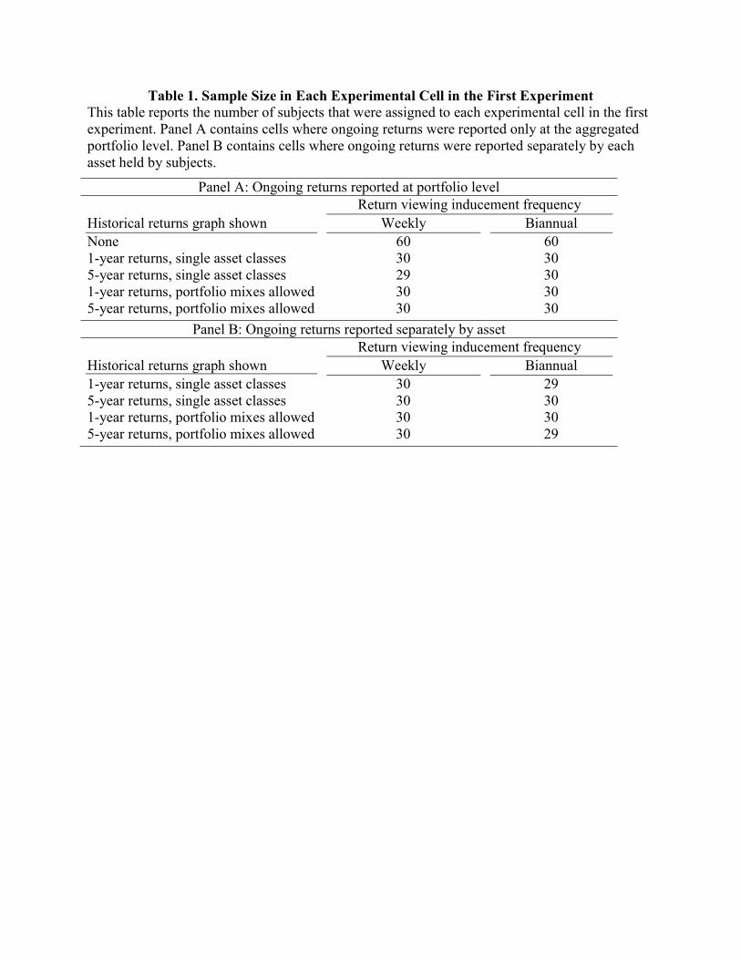
Table 1. Sample Size in Each Experimental Cell in the First Experiment This table reports the number of subjects that were assigned to each experimental cell in the first experiment. Panel A contains cells where ongoing returns were reported only at the aggregated portfolio level. Panel B contains cells where ongoing returns were reported separately by each asset held by subjects.

Panel A: Ongoing returns reported at portfolio level Return viewing inducement frequency Historical returns graph shown Weekly Biannual None 60 60 1-year returns, single asset classes 30 30 5-year returns, single asset classes 29 30 1-year returns, portfolio mixes allowed 30 30 5-year returns, portfolio mixes allowed 30 30

Panel B: Ongoing returns reported separately by asset Return viewing inducement frequency Historical returns graph shown Weekly Biannual 1-year returns, single asset classes 30 29 5-year returns, single asset classes 30 30 1-year returns, portfolio mixes allowed 30 30 5-year returns, portfolio mixes allowed 30 29

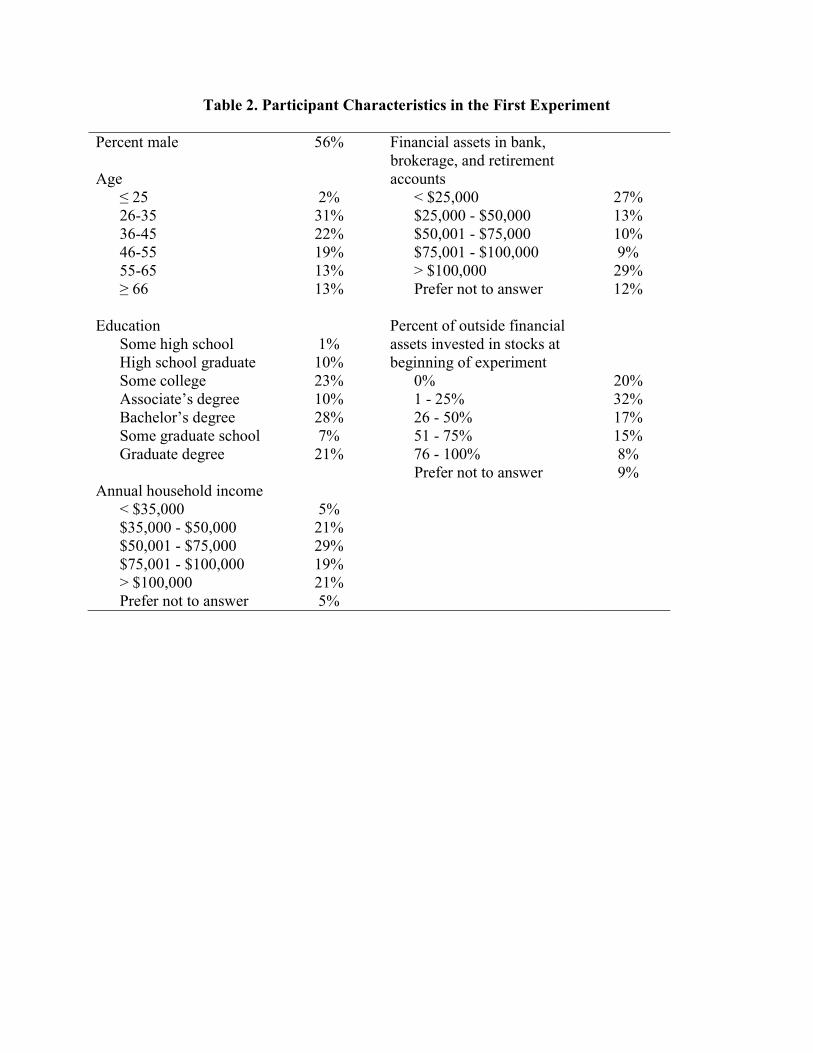
Table 2. Participant Characteristics in the First Experiment

Percent male 56% Financial assets in bank, brokerage, and retirement Age accounts

≤ 25 2% < $25,000 27% 26-35 31% $25,000 - $50,000 13% 36-45 22% $50,001 - $75,000 10% 46-55 19% $75,001 - $100,000 9% 55-65 13% > $100,000 29% ≥ 66 13% Prefer not to answer 12%

Education Percent of outside financial

Some high school 1% assets invested in stocks at High school graduate 10% beginning of experiment Some college 23% 0% 20% Associate’s degree 10% 1 - 25% 32% Bachelor’s degree 28% 26 - 50% 17% Some graduate school 7% 51 - 75% 15% Graduate degree 21% 76 - 100% 8%

Prefer not to answer 9% Annual household income

< $35,000 5% $35,000 - $50,000 21% $50,001 - $75,000 29% $75,001 - $100,000 19% > $100,000 21% Prefer not to answer 5%

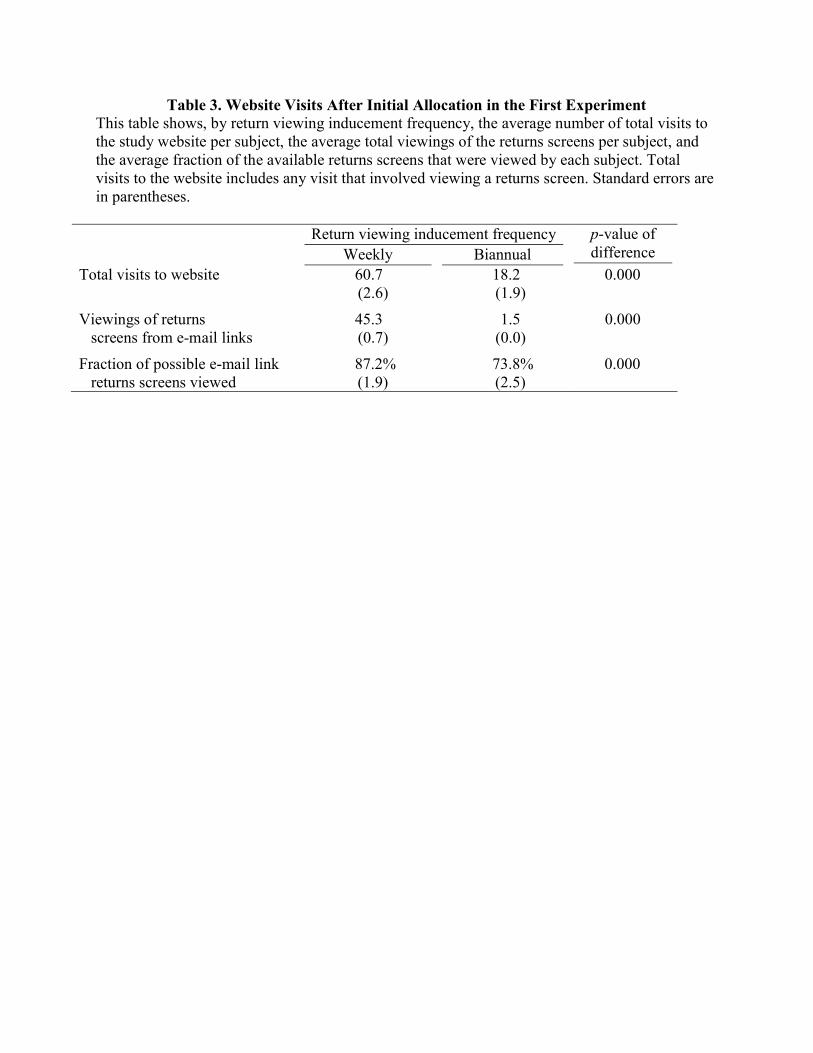
Table 3. Website Visits After Initial Allocation in the First Experiment This table shows, by return viewing inducement frequency, the average number of total visits to the study website per subject, the average total viewings of the returns screens per subject, and the average fraction of the available returns screens that were viewed by each subject. Total visits to the website includes any visit that involved viewing a returns screen. Standard errors are in parentheses.

Return viewing inducement frequency p-value of difference Weekly Biannual

Total visits to website 60.7 18.2 0.000 (2.6) (1.9)

Viewings of returns 45.3 1.5 0.000 screens from e-mail links (0.7) (0.0)

Fraction of possible e-mail link 87.2% 73.8% 0.000 returns screens viewed (1.9) (2.5)

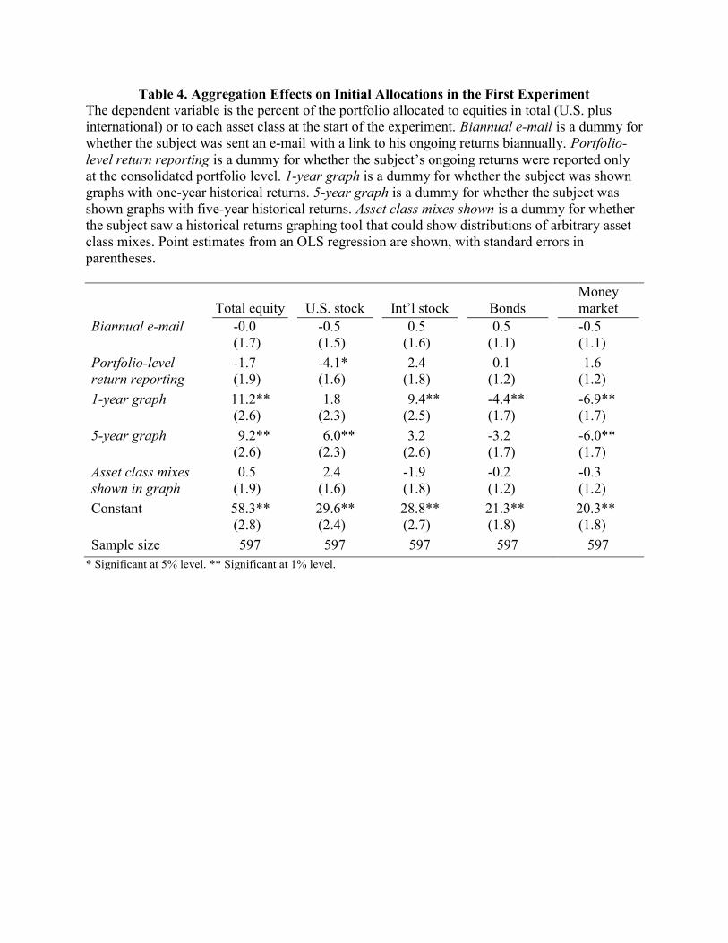
Table 4. Aggregation Effects on Initial Allocations in the First Experiment The dependent variable is the percent of the portfolio allocated to equities in total (U.S. plus international) or to each asset class at the start of the experiment. Biannual e-mail is a dummy for whether the subject was sent an e-mail with a link to his ongoing returns biannually. Portfolio-level return reporting is a dummy for whether the subject’s ongoing returns were reported only at the consolidated portfolio level. 1-year graph is a dummy for whether the subject was shown graphs with one-year historical returns. 5-year graph is a dummy for whether the subject was shown graphs with five-year historical returns. Asset class mixes shown is a dummy for whether the subject saw a historical returns graphing tool that could show distributions of arbitrary asset class mixes. Point estimates from an OLS regression are shown, with standard errors in parentheses.

Total equity U.S. stock Int’l stock Bonds Money market

Biannual e-mail -0.0 -0.5 0.5 0.5 -0.5 (1.7) (1.5) (1.6) (1.1) (1.1) Portfolio-level -1.7 -4.1* 2.4 0.1 1.6 return reporting (1.9) (1.6) (1.8) (1.2) (1.2) 1-year graph 11.2** 1.8 9.4** -4.4** -6.9** (2.6) (2.3) (2.5) (1.7) (1.7) 5-year graph 9.2** 6.0** 3.2 -3.2 -6.0** (2.6) (2.3) (2.6) (1.7) (1.7) Asset class mixes 0.5 2.4 -1.9 -0.2 -0.3 shown in graph (1.9) (1.6) (1.8) (1.2) (1.2) Constant 58.3** 29.6** 28.8** 21.3** 20.3** (2.8) (2.4) (2.7) (1.8) (1.8) Sample size 597 597 597 597 597

* Significant at 5% level. ** Significant at 1% level.

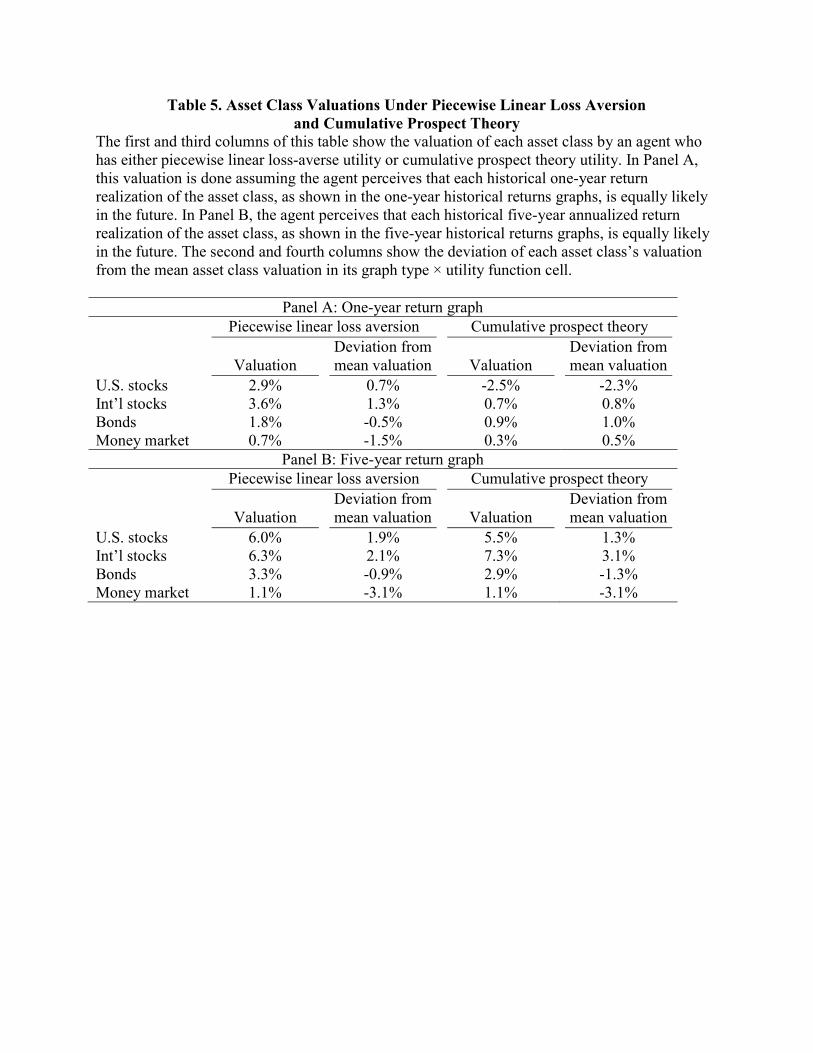
Table 5. Asset Class Valuations Under Piecewise Linear Loss Aversion and Cumulative Prospect Theory

The first and third columns of this table show the valuation of each asset class by an agent who has either piecewise linear loss-averse utility or cumulative prospect theory utility. In Panel A, this valuation is done assuming the agent perceives that each historical one-year return realization of the asset class, as shown in the one-year historical returns graphs, is equally likely in the future. In Panel B, the agent perceives that each historical five-year annualized return realization of the asset class, as shown in the five-year historical returns graphs, is equally likely in the future. The second and fourth columns show the deviation of each asset class’s valuation from the mean asset class valuation in its graph type × utility function cell.

Panel A: One-year return graph Piecewise linear loss aversion Cumulative prospect theory

Valuation Deviation from mean valuation Valuation

Deviation from mean valuation

U.S. stocks 2.9% 0.7% -2.5% -2.3% Int’l stocks 3.6% 1.3% 0.7% 0.8% Bonds 1.8% -0.5% 0.9% 1.0% Money market 0.7% -1.5% 0.3% 0.5%

Panel B: Five-year return graph Piecewise linear loss aversion Cumulative prospect theory

Valuation Deviation from mean valuation Valuation

Deviation from mean valuation

U.S. stocks 6.0% 1.9% 5.5% 1.3% Int’l stocks 6.3% 2.1% 7.3% 3.1% Bonds 3.3% -0.9% 2.9% -1.3% Money market 1.1% -3.1% 1.1% -3.1%

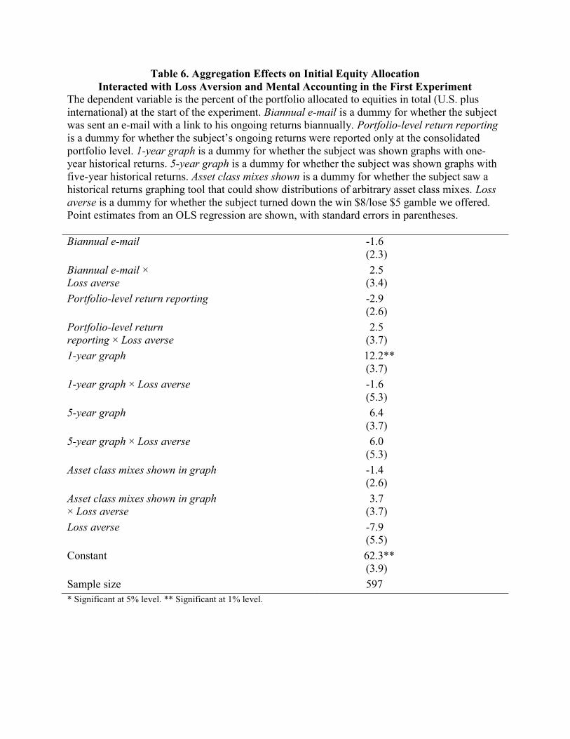
Table 6. Aggregation Effects on Initial Equity Allocation Interacted with Loss Aversion and Mental Accounting in the First Experiment

The dependent variable is the percent of the portfolio allocated to equities in total (U.S. plus international) at the start of the experiment. Biannual e-mail is a dummy for whether the subject was sent an e-mail with a link to his ongoing returns biannually. Portfolio-level return reporting is a dummy for whether the subject’s ongoing returns were reported only at the consolidated portfolio level. 1-year graph is a dummy for whether the subject was shown graphs with one-year historical returns. 5-year graph is a dummy for whether the subject was shown graphs with five-year historical returns. Asset class mixes shown is a dummy for whether the subject saw a historical returns graphing tool that could show distributions of arbitrary asset class mixes. Loss averse is a dummy for whether the subject turned down the win $8/lose $5 gamble we offered. Point estimates from an OLS regression are shown, with standard errors in parentheses. Biannual e-mail -1.6 (2.3) Biannual e-mail × 2.5 Loss averse (3.4) Portfolio-level return reporting -2.9 (2.6) Portfolio-level return 2.5 reporting × Loss averse (3.7) 1-year graph 12.2** (3.7) 1-year graph × Loss averse -1.6 (5.3) 5-year graph 6.4 (3.7) 5-year graph × Loss averse 6.0 (5.3) Asset class mixes shown in graph -1.4 (2.6) Asset class mixes shown in graph 3.7 × Loss averse (3.7) Loss averse -7.9 (5.5) Constant 62.3** (3.9) Sample size 597 * Significant at 5% level. ** Significant at 1% level.

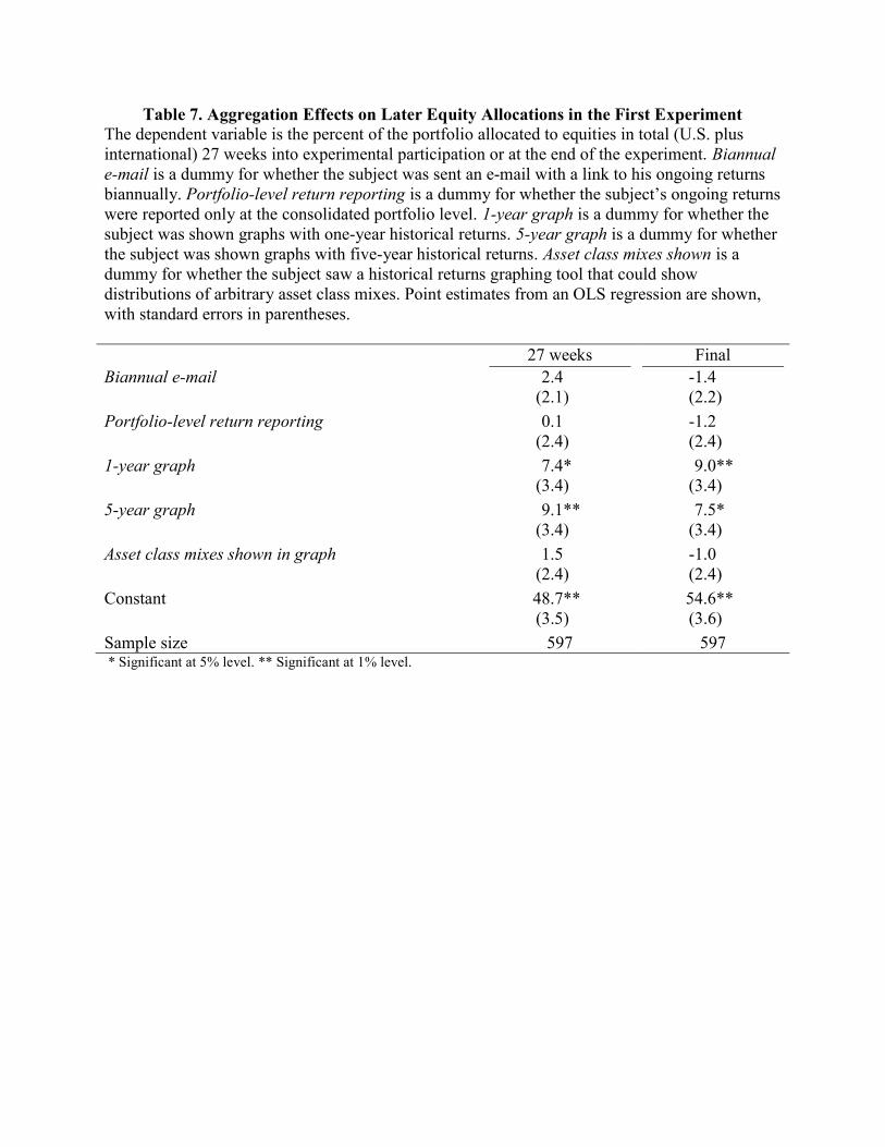
Table 7. Aggregation Effects on Later Equity Allocations in the First Experiment The dependent variable is the percent of the portfolio allocated to equities in total (U.S. plus international) 27 weeks into experimental participation or at the end of the experiment. Biannual e-mail is a dummy for whether the subject was sent an e-mail with a link to his ongoing returns biannually. Portfolio-level return reporting is a dummy for whether the subject’s ongoing returns were reported only at the consolidated portfolio level. 1-year graph is a dummy for whether the subject was shown graphs with one-year historical returns. 5-year graph is a dummy for whether the subject was shown graphs with five-year historical returns. Asset class mixes shown is a dummy for whether the subject saw a historical returns graphing tool that could show distributions of arbitrary asset class mixes. Point estimates from an OLS regression are shown, with standard errors in parentheses. 27 weeks Final Biannual e-mail 2.4 -1.4 (2.1) (2.2) Portfolio-level return reporting 0.1 -1.2 (2.4) (2.4) 1-year graph 7.4* 9.0** (3.4) (3.4) 5-year graph 9.1** 7.5* (3.4) (3.4) Asset class mixes shown in graph 1.5 -1.0 (2.4) (2.4) Constant 48.7** 54.6** (3.5) (3.6) Sample size 597 597 * Significant at 5% level. ** Significant at 1% level.

Table 8. Aggregation Effects on Initial Equity Allocation Interacted with Belief in Serially Uncorrelated Returns in the First Experiment

The dependent variable is the percent of the portfolio allocated to equities in total (U.S. plus international) at the start of the experiment. Biannual e-mail is a dummy for whether the subject was sent an e-mail with a link to his ongoing returns biannually. Portfolio-level return reporting is a dummy for whether the subject’s ongoing returns were reported only at the consolidated portfolio level. 1-year graph is a dummy for whether the subject was shown graphs with one-year historical returns. 5-year graph is a dummy for whether the subject was shown graphs with five-year historical returns. Asset class mixes shown is a dummy for whether the subject saw a historical returns graphing tool that could show distributions of arbitrary asset class mixes. Serially uncorrelated returns is a dummy for whether the subject believes that neither a 10% increase in the stock market last month nor a 10% decrease in the stock market last month should affect one’s forecast of the stock market’s return next month. Point estimates from an OLS regression are shown, with standard errors in parentheses. Biannual e-mail 1.2 (2.4) Biannual e-mail × -1.4 Serially uncorrelated returns (3.4) Portfolio-level return reporting -3.9 (2.7) Portfolio-level return 4.4 reporting × Serially uncorrelated returns (3.8) 1-year graph 7.4 (3.8) 1-year graph × Serially uncorrelated returns 7.0 (5.4) 5-year graph 8.5** (3.7) 5-year graph × Serially uncorrelated returns 1.8 (5.4) Asset class mixes shown in graph -1.4 (2.7) Asset class mixes shown in graph 4.3 × Serially uncorrelated returns (3.8) Serially uncorrelated returns -2.6 (5.6) Constant 59.2** (3.9) Sample size 570 * Significant at 5% level. ** Significant at 1% level.

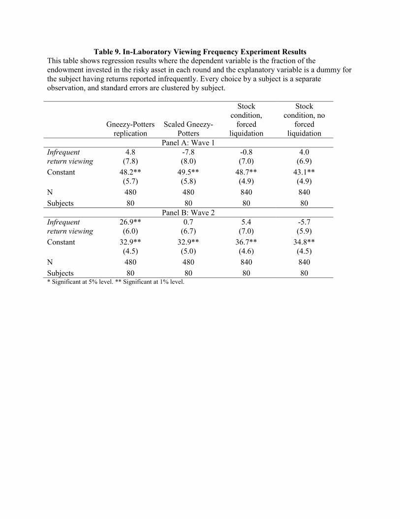
Table 9. In-Laboratory Viewing Frequency Experiment Results This table shows regression results where the dependent variable is the fraction of the endowment invested in the risky asset in each round and the explanatory variable is a dummy for the subject having returns reported infrequently. Every choice by a subject is a separate observation, and standard errors are clustered by subject.

Gneezy-Potters replication

Scaled Gneezy-Potters

Stock condition,

forced liquidation

Stock condition, no

forced liquidation

Panel A: Wave 1 Infrequent 4.8 -7.8 -0.8 4.0 return viewing (7.8) (8.0) (7.0) (6.9) Constant 48.2** 49.5** 48.7** 43.1** (5.7) (5.8) (4.9) (4.9) N 480 480 840 840 Subjects 80 80 80 80

Panel B: Wave 2 Infrequent 26.9** 0.7 5.4 -5.7 return viewing (6.0) (6.7) (7.0) (5.9) Constant 32.9** 32.9** 36.7** 34.8** (4.5) (5.0) (4.6) (4.5) N 480 480 840 840 Subjects 80 80 80 80 * Significant at 5% level. ** Significant at 1% level.

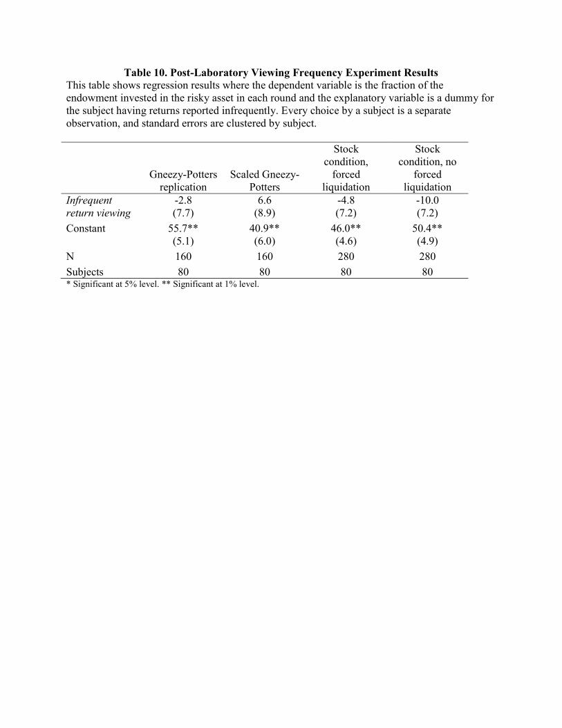
Table 10. Post-Laboratory Viewing Frequency Experiment Results This table shows regression results where the dependent variable is the fraction of the endowment invested in the risky asset in each round and the explanatory variable is a dummy for the subject having returns reported infrequently. Every choice by a subject is a separate observation, and standard errors are clustered by subject.

Gneezy-Potters replication

Scaled Gneezy-Potters

Stock condition,

forced liquidation

Stock condition, no

forced liquidation

Infrequent -2.8 6.6 -4.8 -10.0 return viewing (7.7) (8.9) (7.2) (7.2) Constant 55.7** 40.9** 46.0** 50.4** (5.1) (6.0) (4.6) (4.9) N 160 160 280 280 Subjects 80 80 80 80 * Significant at 5% level. ** Significant at 1% level.

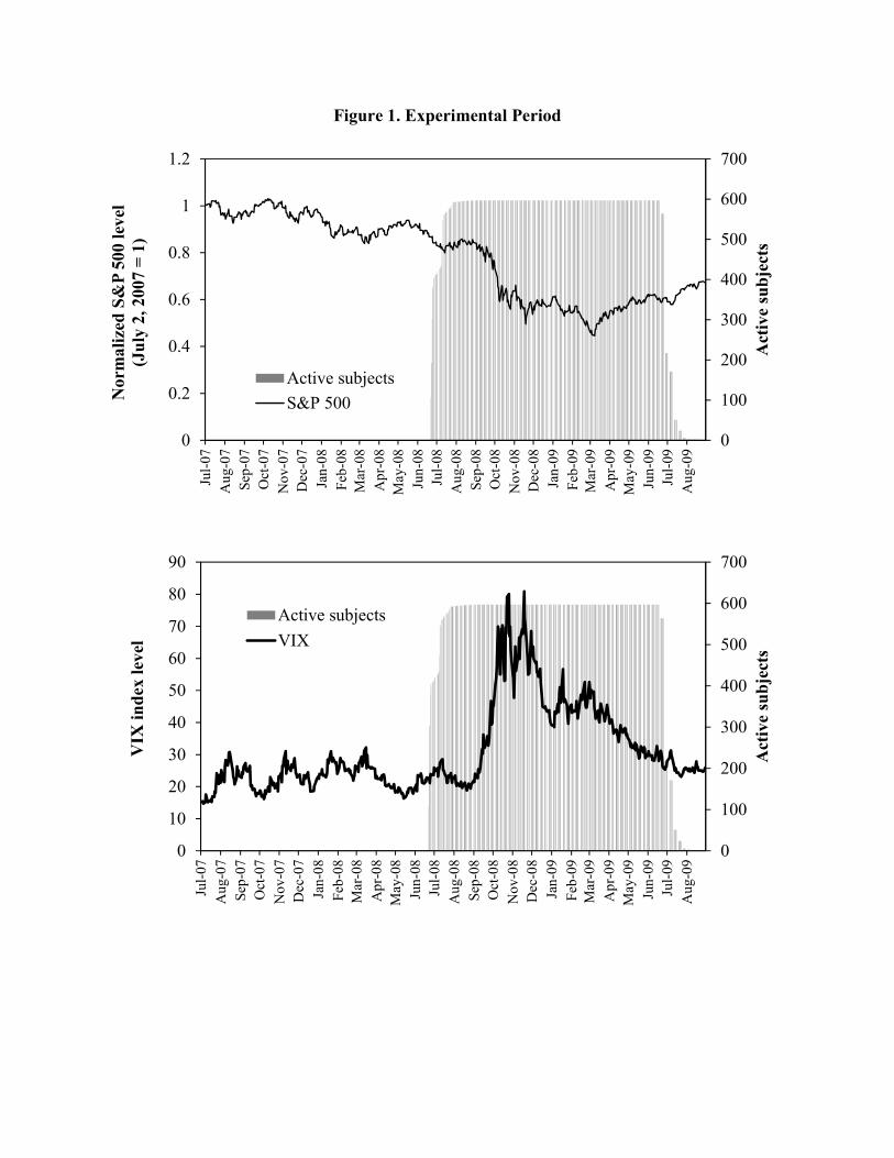
Figure 1. Experimental Period

0

100

200

300

400

500

600

700

0

0.2

0.4

0.6

0.8

1

1.2

Jul-0

7A

ug-0

7Se

p-07

Oct

-07

Nov

-07

Dec

-07

Jan-

08Fe

b-08

Mar

-08

Apr

-08

May

-08

Jun-

08Ju

l-08

Aug

-08

Sep-

08O

ct-0

8N

ov-0

8D

ec-0

8Ja

n-09

Feb-

09M

ar-0

9A

pr-0

9M

ay-0

9Ju

n-09

Jul-0

9A

ug-0

9

Act

ive

subj

ects

Nor

mal

ized

S&

P 50

0 le

vel

(Jul

y 2,

200

7 =

1)

Active subjectsS&P 500

0

100

200

300

400

500

600

700

0

10

20

30

40

50

60

70

80

90

Jul-0

7A

ug-0

7Se

p-07

Oct

-07

Nov

-07

Dec

-07

Jan-

08Fe

b-08

Mar

-08

Apr

-08

May

-08

Jun-

08Ju

l-08

Aug

-08

Sep-

08O

ct-0

8N

ov-0

8D

ec-0

8Ja

n-09

Feb-

09M

ar-0

9A

pr-0

9M

ay-0

9Ju

n-09

Jul-0

9A

ug-0

9

Act

ive

subj

ects

VIX

inde

x le

vel

Active subjectsVIX

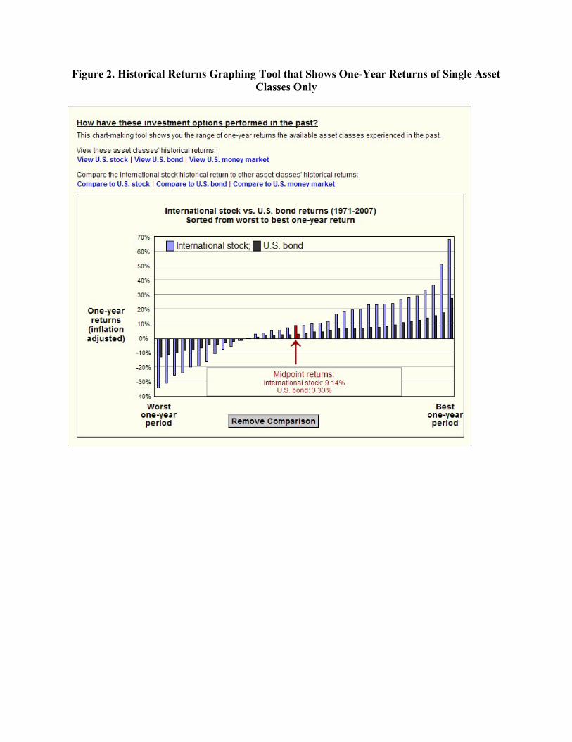
Figure 2. Historical Returns Graphing Tool that Shows One-Year Returns of Single Asset Classes Only

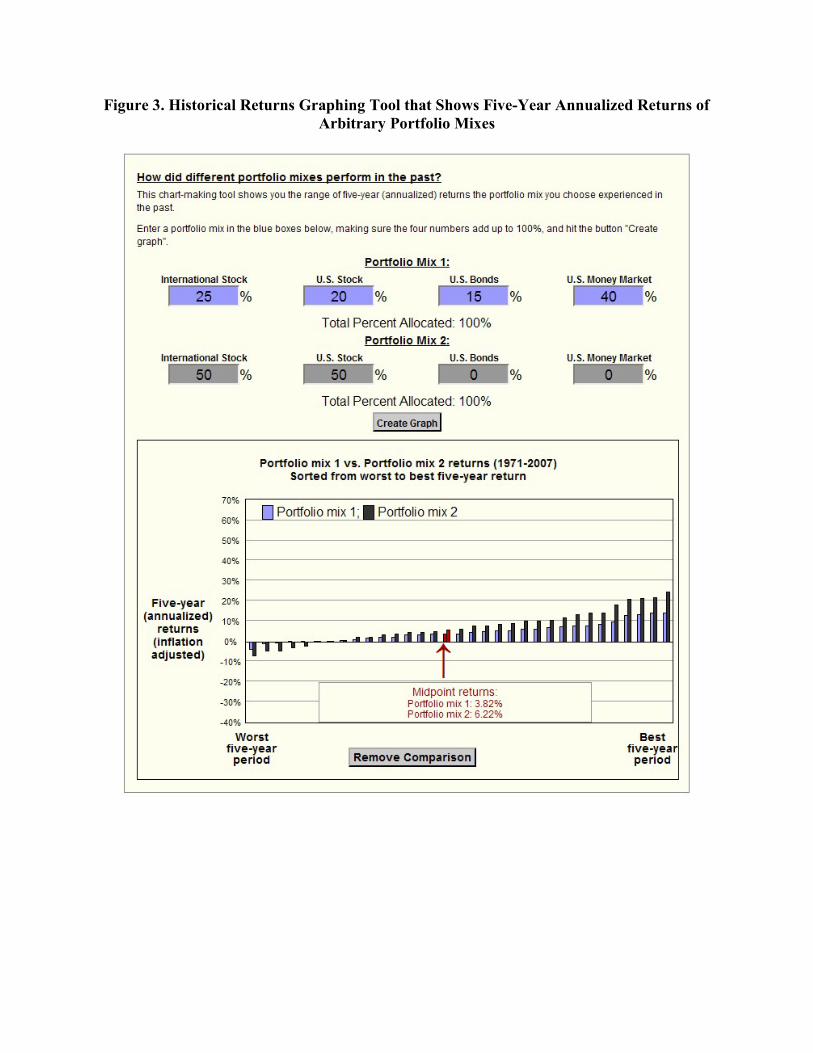
Figure 3. Historical Returns Graphing Tool that Shows Five-Year Annualized Returns of Arbitrary Portfolio Mixes

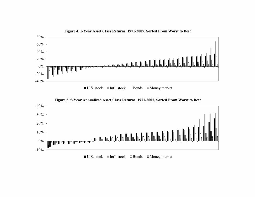
Figure 4. 1-Year Asset Class Returns, 1971-2007, Sorted From Worst to Best

Figure 5. 5-Year Annualized Asset Class Returns, 1971-2007, Sorted From Worst to Best

-40%

-20%

0%

20%

40%

60%

80%

U.S. stock Int’l stock Bonds Money market

-10%

0%

10%

20%

30%

40%

U.S. stock Int’l stock Bonds Money market

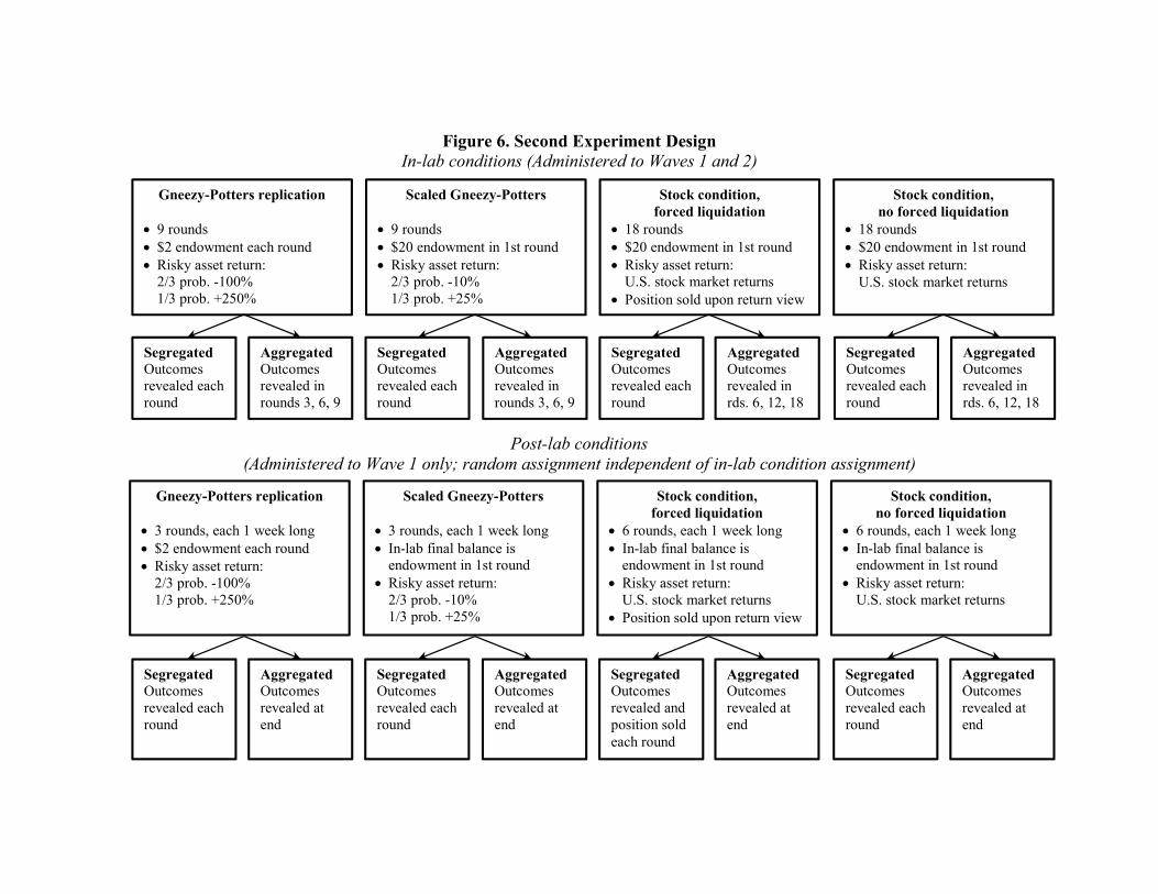
Figure 6. Second Experiment Design In-lab conditions (Administered to Waves 1 and 2)

Post-lab conditions (Administered to Wave 1 only; random assignment independent of in-lab condition assignment)

Gneezy-Potters replication

x 9 rounds x $2 endowment each round x Risky asset return:

2/3 prob. -100% 1/3 prob. +250%

Scaled Gneezy-Potters

x 9 rounds x $20 endowment in 1st round x Risky asset return:

2/3 prob. -10% 1/3 prob. +25%

Stock condition, forced liquidation

x 18 rounds x $20 endowment in 1st round x Risky asset return:

U.S. stock market returns x Position sold upon return view

Stock condition, no forced liquidation

x 18 rounds x $20 endowment in 1st round x Risky asset return:

U.S. stock market returns

Segregated Outcomes revealed each round

Aggregated Outcomes revealed in rounds 3, 6, 9

Segregated Outcomes revealed each round

Aggregated Outcomes revealed in rounds 3, 6, 9

Segregated Outcomes revealed each round

Aggregated Outcomes revealed in rds. 6, 12, 18

Segregated Outcomes revealed each round

Aggregated Outcomes revealed in rds. 6, 12, 18

Gneezy-Potters replication

x 3 rounds, each 1 week long x $2 endowment each round x Risky asset return:

2/3 prob. -100% 1/3 prob. +250%

Scaled Gneezy-Potters

x 3 rounds, each 1 week long x In-lab final balance is

endowment in 1st round x Risky asset return:

2/3 prob. -10% 1/3 prob. +25%

Stock condition, forced liquidation

x 6 rounds, each 1 week long x In-lab final balance is

endowment in 1st round x Risky asset return:

U.S. stock market returns x Position sold upon return view

Stock condition, no forced liquidation

x 6 rounds, each 1 week long x In-lab final balance is

endowment in 1st round x Risky asset return:

U.S. stock market returns

Segregated Outcomes revealed each round

Aggregated Outcomes revealed at end

Segregated Outcomes revealed each round

Aggregated Outcomes revealed at end

Segregated Outcomes revealed and position sold each round

Aggregated Outcomes revealed at end

Segregated Outcomes revealed each round

Aggregated Outcomes revealed at end