does climate aid affect emissions? evidence from a … · does climate aid affect emissions?...

Does Climate Aid Affect Emissions?

Evidence from a Global Dataset1

Sambit Bhattacharyya, Maurizio Intartaglia and Andy Mckay2

4 May, 2016

Abstract: We perform an empirical audit of the effectiveness of climate aid in tackling CO2

and SO2 emissions. Using a global panel dataset covering up to 131 countries over the period

1961 to 2011 and estimating a parsimonious model using the Anderson and Hsiao estimator

we do not find any evidence of a systematic effect of energy related aid on emissions. We

also find that the non-effect is not conditional on institutional quality or level of income.

Countries located in Europe and Central Asia does better than others in utilising climate aid

to reduce CO2 emissions. Our results are robust after controlling for the Environmental

Kuznets Curve, country fixed effects, country specific trends, and time varying common

shocks.

JEL classification: D72, O11

Key words: Climate Aid; Emissions; Energy

1We gratefully acknowledge financial support from the European Commission funded Seventh Framework

Programme (FP7) project entitled “Knowledge Based Climate Mitigation Systems for a Low Carbon Economy(COMPLEX)” [Grant Number: 308601]. We also acknowledge comments by and discussions with SaeedMoghaer, Elena Rovenskaya, Nick Winder, and Richard Tol. All viewpoints and any remaining errors are ourown and do not represent the views of the European Commission.2

Bhattacharyya: Department of Economics, University of Sussex, email: [email protected]: Department of Economics, University of Sussex, email: [email protected]; Mckay:Department of Economics, University of Sussex, email: [email protected].

#+164+!,24!6-+!&67*8!2,!",4.)(1!$)2120.+5

5GQCSUNGOU!PH!6EPOPNKET!"!@OKWGSTKUZ!PH!<YHPSF!"!9COPS!>PCF!3VKMFKOI!"!<YHPSF!<B)!+@=

[1!$,,!"(#)0.-!*/)(0,!"!M1!$,,!"(#)0.-!*0),,/!"!L1!ETCG&GORVKSKGT2GEPOPNKET&PY&CE&VL!"!^1!XXX&ETCG&PY&CE&VL

2

1 Introduction

Modern industrial society runs on fossil fuel. Burning fossil fuel releases thermal energy

which is then transformed into electricity. Electricity is a key input in the production of goods

and services destined for mass consumption. Consumers derive satisfaction from the

consumption of these mass produced goods. In modern society, sustained improvement in the

average level of consumption is a key indicator of material wellbeing and improved living

standards. The use of fossil fuel not only generates thermal energy but it also releases

greenhouse gases (carbon dioxide, sulphur dioxide, methane and others) into the atmosphere

causing global warming and climate change. Until recently the environmental consequences

of industrialisation were largely ignored. The global threat of a catastrophic climate change

has helped raise awareness and brought countries together in favour of a coordinated policy

response.

In a globalised world of free trade and migration (to a lesser extent), global

governance of climate change mitigation is challenging. It is relatively inexpensive for

industrial production to cross borders and move to cheaper locations. Indeed, starting from

the 1980s the world has noticed a significant dislocation of industries from the industrialised

nations to the emerging markets significantly increasing the latter’s share of greenhouse gas

emissions. Coupled with the global challenge of reducing greenhouse gas emissions the

abovementioned migration of polluting industries brings in a key question of distributive

justice in a Rawlsian sense3. To what extent the emerging market economies should be

allowed to emit so that the twin objectives of sustainable development and reducing global

greenhouse gas emissions could be achieved? Indeed these twin objectives are enshrined in

many of the official documents on climate change commissioned and authored by multilateral

3 Note that Rawls (1971) explicitly refrained from applying his principles of justice beyond theconfines of a territorial state. Relevance of Rawlsian principles to global governance were discussed in laterinterpretations elsewhere (see Pogge, 1989).

3

institutions. For example, the Clean Development Mechanism (CDM)4 defined in the Kyoto

Protocol also emphasises the importance of these twin objectives (IPCC, 2007). In particular,

the CDM aims to: (1) assist developing countries in achieving sustainable development while

preventing catastrophic climate change, and (2) help industrialised countries reach their

greenhouse gas emissions target.

At the operational level, states around the world have aimed to address these

challenges by making use of both bilateral and multilateral institutional mechanisms. In

particular, countries have used the mechanism of international transfers especially in the field

of energy to achieve the twin objectives of emissions reduction and sustainable development.

Policymakers have been using these policy tools for at least three decades now yet the effects

are not very well known. To the best of our knowledge, there is hardly any systematic

quantitative research on the effect of environmental aid on emissions in the aid recipient

countries. In this paper, we seek to explore this very question: Do we notice a perceptible

difference in the level of emissions in the aid recipient countries as a result of energy related

aid going back to the 1960s?

A cursory look at the global aggregates reveals that both foreign aid commitment and

disbursement for the energy sector (especially electricity generation) have exploded over the

last decade. For example, per capita aid disbursement for power generation over the 2000s

have grown by 4 percent on average every year whereas the annualised growth rate of aid

commitment in power generation for the same period is approximately 5 percent. Carbon

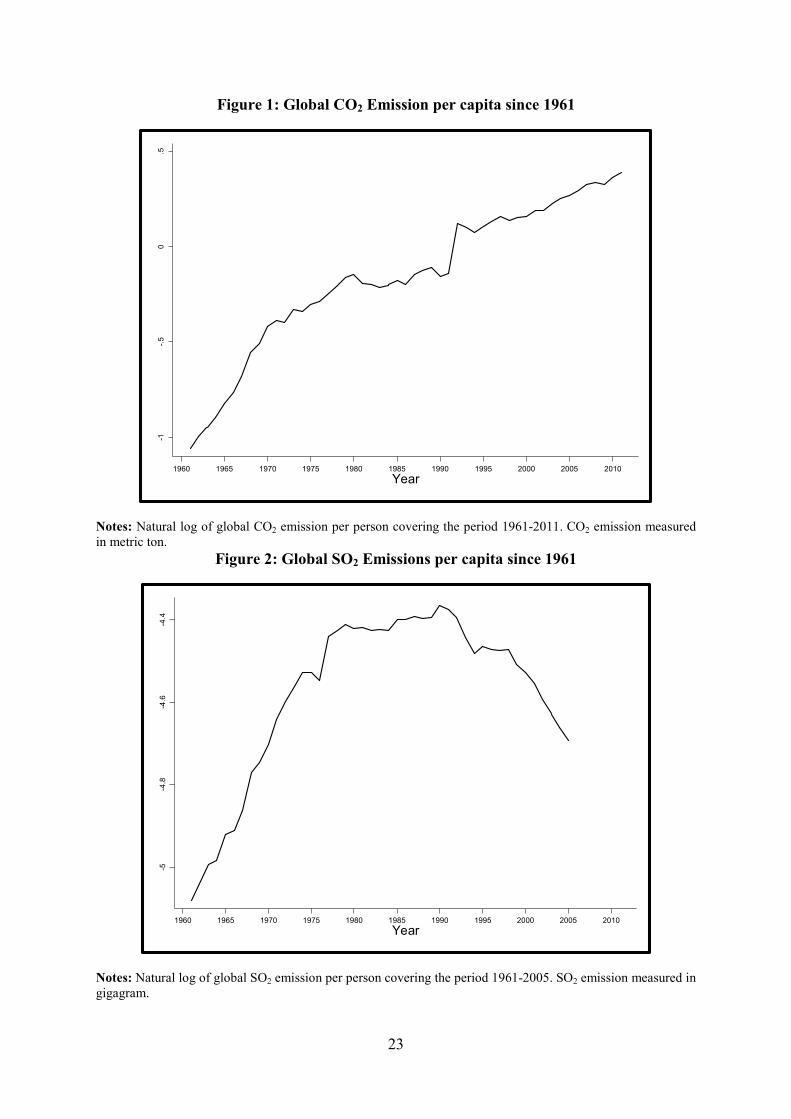
dioxide (CO2) emissions however have increased at an annualised rate of 2.5 percent over the

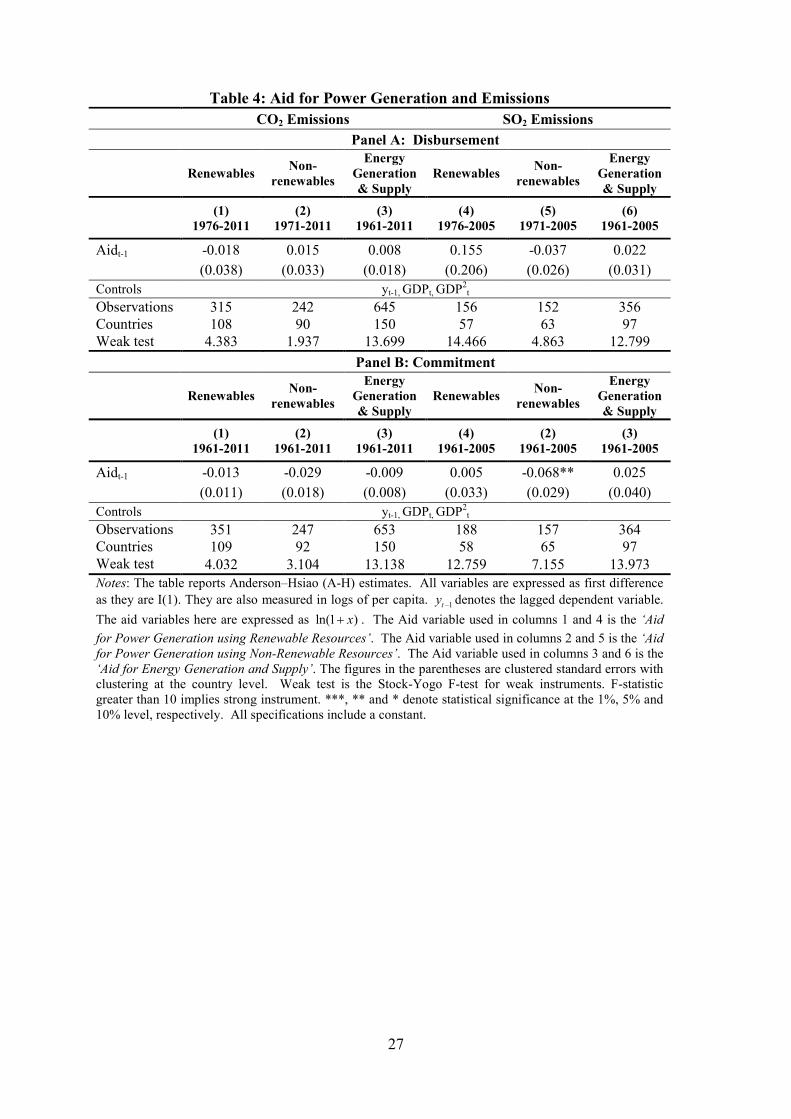
same period. Emissions of sulphur dioxide (SO2) have declined since the mid-1990s largely

due to the introduction and subsequent adoption of unleaded fuels for transport. Figures 1 – 4

presents this data.

4 The CDM is a mechanism intended to produce emission reduction units through certified projectswhich then could be traded in emissions trading schemes (ETS).

4

Even though there has been some degree of co-movement between emissions and

environmental aid it is problematic to interpret this association as causal. What we plot are

global trends which ignore variations within and across countries. A third latent factor could

also be responsible for the co-movement which hardly makes this perceived association

causal. Furthermore, there is no obvious theoretical prior when it comes to the effect of

environmental aid on emissions. On the one hand policymakers in donor countries would

expect results in terms of reduced emissions through better targeting of the energy

infrastructure in the recipient countries. On the other hand environmental aid could very well

be off target and is spent on projects that have little discernible impact on emissions.

Therefore, the lack of a strong prior either way makes this policy design a prime candidate

for empirical audit. A more detailed and systematic modelling is necessary to understand the

co-movement in the raw time series data.

In this paper we aim to systematically explore the effect of energy related aid on CO2

and SO2 emissions. In particular, we analyse the effect of an energy related aid shock on

emissions using a panel data model. We exploit a global panel dataset covering up to 131

countries over the period 1961 to 2011. Note that our aid data is sourced from AidData.org.

This dataset is an improvement over the Creditor Reporting System (CRS) maintained by the

OECD’s Development Assistance Committee (DAC) and offers far wider country coverage.

Furthermore, our dataset also allows us to distinguish between renewable and non-renewable

sources of power generation, and energy supply infrastructure. We estimate a parsimonious

model using fixed effects, Arellano and Bond, and Anderson and Hsiao estimators and do not

find any evidence of a systematic effect of energy related aid on emissions. Some would

argue that the effect of aid is perhaps conditional on country specific fundamentals such as

nature of policy or quality of institutions. We are unable to distinguish the average effect

from zero even after interacting the aid variable with the rule of law index, corruption, degree

5

of democracy, private property rights, government effectiveness, and openness to trade.

The zero effect could be driven by potential heterogeneity across very low income

and relatively advanced economies. It is entirely plausible that relatively advanced economies

are far more efficient in adopting greener technologies for power generation whereas the very

low income economies are rather slack. If this is indeed the case then one would expect to see

opposing effects across the two samples. To our surprise we observe no such evidence of

non-linearity in the relationship and the average effect stays zero.

We also test any potential heterogeneity across continents by dividing the sample into

Asia, Europe and Central Asia (ECA), Latin America and the Caribbean (LAC), and Middle

East and North Africa (MENA). With the exception of ECA the average effect remains zero

across all other continents. We notice some evidence of emission reduction as a result of

environmental aid in ECA. Our results are robust to the inclusion of country fixed effects,

country specific trends, time varying common shocks, GDP per capita, and GDP per capita

squared as controls. The exclusion of outliers and the inclusion of additional covariates such

as trade openness, urbanisation, human capital, investments, population density, and per

capita energy use do not alter our fundamental result of zero average effect.

Empirically identifying the causal effect of environmental aid on emissions is

challenging because potential biases from simultaneous and reverse causation. This challenge

is not specific to the macro environmental economics literature but in fact part of a broader

challenge associated with the aid and development literature. We follow the empirical

methodology of Clemens et al. (2012) to tackle identification challenges. Clemens et al.

(2012) argue that it may take time for most aid disbursement to have an impact on other

macroeconomic variables as they are generally lumpy and work through multiple channels.

Therefore, they show that transparent methods of lagging and differencing the data are

superior to using poor quality instrumental variables which tends to magnify the problem of

6

reverse causation. Following Clemens et al. (2012) we use five year averages as observations

and use lags in the model. The model is estimated using the Anderson and Hsiao method

along with fixed effects and Arellano and Bond dynamic panel data estimation methods.

Clemens et al. (2012) present Anderson and Hsiao estimates as their preferred results.

The paper makes the following contributions. First, it performs a much needed

econometric audit of the policy of environmental aid. Climate change is a major challenge of

our generation and it is extremely important that some of the existing macro policies are

thoroughly scrutinised using scientific means. To our surprise, we did not find any other

study asking the obvious question: what impact energy related aid has on emissions? Second,

by bringing this scientific result to the academy and the policymakers our paper opens the

way for much needed future scientific scrutiny of policies in this arena.

Our paper is related to a large literature on the determinants of emissions. This

literature could be divided into two strands: (1) a literature based on the Stochastic Impacts

by Regressions on Population, Affluence and Technology (SIRPAT) methodology and (2) a

literature based on the Environmental Kuznets Curve (EKC). Examples of the former are

Narayan and Narayan (2010), Menz and Kühling (2011), and Menz and Welsch (2012).

Narayan and Narayan (2010) focus on the effect of affluence by using economic growth as

the key explanatory variable whereas Cole and Nemayer (2004), Menz and Kühling (2011)

and Menz and Welsch (2012) focus on population size and population aging. Numerous other

studies seek to verify the EKC. The EKC model predicts an inverted U shaped relationship

between income and emissions. In other words, environmental pollution is increasing in

income up to a certain threshold beyond which environmental pollution is in fact declining in

the level of income. Torras and Boyce (1998), Auci and Becchetti (2006), and York et al.

(2003) are good examples of empirical studies of EKC. Dinda (2004) presents a review of the

EKC literature.

7

In addition to the SIRPAT and EKC based studies, a large literature examines

additional determinants of pollution. This literature finds that trade openness (Grossman and

Krueger, 1993), quality of political institutions (Scruggs, 1998; Farzin and Bond, 2006; and

Bernauer and Koubi, 2009), and urbanisation (Zhu et al., 2012; and Sadorsky, 2014) affects

air quality.

Finally, our paper is also related to a voluminous empirical literature on aid and

development. Griffin and Enos (1970) launch this literature with bivariate regressions on aid

and growth followed by Weisskopf (1972) and Papanek (1972). More recently some of the

notable studies are Boone (1996), Burnside and Dollar (2000), Collier and Dollar (2002),

Easterly (2003), Rajan and Subramanian (2008), and Clemens et al. (2012). In spite of the

volume of time and energy that economists have dedicated to debate the empirical

relationship between aid and growth, the issue still remains inconclusive.

The remainder of the paper is structured as follows: Section 2 discusses the empirical

strategy and data. Section 3 presents evidence on the effects of environmental aid on

emissions. It also distinctly examines the effects of aid in renewables, non-renewables, and

energy supply infrastructure on emissions. Furthermore, this section thoroughly examines any

potential good policy, governance or income based heterogeneity in the data. Section 4

reports on a battery of robustness tests and section 5 concludes.

2 Empirical Strategy

We use a panel dataset covering up to 131 countries observed over the period 1961 to 2011.5

To estimate the direct effects of environmental aid on emissions, we use the following

dynamic model:

1=

it it it j i itit t iE E Aid t u# #

" " "" % " "X (1)

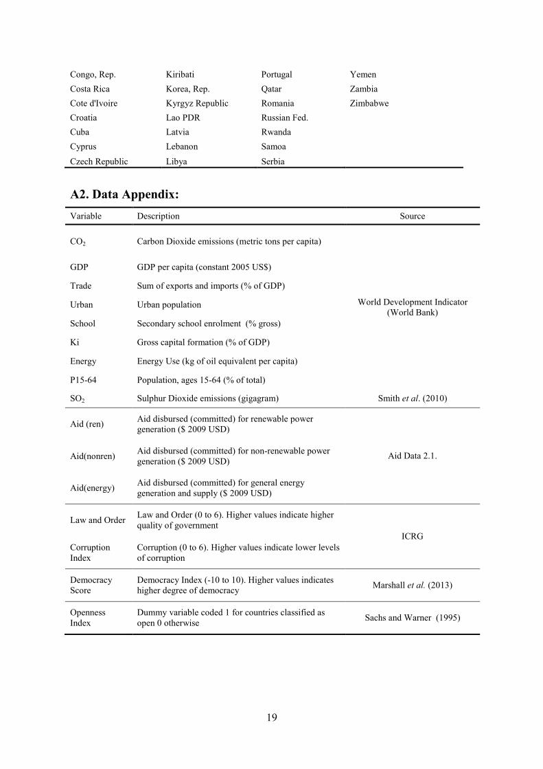
5 Due to data limitations, not all specifications cover 131 countries. In most specifications, the panel isunbalanced. The sample size is somewhat truncated for SO2 emissions and covers the time period 1961-2005.Missing data is the only reason behind excluding a country-year from the sample. Appendix A1 presents a list ofcountries included in the sample.

8

where itE represents emissions of CO2 and SO2 in country i at year t , i is the country

fixed effects, t is a year dummy variable controlling for time varying common shocks, it

are country specific time trends. Country specific trend captures potential country specific

time varying factors that might affect emissions. The variable it jAid # is an indicator of energy

related aid received by country i in the year t j# . We also control for additional covariates

including GDP per capita and GDP per capita squared. This is represented by the vector itX .

We estimate this model for contemporaneous effects and lags j thus {0,1}j , . All variables

in equation 1 are defined as per capita and expressed in natural logarithms with the exception

of the aid variable. The aid variable it jAid # is defined using the generic transformation

ln[1 ]x" to account for zero observations. This transformation eliminates excessive skewness

and kurtosis in the data. Furthermore, all observations used to estimate equation 1 are five

year averages. Thus, each country in the panel dataset includes a maximum of 11 vertical

(time series) data points with the 2010 data point being the average of the years 2010 and

2011.

Our main focus of enquiry is the effect of energy related aid it jAid # on emissions itE .

Therefore, our coefficient of interest is which represents the average marginal effect (or

elasticity) of environmental aid on emissions. A negative and statistically significant

coefficient would imply that environmental aid is effective in lowering the levels of CO2 and

SO2 emissions. Alternatively, a positive and statistically significant coefficient would imply

that a higher level of environmental aid is associated with adverse emissions outcome.

Finally, another potential possibility is that the average marginal effect cannot be

distinguished from zero which would imply that environmental transfers have very little

discernible effect on emissions in the aid recipient countries.

9

We include GDP per capita and GDP per capita squared to account for a potential

inverted U shaped relationship between the level of income and emissions commonly known

as Environmental Kuznets Curve (EKC). Shafik and Bandyopadhyay (1992), Panayotou,

(1993) and Grossman and Krueger (1993) were the first to detect such empirical relationship.

They provide evidence that while economic growth is detrimental to the environment at early

stages of development the relationship between environmental quality and economic growth

reverses beyond a threshold level of development.

Our key dependent variables ( itE ) are CO2 and SO2 emissions. The CO2 emissions

data is sourced from the World Development Indicators (WDI) database of the World Bank

and is measured in metric tons. This data is collected by the Carbon Dioxide Information

Analysis Centre of the Environmental Sciences Division, Oak Ridge National Laboratory of

the United States located in Tennessee. Atmospheric CO2 is a key contributor to climate

change and global temperature rise. Combustion of fossil fuels is the predominant source of

CO2 emissions.

The SO2 emissions data is sourced from Smith et al. (2010) who provide estimates of

global and country-level emissions over the period 1850 to 2005. The dataset has been

developed by using calibrated country-level inventories information compiled from a number

of sources. Note that Smith et al. (2010) reports SO2 emissions in gigagrams rather than

kilotons. To facilitate uniformity of measurement across the two emissions variables we

multiply SO2 emissions by 1000 to convert it into metric tons.

Unlike CO2, SO2 is a local pollutant. SO2 emissions mainly come from the

combustion of coal and petroleum. Emission levels of SO2 peaked in 1991 and since then it

experienced a steady decline. The decline in coal fired power stations in Europe and the

adoption of unleaded fuels for car may have contributed to this decline.

10

Environment quality is a multidimensional concept. Therefore there is some merit in

using a composite measure of environmental quality as opposed to emissions of individual

pollutants. One such measure is the Environmental Performance Index developed by

Emerson et al. (2010). This index is based on a large number of variables ranging from the

percentage of population with access to drinking water to CO2 emissions by the industrial

sector. However, poor data coverage is a major limitation of this dataset. Similarly, one could

also consider indices of other forms of environmental degradation. For example, one could

consider the measures of water quality, land degradation and deforestation. Again these

variables are restricted to a limited number of countries and time periods. In contrast, the CO2

and SO2 emissions data are available for a large number of countries and time periods. They

are also very widely used. It is worthwhile noting that we focus on emissions instead of

concentration of CO2 and SO2 because the former closely track economic activity rather than

the latter.

Rates of emission vary considerably across countries. For example, CO2 emission

ranges from 13.9 tons per capita in Chad over the period 1991 – 1995 to approximately 60

gigatons per capita in Qatar over the period 1996 – 2000. In contrast, SO2 emission ranges

from 0.2 tons per capita in Botswana over the period 1976 – 1980 to 403 tons per capita in

Zambia over the period 1961 – 1965.

Our key independent variable is energy related aid. This data is sourced from the

AidData.org, research release 2.1. This dataset is compiled by Tierney et al. (2011). The

Tierney et al. (2011) database distinguishes between development finance as loans from

governments or agencies from transfers. The AidData.org project is run by the Bingham

Young University, the College of William and Mary, and the Development Gateway. It

emerged out of two earlier projects on the Accessible Information on Development Activities

and Project-Level Aid. Both projects compiled project level aid data.

11

The bulk of the data in AidData.org comes from the Creditor Reporting System

(CRS), which collects annual data from 22 member countries dating back to 1973. In addition

to CRS, AidData.org also includes data from other official sources. For instance, it records

bilateral donations from non-OECD donors to non-DAC recipients as well as donations from

multilateral organisations. In line with CRS, AidData.org adopts a five digit classification

system of projects. The classification system identifies the sector, the activity code, and the

purpose of each project. A major advantage of the dataset is that it distinguishes between aid

commitment and aid disbursement. The 2.1 research release that we use covers a large

number of countries over the period 1947 to 2011.6

AidData.org records aid commitment and disbursement for a large variety of projects.

We limit our attention to aid for environmental projects. In particular, we focus on: (i) power

generation projects from renewable sources, (ii) power generation projects from non-

renewable sources and (iii) energy generation and supply projects. The energy generation and

supply projects include power generation from renewables and non-renewables, energy

policy and administrative management, energy transmission, energy education, and energy

research.7

A zero value for the aid variable would imply that the donors did not commit or

disburse any money. A quick scrutiny of the raw data reveals that Palau received the highest

amount of energy related international financial assistance over the period 1996 – 2000 (USD

554 in 2009 constant prices) closely followed by Iceland 1966-1970 (USD 502 in 2009

constant prices) and Bahrain 1976-1980 (USD 432 in 2009 constant prices).

Other variables used in the study are: GDP per capita, law and order index,

corruption, democracy scores, trade openness index, trade share, private property rights,

6 We only use data from 1960 because the CO2 emissions data starts at 1960.7 Note that power generation from renewables and non-renewables correspond to the purpose codes

23020 and 23030. The energy generation and supply corresponds to the following purpose codes: 23000, 23005,23010, 23020, 23030, 23040, 23050, 23061, 23062, 23063, 23064, 23065, 23066, 23067, 23067, 23068, 23069,23070, 23081 and 23082.

12

government effectiveness. Tables 1 reports summary statistics on key variables and Appendix

A2 presents detailed definition of variables.

There are econometric challenges associated with estimating equation 1. These

challenges are unobserved heterogeneity, non-stationarity of the variables, reverse causation,

simultaneity bias, and bias due to the dynamic nature of the model. We closely follow

Clemens et al. (2010) to tackle these challenges. We address the unobserved heterogeneity

challenge by demeaning the data and estimating the model using fixed effects. However, the

fixed effect estimator is unable to tackle the challenge of non-stationarity. In a time series

dataset variables could have similar trends yielding statistically significant correlation.

However, this correlation could simply be reflective of their co-movement and not a causal

relationship. Therefore, estimating econometric models with variables that have a significant

time dimension and are not stationary would lead to spurious inference of causality when

there is none. To address this challenge we check stationarity of the variables by using the

Fisher type Adjusted Dickey Fuller (ADF), Levin–Lin–Chu, and Harris–Tzavalis varieties of

unit root tests. The Levin–Lin–Chu and the Harris–Tzavalis tests account for bias emanating

from cross-sectional association. We find that the key variables are I(1) or difference

stationary and therefore we use first difference of variables in the regressions. These tests are

reported in table 2. Note that Clemens et al. (2012) also reports similar results in the context

of aid and growth.

The level of emissions might dictate environmental aid flows rather than causality

running in the opposite direction. We address reverse causation and simultaneity challenges

by using five year averages and lags. An alternative approach is to use the instrumental

variable (IV) method. However, Clemens et al. (2012) demonstrates that using lags is a much

cleaner and transparent way of dealing with reverse causation as opposed to searching for an

appropriate instrument. Furthermore, they also show that the paucity of strong and valid

13

instruments permeates the aid and growth literature.

Finally, using a lagged dependent variable as an independent variable in the model

invites additional challenges. In particular, the differenced lagged dependent variable

1itE #$ could be correlated with the differenced error term itu$ contaminating inference.

However, for serially uncorrelated errors itu$ would not be correlated with 2itE #$ opening the

possibility of using 2itE #$ as an instrument for 1itE #$ . This is precisely what the Anderson

and Hsiao (1981) estimator does which we adopt here.

3 Evidence

3.1 Climate Aid and Emissions: Baseline Results

Table 3 conducts an empirical audit of the effects of climate aid on emissions. The key

independent variable here is the aid for power generation using both renewable and non-

renewable resources. We first concentrate on the effect of aid disbursement in panel A. In

column 1 we estimate equation 1 using the fixed effect estimator. We find that 1 percentage

point increase in aid for power generation using either renewable or non-renewable resources

reduce per capita CO2 emissions by 0.03 percent. To put this into perspective, a 0.03 percent

decline in per capita CO2 emission is equivalent to Qatar’s emission over the period 1996 –

2000 declining from 60 gigatons per person to 59.8 gigatons per person. Even though the

coefficient on aid is significant, we cannot be confident that it is precisely estimated. The

estimate could very well be driven by omitted factors or reverse causation. In column 2, we

replace the contemporaneous aid variable by lagged aid. The average effect of lagged aid on

per capita CO2 emission becomes indistinguishable from zero. In column 3 we estimate the

model using the Anderson and Hsiao instrumental variable method and the null effect result

remains. Note that this is also the preferred method of Clemens et al. (2012).

Since we are estimating a dynamic model with a lagged dependent variable, therefore

there is merit in pursuing the Arellano and Bond estimation method. We do exactly that in

14

column 4 without much difference in outcome. The average effect of lagged aid on per capita

CO2 emission cannot be distinguished from zero.

In columns 5 – 8 we repeat these estimates to explain variation in another important

pollutant SO2. Irrespective of the estimator used, we are unable to distinguish the average

effect of aid disbursement for power generation using renewables and non-renewables from

zero. In panel B we verify whether the effect is any different with aid commitment as the key

independent variable as opposed to actual aid disbursement. It is plausible even though

unlikely that aid commitments might affect expectations and preferences of policymakers in

aid recipient countries incentivising them to implement emission reduction plans. We find

that aid commitments have very little discernible impact on per capita emissions.

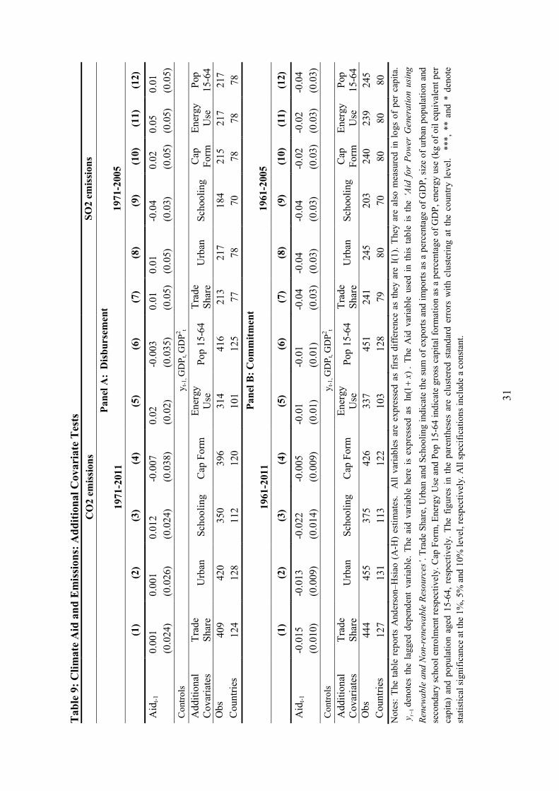
It is possible that by aggregating aid for power generation in renewable and non-

renewable sources we are weakening statistical power. Perhaps there is heterogeneity in the

data. At least in theory, increasing the share of power generation using renewable resources

could rapidly reduce emissions. In contrast upgrading existing non-renewable resource based

power plants or building new power plants may not have the desired emissions reducing

effect. Therefore we divide the aid data for power generation into renewables and non-

renewables in table 4 columns 1, 2, 4, and 5. The effect stays insignificantly different from

zero.

In columns 3 and 6 we explore any potential impact of aid in energy generation and

supply. Energy generation and supply is a broad measure of climate aid which includes

power generation, energy policy and administration, energy transmission infrastructure,

energy awareness education, and energy research. To our surprise we do not find any effect

of such aid on per capita emissions after controlling for country specific and global factors.

3.2 Climate Aid and Emissions: The Role of Institutions and Policy

15

The effectiveness of aid could be conditional on the country specific initial conditions.

Countries that have good policy and good institutions could be in a far better position to

respond to aid than others. Emissions respond better to aid in these locations because efficient

policy and institutions channel the funds effectively to the appropriate projects reducing

waste and administrative obstacles. If this is indeed the case then we would expect to see

non-linear effects of institutional quality on emissions.

We test the role of policy and institutions by introducing interaction terms in table 5.

In particular, we interact the aid for power generation variable with the rule of law index,

corruption, democracy scores, private property rights, government effectiveness, and Sachs

and Warner trade openness index. We do not find any evidence of non-linearity in the data.

The average effect of climate aid on CO2 and SO2 emissions is zero regardless of the quality

of institutions.

3.3 Climate Aid and Emissions: Is there a Rich and Poor Divide?

Upgrading to a new energy infrastructure or building a new power plant is not costless. On

the contrary these ventures are often expensive and require additional resources on top of the

aid money. Richer nations could afford these ventures and therefore they are far more

effective in upgrading their energy infrastructure or building new power plants. They could

also tap into a relatively skilled labour force to work on energy related projects. All this taken

together could contribute positively towards reducing per capita emissions.

If the hypothesis outlined above is indeed true then we would expect to see

heterogeneity in the data along income lines. However, in table 6 we do not find any evidence

that the level of income influences the effectiveness of climate aid.

3.3 Climate Aid and Emissions: The Role of Geography

Certain geographic locations could possess an advantage over others when it comes to

implementing emission reduction policies. Cleaning up the energy sector, upgrading to a new

16

energy infrastructure, and building new power plants require significant investments. It also

requires importation of capital goods and skills. Therefore, proximity to these inputs matter.

If a country is located in the same neighbourhood where green technology is advancing then

it is likely to be part of the same network. The countries are more likely to utilise their

climate aid money effectively.

We test this hypothesis in table 7 by estimating our canonical model separately for

Asia, Europe and Central Asia (ECA), Latin America and the Caribbean (LAC), and Middle

East and North Africa (MENA). We find that ECA countries are far more effective in

reducing their CO2 emissions using aid. Numerically, we find that 1 percentage point increase

in aid for power generation would reduce CO2 emissions by 0.31 percent. This amounts to

approximately 0.3 ton reduction in per capita emission in an average ECA country.

4 Robustness

The non-relationship between climate aid and emissions could be driven by outliers or

omitted variables. We check the robustness of our main result by controlling for outliers and

omitted covariates. In table 8 we estimate the model by eliminating potential outliers from the

sample. We do this systematically by identifying outliers using the formulas of DFITS,

Cooks Distance, and Welsch Distance. Dropping outliers from the sample do not alter our

main result.

In table 9 we introduce additional control variables. The environmental studies

literature have identified trade openness, urbanisation, school enrolment, investments, energy

use, and the fraction of population aged between 15 to 64 as important determinants of CO2

and SO2 emissions. We control for these variables and observe that the ineffectiveness of

climate aid on emissions remains.

5 Conclusions

Climate change and global temperature rise are significant challenges of our generation. The

17

recent climate change conference COP21 held in Paris in December 2015 calls for

greenhouse gas emissions to a level consistent with an average global temperature rise of 2

degrees (possibly 1.5 degrees) above pre-industrial average temperature. A significant

reduction in greenhouse gas emissions would be required in order to achieve this target.

Nations and multilateral organisations have used a plethora of policy tools to achieve

emissions reduction. One such policy is energy related international transfers. The idea is to

assist aid recipient countries to clean up existing energy infrastructure, build new greener

power plants, and switch from fossil fuel based energy mix to a renewables based energy

mix. Undoubtedly this is a worthy cause and donor countries have devoted significant amount

of resources to support this venture. Yet we know very little about the potential outcome of

this policy.

In this paper we perform an empirical audit of this policy by systematically exploring

the effect of energy related aid on CO2 and SO2 emissions. Using a global panel dataset

covering up to 131 countries over the period 1961 to 2011 and estimating a parsimonious

model using fixed effects, Arellano and Bond, and Anderson and Hsiao estimators we do not

find any evidence of a systematic effect of energy related aid on emissions. To our surprise,

we also find that the non-effect is not conditional on institutional quality or level of income.

Countries located in ECA do better than others in utilising climate aid to reduce CO2

emissions. Our results are robust to the inclusion of country fixed effects, country specific

trends, time varying common shocks, GDP per capita, and GDP per capita squared as

controls. The exclusion of outliers and the inclusion of additional covariates such as trade

openness, urbanisation, human capital, investments, population density, per capita energy

use, and the share of adult population do not alter our fundamental result of zero average

effect.

This result calls into question the merit of climate aid as a policy tool to achieve the

18

emission reduction objectives outlined in the Kyoto Protocol and beyond. It exposes that aid

of this nature has been fairly ineffective in the past. Therefore, policymakers would need to

be more circumspect while applying aid as a policy tool to address climate change. At the

very least our result calls for more scientific scrutiny of energy related aid.

Appendices

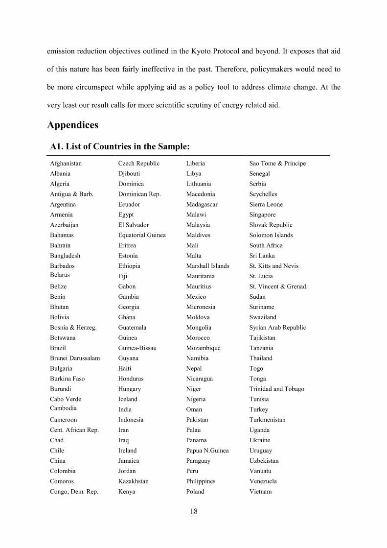
A1. List of Countries in the Sample:

Afghanistan Czech Republic Liberia Sao Tome & Principe

Albania Djibouti Libya Senegal

Algeria Dominica Lithuania Serbia

Antigua & Barb. Dominican Rep. Macedonia Seychelles

Argentina Ecuador Madagascar Sierra Leone

Armenia Egypt Malawi Singapore

Azerbaijan El Salvador Malaysia Slovak Republic

Bahamas Equatorial Guinea Maldives Solomon Islands

Bahrain Eritrea Mali South Africa

Bangladesh Estonia Malta Sri Lanka

Barbados Ethiopia Marshall Islands St. Kitts and Nevis

Belarus Fiji Mauritania St. Lucia

Belize Gabon Mauritius St. Vincent & Grenad.

Benin Gambia Mexico Sudan

Bhutan Georgia Micronesia Suriname

Bolivia Ghana Moldova Swaziland

Bosnia & Herzeg. Guatemala Mongolia Syrian Arab Republic

Botswana Guinea Morocco Tajikistan

Brazil Guinea-Bissau Mozambique Tanzania

Brunei Darussalam Guyana Namibia Thailand

Bulgaria Haiti Nepal Togo

Burkina Faso Honduras Nicaragua Tonga

Burundi Hungary Niger Trinidad and Tobago

Cabo Verde Iceland Nigeria Tunisia

Cambodia India Oman Turkey

Cameroon Indonesia Pakistan Turkmenistan

Cent. African Rep. Iran Palau Uganda

Chad Iraq Panama Ukraine

Chile Ireland Papua N.Guinea Uruguay

China Jamaica Paraguay Uzbekistan

Colombia Jordan Peru Vanuatu

Comoros Kazakhstan Philippines Venezuela

Congo, Dem. Rep. Kenya Poland Vietnam

19

Congo, Rep. Kiribati Portugal Yemen

Costa Rica Korea, Rep. Qatar Zambia

Cote d'Ivoire Kyrgyz Republic Romania Zimbabwe

Croatia Lao PDR Russian Fed.

Cuba Latvia Rwanda

Cyprus Lebanon Samoa

Czech Republic Libya Serbia

A2. Data Appendix:

Variable Description Source

CO2 Carbon Dioxide emissions (metric tons per capita)

World Development Indicator(World Bank)

GDP GDP per capita (constant 2005 US$)

Trade Sum of exports and imports (% of GDP)

Urban Urban population

School Secondary school enrolment (% gross)

Ki Gross capital formation (% of GDP)

Energy Energy Use (kg of oil equivalent per capita)

P15-64 Population, ages 15-64 (% of total)

SO2 Sulphur Dioxide emissions (gigagram) Smith et al. (2010)

Aid (ren)Aid disbursed (committed) for renewable powergeneration ($ 2009 USD)

Aid Data 2.1.Aid(nonren)Aid disbursed (committed) for non-renewable powergeneration ($ 2009 USD)

Aid(energy)Aid disbursed (committed) for general energygeneration and supply ($ 2009 USD)

Law and OrderLaw and Order (0 to 6). Higher values indicate higherquality of government

ICRGCorruptionIndex

Corruption (0 to 6). Higher values indicate lower levelsof corruption

DemocracyScore

Democracy Index (-10 to 10). Higher values indicateshigher degree of democracy

Marshall et al. (2013)

OpennessIndex

Dummy variable coded 1 for countries classified asopen 0 otherwise

Sachs and Warner (1995)

20

References

Anderson, T. W. and C. Hsiao (1982). Formulation and Estimation of Dynamic Models

Using Panel Data. Journal of econometrics, 18(1): 47-82.

Auci, S., and L. Becchetti (2006). The Instability of the Adjusted and Unadjusted

Environmental Kuznets Curves. Ecological Economics, 60(1): 282-298.

Bernauer, T., and V. Koubi (2009). Effects of Political Institutions on Air Quality. Ecological

Economics, 68(5): 1355-1365.

Boone, P. (1996). Politics and the Effectiveness of Foreign Aid. European Economic Review,

40(2): 289-329.

Burnside, C. and D. Dollar (2000). Aid, Policies, and Growth. American Economic Review,

90(4): 847–68.

Clemens, M. A., S. Radelet, R. R. Bhavnani and S. Bazzi (2012). Counting Chickens When

They Hatch: Timing and the Effects of Aid on Growth. The Economic Journal, 122(561):

590-617.

Collier, P. and D. Dollar (2002). Aid Allocation and Poverty Reduction. European Economic

Review, 46(8): 1475-1500.

Dinda, S. (2004). Environmental Kuznets Curve Hypothesis: A Survey. Ecological

Economics, 49(4): 431-455.

Easterly, W. (2003). Can Foreign Aid Buy Growth? Journal of Economic Perspectives,

17(3): 23-48.

Emerson, J., D. C. Esty, C. Kim, T. Srebotnjak, M. A. Levy, V. Mara, A. Sherbinin and M.

Jaiteh (2010). Environmental Performance Index. New Haven: Yale Center for

Environmental Law and Policy.

Farzin, Y. H., and C. A. Bond (2006). Democracy and Environmental Quality. Journal of

Development Economics, 81(1): 213-235.

21

Griffin, K. B., and J. L. Enos (1970). Foreign Assistance: Objectives and Consequences.

Economic Development and Cultural Change, 18(3): 313-327.

Grossman, G. M., and A. B. Krueger (1993). Environmental Impacts of the North American

Free Trade Agreement. In P. Garber, eds.: The U.S. –Mexico Free Trade Agreement. MIT

Press, Cambridge, pp. 13–56.

IPCC. (2007). Climate Change 2007: Report of the Intergovernmental Panel on Climate

Change. Cambridge University Press, Cambridge: UK and New York.

Menz, T., and J. Kühling (2011). Population Aging and Environmental Quality in OECD

Countries: Evidence from Sulfur Dioxide Emissions Data. Population and Environment,

33(1): 1-25.

Menz, T. and H. Welsch (2012). Population Aging and Carbon Emissions in OECD

Countries: Accounting for Life-Cycle and Cohort Effects. Energy Economics, 34(3): 842-

849.

Narayan, P. K., and S. Narayan (2010). Carbon Dioxide Emissions and Economic Growth:

Panel Data Evidence from Developing Countries. Energy Policy, 38(1): 661-666.

Panayotou, T. (1993). Empirical Tests and Policy Analysis of Environmental Degradation at

Different Stages of Economic Development. ILO, Technology and Employment Programme,

Geneva.

Papanek, G. (1972). The Effect of Aid and Other Resource Transfers on Savings and Growth

in Less Developed Countries. Economic Journal, 82(327): 934-950.

Pogge, T. (1989). Realizing Rawls. Cornell University Press, Ithaca: New York.

Rajan, R., and A. Subramanian (2008). Aid and Growth: What Does the Cross-Country

Evidence Really Show? The Review of Economics and Statistics, 90(4): 643-665.

Rawls, J. (1971). A Theory of Justice. Harvard University Press, Cambridge: MA.

22

Sadorsky, P. (2014). The Effect of Urbanization on CO2 Emissions in Emerging Economies.

Energy Economics, 41: 147-153.

Scruggs, L. A. (1998). Political and Economic Inequality and the Environment. Ecological

Economics, 26(3): 259-275.

Shafik, N., and S. Bandyopadhyay (1992). Economic Growth and Environmental Quality:

Time Series and Cross country Evidence. Background Paper for the World Development

Report 1992, The World Bank, Washington, DC.

Smith, S., J. Van Aardenne, Z. Klimont, R. J. Andres, A. Volke, and S. D. Arias (2010).

Anthropogenic Sulfur Dioxide Emissions: 1850–2005. Atmospheric Chemistry and Physics

Discussions, 10 (6): 16111-16151.

Tierney, M., D. L. Nielson, D. G. Hawkins, J. T. Roberts, M. G. Findley, R. M. Powers, B.

Parks, S. E. Wilson, and R. L. Hicks (2011). More Dollars than Sense: Refining Our

Knowledge of Development Finance Using AidData. World Development, 39 (11): 1891-

1906.

Torras, M., and J. K. Boyce (1998). Income, Inequality, and Pollution: A Reassessment of the

Environmental Kuznets Curve. Ecological Economics, 25(2): 147-160.

Weisskopf, T. (1972). The Impact of Foreign Capital Inflow on Domestic Savings in

Underdeveloped Countries. Journal of International Economics, 2(1): 25-38.

York, R., E. A. Rosa, and T. Dietz (2003). STIRPAT, IPAT and ImPACT: Analytic Tools for

Unpacking the Driving Forces of Environmental Impacts. Ecological Economics, 46(3): 351-

365.

Zhu, H. M., W.H. You and Z. Zeng (2012). Urbanization and CO2 Emissions: A Semi-

Parametric Panel Data Analysis, Economics Letters, 117(3): 848-850.

23

Figure 1: Global CO2 Emission per capita since 1961

-1-.

50

.5

1960 1965 1970 1975 1980 1985 1990 1995 2000 2005 2010

Year

Notes: Natural log of global CO2 emission per person covering the period 1961-2011. CO2 emission measuredin metric ton.

Figure 2: Global SO2 Emissions per capita since 1961

-5-4

.8-4

.6-4

.4

1960 1965 1970 1975 1980 1985 1990 1995 2000 2005 2010

Year

Notes: Natural log of global SO2 emission per person covering the period 1961-2005. SO2 emission measured ingigagram.

24

Figure 3: Foreign Aid Disbursement for Power Generation per capita from Renewableand Non-Renewable Sources since 1973

0.2

.4.6

1970 1975 1980 1985 1990 1995 2000 2005 2010

Year

Notes: Aid disbursement per person is defined as ln(1 / )Aid Population" covering the period 1973-2010. Aid

disbursement measured in 2009 constant US dollars.

Figure 4: Foreign Aid Commitment for Power Generation per capita from Renewableand Non-Renewable Sources since 1961

.51

1.5

22

.5

1960 1965 1970 1975 1980 1985 1990 1995 2000 2005 2010

Year

Notes: Aid commitment per person is defined as ln(1 / )Aid Population" covering the period 1961-2011. Aid

commitment measured in 2009 constant US dollars.

25

Table 1: Summary Statistics

Variables Mean Std. Dev. Min Max

CO2 -0.132 1.505 -4.273 4.103

SO2 -4.825 1.452 -8.538 -0.913Aid(ren+nonren) disb. 0.177 0.545 0.000 6.315Aid(ren) disb. 0.075 0.263 0.000 2.549Aid(nonren) disb. 0.200 0.642 0.000 6.315Aid(energy) disb. 0.231 0.577 0.000 6.315Aid(ren+nonren) comm. 1.353 1.234 0.000 6.590Aid(ren) comm. 1.063 1.159 0.000 5.719Aid(nonren) comm. 1.106 1.172 0.000 6.590Aid(energy) comm. 1.761 1.161 0.001 7.007

GDP 7.278 1.169 4.816 10.879

Notes:. CO2 and SO2 emission are the key dependent variables. Aid(ren+nonren) is aid for power generationfrom both renewable and non-renewable sources. Aid (ren) is aid for power generation from renewable sourcesonly. Aid(noren) is aid for power generation from non-renewable Sources only. Aid(energy) is aid for energygeneration and supply. Disb. and comm. indicate disbursement and commitment, respectively. All variables

are measured as logs of per capita terms. The aid variables are measured as ln(1 )x" . The analysis on CO2

(SO2) emission covers the years between 1961 and 2011 (1961 and 2005).

Table 2: Unit Root Test

CO2 SO2AidDisb

AidComm

Panel A: Levels

Inverse chi-squared 0.000 0.951 0.921 0.005Inverse normal 0.218 0.996 0.844 0.102Inverse logit t 0.038 0.998 0.264 0.000

Modified inv. chi-squared 0.000 0.945 0.915 0.002

Panel B: First Difference

Inverse chi-squared 0.000 0.000 0.000 0.000

Inverse normal 0.000 0.000 0.000 0.000

Inverse logit t 0.000 0.000 0.000 0.000

Modified inv. chi-squared 0.000 0.000 0.000 0.000Notes: The table illustrates the p-values from Fisher-type ADF unit root tests. All variables are measured as log

of per capita terms. The aid variables are measured as ln(1 )x" . The Aid variables used in this table are the ‘Aid

for Power Generation using Renewable and Non-renewable Resources’ Commitment and Disbursement. Eachline refers to a specific transformation used to combine the p-values form unit-root tests computed for eachpanel individually. We also conduct Levin-Lin-Chu and Harris-Tzavalis varieties of unit root tests. These testsaccount for bias emanating frm cross-sectional association. The results are qualitatively similar

26

Table 3: Climate Aid and Emissions

CO2 Emissions SO2 Emissions

1971-2011 1971-2005

Panel A: Disbursement

(1)OLS

(2)OLS

(3)A-H

(4)A-B

(5)OLS

(6)OLS

(7)A-H

(8)A-B

yt-10.157*** 0.135* 0.421* 0.388*** 0.157 0.166** 0.372** 0.319

(0.050) (0.075) (0.237) (0.085) (0.136) (0.072) (0.175) (0.347)Aidt -0.032* 0.020

(0.018) (0.065)Aidt-1 -0.009 0.002 0.004 0.008 0.012 -0.021

(0.029) (0.026) (0.024) (0.049) (0.051) (0.076)GDPt 0.812 1.876*** 1.793*** 2.083*** 2.448* 2.332 2.417** 3.245**

(0.906) (0.480) (0.666) (0.662) (1.467) (1.413) (1.201) (1.286)GDP2

t 0.003 -0.088*** -0.091** -0.108** -0.133 -0.163 -0.171** -(0.071) (0.033) (0.045) (0.046) (0.103) (0.101) (0.086) (0.092)

Observations 509 420 420 420 293 217 217 217Countries 135 128 128 128 87 78 78 78R2 0.301 0.221 0.079 0.058Weak test 5.922 6.725AR(2) 0.428 0.309Hansen test 0.034 0.042

1961-2011 1961-2005

Panel B: Commitment

(1)OLS

(2)OLS

(3)A-H

(4)A-B

(5)OLS

(6)OLS

(7)A-H

(8)A-B

yt-1 0.164*** 0.146** 0.611** 0.446*** 0.173 0.179** 0.580*** 0.229

(0.049) (0.072) (0.276) (0.150) (0.134) (0.080) (0.221) (0.230)

Aidt -0.000 0.077*

(0.010) (0.046)

Aidt-1 -0.007 -0.013 -0.014 0.008 -0.037 0.003

(0.008) (0.009) (0.009) (0.026) (0.031) (0.029)

GDPt 0.772 1.710*** 1.701** 2.211*** 1.786 1.159 1.569 1.872

(0.852) (0.536) (0.755) (0.632) (1.495) (1.539) (1.127) (1.548)

GDP2t 0.008 -0.068* -0.081 -0.114*** -0.08 -0.057 -0.092 -0.099

(0.067) (0.038) (0.051) (0.044) (0.105) (0.111) (0.081) (0.116)

Observations 534 455 455 455 313 245 245 245

Countries 137 131 131 131 88 80 80 80

R20.312 0.261 0.125 0.072

Weak test 6.829 10.229

AR(2) 0.374 0.164

Hansen test 0.039 0.045

Notes: The table reports Ordinary Least Squares (OLS), Anderson–Hsiao (A-H) and Arellano and Bond (A-B)estimates. All variables are expressed as first difference as they are I(1). They are also measured in logs of per capita.

1ty#

denotes the lagged dependent variable. The aid variables here are expressed as ln(1 )x" . The Aid variable used in

this table is the ‘Aid for Power Generation using Renewable and Non-renewable Resources’. The figures in theparentheses are clustered standard errors with clustering at the country level. The last two lines of the table reports thep-values of the Arellano and Bond test (AR2) and Hansen test. Weak test is the Stock-Yogo F-test for weakinstruments. F-statistic greater than 10 implies strong instrument. ***, ** and * denote statistical significance at the1%, 5% and 10% level, respectively. All specifications include a constant.

27

Table 4: Aid for Power Generation and Emissions

CO2 Emissions SO2 Emissions


RenewablesNon-

renewables

EnergyGeneration& Supply

RenewablesNon-

renewables


(1)1976-2011

(2)1971-2011

(3)1961-2011

(4)1976-2005

(5)1971-2005

(6)1961-2005

Aidt-1 -0.018 0.015 0.008 0.155 -0.037 0.022

(0.038) (0.033) (0.018) (0.206) (0.026) (0.031)

Controls yt-1, GDPt, GDP2t

Observations 315 242 645 156 152 356Countries 108 90 150 57 63 97Weak test 4.383 1.937 13.699 14.466 4.863 12.799

Panel B: Commitment

RenewablesNon-

renewables


RenewablesNon-

renewables


(1)1961-2011

(2)1961-2011

(3)1961-2011

(4)1961-2005

(2)1961-2005

(3)1961-2005

Aidt-1 -0.013 -0.029 -0.009 0.005 -0.068** 0.025

(0.011) (0.018) (0.008) (0.033) (0.029) (0.040)


Observations 351 247 653 188 157 364Countries 109 92 150 58 65 97Weak test 4.032 3.104 13.138 12.759 7.155 13.973Notes: The table reports Anderson–Hsiao (A-H) estimates. All variables are expressed as first difference

as they are I(1). They are also measured in logs of per capita. 1ty#

denotes the lagged dependent variable.

The aid variables here are expressed as ln(1 )x" . The Aid variable used in columns 1 and 4 is the ‘Aid

for Power Generation using Renewable Resources’. The Aid variable used in columns 2 and 5 is the ‘Aidfor Power Generation using Non-Renewable Resources’. The Aid variable used in columns 3 and 6 is the‘Aid for Energy Generation and Supply’. The figures in the parentheses are clustered standard errors withclustering at the country level. Weak test is the Stock-Yogo F-test for weak instruments. F-statisticgreater than 10 implies strong instrument. ***, ** and * denote statistical significance at the 1%, 5% and10% level, respectively. All specifications include a constant.

28

Tab

le5:

Cli

mat

eA

idan

dE

mis

sion

s:T

he

Rol

eof

Inst

itu

tion

san

dP

olic

yC

O2

emis

sio

ns

SO

2em

issi

on

s

Pa

nel

A:

Dis

bu

rsem

ent

(1)

19

76-

201

1(2

)1

97

6-2

011

(3)

19

71-

201

1(4

)1

97

1-1

995

(5)

19

76-

200

5(6

)1

97

6-2

005

(7)

19

71-

200

5(8

)1

97

1-1

995

Aid

t-1

0.0

12

0.0

13

-0.0

55

-0.1

14

-0.0

23

0.0

47

0.0

19

-0.0

94

(0.0

28)

(0.0

28)

(0.0

37)

(0.0

80)

(0.0

58)

(0.0

63)

(0.0

91)

(0.0

80)

tIN

S0

.03

30.

01

10.

00

30.

13

80

.07

9**

*-0

.01

50

.00

40

.15

6(0

.02

3)(0

.01

8)(0

.00

3)(0

.11

2)(0

.027

)(0

.030

)(0

.006

)(0

.110

)

1t

tIN

SA

id#

+-0

.014

-0.0

00

0.0

10

-0.1

45

0.1

31

0.0

70

-0.0

08

-0.0

61

(0.0

75)

(0.0

49)

(0.0

08)

(0.1

45)

(0.0

89)

(0.0

84)

(0.0

61)

(0.1

55)

INS

Law

and

Ord

erC

orr

upti

on

Ind

exD

emo

crac

yS

core

Op

enne

ssIn

dex

Law

and

Ord

erC

orr

upti

on

Ind

exD

emo

crac

yS

core

Op

enne

ssIn

dex

Co

ntro

lsy t

-1,G

DP

t,G

DP

2 t

Ob

serv

atio

ns

30

43

04

391

129

187

187

215

98

Co

unt

ries

888

811

26

57

07

07

84

8

Pa

nel

B:

Co

mm

itm

ent

(1)

19

76-

201

1(2

)1

97

6-2

011

(3)

19

61-

201

1(4

)1

96

1-1

995

(5)

19

76-

200

5(6

)1

97

6-2

005

(7)

19

61-

200

5(8

)1

96

1-1

995

Aid

t-1

0.0

02

0.0

02

-0.0

18

-0.0

34

-0.0

15

-0.0

39

-0.0

36

-0.1

33

(0.0

14)

(0.0

13)

(0.0

12)

(0.0

24)

(0.0

32)

(0.0

33)

(0.0

33)

(0.0

85)

tIN

S0

.03

50.

01

10.

00

30.

20

60

.07

3**

*-0

.03

80

.00

40

.18

1(0

.02

2)(0

.02

0)(0

.00

3)(0

.14

6)(0

.027

)(0

.034

)(0

.006

)(0

.109

)

1t

tIN

SA

id#

+0

.00

2-0

.00

00.

00

00.

03

50

-0.0

88

**-0

.00

10

.07

3(0

.02

3)(0

.01

5)(0

.003

)(0

.083

)(0

.027

)(0

.042

)(0

.005

)(0

.131

)

INS

Law

and

Ord

erC

orr

upti

on

Ind

exD

emo

crac

yS

core

Op

enne

ssIn

dex

Law

and

Ord

erC

orr

upti

on

Ind

exD

emo

crac

yS

core

Op

enne

ssIn

dex

Co

ntro

lsy t

-1,G

DP

t,G

DP

2 t

Ob

serv

atio

ns

29

42

94

513

161

246

246

307

126

Co

unt

ries

888

811

56

97

07

08

05

2N

ote

s:T

heta

ble

rep

ort

sA

nder

son–

Hsi

ao(A

-H)

esti

mat

es.

All

vari

able

sar

eex

pre

ssed

asfi

rst

dif

fere

nce

asth

eyar

eI(

1).

The

yar

eal

som

easu

red

inlo

gso

fp

erca

pit

a.

1ty#

den

ote

sth

ela

gge

dd

epen

den

tva

riab

le.

The

aid

vari

able

she

rear

eex

pre

ssed

asln

(1)x

".

The

Aid

vari

able

used

inth

ista

ble

isth

e‘A

idfo

rP

ow

erG

ener

ati

onu

sing

Ren

ewa

ble

an

dN

on

-ren

ewa

ble

Res

ou

rces

’.L

awan

dO

rder

,C

orr

upti

on

Ind

ex,

Dem

ocr

acy

Sco

re,

and

Sac

hsan

dW

arne

rO

pen

ness

Ind

exar

eu

sed

asp

rox

ym

easu

res

of

inst

itu

tio

nsan

dp

oli

cy.

The

figu

res

inth

ep

aren

thes

esar

ecl

uste

red

stan

dard

erro

rsw

ith

clus

teri

ngat

the

cou

ntry

leve

l.**

*,*

*an

d*

den

ote

stat

isti

cal

sig

nifi

canc

eat

the

1%

,5

%an

d1

0%

leve

l,re

spec

tive

ly.

All

spec

ific

atio

ns

incl

ude

aco

nsta

nt.

29

Notes: The table reports Anderson–Hsiao (A-H) estimates. All variables are expressed as first difference as they

are I(1). They are also measured in logs of per capita. 1ty#

denotes the lagged dependent variable. The aid

variable here is expressed as ln(1 )x" . The Aid variable used in this table is the ‘Aid for Power Generation

using Renewable and Non-renewable Resources’. Low is a dummy variable for low-income countries asclassified by the OECD DAC. The figures in the parentheses are clustered standard errors with clustering at thecountry level. ***, ** and * denote statistical significance at the 1%, 5% and 10% level, respectively. Allspecifications include a constant.

Table 7: Climate Aid and Emissions: Examining Heterogeneity Across Continents

CO2 emissions SO2 emissions


1971-2011 1971-2005

(1)ASIA

(2)ECA

(3)LAC

(4)MENA

(5)ASIA

(6)ECA

(7)LAC

(8)MENA

Aidt-1 0.051 -0.31*** 0.063 -0.025 0.238 10.08 0.064 -0.001

(0.035) (0.10) (0.117) (0.045) (0.288) (170.01) (0.165) (0.051)


Observations 98 41 86 195 53 20 58 86

Countries 28 22 26 52 14 16 20 28

Panel B: Commitment

1961-2011 1961-2005

(1)ASIA

(2)ECA

(3)LAC

(4)MENA

(5)ASIA

(6)ECA

(7)LAC

(8)MENA

Aidt-1 -0.050 0.007 -0.020 -0.009 -0.122 0.15 -0.083 -0.053

(0.041) (0.028) (0.018) (0.015) (0.105) (0.08) (0.078) (0.040)


Observations 108 44 97 206 61 23 69 92

Countries 29 23 26 53 15 17 20 28





using Renewable and Non-renewable Resources’. ASIA, ECA, LAC and MENA indicate Asian (East and SouthAsia and Pacific), European and Central Asian, Latin American and Caribbean and Middle East and African

Table 6: Climate Aid and Emissions: The Effect of Income


1961-2011 1961-2005

(1)Disbursement

(2)Commitment

(3)Disbursement

(4)Commitment

Aidt-1 0.010 -0.007 -0.003 0.025(0.018) (0.008) (0.028) (0.042)

Low 0.012 0.010 0.009 -0.018(0.023) (0.024) (0.040) (0.051)

Low*Aidt-1 -0.054 -0.017 0.488*** -0.005(0.087) (0.039) (0.182) (0.098)


Observations 645 653 356 364Countries 150 150 97 97

30

region, respectively. The figures in the parentheses are clustered standard errors with clustering at the countrylevel. ***, ** and * denote statistical significance at the 1%, 5% and 10% level, respectively. All specificationsinclude a constant.

Table 8: Climate Aid and Emissions: Outlier Sensitivity Tests



1971-2011 1971-2005

(1)DFITS

(2)COOK

(3)WELSCH

(4)DFITS

(5)COOK

(6)WELSCH

Aidt-1 0.031 0.031 0.026 -0.004 -0.004 -0.019

(0.020) (0.020) (0.018) (0.060) (0.060) (0.051)


Observations 394 394 407 199 199 205

Countries 124 124 127 71 71 75

Panel B: Commitment

1961-2011 1961-2005

(1)DFITS

(2)COOK

(3)WELSCH

(4)DFITS

(5)COOK

(6)WELSCH

Aidt-1 -0.013 -0.013 -0.007 -0.035 -0.035 -0.032

(0.010) (0.010) (0.010) (0.026) (0.026) (0.026)


Observations 424 424 441 229 229 233

Countries 125 125 130 73 73 76





using Renewable and Non-renewable Resources’. In columns 1&4 observations are omitted if |Cooksdi|>4/n; in

columns 2&5 observations are omitted if |DFITSi|>2(k/n)1/2; and in columns 3&6 observations are omitted if

|Welschdi|>3k1/2. Here n is the number of observation and k is the number of independent variables in the

regression model including the intercept. The figures in the parentheses are clustered standard errors with

clustering at the country level. ***, ** and * denote statistical significance at the 1%, 5% and 10% level,

respectively. All specifications include a constant.

31

Tab

le9:

Cli

mat

eA

idan

dE

mis

sion

s:A

dd

itio

nal

Cova

riat

eT

ests

CO

2em

issi

on

sS

O2

emis

sio

ns

Pan

elA

:D

isb

urs

emen

t

19

71-

201

11

97

1-2

005

(1)

(2)

(3)

(4)

(5)

(6)

(7)

(8)

(9)

(10

)(1

1)(1

2)

Aid

t-1

0.0

01

0.0

01

0.0

12

-0.0

07

0.0

2-0

.00

30

.01

0.0

1-0

.04

0.0

20

.05

0.0

1

(0.0

24)

(0.0

26)

(0.0

24)

(0.0

38)

(0.0

2)(0

.03

5)(0

.05)

(0.0

5)(0

.03)

(0.0

5)(0

.05)

(0.0

5)

Co

ntro

lsy t

-1,G

DP

t,G

DP

2 t

Ad

dit

ion

alC

ova

riat

esT

rad

eS

har

eU

rban

Sch

oo

lin

gC

apF

orm

En

ergy

Use

Po

p1

5-6

4T

rad

eS

har

eU

rban

Sch

ooli

ngC

apF

orm

En

ergy

Use

Pop

15-

64

Ob

s4

09

42

03

50

39

63

14

41

62

13

217

18

42

152

17

217

Co

untr

ies

12

41

28

11

21

20

10

11

25

77

78

70

78

78

78

Pa

nel

B:

Co

mm

itm

ent

19

61-

201

11

96

1-2

005

(1)

(2)

(3)

(4)

(5)

(6)

(7)

(8)

(9)

(10

)(1

1)(1

2)

Aid

t-1

-0.0

15

-0.0

13

-0.0

22

-0.0

05

-0.0

1-0

.01

-0.0

4-0

.04

-0.0

4-0

.02

-0.0

2-0

.04

(0.0

10)

(0.0

09)

(0.0

14)

(0.0

09)

(0.0

1)(0

.01)

(0.0

3)(0

.03)

(0.0

3)(0

.03)

(0.0

3)(0

.03)

Co

ntro

lsy t

-1,G

DP

t,G

DP

2 t

Ad

dit

ion

alC

ova

riat

esT

rad

eS

har

eU

rban

Sch

oo

lin

gC

apF

orm

En

ergy

Use

Po

p1

5-6

4T

rad

eS

har

eU

rban

Sch

ooli

ngC

apF

orm

En

ergy

Use

Pop

15-

64

Ob

s4

44

45

53

75

42

63

37

45

12

41

245

20

32

402

39

245

Co

untr

ies

12

71

31

11

31

22

10

31

28

79

80

70

80

80

80

No

tes:

The

tab

lere

po

rts

And

erso

n–H

siao

(A-H

)es

tim

ates

.A

llva

riab

les

are

exp

ress

edas

firs

td

iffe

renc

eas

they

are

I(1

).T

hey

are

also

mea

sure

din

logs

of

per

cap

ita.

1ty#

den

ote

sth

ela

gge

dd

epen

den

tva

riab

le.

The

aid

vari

able

here

isex

pre

ssed

asln

(1)x

".

The

Aid

vari

able

used

inth

ista

ble

isth

e‘A

idfo

rP

ow

erG

ener

ati

on

usi

ng

Ren

ewa

ble

and

No

n-r

enew

ab

leR

eso

urc

es’.

Tra

de

Sha

re,

Urb

anan

dS

cho

oli

ng

ind

icat

eth

esu

mo

fex

po

rts

and

imp

ort

sas

ap

erce

ntag

eo

fG

DP

,si

zeo

fur

ban

po

pul

atio

nan

d

seco

ndar

ysc

hoo

len

rolm

ent

resp

ecti

vely

.C

apF

orm

,E

nerg

yU

sean

dP

op

15

-64

ind

icat

egr

oss

cap

ital

form

atio

nas

ap

erce

ntag

eo

fG

DP

,en

erg

yus

e(k

go

fo

ileq

uiv

alen

tp

er

cap

ita)

and

po

pul

atio

nag

ed1

5-6

4,

resp

ecti

vely

.T

hefi

gu

res

inth

ep

aren

thes

esar

ecl

ust

ered

stan

dar

der

rors

wit

hcl

uste

ring

atth

eco

untr

yle

vel.

***,

**an

d*

den

ote

stat

isti

cal

sig

nifi

canc

eat

the

1%

,5

%an

d1

0%

leve

l,re

spec

tive

ly.

All

spec

ific

atio

ns

incl

ude

aco

nsta

nt.

does climate aid affect emissions? evidence from a … · does climate aid affect emissions?...

Documents