does dark trading alter liquidity? evidence from european ... · the fragmentation of public...
TRANSCRIPT

Does Dark Trading Alter Liquidity?Evidence from European Regulation
by
Victor Saint-Jean1
Master’s Thesis in Economics
Abstract “Dark” (non pre-trade transparent) trading has been increasingly pop-ular in Europe since 2007 and has raised concerns from regulators about its impacton equity markets’ liquidity. MiFID II’s Double-Volume-Cap mechanism stipulatesthan no more than 8% of volumes in any stock can be “dark”, at risk of being bannedfrom dark markets for 6 months. With a sample of stocks around that threshold, Iuse the regulation to identify the causal effect of dark trading on the bid-ask spread.My results show that banning stocks from trading in the dark has narrowed theirspread by 10%. I also develop a model of spread determination in a market wherea dark venue operates alongside a regular exchange and test empirically its predic-tions. Finally, I argue that despite a liquidity improvement, the regulation has madethe European equity market structure even more fragmented.
May 2019Supervizor: Stephane GuibaudCommittee: Stephane Guibaud & Nicolas Coeurdacier
1Contact: [email protected]

Acknowledgements
I would first like to thank my supervizor, Stephane Guibaud, for supporting the
idea since the very beginning, for guiding me with my model and, more generallly,
for his time, feedbacks and advice. I wish to thank as well Hicham Abbas for his
suggestions regarding the empirical method and for the additional course materials
he sent me. The idea of studying MiFID II’s dark pool regulation was inspired by
my long talks with Julien Pueblas, by his experience as a Cash Equity Trader and
his reading suggestions.
I wish to thank Segolene, Jeanne and Zydney for their comments and feedbacks on
my work at various stages, and Paul for sharing his expertise in statistics and prob-
abilities. I am extremely grateful to my parents and my sister for their emotional
and financial support during those five years at Sciences Po.
Last but not least, a very special thought for Benjamin, Eva, Florian, Gregory, Nico-
las, Simon, Tuna, Violette and all my classmates, who made this year very enjoyable
and productive.
I would be happy to hear any comment or suggestion: please feel free to contact me
at my email address: [email protected]. All errors are mine.
2

Contents
1 Introduction 7
1.1 Related Literature . . . . . . . . . . . . . . . . . . . . . . . . . . . . 9
1.1.1 The Components of the Bid-Ask Spread . . . . . . . . . . . . 9
1.1.2 Competition Between Lit and Dark trading Venues . . . . . . 10
2 Institutional Setting 12
2.1 The Fragmentation of Public Equity Markets . . . . . . . . . . . . . . 12
2.2 From MiFID to MiFID II . . . . . . . . . . . . . . . . . . . . . . . . 13
3 A Model of Spread Determination With a Dark Pool 15
3.1 Assumptions . . . . . . . . . . . . . . . . . . . . . . . . . . . . . . . . 15
3.2 Equilibrium . . . . . . . . . . . . . . . . . . . . . . . . . . . . . . . . 16
3.2.1 Equilibrium Spread Without a Dark Pool . . . . . . . . . . . . 16
3.2.2 Equilibrium With a Dark Pool . . . . . . . . . . . . . . . . . . 16
3.3 The Impact of Dark Pools on the Bid-Ask Spread . . . . . . . . . . . 19
4 Data and Empirical Approach 21
4.1 Sample . . . . . . . . . . . . . . . . . . . . . . . . . . . . . . . . . . . 21
4.1.1 Calculation of the Spread . . . . . . . . . . . . . . . . . . . . 21
4.1.2 Calculation of Volatility . . . . . . . . . . . . . . . . . . . . . 22
4.1.3 Choice of Controls . . . . . . . . . . . . . . . . . . . . . . . . 22
4.2 Descriptive Statistics . . . . . . . . . . . . . . . . . . . . . . . . . . . 23
4.3 Identification Strategy . . . . . . . . . . . . . . . . . . . . . . . . . . 24
4.4 Main Specification . . . . . . . . . . . . . . . . . . . . . . . . . . . . 26
4.5 Alternative Specification . . . . . . . . . . . . . . . . . . . . . . . . . 26
5 Results 28
5.1 The Impact of Dark Trading on Liquidity . . . . . . . . . . . . . . . . 28
5.2 Robustness Checks . . . . . . . . . . . . . . . . . . . . . . . . . . . . 28
5.3 Alternative Specification: the Role of General Market Conditions . . 31
5.4 Where Have the Dark Volumes Gone? . . . . . . . . . . . . . . . . . . 34
5.5 Limits and Possible Extensions . . . . . . . . . . . . . . . . . . . . . 36
6 Conclusion 38
References 39
3

A Appendix: Model 42
A.0.1 Existence and Uniqueness of the Equilibrium . . . . . . . . . . 42
A.0.2 Proof That β = γ2−γ . . . . . . . . . . . . . . . . . . . . . . . . 42
A.0.3 Proof of Sufficiency of β < γ . . . . . . . . . . . . . . . . . . . 44
B Appendix: Empirics 45
4

List of Tables
4.1 Summary Statistics: Main Variables and Controls . . . . . . . . . . . 23
4.2 Summary Statistics by Group . . . . . . . . . . . . . . . . . . . . . . 23
5.1 Panel Data Estimates . . . . . . . . . . . . . . . . . . . . . . . . . . . 29
5.2 Panel Data Estimates by Time Period: Summary . . . . . . . . . . . 30
5.3 Panel Data Estimates by Market Capitalization . . . . . . . . . . . . 32
5.4 Difference-in-Differences Estimates . . . . . . . . . . . . . . . . . . . 33
5.5 The Relationship Between the Market Share by Trading Venue Cat-
egories and the Regulation (Selected Categories) . . . . . . . . . . . . 35
B.1 Summary Statistics: Country of Origin . . . . . . . . . . . . . . . . . 46
B.2 Summary Statistics: Industries . . . . . . . . . . . . . . . . . . . . . 46
B.3 Panel Data Estimates (All Period) . . . . . . . . . . . . . . . . . . . 47
B.4 Panel Data Estimates (2018 Only) . . . . . . . . . . . . . . . . . . . 48
B.5 Panel Data Estimates (20-Day Period) . . . . . . . . . . . . . . . . . 49
B.6 Diff-in-diff Estimates (All Period) . . . . . . . . . . . . . . . . . . . . 51
B.7 Diff-in-diff Estimates (2018 Only) . . . . . . . . . . . . . . . . . . . . 52
B.8 Diff-in-diff Estimates (20-Day Period) . . . . . . . . . . . . . . . . . . 53
B.9 The Relationship Between the Market Share by Trading Venue Cat-
egories and the Regulation (All Categories) . . . . . . . . . . . . . . . 54
5

List of Figures
2.1 The Evolution of Dark Pools’ Market Share in Europe Between Septem-
ber 2017 and May 2018 . . . . . . . . . . . . . . . . . . . . . . . . . . 14
4.1 5-Day Moving Average of the Spread for my Control and Treatment
Groups . . . . . . . . . . . . . . . . . . . . . . . . . . . . . . . . . . . 24
4.2 The Change in Average Spread Before and After the Ban . . . . . . . 25
5.1 The Evolution of the Equity Trading’s Landscape: Market Share by
Trading Venue Category . . . . . . . . . . . . . . . . . . . . . . . . . 37
B.1 Stoxx 50 Return and Volatility Indices Over the Period (Basis 100 on
the 29th of September, 2017) . . . . . . . . . . . . . . . . . . . . . . . 45
B.2 Change in Spread by log(Market Cap) and Volatility in (%) . . . . . 50
6

1
Introduction
Until the mid 2000s, most of equity trading in Europe occurred on large, national
stock exchanges. Technological and regulatory changes have come to challenge the
quasi-monopolistic structure of the industry. Today, stock trading is fragmented in
two dimensions: between stock exchanges and other trading venues, and between lit
and dark trading venues. Trading in a firm’s share now takes place on several venues
at the same time, in addition to the stock exchange where the shares are actually
listed. Most important among those ‘off-exchange’ venues are Multilateral-Trading-
Facilities (MTFs), self-regulated trading venues which have become very popular in
Europe since 2007.
The fragmentation of public markets has coincided with a rise in dark trading. The
difference between dark and lit trading lies in the availability of pre-trade infor-
mation (post-trade disclosure is required for all trading venues in Europe). Dark
trading has long been associated with the need for investors to limit their price im-
pact, and to protect themselves from High-Frequency-Traders1.
Dark pools are MTFs with external price reference: they match buyers and sellers
at a price effective on another venue, rather than based on their own order book. On
lit venues, the bid (highest price at which one can sell immediately) and ask (low-
est price at which one can buy immediately) prices are set such that markets clear
despite order imbalances. The difference between the two (the spread) is the cost
for immediacy and a common measure of market liquidity. In dark pools, as prices
cannot adjust to internal order book, some orders might remain unmatched: as long
as there are more buyers than sellers, all buy orders will not be executed. Dark
pools offer, in compensation, a price improvement: they generally match buyers
and sellers at the mid-point of the reference venue’s bid-ask spread2. Dark trading
represented in December 2017 slightly less than 10% of all trading in Europe3.
The rapid development of dark trading has raised concerns from regulators around
the world (the US Securities and Exchange Commission as well as the European
Central Bank have expressed their concern regarding the impact of dark trading
1HFTs benefit from higher execution speed to identify senders of large orders, buy the assetbefore them and sell it immediately at a slightly higher price
2ECB, 20173CBOE Markets data
7

on price discovery and liquidity, for instance). More specifically, if the absence of
pre-trade transparency was supposed to protect investors sending large orders, it
does not seem that orders sent to dark pools are significantly larger than orders
sent to other MTFs or stock exchanges4. In order to investigate the impact of dark
trading on liquidity, I develop a model of spread determination in a market where
a mid-point dark pool operates alongside a regular stock exchange. Traders with
private information about the future value of an asset are more likely to pay the
spread on the lit exchange to benefit quickly from their informational advantage,
while uninformed traders are more likely to trade in the dark to benefit from price
improvement, even if they might have to wait before their order is matched. I show
that having relatively more informed orders sent to the lit exchange widens the
spread. However, testing empirically that prediction is limited by an endogeneity
problem: dark trading can impact liquidity, but bad liquidity also induces a higher
share of dark trading (wide spreads mean better price improvement in the dark).
Proper identification of the impact of dark trading on liquidity requires to find an
exogenous shock to dark trading or a valid instrument.
The introduction of the Double-Volume-Cap mechanism in Europe, as part of Mi-
FID II, offers an ideal natural experiment. The mechanism bans, every month, from
trading in dark pools any stock for which the share of dark trading in the last twelve
months was higher than 8%. The first wave of bans occurred on the 12th of March
2018, banned 736 stocks, and saw the average level of dark trading in Europe fall
by almost one third, literally overnight. The present paper compares the evolution
of liquidity, as measured by the quoted bid-ask spread at the close, of stocks around
the 8% threshold. Focusing on stocks with dark volumes between 6.5 and 9.5%
before and after the implementation of the regulation allows, I argue, for a clean
identification of the effect of dark trading on market liquidity. I show that banning
stocks from trading in dark pools has narrowed their spread by around 10%. Those
results are robust across several specifications and time periods, and are very close
to that of Comerton-Forde and Putnins (2015).
I begin by reviewing the related literature on the bid ask spread as well as on
the impact of dark tarding on market quality. Section 2 provides a general back-
ground on equity trading regulations in Europe and more particularly on MiFID II.
I develop my model in Section 3. Section 4 presents the data I use and my method-
ology. I present my results in Section 5 as well as a discussion on the evolution of
the European equity markets’ structure. Section 6 concludes.
4OECD, 2016
8

1.1 Related Literature
1.1.1 The Components of the Bid-Ask Spread
The bid-ask spread is an important indicator of market liquidity, in the sense that it
is the price for immediacy of trading. As reviewed in De Jong and Rindi (2009), the
market microstructure literature generally divides the spread in two components:
inventory costs of the market-dealer and information asymmetry between market
participants.
The spread incorporates the operational costs of the trading venue, which must be
compensated for its expenses, and also covers the market makers’ inventory costs: as
they must satisfy the trading needs of both buyers and sellers, they must maintain
inventories of risky instruments. Garman (1976) developed the first model address-
ing the problem of inventory imbalance. In his model, a monopolist market maker
sets a bid and a ask prices such that all orders can be filled, bankruptcy is avoided
and profits are maximized. Arrivals of buy and sell orders are assumed to follow a
Poisson process, but it assumes that the bid and ask prices are set before trading
and cannot be adjusted to changing market conditions. Amihud and Mendelson
(1980) reformulate the Garman’s model such that the bid and ask prices reflect the
market maker’s inventory. In their model, the bid-ask spread widens as the inven-
tory deviates from its preferred size. Stoll (1978)’s model was the first to introduce
risk-aversion, in which the market maker modifies her original portfolio to satisfy
orders and introduces the spread to compensate risks. Glosten and Harris (1988)
combine both inventory and operational costs in a transitory component, unrelated
to the security’s intrinsic value. Such models are based on the Walrasian paradigm
of market equilibrium, according to which demand is inversely related to prices.
The main implication of the models discussed above is that transaction costs, in
the end, determine the bid-ask spread. The origin of information-based models is
generally credited to Bagehot (1971), and highlight the role of information asymme-
try in the determination of the spread. Such models assume the presence of traders
with superior information about the future price of the asset: they buy when the
price is too low and sell when it is too high. Therefore, the market-maker always
looses when she trades with informed traders. In order to remain solvent, she must
be able to offset losses by making gains from uninformed traders. Those gains arise
from the spread. The first attempt to formalize that concept is found in Copeland
and Galai (1983), in which is developped a one-period model of a market maker’s
pricing problem given that some traders have superior information. They show that
information itself is sufficient to induce market spreads. It is important to note that
in that setting, the Walrasian paradigm described above is violated: when the price
of a security increases, it signals an interest from other market participants and thus
a higher expected future value of the asset. Another difference with models of inven-
tory costs is that market makers are generally assumed to be in perfect competition
(they just have to break even) and risk neutral. Glosten and Milgrom (1985) show
9

that the spread increases linearly with the number of informed traders because of
adverse selection. In their dynamic model, the clustering of informed traders on one
side of the market leads the market maker to eventually learn the information, and
the asset’s price converges to its expected value given the information. However, a
major prediction of the model is that returns are uncorrelated, which certainly con-
tradicts empirical observations. Further developments of the model include Easley
and O’hara (1987), in which traders are free to choose the size of their trade, and
informed traders face a trade-off between benefiting from their information by send-
ing large orders and trying not to reveal it by sending only small orders. My model
developed in Section 3 relies on that second trend of literature.
1.1.2 Competition Between Lit and Dark trading Venues
My study falls into the scope of evaluating the introduction of competition between
trading venues on market quality, and more precisely between a regular exchange
and a dark pool. Theoretical arguments exist both in favor and against an increased
competition.
Hendershott and Mendelson (2000) study the introduction of a Crossing Network
functioning like a Dark pool alongside a dealer market such as in Glosten and Mil-
grom (1985). They show that the impact on liquidity depends on whether there
are relatively more informed traders using the Crossing Network (in which case
the spread narrows because adverse selection decreases). Similarly, Degryse et al.
(2009) show that under certain conditions, the introduction is detrimental to overall
traders’ welfare. Ye (2011) shows that adding a Dark Pool alongside a dealer market
improves the price discovery process. However, the model is based on Kyle (1985),
in which the batched auction setup makes the bid-ask spread is irrelevant.
Zhu (2014) develops a two-period model of venue selection, where a dealer market
competes with a mid-point Dark pool. The market maker competitively sets the
bid-ask spread such that it breaks even in expectation. Zhu shows that informed
traders will favor the immediacy of execution in order to benefit from their informa-
tional advantage and will cluster on one side of the market on the lit exchange. As
predicted by information-based models, the spread widens and uninformed traders
will prefer using the dark pool, where they can flee from informed traders and ben-
efit from large price improvement. Ye (2016) extends Zhu’s model by introducing
a noisy signal about the asset’s fundamental value and show that traders mitigate
risks by trading in dark pools. The model argues that the quality of information
determines the impact of dark pools on market quality. Buti et al. (2017) model a
Dark pool alongside a Limit-Order-Book, that is, a venue where traders can choose
to be liquidity takers or providers. They find that under most specifications, spreads
widen following the introduction of a dark trading venue.
Menkveld et al. (2017) empirically test Zhu’s prediction that informed traders favor
lit exchanges. They find that, right after a shock to information (earnings announce-
10

ment, macroeconomic news), the share of dark trading falls in favor of lit exchanges.
They also find a significant improvement in spreads due to the fall of dark trading
for small stocks. However, Gresse et al. (2011) finds that the proliferation of Dark
trading venues in Europe following MiFID did not alter the liquidity on regular
markets. Similarly, Hengelbrock and Theissen (2009) study the launch of Turquoise
(a trading venue operated by nine major investment banks) in 14 countries simul-
taneously with an integrated Dark pool, and find no detrimental effect on spreads.
Boneva et al. (2016) evaluate the impact of market fragmentation on market quality
in the United Kingdom, and find that dark trading does not influence spreads, but
does increase the volatility of volatility. Degryse et al. (2015) instrument the level
of Dark trading for a stock with the average level of Dark trading in a basket of
shares of the same size group, minus the stock of interest. They argue that a change
in the liquidity of a share should not be impacted by the overall liquidity of the size
group. Comerton-Forde and Putnins (2015) use a similar instrument and find that
Zhu’s prediction that dark orders are relatively less informed holds, and that dark
trading increases spreads. They find that an increase in dark trading from zero to
10% of total trading volume increases the spread by 11%.
Using a regulation as an exogenous shock to study the impact of Dark trading is not
new. Kwan et al. (2015) exploit a difference in regulatory treatment between trading
venues in the United States to assess the impact of dark pools on regular exchanges’
competitiveness. They document the fact that dark venues become more attractive
to traders when the bid-ask spread on lit exchanges worsens. Foley and Putnins
(2016) study the introduction of a new regulation forcing Dark Pools to guarantee a
minimum price improvement of one tick size relative to the National Best Bid-Offer
(NBBO) in Canada and Australia in 2012 and 2013 respectively, and which led the
average level of Dark trading to fall by almost 30%, literally overnight. They use
the regulation as an instrument and run a 2SLS regression, while controlling for
confounding effects with a set of US stocks. They find a strongly and significant
negative relationship between Dark trading and exchange spreads, meaning that
Dark Pools benefit market quality. They find that an increase in dark trading of 5%
of total dollar volume decreases spreads by around 2%. Finally, Comerton-Forde
et al. (2018) study the same rule change and find that reducing the fragmentation
of venues improves liquidity.
11

2
Institutional Setting
2.1 The Fragmentation of Public Equity Markets
Until the mid 2000s, most of equity trading in Europe occurred on large, national
stock exchanges. Technological and regulatory changes have come to challenge the
quasi-monopolistic structure of the industry. Today, stock trading is fragmented in
two dimensions: between stock exchanges and other trading venues, and between lit
and dark trading venues. The Markets in Financial Instruments Directive (MiFID)
came into force in 2007 and introduced a market structure framework which facili-
tated the emergence of dark pools. Its goal was to increase the competitiveness of
European financial markets and to harmonise pre and post trade requirements for
equity trades. MiFID liberalised the market for trading and led to the creation of
many new venues. Before MiFID, the Investment Services Directive allowed for a
“concentration rule”, where all equity trading had to occur on national exchanges.
MiFID introduced new categories of trading venues, with different levels of regu-
lation and rights. More specifically, it established rules under which Multilateral
Trading Facilities, self-regulated trading venues, could be registered and operate.
With the removal of barriers to competition, the market for equity trading became
significantly more fragmented: the share of equities trading on MTFs in Europe
increased from 0% in 2008 to almost 20% by 2011 (Fioravanti and Gentile (2011)).
While most MTFs are lit trading venues, dark pools also emerged after MiFID.
Further regulatory changes strengthened the demand for for dark venues. MiFID
made it mandatory for trading venues to display bid and offer prices and depth of
the order book (volumes available for trading at different prices) on a continuous
basis. Such pre-trade transparency disclosure increased the probability for senders
of large orders to be detected by predatory traders. In order to protect investors
from ‘front-running’, MiFID provided exemptions from pre-trade transparency in
four cases, including for senders of very large orders. It also provided venue-wide
exemptions for venues that do not match trades based on their own order books, but
instead match orders at a price “determined in accordance with a reference price
12

generated by another system, where that reference price is widely published”1. Most
dark pools in Europe rely on this exemption in order to allow their clients to trade
without pre-trade transparency, and match volumes using the displayed best bid-ask
prices from one or more regulated markets. Dark pools also offer price improvements
over market orders on lit venues because the execution price is usually the mid-point
of the current bid-ask spread on an external venue (Petrescu and Wedow (2017)).
Consequently, there is no market impact cost, as the price is unrelated to volumes
traded. This mechanism insures a price improvement over lit exchanges as no trad-
ing counterparty has to pay the full spread. Ready (2014) documents that dark
pools attract a lower share of trades in stock with lower spreads, as the gains from
trading at the midpoint might not be as high. However, dark pools do not have as
much liquidity as lit venues and thus once an order is sent, the time for a matching
order to arrive is longer, leading to slower execution speeds (Vaananen (2014)). The
aggregate impact of dark pools on market functioning is the subject of a debate
among regulatory authorities. Fragmentation between dark and lit venues results
in changes to market structure and dynamics. The International Organization of
Securities Commissions identified two channels through which dark trading could
be detrimental to market quality: liquidity and price formation. The trade-off be-
tween speed of execution and price improvement makes dark pools more attractive
to uninformed traders, and the clustering of informed orders on lit market, more
likely to be on the same side, could alter liquidity. By attracting volumes away from
lit to dark markets, where trades do not contribute to price formation, could also
alter the proper pricing of equity instruments. Those fears have fueled the work of
European legislators over MiFID II.
2.2 From MiFID to MiFID II
MiFID II, which replaces MiFID, was adopted by the European Council in May
2014 and put into application since January 2018, aimed at “taking into account
the exceptional technical challenges faced by regulators and market participants”2.
MiFID had defined four types of exemptions, for which trading does not require
pre-trade transparency:
- Large in Scale transaction (large orders),
- Transactions based on a reference price generated by another system,
- Negotiated transactions,
- Orders held in an order management facility of the trading venue.
MiFID II maintains those exemptions but introduces certain restrictions. More
specifically, the “Double-Volume-Cap” mechanism3 limits the use of the reference-
price exemption. It states that, based on a 12-month rolling calculation:
1) the dark volume for a particular instrument should not exceed 8% of the total
1Commission Regulation No 1287/2006, Article 182European Commission, 20163Article 5, Markets in Financial Instruments Regulation (MiFIR)
13

Figure 2.1: The Evolution of Dark Pools’ Market Share in Europe Between September2017 and May 2018
The figure displays the daily market share of dark pools in Europe, measured as thepercentage of total notional volume traded across Europe that has been traded in darkpools. The red line shows the first wave of bans from dark pools (12th of March), and theblue dotted lines delimits the winter holidays period (from the 22nd of December 2017 tothe 2nd of January 2018). The period covered spans from the 1st of October 2017 to the1st of June 2018.
trading volume in the European Union, and
2) the share of trading in one dark venue for a particular instrument should not
exceed 4% of all trading in the EU.
If MiFID II, as a whole, was implemented on the 3rd of January 2018, the implemen-
tation of the DVC mechanism was delayed because the regulator lacked the proper
data4. From the 12th of March 2018, every month, the dark volume over the last 12
months of every share traded in the EU is calculated, and if more than 4% of total
volume for a stock has been in one dark pool, the share cannot be traded in that
dark pool for six months; and if more than 8% of total volume for a stock has been
in all dark pools combined, it is banned from all dark venues for 6 months.
From the 26,037 securities under the ESMA’s jurisdiction, 1349 have been suspended
as of October 2018 (5% of all securities), 736 of which on the 12th of March 2018.
The impact of MiFID II on Dark Pools has been substantial. Figure 2.1 shows the
market share of Dark Pools in Europe from the 12th of January 2018 to the 12th of
May 2018. The data was downloaded from the Chicago Board of Options Exchange
(CBOE). The average daily market share of Dark Pools in European markets fell
from 8.45% before the first wave of bans to 5.7% after the ban. Dark Pools have
lost about one third of their market share, literally overnight.
4ESMA press release: “ESMA delays publication of Double-Volume-Cap data”, 9th of January2018
14

3
A Model of Spread Determination
With a Dark Pool
Why can one expect dark trading to impact liquidity? Here, I develop a model
based on Zhu (2014). The latter model relies on less strong assumptions and allows
for the analysis of price discovery, but lacks clarity when it comes to determining
how liquidity on a lit exchange can be altered by the introduction of a mid-point
dark pool.
3.1 Assumptions
There is one trading period. At the end of the period, an asset pays an uncertain
dividend equally likely to be σ or −σ, and is publicly revealed at the end of the
trading period.
Two trading venues operate simultaneously: a lit exchange and a dark pool. On the
exchange, a risk-neutral market-maker sets a bid-ask spread such that she breaks
even on average. Sell orders are executed at the bid and buy orders are executed at
the ask. The spread is symmetric around zero: the ask price is S and the bid price is
−S. The dark pool matches buyers and sellers at the mid-point of the lit exchange’s
bid-ask. Such dark pool falls into the scope of dark trading activities regulated un-
der MiFID II’s Double-Volume-Cap mechanism studied in this paper (the so-called
reference price exemption). An order submitted to the dark pool contains no price
information, and is invisible to anyone but the sender. Orders on the heavier side
of the market are randomly matched with orders on the lighter side of the market.
That is, when there are more buyers than sellers, buyers are not guaranteed to see
their order executed, while sellers are sure to trade.
There are two types of traders: informed and non-informed (liquidity) traders. In-
formed traders benefit from preferential information about the value of the dividend
and know for sure whether it is going to be σ or −σ. In case of the realization
of σ, all informed traders are buyers (and sellers in case of −σ). Informed traders
constitute a fraction α of the total mass of traders (the total mass of traders is
normalized to one). Liquidity traders (fraction 1 − α) assign equal probability to
15

the two possible outcomes of the dividend. Liquidity buyers and liquidity sellers
represent each half of the mass of liquidity traders.
Liquidity traders act as brokers: they trade on behalf of a client and receive a fee ciS
if they trade on the exchange1. ci is expressed as a fraction (which can be greater
than 1) of the spread, S, and is randomly distributed following a Cumulative Dis-
tribution Function G : [0,Γ] → [0, 1], with Γ ∈]0,∞). The fee is positively related
to the spread as one can suppose that a low spread means that a stock is more
often/easily traded. If, however, liquidity traders decide to trade (successfully) in
the dark pool, they can pocket the spread2.
Traders arrive separately, can trade only one unit of the asset and must choose to
which venue to send their order. Both exchanges do not require any trading fee,
and no type of traders is incurred any delay cost if they fail to trade.
3.2 Equilibrium
We define β as the share of informed traders who choose to trade in the dark, and
γ as the share of liquidity traders who choose to trade in the dark.
3.2.1 Equilibrium Spread Without a Dark Pool
I first derive the spread when both β and γ are equal to 0, that is, the no-dark pool
equilibrium. The lit exchange’s market-maker must break even on average, and thus
will choose the spread, SNoDark, such that
0 = −α(σ − SNoDark) + (1− α)SNoDark
The equilibrium value of SNoDark is
SNoDark = ασ. (3.1)
The spread is equal to the market maker’s expected loss: the dividend times the
number of informed trader. Indeed, the market-maker, in expectations, looses only
money to informed traders. In the case where all traders are uninformed, there
would be no spread3.
3.2.2 Equilibrium With a Dark Pool
In the case where a dark pool is operating, alongside the lit exchange, the risk-neutral
market-marker sets the spread, S, such that
0 = −α(1− β)(σ − S) + (1− α)(1− γ)S,
1The value of ci is pinned-down later on.2One interpretation here is to say that if they successfully buy an asset in a dark pool, liquidity
traders can be tempted to act as market makers and sell the asset with the spread3Consistently with information-based models of the bid-ask spread. See Section 1
16

rearranging,
S =α(1− β)
α(1− β) + (1− α)(1− γ)σ < σ. (3.2)
Which is similar to Zhu (2014).
I now turn to the dark pool. From now on and for simplicity, I assume that the
realization of the dividend is σ (one can show that all equations are symmetric in
the case −σ is realized). Informed traders face a crossing probability in the dark
r− =12(1− α)γ
12(1− α)γ + αβ
. (3.3)
r− is indeed the ratio of sellers in the dark (half of the liquidity traders in
the dark) and buyers (half of the liquidity traders in the dark and the informed
buyers in the dark). Liquidity traders, on the other hand, don’t know on which
side of the market they are. In case they are in a different side of the market than
informed traders, their probability of crossing is 1 (r+ = 1). As they assign an equal
probability to both events, I define
r =1 + r−
2(3.4)
as a liquidity trader’s expected probability of trading in the dark.
I now turn to the equilibrium trading strategies. Informed traders have the
following expected payoffs:
EI [π]Exchange = σ − S,
and
EI [π]Dark = r−σ.
Liquidity traders have the following expected payoffs:
EL[π]Exchange = ciS,
and
EL[π]Dark = rS
Thus, γ is the proportion of liquidity traders with a fee ci too low (or a crossing
probability too high) to be incentivized to trade on the exchange,
γ = G(r).
In equilibrium, β must be such that informed traders are indifferent between the
two venues, that is
σ − S = r−σ,
17

and the equation can be rewritten as
1− S
σ= r−. (3.5)
Replacing S and r− by their equilibrium value, and solving for β as a function of γ
gives us
β =γ
2− γ. (3.6)
Proof: see Appendix A.0.2
Outside investor’s objective function and the determination of ci:
Liquidity traders trade on behalf of a client, who pays them a fee ciS is the trade
occurs on the lit exchange, and S if it occurs in the dark 4. Liquidity traders choose
ciS so as to make the outside investor indifferent between the two venues. If they
don’t hold the asset at the end of the period, they have to incur a cost ηi depending
on each investor’s characteristics (with ηi > 0). Thus her indifference condition is
−S − ciS =1
2(−σ − S) +
1
2(r−σ − r−S − (1− r−)ηi),
rearranging,
ciS =(1− r−)(σ − S + ηi)
2(3.7)
Thus, ciS depends positively on the probability of not crossing, the value of the
asset (opportunity cost of trading in the dark) and each investor’s specific delay
cost. One can easily see that the expression ensures a positive ci, as ηi > S − σ is
always true.
In equilibrium, the trader indifferent between the two venues will be the one working
for the outside investor with a delay cost
ηi =2S
1− r−− σ.
Replacing with r−’s equilibrium value:
ηi = σ.
Equilibrium: There exists a unique equilibrium (proof in the Appendix A.0.1)
such that β > 0 and γ > 0 and S satisfies
S =α(1− G(1− S
2σ)
2−G(1− S2σ
))
α(1− G(1− S2σ
)
2−G(1− S2σ
)) + (1− α)(1−G(1− S
2σ))σ,
4We assume perfect competition between liquidity traders, see footnote 2 on page 16
18

simplifying,
S =2ασ
2α + (1− α)(2−G(1− S2σ
)). (3.8)
Then we can define
r− = 1− S
σ, (3.9)
r = 1− S
2σ, (3.10)
γ = G(1− S
2σ), (3.11)
β =γ
2− γ. (3.12)
3.3 The Impact of Dark Pools on the Bid-Ask
Spread
We now turn to the question: does adding a dark pool increase necessarily the bid-
ask spread? One caveat of Zhu (2014) was that answering that question required
to make strong assumptions about the curvature of the cost function of liquidity
traders.
Here, as shown earlier, we have that
β < γ,
for all values of the parameters σ, α.
It is easy to show (proof: A.0.3) that it is enough to ensure that
S > ασ = SNoDark.
That is, adding a dark pool strictly increases the exchange spread. The mech-
anism can be described as follows: the dark pool attracts more liquidity traders,
because they do not care about delays and want to maximize their profits and their
expected crossing probability in the dark is higher than that of informed traders. On
the other hand, informed traders want to benefit from their preferential information
about the future value of the dividend and wish to make sure to trade before the
end of the period. Moreover, they know that they are on the heavier side of the
market and that their expected crossing probability is low in the dark. Thus, the
market-maker is forced to deal with relatively more informed traders than in the
case with no dark pool, and is forced to increase her spread to break even. I derive
the main prediction of the model:
Prediction: Banning stocks from trading in dark pools narrows their
bid-ask spread.
19

If we ban the asset from being traded in the dark pool, its spread narrows by
σG(1− S
2σ)α(1− α)
2−G(1− S2σ
) +G(1− S2σ
)α, (3.13)
which is increasing in G(.), that is, increasing in γ and β. The relationship between
the difference in spread and the asset’s volatility is hard to predict, but can be ex-
pected to be positive, as in Zhu (2014).
Some papers provide an empirical justification to the mechanism highlighted in
the model, by showing that orders sent to lit venues are relatively more informed
than orders sent to dark venues. By studying the impact of dark trading on price
discovery, Comerton-Forde and Putnins (2015) document that as more orders for a
stock are sent to dark venues, their contribution to price discovery increases at a
slower rate than their volume share, indicating that dark trades on average contain
less private information than lit trades. Menkveld et al. (2017) study the changes in
market share between different types of trading venues right after macroeconomic
news, unexpected company announcement and spikes in volatility, and show that
these factors, that can be regarded as shock to information, make the share of lit
trading jump, at the expense of dark venues.
20

4
Data and Empirical Approach
4.1 Sample
My sample comprises 309 shares, 173 banned from dark pools on the 12th of March
2018, and 136 not banned from dark trading until at least June 2018. I delete obser-
vations with extreme values of spreads (2.5% trimming). My sample period extends
from September the 29th, 2017 to June the 1st, 2018. I withdraw observations for
the period spanning from the 18th of December 2017 to the 2nd of January 2018
(period of Winter holidays), as well as the 1st of May 2018 (holiday in several Euro-
pean countries), marked by abnormally low volumes. I am left with data from 158
trading days for 309 securities.
I obtained daily data from Reuters Datastream on shares’ daily closing, daily high
and low prices, as well as their closing bid and ask prices, their market capitaliza-
tion and turnover by volume. The use of daily data is a limitation to my measure
of market liquidity (as explained further below), but allows to ignore many finan-
cial markets empiricists’ challenges when it comes to use order-level data, such as
the identification of trade types, their inaccuracies and differences in reporting, as
the European Union does not have a centralized and standardized platform of data
reporting1.
4.1.1 Calculation of the Spread
In practice, academics and financial markets professional rely on a variety of mea-
sures of a market’s liquidity. Those include the order book’s depth or the price
impact of trades, which require access to order-book level data. Since I do not have
access to such data, I follow Boneva et al. (2016), who also use daily data at the
close of the London Stock Exchange, in calculating the bid ask spread as follows,
for a stock i at the date t:
Spreadi,t =Aski,t −Bidi,t
12(Aski,t +Bidi,t)
(4.1)
1MiFIR, EMIR and other European regulations aim at standardizing and harmonizing datareporting rule in the Union. For a discussion on the subject, see Petrenko (2016)
21

Where the denominator is the midpoint, and will be expressed in basis points. Mizen
(2010) argues that trends in quoted bid-ask spreads calculated this way are similar
to trends in effective bid-ask spreads (spreads actually paid by traders during the
trading day).
4.1.2 Calculation of Volatility
Roll (1984) describes a relationship between the bid ask spread and intraday co-
variance of stock prices, in which volatility arises from the alternation of trades at
the bid and ask prices. Thus, using the intraday movements of prices as a measure
of volatility can suffer from a reverse causality issue when regressing the spread on
volatility. Using the price range allows to ignore the effect of the bid ask spread
on volatility: I compute each stock’s daily volatility by using daily high and low
prices, as in Hendershott et al. (2011). Parkinson (1980) was the first to propose
the following measure of volatility, referred to as the price range:
P highi,t − P low
i,t
P closei,t
(4.2)
Where P highi,t and P low
i,t are respectively the highest price at which a trade for stock
i occurred during the trading day t, and the lowest price at which a trade occurred
for the same security. P closei,t is the closing price of stock i on trading day t.
It has been shown that this estimator is robust to microstructure noise (Alizadeh
et al. (2002)).
4.1.3 Choice of Controls
I use two sets of controls. First, I follow Boneva et al. (2016), Bessembinder (2003),
Madhavan (2000) and Stoll (2000) by creating a set of controls comprised of Eu-
rostoxx 50’s return Index, Eurostoxx 50’s volatility Index (options-based) and the
log of each firm’s market capitalization. In a second set of controls, as in Hender-
shott et al. (2011), I use the above measure of volatility, the inverse of the share
price and the Turnover by Volume (measured by the number of shares traded on
a single day). Finally, I will in some specifications control for firms’ country of
origin (country where the instrument was issued) and industry. Controlling for the
volume might encounter an endogeneity issue and bias the estimate downwards, as
low spreads can induce traders to send larger orders to benefit from advantageous
liquidity. I use it in order to grasp the general relationship between the two, and find
a very low coefficient, which suggests that the endogeneity is not too big a problem.
I use a fixed measure of market capitalization as of the 29th of September 2017,
because otherwise it would be perfectly correlated with the stock price, as the latter
is adjusted for the number of shares by Datastream.
22
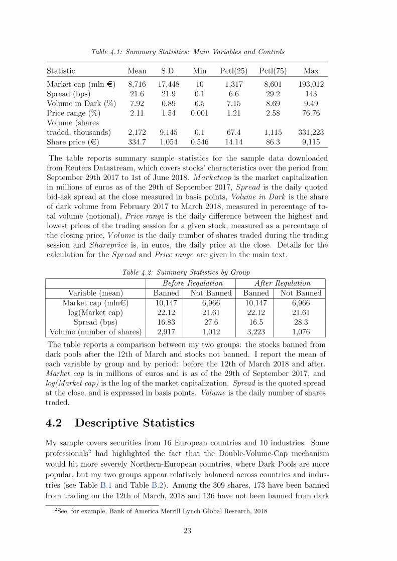
Table 4.1: Summary Statistics: Main Variables and Controls
Statistic Mean S.D. Min Pctl(25) Pctl(75) Max
Market cap (mln e) 8,716 17,448 10 1,317 8,601 193,012Spread (bps) 21.6 21.9 0.1 6.6 29.2 143Volume in Dark (%) 7.92 0.89 6.5 7.15 8.69 9.49Price range (%) 2.11 1.54 0.001 1.21 2.58 76.76Volume (sharestraded, thousands) 2,172 9,145 0.1 67.4 1,115 331,223Share price (e) 334.7 1,054 0.546 14.14 86.3 9,115
The table reports summary sample statistics for the sample data downloadedfrom Reuters Datastream, which covers stocks’ characteristics over the period fromSeptember 29th 2017 to 1st of June 2018. Marketcap is the market capitalizationin millions of euros as of the 29th of September 2017, Spread is the daily quotedbid-ask spread at the close measured in basis points, Volume in Dark is the shareof dark volume from February 2017 to March 2018, measured in percentage of to-tal volume (notional), Price range is the daily difference between the highest andlowest prices of the trading session for a given stock, measured as a percentage ofthe closing price, V olume is the daily number of shares traded during the tradingsession and Shareprice is, in euros, the daily price at the close. Details for thecalculation for the Spread and Price range are given in the main text.
Table 4.2: Summary Statistics by Group
Before Regulation After RegulationVariable (mean) Banned Not Banned Banned Not Banned
Market cap (mlne) 10,147 6,966 10,147 6,966log(Market cap) 22.12 21.61 22.12 21.61
Spread (bps) 16.83 27.6 16.5 28.3Volume (number of shares) 2,917 1,012 3,223 1,076
The table reports a comparison between my two groups: the stocks banned fromdark pools after the 12th of March and stocks not banned. I report the mean ofeach variable by group and by period: before the 12th of March 2018 and after.Market cap is in millions of euros and is as of the 29th of September 2017, andlog(Market cap) is the log of the market capitalization. Spread is the quoted spreadat the close, and is expressed in basis points. Volume is the daily number of sharestraded.
4.2 Descriptive Statistics
My sample covers securities from 16 European countries and 10 industries. Some
professionals2 had highlighted the fact that the Double-Volume-Cap mechanism
would hit more severely Northern-European countries, where Dark Pools are more
popular, but my two groups appear relatively balanced across countries and indus-
tries (see Table B.1 and Table B.2). Among the 309 shares, 173 have been banned
from trading on the 12th of March, 2018 and 136 have not been banned from dark
2See, for example, Bank of America Merrill Lynch Global Research, 2018
23

Figure 4.1: 5-Day Moving Average of the Spread for my Control and Treatment Groups
The figure displays a 5-day moving average of the quoted spread at the close for the groupof stocks banned from dark dark after the 12th of March 2018 (in blue) and for the stocksnot banned during the entire period (black), from the 3rd of January 2018 to the 1st ofJune 2018.
pools during the whole sample period. Figure 4.1 shows the evolution the spread
for the two groups, before and after the regulation. It is a 5-day backward-looking
moving average around the 12th of March. The first thing we notice is the difference
in average spread between the two groups (16.83 bps and 27.6 bps), which can be
explained by the higher market capitalization of stocks banned from dark pools rela-
tive to the others (10 billion euros and 7 billion euros, respectively) as well as higher
average trading volume before the ban (2,917 shares per day and 1,012 shares per
day respectively). However, while their trends look similar before the regulation, an
irregularity appears on the 12th of March. Table 4.2 reports summary statistics by
group (banned or not banned) before and after the regulation. It shows a decrease
in average spread between the two periods for stocks banned from dark pools (by
around 2%) and an increase for stocks not banned from dark pools (by more than
4%). Figure 4.2 shows a comparison between their change in spread before and after
the regulation, with a kernel density estimation of their distribution. The median
change for the stocks banned from dark pool has been a decrease in 4% in average
spread between the two periods, while the median change in spread for the control
group is an increase of 0.6%. Those statistics, altogether with Figures 4.1 and 4.2
point at a positive impact on spreads of the ban.
4.3 Identification Strategy
When studying the impact of dark trading on liquidity, an obvious challenge is
endogeneity: bad market liquidity can induce traders to send their orders to a
dark pool, where they might find alternative liquidity and a price improvement,
especially when the exchange’s spread is high (Ready (2014)). With the Double-
Volume-Cap mechanism, the threshold of 8% offers a sharp non-linearity in the
treatment of dark trading, and by selecting a sample with a level of dark trading
24

Figure 4.2: The Change in Average Spread Before and After the Ban
The figure displays the distribution of stocks by their change in average spread beforeand after the regulation and by group. The figure displays a kernel estimation (using anEpanechnikov function) of the probability density function of the change by group. Thefigure highlights the median change in each group. The period before the ban spans fromthe 29th of September 2017 to the 11th of March 2018, and the period after the ban spansfrom the 12th of March 2018 to the 1st of June 2018.
around that threshold allows for a fair comparison between the two groups. I argue
that, for a stock, having a dark share of 7.9% or 8.1% is largely random, for at least
two reasons. First of all, it is not in any trader’s interest to change her trading
strategy in order to limit/increase the share of dark trading for a stock. Secondly,
it would also imply that traders have a good estimation of the dark volume for a
stock. However, having a fair estimation of such volume is very complex, given the
fragmentation of the market and the blurry definition of dark trading. One can
imagine that only a regulatory authority with access to data from all trading venues
can fairly estimate a stock’s dark trading volume3. Moreover, the treatment is a
very clean shock to dark trading. Former studies of dark pool regulation required
a two-stage estimation, with a first stage estimating the impact of a regulation on
dark trading. Here, banning stocks from trading in all dark pools, overnight, allows
us to directly estimate the impact of dark trading on liquidity. Finally, the delay in
the implementation of the DVC mechanism compared to other measures implied by
MiFID II allows to get rid of confounding effects due to other new rules. Limits to
the identification strategy are discussed in Section 5.
3Even the ESMA had to delay the ban because it lacked the proper data
25

4.4 Main Specification
I use an unbalanced panel data to regress the spread of each stock on a dummy
equal to one for stocks banned from dark pools after the 12th of March, and equal
to 0 for all other observations. I use firm and time (day) fixed effects. I cluster the
standard errors at the firm level, consistently with most empirical studies (Boneva
et al. (2016), Hendershott et al. (2011)), and estimate
Spreadi,t = αi + δt + β(Dark > 8% ∗ Post Ban)i,t + γx′i,t + εi,t. (4.3)
For each stock i and each day t for the entire period. Dark > 8% is a dummy equal
to one if the share of dark trading for the stock was higher than 8% (that is, subject
to the ban) and Post Ban is equal to one after the 12th of March 2018 (that is,
the period of ban from dark pools). αi is the individual (firm) effect, δt is the time
(day) effect, and x′i,t is a vector of controls (inverse of share price, volume, volatility),
variable across time. This model allows to eliminate bias from unobservable factors
that change over time but are constant over entities and it controls for factors that
differ across entities but are constant over time. The use of firm fixed effect allows
me to take into account the differences between the two groups and to correctly
estimate the impact of the ban on quoted spreads. β is the coefficient of interest,
and we expect it to be negative. The clustering of standard errors allows to take into
account potential heteroskedasdicity and correlation between the error term across
time.
4.5 Alternative Specification
A panel data analysis using fixed effects seems to be the best approach here. How-
ever, it does not allow to estimate the relationship between the bid-ask spread and
some firm-specific characteristics (fixed across time) and markets conditions (day-
specific). However, I argue that this approach is valid as I focus on stocks with
similar level of dark trading, even if it requires the addition of controls to identify
correctly the effect of the ban. If the estimate will be less precise than a regression
with fixed effects, using a difference-in-differences framework allows to estimate the
importance of the controls described above.
I first run the following difference-in-differences regression:
Spreadi,t = θ + µDark > 8%i + ηPost Bant+
β(Dark > 8%i ∗ Post Ban)i,t + x′i,tΓ + εi,t (4.4)
Where θ is the intercept, µ measures the differences between the two groups, η
measures the differences between the two time periods and β evaluates the impact
of dark trading on liquidity. Dark > 8%i is a dummy equal to one if the stock had
a share of dark trading greater than 8% as of the 12th of March (that is, subject
to the ban) and Post Bant is a dummy equal to one after the 12th of March and 0
26

before.
I then run the same regression with two sets of controls, in vector form x′i,t: first as
in Boneva et al. (2016) to account for general market conditions (Stoxx 50 return
index, Stoxx 50 volatility index) and the log of each firm’s market capitalization. I
then add the same controls as in the previous specification: the inverse of the share
price, volume and volatility. Those specifications will shed a light on the impact of
general market conditions on stocks’ liquidity.
The results are presented in the next section.
27

5
Results
5.1 The Impact of Dark Trading on Liquidity
Table 5.1 reports the impact of banning stocks from trading in dark pools on their
quoted bid-ask spread. Regression (1) reports the estimates for the simple panel
data analysis, equation 4.3. Consistent with the prediction from Section 3 and the
notion that a larger share of uninformed trades will execute in the dark, my results
indicate that the spread becomes narrower as a stock is forced to be traded away
from dark venues. The impact of dark trading on spreads in the lit market is negative
across all my specifications and statistically significant across most of my regression
specifications. The magnitude of the increase in quoted spreads is also economically
significant. I report a decrease in spreads of 1.637 basis points for stocks banned
from dark pool. Another way to understand that number is to say that the results
imply, given my assumptions, that a fall in dark trading from 8.5% to zero narrows
the quoted bid-ask spread by 10%. This figure is consistent with Comerton-Forde
and Putnins (2015) who find that increasing dark trading from zero to 10% of dollar
volume is expected to increase quoted spreads by 11% after controlling for other
factors. It contrasts, however, with Foley and Putnins (2016), who find that an
increase in 5% of dark volume narrows the spread by around 2%.
5.2 Robustness Checks
Different Time Periods
I run alternatively the above regression for three time periods:
- The whole period, from September 2017 to June 2018,
- From the 3rd of January to June 2018,
- From the 2nd of March to the 22nd of March 2018.
Comparing the coefficients between the three regressions allows to identify the po-
tential differences between long-term and short-term effect of the regulation. The
results are robust, both in sign and magnitudes, across all time periods (see Table
5.2). They range from -1.158 bps to -1.637 bps, which in percentage terms means a
narrowing of quoted spread by between 7% and 10%. The fact that the coefficient
28

Table 5.1: Panel Data Estimates
Dependent variable:
Spread
(1) (2)
Dark>8%*Post Ban −1.637∗∗∗ −1.534∗∗∗
(0.252) (0.252)
Volatility 39.863∗∗∗
(4.621)
Volume −0.0001∗∗∗
(0.00001)
ISP 8.863∗∗
(3.857)Firm Fixed effect Yes YesDay Fixed Effect Yes Yes
Observations 46,769 46,259R2 0.001 0.003Adjusted R2 −0.009 −0.007F Statistic 42.363∗∗∗ (df = 1; 46302) 31.819∗∗∗ (df = 4; 45789)
Note: ∗p<0.1; ∗∗p<0.05; ∗∗∗p<0.01
This table reports regression estimates using a stock-day panel in which thedependent variable is the quoted spread at the close. The key independentvariable is a dummy equal to 1 for stocks banned from dark pools. Controls:V olatility is measured by the price range as a percentage of closing price,V olume is the daily turnover by volume measured by the number of sharestraded; ISP is the inverse of the closing share price. R2 excludes the varianceexplained by the fixed effects. Standard errors are clustered by stocks andstandard errors are reported in parentheses. The period considered spans fromthe 29th of September 2017 to the 1st of June 2018.
29

Table 5.2: Panel Data Estimates by Time Period: Summary
Dependent variable:
Spread
All period 2018 only 20-day period
Dark>8%*Post Ban −1.637∗∗∗ −1.247∗∗∗ −1.158∗
(0.252) (0.294) (0.600)
Firm Fixed effect Yes Yes YesDay Fixed Effect Yes Yes Yes
Observations 46,769 30,523 6,834R2 0.001 0.001 0.001Adjusted R2 −0.009 −0.013 −0.050F Statistic 42.363∗∗∗ 18.024∗∗∗ 3.716∗
(df = 1; 46302) (df = 1; 30111) (df = 1; 6504)
Note: ∗p<0.1; ∗∗p<0.05; ∗∗∗p<0.01
This table reports regression estimates using a stock-day panel in which thedependent variable is the quoted spread at the close. The key independentvariable is a dummy equal to 1 for stocks banned from dark pools. R2 excludesthe variance explained by the fixed effects. Standard errors are clustered atthe firm level and are reported in parentheses. Periods are defined in themain text.
is higher in absolute value when I consider the entire period might imply that there
have been medium-term effects not captured by the 20-day period regression.
Addition of Controls
I follow Hendershott et al. (2011) by adding as controls the inverse of the share
price, the volatility computed as in Parkinson (1980) and the turnover by volume.
Those controls take into account the impact of firm-specific changes over time. The
controls suggest that the spread increases in volatility (as predicted by Zhu (2014)),
decreases in traded volume and with the share price. The impact of volatility is
substantial: an increase in 1% in the price range (representing half of the average
price range) increases, on average, the spread by 39 bps (the spread more than
doubles). Intuitively, we can think of volatility as a measure of risk, and higher risk
makes the market maker more reluctant to hold the asset, and asks for a higher
reward in order to be willing to enter transactions (McInish and Wood (1992)). The
positive coefficient for the Inverse of the Share Price implies that spreads narrow
as the stock price increases, or, conversely, liquidity worsens when the stock price
falls. Gennotte and Leland (1990) show that during crashes, market makers revise
down their expectations and are less willing to absorb the demand for liquidity. The
coefficient on volume, although statistically significant, is small: it implies that an
increase by 10% in volume (an increase by 200 shares on average) will translate into a
30

spread narrowing of 0.1%. Those coefficients are robust, both in sign and magnitude,
across the three time periods I consider. The standard errors are cluster-robust at
the firm level.
Do Large Stocks Respond Less to Dark Trading?
Several empirical studies (Menkveld et al. (2017) for instance) have highlighted the
difference in responses from small and large capitalizations to dark trading. I sort
stocks into quartiles based on market capitalization (Q1 contain the 25% smallest
stocks and Q4 the 25% largest) and run regression 4.3 on each group. Estimates are
reported in Table 5.4. The second and fourth quartiles do not exhibit major dif-
ferences, with a spread response to the ban of, respectively, 3 and 2.6 basis points,
representing a narrowing in spread of 13% and 20%. My results tend, indeed, to
point at a larger response from large market capitalizations. In contradiction with
previous findings, the smallest market capitalizations do not respond more than
large market capitalizations to dark trading, with an average response to the ban
of -1.86 bps, or -5.4%. Finally, stocks in the third quartile exhibit an increase in
spread following the regulation, of more than 4%.
A possible explanation is the larger size of my sample compared to other studies:
Comerton-Forde and Putnins (2015) study a sample with an average market capi-
talization of around 1 billion dollars (890 million euros), Degryse et al. (2015) have
an average of 8 million euros, while mine has an average of 8.7 billion euros. I may
not have enough small very small stocks to derive conclusions about the impact of
a stock’s size on its response to dark trading.
As a whole, my results show that, consistently with my model’s prediction, ban-
ning stocks from trading in dark pools has narrowed their spread. On average, a
decrease in dark trading, measured as percentage of total notional trading volume,
from 8.5% to zero has improved the spread by between 7 and 10%, a result very close
to that of Comerton-Forde and Putnins (2015). However, I do not find a significant
evidence that stocks with a large market capitalization are less impacted by dark
trading. Finally, I find that the bid-ask spread increases in the stock’s volatility,
and decreases in market capitalization and share price.
5.3 Alternative Specification: the Role of General
Market Conditions
The results of the difference-in-differences regressions are reported in Table 5.4.
Regression (3) allows me to evaluate the impact of general market conditions on
stocks’ bid-ask spread. It appears that volatility significantly increases the spread,
which is consistent with Boneva et al. (2016), Comerton-Forde and Putnins (2015),
McInish and Wood (1992) and Zhu (2014)’s predictions. The estimates (between
0.09 and 0.1) indicate that an increase in market-wide volatility of 6% translates into
an increase in spread of 0.4%. The stock-specific volatility has a substantially larger
31

Table 5.3: Panel Data Estimates by Market Capitalization
Dependent variable:
Spread
Q1 (smallest) Q2 Q3 Q4 (largest)
Dark>8%*Post Ban −1.859∗∗ −3.061∗∗∗ 0.7618∗∗ −2.591∗∗∗
(0.007) (0.005) (0.004) (0.003)
Firm Fixed effect Yes Yes Yes YesDay Fixed Effect Yes Yes Yes Yes
Observations 11,615 11,559 11,638 11,649R2 0.001 0.003 0.0003 0.006Adjusted R2 −0.020 −0.017 −0.020 −0.015F Statistic 6.320∗∗ 36.277∗∗∗ 3.971∗∗ 65.243∗∗∗
df (1; 11377) (1; 11325) (1; 11405) (1; 11415)
Note: ∗p<0.1; ∗∗p<0.05; ∗∗∗p<0.01
This table reports regression estimates using a stock-day panel in which thedependent variable is the quoted spread at the close. I report four regressionsresults, one by each quartile of my sample, defined by the stocks’ market capital-ization. The key independent variable is a dummy equal to 1 for stocks bannedfrom dark pools and equal to 0 for stocks not banned and for all stocks beforethe regulation. R2 excludes the variance explained by the fixed effects. Standarderrors are clustered at the firm level and are reported in parentheses. The periodconsidered spans from the 29th of September 2017 to the 1st of June 2018.
effect: an increase of the price range of 50% increases the spread by almost five times.
The market capitalization is a key determinant of a stock’s bid-ask spread, a finding
shared by most empirical studies. This can be due to the relatively lower volatility
of large capitalization stocks, as well as their higher trading volume. Finally, my
results indicate a positive relationship (although not significant) between the spread
and the Stoxx 50 returns, inconsistently with the aforementioned studies and with
Gennotte and Leland (1990)’s intuition.
32

Tabl
e5.4
:D
iffer
ence
-in
-Diff
eren
ces
Est
imate
s
Dep
ende
nt
vari
able
:
Spre
ad
(1)
(2)
(3)
Dar
k>
8%*P
ost
Ban
−1.
058∗∗
−1.
093∗∗∗
−1.
376∗∗∗
(0.4
13)
(0.3
90)
(0.3
16)
log(
Mkt
cap)
−4.
865∗∗∗
−5.
258∗∗∗
(0.0
64)
(0.0
64)
Vol
atilit
y11
7.54
1∗∗∗
(5.1
97)
Inve
rse
ofShar
eP
rice
0.89
9(0
.633
)V
olum
e−
0.00
002∗∗
(0.0
0001
)Sto
xx
retu
rn0.
001
0.00
2(0
.004
)(0
.003
)Sto
xx
vol
0.10
1∗0.
092∗∗
(0.0
52)
(0.0
42)
Con
stan
t27
.595∗∗∗
130.
503∗∗∗
131.
867∗∗∗
(0.1
84)
(6.5
80)
(5.4
82)
Dar
kvo
l>
8%(D
um
my)
Yes
Yes
Yes
Pos
tM
arch
12th
(Dum
my)
Yes
Yes
Yes
Cou
ntr
yof
orig
inN
oN
oY
esIn
dust
ryN
oN
oY
es
Obse
rvat
ions
46,7
6946
,769
46,2
59R
20.
064
0.16
80.
443
Adju
sted
R2
0.06
40.
168
0.44
3R
esid
ual
Std
.E
rror
21.2
16(d
f=
4676
5)19
.999
(df
=46
762)
16.1
13(d
f=
4622
5)F
Sta
tist
ic1,
063.
671∗∗∗
(df
=3;
4676
5)1,
576.
452∗∗∗
(df
=6;
4676
2)1,
114.
989∗∗∗
(df
=33
;46
225)
Not
e:∗ p<
0.1;∗∗
p<
0.05
;∗∗∗ p<
0.01
33

5.4 Where Have the Dark Volumes Gone?
Regulatory changes are generally regarded by the market as being pro-exchange in
their effects. In particular, the limits on dark trading were expected to drive volumes
back into the lit markets (typically, the exchanges). However, significant concerns
raised concerning the competition between exchanges and Systematic Internalisers
after MiFID II. A Systematic Internaliser (SI) is a MiFID I construct, which was
likely to be more important in MiFID II. It is a bank-owned platform which provides
trading against proprietary capital. SIs provide pre and post trade transparency.
In the middle of 2017 there was a significant concern about SIs usurping the main
trading venues. The argument was that SIs would probably end up connecting to
each other, building an alternative pool of liquidity to the traditional lit market. A
key part of this was that SIs, unlike regulated exchanges, were not subject to the
tick size regime, and could offer to execute at a fraction of a percent better price
than exchanges, and be preferred by algorithms looking for the best price available.
The ESMA launched a consultation aimed at clarifying the SI regime and claimed
that:
It is doubtful that such an outcome would go hand in hand with real ben-
efits for end clients. While it would result in marginally better prices,
it would at the same time undermine the overall quality of the liquid-
ity available, the efficient valuation of equity instruments as well as the
efficient pricing of instruments traded1.
They also clarified that SIs would be subject to the same tick size regime as regular
exchanges. That argument, combined with the development of auctions by lit plat-
forms (which resembles dark trading) made the outcome of MiFID II on the market
structure very unclear.
I investigate the dynamics of the equity market structure in response to regulatory
changes and market conditions: I naively regress the market share of different trad-
ing venue categories on a dummy for MiFID II (equal to 1 after the 3rd of January
and 0 before) and a dummy for the implementation of the ban from dark pools
(equal to 1 after the 12th of March and 0 before) and a set of controls (Stoxx 50
volatility and return indices). Estimates must be interpreted carefully, as the use
of certain types of trading venues might increase the volatility of European markets
overall. The results are just shown as an estimation of the relationship between the
equity market structure, regulatory changes and general market conditions. Consis-
tently with findings from Menkveld et al. (2017), I find a significant increase in lit
exchanges’ market share when volatility is higher. It is the only significant impact
of volatility across types of trading venues. I find a decrease in Auctions’ market
share when the returns increase. The rationale behind is straightforward: when the
price of a stock falls too much during a specific trading day, trading in that stock is
paused and buy and sell orders are cleared in an auction process2.
1Amendments to Commission Delegated Regulation (EU) 2017/2018 (RTS 1) ESMA 70-156-2752There is no harmonized threshold to trigger a trading halt, see ESMA’s Guidelines on the
calibration of circuit breakers and the publication and reporting of trading halts under MiFID II
34

Table 5.5: The Relationship Between the Market Share by Trading Venue Cat-egories and the Regulation (Selected Categories)
Dependent variable:
Market share (%)
SIs Dark Lit
DVC 2.830∗∗∗ −1.693∗∗∗ −2.012(0.944) (0.189) (1.280)
MiFID 26.034∗∗∗ −1.194∗∗∗ −10.591∗∗∗
(1.093) (0.219) (1.481)
Stoxx return −0.018 0.002 0.0004(0.018) (0.004) (0.024)
Stoxx vol −0.377 0.048 0.556∗
(0.230) (0.046) (0.312)
Constant 33.162 2.570 46.744(26.935) (5.389) (36.499)
Observations 148 148 148R2 0.881 0.631 0.396Adjusted R2 0.877 0.621 0.379Residual Std. Error (df = 143) 4.606 0.921 6.241F Statistic (df = 4; 143) 263.511∗∗∗ 61.132∗∗∗ 23.401∗∗∗
Note: ∗p<0.1; ∗∗p<0.05; ∗∗∗p<0.01
This table reports OLS regression estimates using a panel in which thedependent variable is the market share, measured by notional amount. Ireport three regressions results, one for each trading venue category thatI am interest in. The key independent variables are: MiFID, a dummyequal to 1 after the 3rd of January 2018 and 0 before; DVC a dummyequal to 1 after the 12th of March 2018 and 0 before; Stoxx return, theStoxx 50 return index; Stoxx vol the Stoxx 50 volatility index. Standarderrors are clustered at the firm level and are reported in parentheses. Theperiod considered spans from the 1st of November 2017 to the 1st of June2018.
Table 5.5 reports the impact of MiFID II and the Double-Volume-Cap mecha-
nism on the fragmentation of the European equity markets. The DVC mechanism
has hit dark pools, but, interestingly, lit exchanges as well. Figure 5.1 shows the
evolution of the market share by trading venue category. In its 2018 Markets and
Risks Outlook, the French Financial Markets Authority (Autorite des Marches Fi-
nanciers, AMF) criticized MiFID II and the DVC mechanism for, as feared before
from 2017
35

their implementation, the rapid rise in market share of SIs, which was almost nonex-
istent in November 2017 and accounted for almost 30% of total trading volume (in
notional) in January 2018. My naive regression results estimate at 26% the rise
in their market share due to the implementation of MiFID II, volume coming no-
tably from Lit exchanges (loss in 11%) and other forms of OTC trading (-12%, see
Table B.9 in Appendix B). Those coefficients are statistically significant at the 1%
level. The DVC mechanism, implemented with a delay, has had no significant effect
on exchanges’ market share, but, as expected, hit dark pools (-1.7%). Auctions
(+1.2%) and SIs (+2.8%) are the main beneficiaries. The impact that Systematic
Internalisers might have on the bid-ask spread is hard to predict. Their specificity
is that they do not rely on trading fees, but make money out of the spread. If they
are tempted to offer a slight price improvement to attract algorithmic traders, it is
hard to believe that their inventory depth can allow them to sustain better prices
than a whole exchange. The mechanism behind their rise remains to be explored.
By facilitating the development of SIs, MiFID II and the DVC mechanism failed at
making the equity market structure more exchange-based and less fragmented.
5.5 Limits and Possible Extensions
My empirical analysis requires to make some assumptions. First of all, I need to
assume that the effect that I have been trying to seize is due to the ban from dark
pools, and not due to changes in market fragmentation, and in particular the rise in
Systematic Internalisers. In a broad sense, SIs belong to the off-exchange trading,
but is still considered lit. Their impact on liquidity is yet to be determined, and
could thus bias my estimates (either upwards or downwards). Moreover, my measure
of dark trading is an average over twelve months and does not tell anything about
the trend. It does not allow me to infer the actual level of dark trading at the time of
the ban from dark pools. In order to make my results relevant, I need to assume that
the level of dark trading at the time of the regulation was similar to their twelve-
month average. Considering the fall in dark trading due to the implementation of
MiFID II on the 3rd of January, one could argue that there has been an anticipation
effect due to the implementation of all other measures. I argue, here, that given
the trend of dark pool’s market share between the beginning of 2018 and the 12th
of March (relatively constant and almost back to its original level after one week,
see Figure 5.1), it is reasonable to assume that the dark share for my sample has
remained constant. Moreover, it would only bias my estimates downward, and make
my results more conservative.
A second limit of my analysis lies in the quality of the data used: contrarily to
the United States, there is no unified framework for aggregating financial markets
data in Europe. Moreover, the data used is at the day level: other measures of the
bid-ask spread require order-level data and might yield different empirical results.
Finally, and more generally, my study focuses on only one measure of market quality.
My findings do not say anything about the price discovery process, and not allow
36

Figure 5.1: The Evolution of the Equity Trading’s Landscape: Market Share by TradingVenue Category
The figure shows the daily market share, measured as a percentage of total notional volumeof trading in Europe, of different trading venue categories, from the 1st of November 2017to the 1st of June 2018. The red line corresponds to the first wave of bans from dark poolsas part of the Double-Volume-Cap mechanism (12th of March 2018), and the dotted blackline corresponds to the implementation of MiFID II (3rd of January 2018).
me to infer conclusions about overall investors’ welfare.
37

6
Conclusion
Technological advances and regulatory changes have permitted the development of
Multilateral-Trading-Facilities in Europe. Among them, dark pools have attracted
a special attention: by removing pre-trade transparency and offering potential price
improvement, they are more likely to attract uninformed investors and widen the
spread of the reference lit exchange. A simple model of spread determination in
a market where a dark pool operates alongside a regular stock exchange run by a
risk-neutral market maker allows me to highlight that mechanism.
However, trying to evaluate the impact of dark trading on liquidity is limited by
endogeneity issues. By banning a large amount of stocks from dark trading when
their share of trading in the dark is greater than 8%, MiFID II’s Double-Volume-Cap
mechanism provides an ideal framework to identify the effect of dark pool on equity
markets’ liquidity. My results show that banning stocks from trading in the dark
has narrowed their bid-ask spread by around 10%, and are robust across several
specifications. In contradiction with previous literature, I do not find evidence that
small capitalizations are more effected by dark trading. I also document the fact
that Systematic Internalisers, rather than regular stock exchanges, have benefited
from the regulation. Their impact on market quality, both on a theoretical and
empirical point of view, remains largely unexplored.
Future research could focus on different measures of liquidity as well as other di-
mensions of market quality, and on the impact of the rapid expansion of SIs. On the
theoretical side, developing a dynamic model of spread determination in a market
where a dark pool and a regular exchange operate alongside could reach different
conclusions, as informed traders might not want to reveal their private information
by trading on the lit exchange.
38

Bibliography
S. Alizadeh, M. W. Brandt, and F. X. Diebold. Range-based estimation of stochastic
volatility models. The Journal of Finance, 57(3):1047–1091, 2002.
Y. Amihud and H. Mendelson. Dealership market: Market-making with inventory.
Journal of Financial Economics, 8(1):31–53, 1980.
W. Bagehot. The only game in town. Financial Analysts Journal, 27(2):12–14, 1971.
H. Bessembinder. Trade execution costs and market quality after decimalization.
Journal of Financial and Quantitative Analysis, 38(4):747–777, 2003.
L. Boneva, O. Linton, and M. Vogt. The effect of fragmentation in trading on market
quality in the uk equity market. Journal of Applied Econometrics, 31(1):192–213,
2016.
S. Buti, B. Rindi, and I. M. Werner. Dark pool trading strategies, market quality
and welfare. Journal of Financial Economics, 124(2):244–265, 2017.
C. Comerton-Forde and T. J. Putnins. Dark trading and price discovery. Journal
of Financial Economics, 118(1):70–92, 2015.
C. Comerton-Forde, K. Malinova, and A. Park. Regulating dark trading: Order
flow segmentation and market quality. Journal of Financial Economics, 130(2):
347–366, 2018.
T. E. Copeland and D. Galai. Information effects on the bid-ask spread. the Journal
of Finance, 38(5):1457–1469, 1983.
F. De Jong and B. Rindi. The microstructure of financial markets. Cambridge
University Press, 2009.
H. Degryse, M. Van Achter, and G. Wuyts. Dynamic order submission strategies
with competition between a dealer market and a crossing network. Journal of
Financial Economics, 91(3):319–338, 2009.
H. Degryse, F. De Jong, and V. v. Kervel. The impact of dark trading and visible
fragmentation on market quality. Review of Finance, 19(4):1587–1622, 2015.
D. Easley and M. O’hara. Price, trade size, and information in securities markets.
Journal of Financial economics, 19(1):69–90, 1987.
39

S. Fioravanti and M. Gentile. The impact of market fragmentation on european stock
exchanges. Commissione Nazionale per le Societa e la Borsa Working Paper, 69,
2011.
S. Foley and T. J. Putnins. Should we be afraid of the dark? dark trading and
market quality. Journal of Financial Economics, 122(3):456–481, 2016.
M. B. Garman. Market microstructure. Journal of financial Economics, 3(3):257–
275, 1976.
G. Gennotte and H. Leland. Market liquidity, hedging, and crashes. The American
Economic Review, pages 999–1021, 1990.
L. R. Glosten and L. E. Harris. Estimating the components of the bid/ask spread.
Journal of financial Economics, 21(1):123–142, 1988.
L. R. Glosten and P. R. Milgrom. Bid, ask and transaction prices in a specialist
market with heterogeneously informed traders. Journal of financial economics, 14
(1):71–100, 1985.
C. Gresse et al. Effects of the competition between multiple trading platforms on
market liquidity: evidence from the mifid experience. SSRN eLibrary, 2011.
T. Hendershott and H. Mendelson. Crossing networks and dealer markets: Compe-
tition and performance. The Journal of Finance, 55(5):2071–2115, 2000.
T. Hendershott, C. M. Jones, and A. J. Menkveld. Does algorithmic trading improve
liquidity? The Journal of Finance, 66(1):1–33, 2011.
J. Hengelbrock and E. Theissen. Fourteen at one blow: The market entry of
turquoise. Available at SSRN 1743589, 2009.
A. Kwan, R. Masulis, and T. H. McInish. Trading rules, competition for order
flow and market fragmentation. Journal of Financial Economics, 115(2):330–348,
2015.
A. S. Kyle. Continuous auctions and insider trading. Econometrica: Journal of the
Econometric Society, pages 1315–1335, 1985.
A. Madhavan. Market microstructure: A survey. Journal of financial markets, 3(3):
205–258, 2000.
T. H. McInish and R. A. Wood. An analysis of intraday patterns in bid/ask spreads
for nyse stocks. the Journal of Finance, 47(2):753–764, 1992.
A. J. Menkveld, B. Z. Yueshen, and H. Zhu. Shades of darkness: A pecking order
of trading venues. Journal of Financial Economics, 124(3):503–534, 2017.
M. Mizen. Effective spreads in european equities. TABB Group pinpoint, 2010.
40

M. O’hara. Market microstructure theory, volume 108. Blackwell Publishers Cam-
bridge, MA, 1995.
M. Parkinson. The extreme value method for estimating the variance of the rate of
return. Journal of business, pages 61–65, 1980.
O. Petrenko. Understanding the eu’s approach to harmonised regulatory reporting.
Journal of Securities Operations & Custody, 8(4):311–321, 2016.
M. Petrescu and M. Wedow. Dark pools in european equity markets: emergence,
competition and implications. ECB Occasional Paper, (193), 2017.
M. Ready. Determinants of volume in dark pool crossing networks. In AFA 2010
Atlanta Meetings Paper, 2014.
R. Roll. A simple implicit measure of the effective bid-ask spread in an efficient
market. The Journal of finance, 39(4):1127–1139, 1984.
A. B. Schmidt. Financial markets and trading: an introduction to market mi-
crostructure and trading strategies, volume 637. John Wiley & Sons, 2011.
H. R. Stoll. The supply of dealer services in securities markets. The Journal of
Finance, 33(4):1133–1151, 1978.
H. R. Stoll. Presidential address: friction. The Journal of Finance, 55(4):1479–1514,
2000.
J. Vaananen. Dark Pools and High Frequency Trading For Dummies. For Dummies,
2014.
L. Ye. Understanding the impacts of dark pools on price discovery. Available at
SSRN 2874957, 2016.
M. Ye. A glimpse into the dark: Price formation, transaction cost and market share
of the crossing network. Transaction Cost and Market Share of the Crossing
Network (June 9, 2011), 2011.
H. Zhu. Do dark pools harm price discovery? The Review of Financial Studies, 27
(3):747–789, 2014.
41

Appendix A
Appendix: Model
A.0.1 Existence and Uniqueness of the Equilibrium
We have:
S =2ασ
2α + (1− α)(2−G(1− S2σ
))
Solving for G(.) gives us:
G(1− S
2σ) =
2(S − ασ)
S(1− α)
Does that equality have a solution, and if yes, is it unique? By definition, G′(.) > 0
and 1− S2σ
is decreasing in S, thus G(.) is strictly decreasing in S.
What about 2(S−ασ)S(1−α) ?
d2(S−ασ)S(1−α)
dS=
2S − 2(S − ασ)
S2(1− α)
Which simplifies to ασ)S2(1−α) > 0.
Now we are sure that if both functions cross at some point, it will be at a unique
point. We have to make sure that they cross on S’ support, [0, σ]:
limS→0
G(1) > 0 > limS→0
2(S − ασ)
S(1− α)= −∞
And
limS→σ
G(0) = 0 < limS→σ
2(S − ασ)
S(1− α)= 2
Which demonstrates existence and uniqueness of the equilibrium.
A.0.2 Proof That β = γ2−γ
In equilibrium, β must be such that informed traders are indifferent between the
two venues:
σ − S = r−σ
42

The equation can be rewritten as:
1− S
σ= r−
Replacing with their true expressions:
(1− α)(1− γ)
α(1− β) + (1− α)(1− γ)=
12(1− α)γ
12(1− α)γ + αβ
As both denominators are strictly greater than 0:
α(1− β) + (1− α)(1− γ)
(1− α)(1− γ)=
12(1− α)γ + αβ
12(1− α)γ
Developing:(1− β)α
(1− α)(1− γ)+ 1 = 1 +
βα12(1− α)γ
Dividing both sides by α:
1
(1− α)(1− γ)− β
(1− α)(1− γ)=
β12(1− α)γ
Rearranging:
1
(1− α)(1− γ)= β(
1
(1− α)(1− γ)+
112(1− α)γ
)
Multiplying both sides by (1− α)(1− γ):
1 = β(12(1− α)γ + (1− α)(1− γ)
12(1− α)γ
)
Isolating β and expressing the right-hand-side in terms of γ:
β = γ(12(1− α)
12(1− α)γ + (1− α)(1− γ)
)
Getting rid of the (1− α):
β = γ(12
12γ + (1− γ)
)
Which gives:
β =γ
2− γAnd, as γ < 1:
β < γ
43

A.0.3 Proof of Sufficiency of β < γ
For the spread to always increase with a dark pool, we need to prove that:
ασ <α(1− β)
α(1− β) + (1− α)(1− γ)σ
Dividing both sides by σα:
1− (1− β)
α(1− β) + (1− α)(1− γ)< 0
Developing:α(1− β) + (1− α)(1− γ)− (1− β)
α(1− β) + (1− α)(1− γ)< 0
As the denominator is always positive, after simplification, we are left with:
(1− γ)(1− α) < (1− α)(1− β)
Which is equivalent to:
β < γ
Which is always true.
44

Appendix B
Appendix: Empirics
Figure B.1: Stoxx 50 Return and Volatility Indices Over the Period (Basis 100 on the 29thof September, 2017)
45

Table B.1: Summary Statistics: Country of Origin
Country Stocks Of which: treated
Austria 5 3Belgium 8 5Denmark 5 2Finland 12 8France 39 14Germany 47 21Ireland 6 5Italy 39 23Luxembourg 2 1Netherlands 17 9Norway 9 4Portugal 4 3Spain 9 6Sweden 43 28Switzerland 15 6United Kingdom 49 35Total 309 173
Table B.2: Summary Statistics: Industries
Industry Stocks Of which: treated
Basic Materials 23 16Consumer Goods 39 23Consumer Services 42 24Financials 63 36Healthcare 16 8Industrials 75 42Oil and Gas 9 4Technology 19 3Telecoms 8 7Utilities 15 10Total 309 173
46

Table B.3: Panel Data Estimates (All Period)
Dependent variable:
Spread
(1) (2)
Dark>8%*Post Ban −1.637∗∗∗ −1.534∗∗∗
(0.252) (0.252)
Volatility 39.863∗∗∗
(4.621)
Volume −0.0001∗∗∗
(0.00001)
ISP 8.863∗∗
(3.857)Firm Fixed effect Yes YesDay Fixed Effect Yes Yes
Observations 46,769 46,259R2 0.001 0.003Adjusted R2 −0.009 −0.007F Statistic 42.363∗∗∗ (df = 1; 46302) 31.819∗∗∗ (df = 4; 45789)
Note: ∗p<0.1; ∗∗p<0.05; ∗∗∗p<0.01
This table reports regression estimates using a stock-day panel in which thedependent variable is the quoted spread at the close. The key independentvariable is a dummy equal to 1 for stocks banned from dark pools and equalto 0 for stocks not banned, and all stocks before the regulation. Controls:V olatility is measured by the price range as a percentage of closing price,V olume is the daily turnover by volume measured by the number of sharestraded; ISP is the inverse of the closing share price. R2 excludes the varianceexplained by the fixed effects. Standard errors are clustered by stocks andare reported in parentheses. The period considered spans from the 29th ofSeptember 2017 to the 1st of June 2018.
47

Table B.4: Panel Data Estimates (2018 Only)
Dependent variable:
Spread
(1) (2)
Dark>8%*Post Ban −1.247∗∗∗ −1.221∗∗∗
(0.294) (0.294)
Volatility 35.655∗∗∗
(5.607)
Volume −0.00004∗∗
(0.00002)
ISP 7.313(5.829)
Firm Fixed effect Yes YesDay Fixed Effect Yes Yes
Observations 30,523 30,179R2 0.001 0.002Adjusted R2 −0.013 −0.012F Statistic 18.024∗∗∗ (df = 1; 30111) 15.610∗∗∗ (df = 4; 29764)
Note: ∗p<0.1; ∗∗p<0.05; ∗∗∗p<0.01
This table reports regression estimates using a stock-day panel in which thedependent variable is the quoted spread at the close. The key independentvariable is a dummy equal to 1 for stocks banned from dark pools and equalto 0 for stocks not banned, and all stocks before the regulation. Controls:V olatility is measured by the price range as a percentage of closing price,V olume is the daily turnover by volume measured by the number of sharestraded; ISP is the inverse of the closing share price. R2 excludes the varianceexplained by the fixed effects. Standard errors are clustered by stocks and arereported in parentheses. The period considered spans from the 3rd of January2018 to the 1st of June 2018.
48

Table B.5: Panel Data Estimates (20-Day Period)
Dependent variable:
Spread
(1) (2)
Dark>8%*Post Ban −1.158∗ −1.118∗
(0.600) (0.605)
Volatility 17.429(13.096)
Volume −0.00003(0.00005)
ISP −38.170(24.260)
Firm Fixed effect Yes YesDay Fixed Effect Yes Yes
Observations 6,834 6,768R2 0.001 0.001Adjusted R2 −0.050 −0.050F Statistic 3.716∗ (df = 1; 6504) 1.825 (df = 4; 6435)
Note: ∗p<0.1; ∗∗p<0.05; ∗∗∗p<0.01
This table reports regression estimates using a stock-day panel inwhich the dependent variable is the quoted spread at the close. Thekey independent variable is a dummy equal to 1 for stocks bannedfrom dark pools and equal to 0 for stocks not banned, and all stocksbefore the regulation. Controls: V olatility is measured by the pricerange as a percentage of closing price, V olume is the daily turnover byvolume measured by the number of shares traded; ISP is the inverseof the closing share price. R2 excludes the variance explained by thefixed effects. Standard errors are clustered by stocks and are reportedin parentheses. The period considered spans from the 2nd of March2018 to the 22nd of March 2018.
49

Figure B.2: Change in Spread by log(Market Cap) and Volatility in (%)
The figures above show the change in average spread before and after the regulation asa function of volatility (price range as a percentage of closing price, details are in themain text) and the log of the market capitalization (in millions euros, as of the 29th ofSeptember 2017). The red line is the prediction of a naive regression of the change inspread on the characteristic.
50

Tabl
eB
.6:
Diff
-in
-diff
Est
imate
s(A
llP
erio
d)
Dep
ende
nt
vari
able
:
Spre
ad2
(1)
(2)
(3)
Dar
k>
8%*P
ost
Ban
−1.
058∗∗
−1.
093∗∗∗
−0.
900∗∗
(0.4
13)
(0.3
90)
(0.3
85)
Sto
xx
retu
rn0.
001
0.00
4(0
.004
)(0
.004
)Sto
xx
vol
0.10
1∗0.
105∗∗
(0.0
52)
(0.0
51)
log(
Mkt
cap)
−4.
865∗∗∗
−4.
525∗∗∗
(0.0
64)
(0.0
68)
ISP
−3.
619∗∗∗
(0.6
63)
Vol
um
e−
0.00
01∗∗∗
(0.0
0001
)V
olat
ilit
y99
.036∗∗∗
(6.1
67)
Con
stan
t27
.595∗∗∗
130.
503∗∗∗
115.
703∗∗∗
(0.1
84)
(6.5
80)
(6.5
66)
Dar
kvo
l>
8%(D
um
my)
Yes
Yes
Yes
Pos
tM
arch
12th
(Dum
my)
Yes
Yes
Yes
Cou
ntr
yof
orig
inN
oN
oY
esIn
dust
ryN
oN
oY
es
Obse
rvat
ions
46,7
6946
,769
46,2
59R
20.
064
0.16
80.
443
Adju
sted
R2
0.06
40.
168
0.44
3R
esid
ual
Std
.E
rror
21.2
16(d
f=
4676
5)19
.999
(df
=46
762)
16.1
13(d
f=
4622
5)F
Sta
tist
ic1,
063.
671∗∗∗
(df
=3;
4676
5)1,
576.
452∗∗∗
(df
=6;
4676
2)1,
114.
989∗∗∗
(df
=33
;46
225)
Not
e:∗ p<
0.1;∗∗
p<
0.05
;∗∗∗ p<
0.01
51

Tabl
eB
.7:
Diff
-in
-diff
Est
imate
s(2
018
On
ly)
Dep
ende
nt
vari
able
:
Spre
ad2
(1)
(2)
(3)
Dar
k>
8%*P
ost
Ban
−0.
727
−0.
777∗
−0.
683
(0.4
92)
(0.4
64)
(0.4
57)
Sto
xx
retu
rn−
0.00
020.
004
(0.0
04)
(0.0
04)
Sto
xx
vol
0.16
4∗∗∗
0.18
3∗∗∗
(0.0
57)
(0.0
56)
log(
Mkt
cap)
−4.
831∗∗∗
−4.
530∗∗∗
(0.0
79)
(0.0
84)
ISP
−5.
167∗∗∗
(0.8
28)
Vol
um
e−
0.00
01∗∗∗
(0.0
0001
)V
olat
ilit
y97
.750∗∗∗
(7.5
55)
Con
stan
t27
.476∗∗∗
129.
287∗∗∗
114.
447∗∗∗
(0.2
71)
(7.0
39)
(7.0
46)
Dar
kvo
l>
8%(D
um
my)
Yes
Yes
Yes
Pos
tM
arch
12th
(Dum
my)
Yes
Yes
Yes
Cou
ntr
yof
orig
inN
oN
oY
esIn
dust
ryN
oN
oY
es
Obse
rvat
ions
30,5
2330
,523
30,1
79R
20.
067
0.17
00.
440
Adju
sted
R2
0.06
70.
170
0.44
0R
esid
ual
Std
.E
rror
21.2
57(d
f=
3051
9)20
.056
(df
=30
516)
16.1
82(d
f=
3014
5)F
Sta
tist
ic73
5.96
1∗∗∗
(df
=3;
3051
9)1,
041.
314∗∗∗
(df
=6;
3051
6)71
9.18
4∗∗∗
(df
=33
;30
145)
Not
e:∗ p<
0.1;∗∗
p<
0.05
;∗∗∗ p<
0.01
52

Tabl
eB
.8:
Diff
-in
-diff
Est
imate
s(2
0-D
ay
Per
iod)
Dep
ende
nt
vari
able
:
Spre
ad2
(1)
(2)
(3)
Dar
k>
8%*P
ost
Ban
−1.
702
−1.
607
−1.
657∗
(1.0
35)
(0.9
82)
(0.9
64)
Sto
xx
retu
rn−
0.00
050.
009
(0.0
14)
(0.0
14)
Sto
xx
vol
0.16
30.
145
(0.2
28)
(0.2
24)
log(
Mkt
cap)
−4.
639∗∗∗
−4.
213∗∗∗
(0.1
67)
(0.1
80)
ISP
−3.
014∗
(1.8
05)
Vol
um
e−
0.00
01∗∗∗
(0.0
0003
)V
olat
ilit
y11
5.19
1∗∗∗
(17.
303)
Con
stan
t27
.427∗∗∗
125.
323∗∗∗
101.
552∗∗∗
(0.5
39)
(18.
902)
(18.
962)
Dar
kvo
l>
8%(D
um
my)
Yes
Yes
Yes
Pos
tM
arch
12th
(Dum
my)
Yes
Yes
Yes
Cou
ntr
yof
orig
inN
oN
oY
esIn
dust
ryN
oN
oY
es
Obse
rvat
ions
6,83
46,
834
6,76
8R
20.
070
0.16
40.
434
Adju
sted
R2
0.06
90.
163
0.43
1R
esid
ual
Std
.E
rror
21.2
19(d
f=
6830
)20
.121
(df
=68
27)
16.2
71(d
f=
6734
)F
Sta
tist
ic17
0.98
3∗∗∗
(df
=3;
6830
)22
3.16
8∗∗∗
(df
=6;
6827
)15
6.50
2∗∗∗
(df
=33
;67
34)
Not
e:∗ p<
0.1;∗∗
p<
0.05
;∗∗∗ p<
0.01
53

Tabl
eB
.9:
The
Rel
ati
on
ship
Bet
wee
nth
eM
ark
etS
hare
byT
radin
gV
enu
eC
ate
gori
esan
dth
eR
egu
lati
on
(All
Cate
gori
es)
Dep
ende
nt
vari
able
:
Mar
ket
shar
e(%
,not
ional
amou
nt)
SIs
Dar
kL
itA
uct
ions
OT
C(n
oSI)
Req
ues
tfo
rQ
uot
es
DV
C2.
830∗∗∗
−1.
693∗∗∗
−2.
012
1.20
8∗−
0.40
10.
068∗∗∗
(0.9
44)
(0.1
89)
(1.2
80)
(0.7
21)
(1.7
78)
(0.0
21)
MiF
ID26
.034∗∗∗
−1.
194∗∗∗
−10
.591∗∗∗
−1.
864∗∗
−12
.415∗∗∗
(1.0
93)
(0.2
19)
(1.4
81)
(0.8
34)
(2.0
57)
Sto
xx
retu
rn−
0.01
80.
002
0.00
04−
0.03
0∗∗
0.04
50.
001∗
(0.0
18)
(0.0
04)
(0.0
24)
(0.0
13)
(0.0
33)
(0.0
004)
Sto
xx
vol
−0.
377
0.04
80.
556∗
−0.
284
0.05
20.
006
(0.2
30)
(0.0
46)
(0.3
12)
(0.1
76)
(0.4
33)
(0.0
05)
Con
stan
t33
.162
2.57
046
.744
57.6
65∗∗∗
−39
.089
−1.
164∗
(26.
935)
(5.3
89)
(36.
499)
(20.
561)
(50.
712)
(0.6
40)
Obse
rvat
ions
148
148
148
148
148
105
R2
0.88
10.
631
0.39
60.
087
0.35
80.
120
Adju
sted
R2
0.87
70.
621
0.37
90.
061
0.34
00.
093
Res
idual
Std
.E
rror
4.60
6(d
f=
143)
0.92
1(d
f=
143)
6.24
1(d
f=
143)
3.51
6(d
f=
143)
8.67
1(d
f=
143)
0.10
1(d
f=
101)
FSta
tist
ic26
3.51
1∗∗∗
61.1
32∗∗∗
23.4
01∗∗∗
3.38
8∗∗
19.9
01∗∗∗
4.57
1∗∗∗
df
4;14
34;
143
4;14
34;
143
4;14
34;
143
Not
e:∗ p<
0.1;∗∗
p<
0.05
;∗∗∗ p<
0.01
54