does diversiﬁcation destroy value? evidence from the...

Journal of Financial Economics 63 (2002) 51–77

Does diversification destroy value?Evidence from the industry shocks$

Owen A. Lamonta,*, Christopher Polkb

aGraduate School of Business, University of Chicago and NBER, 1101 E 58th Street,

Chicago, IL 60637, USAbKellogg Graduate School of Management, Northwestern University, Evanston, IL 60208-2001, USA

Received 13 July 2000; accepted 21 February 2001

Abstract

Does corporate diversification reduce shareholder value? Since firms endogenously choose

to diversify, exogenous variation in diversification is necessary to draw inferences about the

causal effect. We examine changes in the within-firm dispersion of industry investment, or

‘‘diversity’’. We find that exogenous changes in diversity, due to changes in industry

investment, are negatively related to firm value. Thus diversification destroys value, consistent

with the inefficient internal capital markets hypothesis. Measurement error does not cause this

finding. We also find that exogenous changes in industry cash flow diversity are negatively

related to firm value. r 2002 Elsevier Science S.A. All rights reserved.

JEL classification: G34

Keywords: Diversified firms; Internal capital markets

1. Introduction

Firms operating in multiple lines of business tend to have lower values thanportfolios of similar focused firms, as shown in Berger and Ofek (1995), Lang and

$We thank Raghuram Rajan, Henri Servaes, Luigi Zingales, an anonymous referee, and seminar

participants at the American Economic Association, the NBER, and University of Chicago for helpful

comments. Lamont gratefully acknowledges support from the Alfred P. Sloan Foundation, the Center for

Research in Securities Prices at the University of Chicago Graduate School of Business, and the National

Science Foundation.

*Corresponding author. Tel.: +1-773-702-6414; fax: +1-773-702-0458.

E-mail addresses: [email protected] (O.A. Lamont), [email protected] (C. Polk).

0304-405X/02/$ - see front matter r 2002 Elsevier Science S.A. All rights reserved.

PII: S 0 3 0 4 - 4 0 5 X ( 0 1 ) 0 0 0 8 9 - 7

Stulz (1994) and Servaes (1996). This diversification discount has two explanations.First, it could be that diversification itself somehow destroys value. Second, it couldbe that diversification and lower value are not causally related, but merely reflectfirms’ endogenous choices. For example, perhaps low value firms choose to diversify,leading to a negative correlation between diversification and value. These twoexplanations are not mutually exclusive; it could be that low value firms choose todiversify, and this diversification lowers their value still further.

A measure of the degree of diversification is the within-firm dispersion of somecharacteristic, or ‘‘diversity’’. If diversification destroys value, and if diversitymeasures diversification, then diversity should be negatively correlated with firmvalue. For example, Berger and Ofek (1995) show that firms operating in unrelatedbusinesses, defined as operating in different two-digit Standard IndustrialClassification (SIC) codes, have lower values than firms operating in relatedbusinesses. Thus diversity in SIC codes is negatively correlated with value. In thispaper, we test whether diversity in a variety of characteristics is negatively related tovalue. We focus specifically on diversity in investment opportunities.

To infer causation, one needs an exogenous instrument for the level of diversity.We use variation in diversity due to variation in industry characteristics. We relatechanges in diversity to changes in value. Our identifying assumption is that thevariation in industry characteristics is exogenous from the point of view of anindividual diversified firm. Using this assumption, we define the exogenous change indiversity as the change due only to changes in industry characteristics. Usingexogenous diversification allows us to study causality rather than correlation.

One specific explanation for the diversification discount is the inefficient internalcapital markets hypothesis: diversified firms invest inefficiently, spending too little ontheir good segments and too much on their bad segments. Berger and Ofek (1995)find that diversified firms overinvest in segments with poor investment opportunities,and that this overinvestment is related to lower firm value. This explanation impliesthat diversity in investment opportunities destroys value, since diversity creates asituation in which the firm can inefficiently transfer funds from good segments tobad segments.

A variety of other evidence supports this cross-subsidization hypothesis. Lamont(1997) finds that when oil prices fall, oil firms lower their investment in non-oilsegments. Shin and Stulz (1998) find that more generally, cash flow in one part of thefirm affects investment in another part of the firm. Scharfstein (1998) testspredictions from Scharfstein and Stein (2000), and finds that diversified firms investtoo much in low Q segments and too little in high Q segments, consistent withintrafirm ‘‘socialism’’. Rajan et al. (2000) present a model where resources flow toinefficient divisions, depending on their size and investment opportunities. Theyexamine segment investment, segment size, and industry Q; and find evidenceconsistent with their theory. They also find that firm value is negatively related todiversity in investment opportunities. We test this last finding of Rajan et al. (2000),and in particular we test for a causal connection between diversity and value.

In addition to endogeneity, measurement error is a major issue when drawinginferences about the effect of diversification. Chevalier (1999) and Whited (2001)

O.A. Lamont, C. Polk / Journal of Financial Economics 63 (2002) 51–7752

study the effects of measurement error, and argue that it explains some of theevidence on the inefficient internal capital markets hypothesis. Measurement error isa particular concern when studying the relation between diversity and excess value,because both the diversity measure and the excess value measure are calculated usingthe same underlying segment and industry data.

For example, diversity in investment opportunities can be measured using thediversity of industry Q’s for each segment. However, the same industry Q’s are alsoused to calculate the dependent variable, excess value. Thus measurement errorpotentially produces a mechanical correlation between the dependent andindependent variable, leading to spurious inferences. For this reason, we measurediversity in investment opportunities using diversity in industry investment, notindustry Q’s. Industry investment should be correlated with industry investmentopportunities, but less correlated with measurement error in industry Q: Since thevariable used to generate diversity is different than the variable used to calculateexcess value, hardwiring is less of a problem. We quantify the potential effect ofmeasurement error, and find it to be small for our baseline specification.

The following example illustrates our empirical strategy of using industry shocksto identify the causal effect of diversity. Consider a diversified firm with two divisionsof equal size, an aircraft division and an electronics division. Suppose the aircraftindustry has much lower investment opportunities than the electronics industry, sothat the firm has a high diversity in investment opportunities. We observe thisdiversity in investment opportunities by observing that focused firms in the aircraftindustry have lower investment than focused firms in the electronics industry.According to the inefficient internal capital markets hypothesis, the diversified firmwill spend too much on its aircraft division and too little on its electronics division,and this misallocation will cause the firm to have low value. Perhaps the firm followsa ‘‘fair’’ rule of splitting the capital expenditures evenly between the two divisions.Now suppose that, due to changing industry conditions, investment opportunities inthe aircraft industry improve. This change will decrease the firm’s diversity ofinvestment opportunities, and as a result the ‘‘fair’’ allocation is less harmful. Thusan exogenous decrease in diversity, caused by industry shocks, leads to a decrease inmisallocation and an increase in relative firm value.

To preview the results, we find that exogenous changes in investment diversity arenegatively related to changes in excess value. Thus the observed diversificationdiscount is not just a consequence of selection biases and endogenous choices byfirms. Further, we show that measurement error is a very unlikely explanation for thenegative effect of exogenous diversity. The contribution of this paper is to show thecausal effect of diversification: diversification destroys value. This finding supportsthe inefficient internal capital markets hypothesis. We also find a negative relationbetween endogenous diversification and value. This finding is more ambiguous, butis consistent with the self-selection hypothesis that firms diversify in response to poorperformance.

We also examine changes in diversity in industry leverage, sales growth, and cashflow. Changes in diversity in these other variables do not subsume exogenouschanges in investment diversity, so in this sense the inefficient internal capital

O.A. Lamont, C. Polk / Journal of Financial Economics 63 (2002) 51–77 53

markets hypothesis survives. We find evidence that cash flow diversity, but notleverage or sales growth diversity, destroys value. Investment diversity does notsubsume cash flow diversity.

We further investigate the inefficient internal capital markets hypothesis byexamining segment investment in diversified firms compared to investment infocused firms. We find that, consistent with the hypothesis, firms smooth investmentacross segments compared to the investment of focused firms in the same industry.Although this specific evidence cannot prove causality, it shows that the availableevidence on segment investment is consistent with the hypothesis that capitalexpenditures are inefficiently allocated within the firm.

This paper is organized as follows. Section 2 describes previous research. Section 3describes the sample and the construction of variables measuring exogenous andendogenous changes in diversity. Section 4 presents results for diversity ininvestment opportunities measured using industry investment. Section 5 exploresdiversity in other industry characteristics, including capital structure, profitability,and sales growth. Section 6 presents conclusions.

2. Previous research

In addition to the inefficient internal capital markets hypothesis, there are manygeneral ways in which unrelatedness might reduce value. It could be that managershave limited expertise and cannot effectively manage diverse businesses, or thatunrelated segments have conflicting operational styles or corporate cultures. Thisbroader explanation also predicts that diversity of characteristics is negativelycorrelated with value.

Other theories predict a positive relation between diversity and value. In Lewellen(1971) diversity of cash flow variation is good if it allows greater tax benefits ofleverage by reducing the volatility of cash flows and the probability of financialdistress. Hadlock et al. (1999) argue that diversity might be good if managers’ privateinformation at the segment level washes out at the firm level, reducing informationasymmetry. Another argument is that diversity in investment opportunities is goodwhen internal capital markets function better than external markets, since itmaximizes the scope of the internal market. Hubbard and Palia (1999) find evidence,using acquisitions in the 1960s, that gains are greatest when a financiallyunconstrained buyer acquires a constrained target. Thus diversity in financialconstraints is good. Fulghieri and Hodrick (1997), Stein (1997), and Wulf (2000) alsodiscuss the possible benefits of diversity.

Value destruction or creation can occur in two ways. The value of any asset is thesum of discounted future cash flows, so that value can change either due to changesin cash flows or changes in discount rates. Lamont and Polk (2001) show that asubstantial fraction of the cross-sectional variance of diversification discounts is dueto variation in expected returns; firms with high expected returns have low values,and firms with low expected returns have high values. Most existing empirical workhas focused on potential cash flow effects of diversification (for example, studies of


profits or productivity in diversified firms). One could also imagine discount rateversions of existing explanations. For example, perhaps inefficient cross-subsidiza-tion involves taking excessively risky projects with high discount rates. We do notattempt to discriminate between these two sources of value destruction in this paper.

A variety of papers examine endogenous changes in diversity, in which firmschoose to diversify (usually through an acquisition) or focus (usually throughspinoffs or divestitures). Lang and Stulz (1994), Hyland (2000), Campa and Kedia(1999), and Graham et al. (1999) all test whether endogenous diversifying behaviorleads to a negative correlation of diversity and value, by studying whether firms havelow value and poor performance before diversifying.

A frequent finding is that refocusing raises firm value, as in Comment and Jarrell(1995) and John and Ofek (1995). Daley et al. (1997) find that spun-off segmentsexperience improved performance, especially if they are unrelated (see also Kaplanand Weisbach, 1992). Gertner et al. (1999) find that the investment of spun-offsegments changes in a way consistent with the inefficient internal capital marketshypothesis. Berger and Ofek (1996, 1999) find that takeovers, leveraged buy-outs,shareholder pressure, managerial turnover, and other largely external sources are thecause of much refocusing. These findings are consistent with the idea thatdiversification destroys value, and that the market for corporate control helpseliminate value-destroying diversification (for related work, see also Schlingemannet al., 1999; Peyer and Shivdasani, 2000).

If the decision to diversify reflects value-destroying managerial waste, one mightexpect endogenous increases in diversity to decrease value. Morck et al. (1990) andMaquiera et al. (1998) find that acquiring firm stockholders lose value in diversifyingacquisitions. Schoar (1999) finds that firms that acquire plants in unrelated industriesexperience a subsequent decrease in total firm productivity. If in contrast, firmsoptimally choose to diversify as in Maksimovic and Phillips (1999) and Fluck andLynch (1999), one might expect all endogenous changes in diversification to have apositive effect, reflecting firms moving closer to the optimum. Of course, sinceendogenous actions are taken in response to events that the econometrician cannotobserve, the observed correlation between endogenous diversification and value thatwe measure can never be conclusive about whether firms are behaving optimally.

3. Sample and variable construction

3.1. Data

Our sample consists of firms reporting segment data in the Compustat Currentand Research database, 1979–1997. The data sources and variables are describedmore fully in the appendix. Following Berger and Ofek (1995), we discard firm-yearswith segments in the financial services industry, total firm sales of less than $20million, or discrepancies in segment and firm data. We also require firms to haveinformation on firm-level equity, debt, investment, capital stock, and sales growth.The only segment level data we use for the main empirical results are sales, assets,


and SIC codes for each individual segment (in Section 4.4 we briefly examinesegment capital expenditures).

Our measure of excess value is based on market-book ratios. Q is the ratio of themarket value of the firm (the market value of common stock plus the book value oftotal assets minus book equity minus deferred taxes) divided by the total book assetsof the firm.1 For each segment of a diversified firm, we find a group of matchingfocused firms with the same two-digit SIC code. We then calculate the median foreach segment’s industry, QIND: We drop every diversified firm that does not have atleast five matching focused firms for each of its segments. We then form %Q; theimputed value ratio, for the entire diversified firm as the weighted average of theindustry QIND’s:

%Q ¼Xn

j¼1

wjQIND j ¼Xn

j¼1

wj median Q1;Q2;y;QNj

� �� ; ð1Þ

where wj is the fraction of the firm’s assets in segment j; Qi is market-book forfocused company i; segment j’s industry has Nj focused firms, and the firm has n

segments. We measure excess value by taking the log ratio, q � %q ¼ lnðQ= %QÞ; as inBerger and Ofek (1995). Lower case letters indicate natural logs.

Our identification strategy requires using annual changes in variables. The changein excess value, Dq � D %q; is the difference between excess value for a given diversifiedfirm between year t � 1 and year t: For the purposes of defining our sample, weclassify a firm as diversified in year t if it has multiple segments in year t � 1: Thisclassification allows us to examine exogenous and endogenous changes in diversityfor firms that decrease their number of segments between year t � 1 and year t: Weclassify a firm as focused if it has one segment in both year t and year t � 1: Wediscard firms that have one segment in year t � 1 and multiple segments in year t;because such firms have no exogenous change in diversity between year t � 1 andyear t:

3.2. Endogenous and exogenous changes in diversity

Our measure of diversity of some characteristic is the within-firm standarddeviation of the segment characteristics in a given year. The characteristics weexamine are industry benchmarks that come from the matching sample of focusedfirms. Our main focus is on dispersion in investment opportunities within the firm,measured by dispersion in industry investment. For a given segment and year, wemeasure industry investment, IIND; as that year’s median investment to capital ratioamong focused firms in the segment’s two-digit industry. For each focused firm,investment to capital is year t capital expenditures divided by year t � 1 net capitalstock (book value). For each diversified firm, we measure diversity in year t as st; thestandard deviation of IIND for the different segments. The change in diversity is Dst:

1For convenience, we use the letter Q to describe this variable, although it is not precisely the same as

the standard variable called Tobin’s Q, which involves more complicated calculations of replacement

value.


Neither sales nor assets at the segment level affect this definition of diversity. Thediversity measure is based on two-digit SIC codes. A firm consisting of two segmentsthat are both in the same two-digit industry has diversity of zero, since mechanicallya constant has a standard deviation of zero.

Changes in diversity reflect both changes in the structure of the individual firm andchanges in industry characteristics. We call changes due to industry characteristicsalone ‘‘exogenous changes’’ (reflecting actions not taken by the individual firm) andchanges due to reported corporate structure as ‘‘endogenous changes’’. Let structuret

be firm structure in year t; defined as the number and industry classification ofsegments. Let benchmarkt be the set of industry characteristic values as of year t:Then the change in diversity is

Dst ¼ st � st�1

¼ sðstructuret; benchmarktÞ � sðstructuret�1; benchmarkt�1Þ

¼ sðstructuret; benchmarktÞ � sðstructuret�1; benchmarktÞ½ �

þ sðstructuret�1; benchmarktÞ � sðstructuret�1; benchmarkt�1Þ½ �

� DsN þ DsX: ð2Þ

The exogenous change in diversity, DsX; is the change in diversity between t � 1and t that would have taken place if the firm had not changed its structure betweent � 1 and t: Since this change is caused only by changes in industry characteristics(which we assume are not affected by actions taken by the firm), these changes areexogenous to the firm.

The endogenous change in diversity, DsN; is the change in diversity that takesplace due to changes in firm structure between t � 1 and t: In order for DsN to benonzero, a firm must either add a new segment, delete an existing segment, or changethe activities of an existing segment such that Compustat assigns it a new SIC code.An endogenous change in diversity can take place either because the firm changes itsactual structure, or merely because the firm changes its reported structure. Eitherway, this change in reported structure reflects endogenous decisions by the firm.

The observed change in corporate structure reflected in DsN is probably a verynoisy indicator of economic changes in structure. Segment data only looselycorresponds to major events such as acquisitions and divestitures. Hyland (2000)examines a sample of 227 firms that increase the number of segments, 1978–1992. Hefinds that 150 (66%) are due to acquisitions, 23 (10%) are due to internal growth,and 54 (24%) are due to reporting changes only (Graham et al. (1999) find similarresults in a 1980–1995 sample). Berger and Ofek (1999) examine a sample of 295firms decreasing their number of segments, 1984–1993, and find that 107 (36%) casesrepresent true refocusing as opposed to reporting changes.

Table 1 shows an example from our data set. In 1996, Northrop Grumman hadtwo segments, an aircraft segment with industry investment of 17.6%, and anelectronics segment with industry investment of 33.2%. Since industry medianinvestment to capital ratios (reflecting investment by focused firms) were quitedifferent for aircraft and electronics in 1996, by our measure Northrop Grummanwas a fairly diverse firm. It also had a sizable discount of 29%, as its Q was below its


imputed value. In 1997, Northrop Grumman changed its structure to include a thirdsegment, Information Technology and Services. This change in segment reportingreflects both an acquisition in 1997 and a reclassification of existing assets (largelyfrom the electronics division) into the new segment.

Northrop Grumman’s diversity measure changed in two ways between 1996 and1997. First, an increase in aircraft industry investment caused an exogenous decreasein diversity as aircraft and electronics investment became more similar (Table 1 alsoshows that aircraft industry Q also rose substantially). Had the firm not added a new

Table 1

Structure, value, and diversity for Northrop Grumman Corp, 1996–1997

Q is the market-book ratio of the firm, calculated as the ratio of the market value of the firm (the market

value of common stock plus the book value of total asset minus book equity minus deferred taxes) divided

by the total book assets of the firm. QIND is the median Q among focused firms in the segment’s industry.%Q is the imputed value ratio of the firm, calculated as the weighted average of the QIND’s for each of the

firm’s segments, where the weights are the book assets of the segments. IIND is the median investment to

capital ratio among focused firms in the segment’s industry, where investment to capital is year t capital

expenditures divided by year t � 1 net capital stock. s is diversity, the within-firm standard deviation of

IIND: Lower case letters indicate natural logs. DsX is the exogenous change in the standard deviation of

IIND; defined as s (year t structure, year t benchmarks) minus s (year t � 1 structure, year t benchmarks).

DsN is the endogenous change in the standard deviation of I ; DsN ¼ Ds� DsX.

1996 1997

Aircraft Electronics Aircraft Electronics Information

technology and

services

SIC 37 38 37 38 73

Book assets 2387 5970 2386 5451 559

% total 0.29 0.71 0.28 0.65 0.07

QIND 1.283 1.872 1.474 1.990 2.357

IIND 0.176 0.332 0.250 0.352 0.629

Firm level variables

Q 1.275 1.515%Q 1.703 1.868

q � %q �0.290 �0.209

Dq 0.173

D %q 0.092

Dq � D %q 0.081

s 0.110 0.196

s using 1996 structure

and 1997 investment

0.072

Ds 0.086

DsX �0.038

DsN 0.124


segment, the changes in aircraft and electronics alone would have resulted in adecrease in diversity, from 11% to 7.2%. Thus the exogenous change in diversity is�3.8%. Second, the addition of a third segment with very high industry investmentincreased diversity, to a total of 19.6%. Thus the endogenous change in diversity isthe difference between 7.2% and 19.6%, or 12.4%.

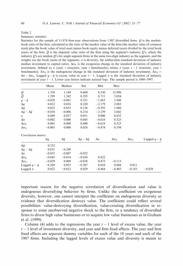
Table 2 shows summary statistics and cross-correlations for the sample ofdiversified firms. The sample contains 11,974 annual observations for 1,987 differentdiversified firms in the 18 year period of 1980–1997. The average number of segmentsper firm is 2.7. The number of firms per year declines over time, from a high of 872 in1981 to a low of 482 in 1997. Average and median excess values are negative at �2.8and �6.1%.2 Since the standard deviation of exogenous diversity change is 0.040 andthe standard deviation of total diversity change is 0.045, most (80%) of the variationin diversity change is due to exogenous industry shocks. A statistic that is not shownin Table 2 is the correlation of industry investment and industry Q: Across industry-years, the correlation is 0.332, a moderately high positive correlation.

4. Diversity in investment

Table 3 shows basic results for regressions of changes in excess value on changes indiversity in industry investment. The regression is simple pooled OLS; the standarderrors have been adjusted for correlation of the residuals within years, and forheteroskedasticity. The robust standard errors allow for clustered sampling(dependence of observations within each year), following Rogers (1993). The firstcolumn shows that the coefficient on the change in diversity is negative andsignificant. The coefficient implies that a one standard deviation increase in diversitylowers excess value by 1.1%.

One can use the coefficient on Ds to calculate the potential contribution ofdiversity in explaining the average level of the diversification discount. Mechanically,a focused firm has a s of zero. Since the mean of s is 0.049, the average level ofdiversity explains an average discount of �0:25*0:049 or 1.2%. Since the averagediscount in this sample is 2.8%, investment diversity alone can explain more than40% of the level of the average discount.

Column (2) shows the results using the exogenous change in diversity. Exogenouschanges in diversity have a negative and significant effect on excess value. Thisfinding is the major result of this paper: diversification is negatively correlated withvalue not just due to selection biases and endogenous choices by firms, but alsobecause higher levels of diversification somehow cause value destruction.

Column (3) shows that both exogenous and endogenous changes in diversity arenegatively related to changes in excess value. Thus, as often hypothesized, an

2In interpreting the values it is important to note that the natural logarithm is a concave function. Since

firm-level variables are more volatile than industry-level variables, average log ratios tend to be negative.

For example, mean Q is above mean %Q; but mean q � %q is negative. Looking at excess value without logs,

the mean of Q � %Q is 3.9% and the median is �6.8%.


important reason for the negative correlation of diversification and value isendogenous diversifying behavior by firms. Unlike the coefficient on exogenousdiversity, however, one cannot interpret the coefficient on endogenous diversity asevidence that diversification destroys value. The coefficient could reflect severalpossibilities: value-destroying diversification, value-creating diversification in re-sponse to some unobserved negative shock to the firm, or a tendency of diversifiedfirms to divest high value businesses or to acquire low value businesses as in Grahamet al. (1999).

Column (4) adds to the regressions the year t � 1 level of excess value, the yeart � 1 level of investment diversity, and year and firm fixed effects. The year and firmfixed effects are separate dummy variables for each of the 18 years and each of the1987 firms. Including the lagged levels of excess value and diversity is meant to

Table 2

Summary statistics

Statistics for the sample of 11,974 firm-year observations from 1,987 diversified firms. Q is the market-

book ratio of the firm, calculated as the ratio of the market value of the firm (the market value of common

stock plus the book value of total asset minus book equity minus deferred taxes) divided by the total book

assets of the firm. %Q is the imputed value ratio of the firm using the segment’s industry Q’s, where the

industry Q’s are median Q’s for single segment firms in the same two-digit industry as the segment, and the

weights are the book assets of the segments. s is diversity, the within-firm standard deviation of industry

median investment to capital ratios. DsX is the exogenous change in the standard deviation of industry

investment, defined as s (year t structure, year t benchmarks) minus s (year t � 1 structure, year t

benchmarks). DsN is the endogenous change in the standard deviation of industry investment, DsN ¼Ds� DsX: Lagged q � %q is excess value in year t � 1: Lagged s is the standard deviation of industry

investment in year t � 1: Lower case letters indicate natural logs. The sample period is 1980–1997.

Mean Median Std Min Max

Q 1.338 1.149 0.660 0.350 12.998%Q 1.299 1.242 0.293 0.711 5.054

q � %q �0.028 �0.061 0.351 �1.863 1.848

Dq 0.012 0.016 0.220 �2.179 2.083

D %q 0.022 0.032 0.126 �0.592 1.060

Dq � D %q �0.010 �0.006 0.214 �2.239 2.042

s 0.049 0.037 0.051 0.000 0.652

Ds �0.002 0.000 0.045 �0.618 0.525

DsX 0.001 0.000 0.040 �0.618 0.525

DsN �0.003 0.000 0.026 �0.474 0.194

Correlation matrix

Dq D %q Dq � D %q Ds DsX DsN Lagged q � %q

D %q 0.332

Dq � D %q 0.831 �0.249

Ds �0.055 �0.007 �0.052

DsX �0.043 �0.014 �0.036 0.822

DsN �0.029 0.009 �0.036 0.472 �0.113

Lagged q � %q �0.269 0.053 �0.307 0.010 0.004 0.011

Lagged s 0.022 �0.012 0.029 �0.464 �0.403 �0.185 �0.038


capture predictable mean reversion in these variables. The negative coefficient onlagged excess value reflects the fact that excess value tends to move towards its mean.Economically, this mean reversion can occur because firms with high excess valuesinvest more (so that their book value goes up and the ratio of market to book falls),or because they tend to have low subsequent returns (so their market value goesdown), as in Lamont and Polk (2001).

Including the lagged level of diversity helps to control for predictable movementsin diversity. As seen in Table 2, exogenous changes in diversity are quite predictableusing the lagged level of diversity, since the correlation between the two variables is�0.40. Expected changes in diversity (due to expected changes in industryconditions) should already be reflected in market values as of year t � 1: Since weare interested in examining the effects of industry shocks on value, we purge changesin diversity of their expected component by putting the lagged level of diversity intothe regression.

These additional control variables do not change the basic result that bothexogenous and endogenous changes in diversity are negatively related to firm value.The coefficient on exogenous changes rises somewhat, while the coefficient onendogenous diversity is little changed. We use column (4) as our baseline regression.

4.1. Effects of measurement error

Measurement error is an issue in Table 3 since both the dependent variable and theindependent variable are constructed using the same segment information and

Table 3

Basic regression of change in excess value on change in diversity

The dependent variable is Dq � D %q; the change in excess value. Ds is the change in the standard deviation

of industry investment. DsX is the exogenous change in the standard deviation of industry investment,

caused only by changes in industry characteristics. DsN is the endogenous change in the standard deviation

of industry investment, caused only by change in corporate structure including number and SIC code of

segments. Lagged q � %q is excess value in year t � 1: Lagged s is the standard deviation of industry

investment in year t � 1: The number of observations is 11,974; the sample period is 1980–1997. ‘‘Year and

firm dummies’’ indicate separate intercepts for each of 18 years and each of the 1987 firms. The standard

errors, in parentheses, are calculated allowing for both heteroskedasticity and for the residuals to be

correlated within each of the 18 years, 1980–1997.

(1) (2) (3) (4)

Ds �0.250 (0.052)

DsX �0.193 (0.066) �0.217 (0.062) �0.302 (0.069)

DsN �0.338 (0.120) �0.324 (0.124)

Lagged q � %q �0.470 (0.027)

Lagged s �0.197 (0.095)

Constant �0.010 (0.007) �0.010 (0.007) �0.010 (0.007)

R2 0.003 0.001 0.003 0.366

Year and firm dummies N N N Y


industry characteristics. If the segment information (such as SIC codes) or thecharacteristics are observed with error, this measurement error can lead to faultyinferences. In the case of industry characteristics, the most relevant source ofmeasurement error is probably inappropriate matching of focused firms withdiversified firm segments. Chevalier (1999) provides evidence supporting thisconclusion. If focused firms are fundamentally different from diversified firms, orif there is some noise in the process of matching focused firms to diversified firms,then industry characteristics will be noisy measures of firm value and of segmentcharacteristics.

Other sources of measurement error include Compustat coding errors, a majorissue in the segment database. Lamont (1997) examined segment data for 26 firmsbetween 1985 and 1987 and found coding errors in four (15%). Hyland (2000) foundexamined segment data for 243 firms between 1978 and 1992, and found codingerrors in 29 (12%), of which 16 involved backfilling of segment data.

The same measurement error appearing in both the dependent and independentvariables can lead to spurious results. In interpreting the regression coefficients incolumns (1) and (2) of Table 3, the following simple framework is helpful. Supposethe true relation is

Dq � D %qn ¼ aþ bDdn þ e; ð3Þ

where %qnis the true log imputed value ratio for the firm and dn is the true diversitymeasure. We observe noisy measures of the true variables

D %q ¼ D %qn þ u; ð4Þ

Dd ¼ Ddn þ v: ð5Þ

Since both D %q and Dd are constructed using the same underlying variables, in generalboth cov(D %qn; Ddn) and cov(v; u) will be non-zero. If one regresses is Dq � D %q on Dd;the estimated coefficient (assuming that the measurement errors, u and v; areuncorrelated with the disturbance term e) is

b ¼b varðDdnÞ � covðv; uÞ

varðDdnÞ þ varðvÞ¼ b

varðDdnÞvarðDdnÞ þ varðvÞ

�covðv; uÞ

varðDdnÞ þ varðvÞ: ð6Þ

Measurement error induces a biased coefficient in two ways. First, the familiarattenuation effect varðDdnÞ=ðvarðDdnÞ þ varðvÞÞ moves the coefficient towards zero.Second, the covariance term �covðv; uÞ=ðvarðDdnÞ þ varðvÞÞ causes b to be biasedeither positively or negatively. We call this second term ‘‘covariance bias’’, andconsider it separately from attenuation.

While we cannot directly observe the covariance bias, we can observe c ¼ððcovðv; uÞ þ covðD %qn;DdnÞÞÞ=ðvarðDdnÞ þ varðvÞÞ; which is the coefficient in aregression of D %q on Dd: With a further assumption about the measurement error,we can bound the covariance bias. Let r be the fraction of cov(D %q; Dd) that is due tomeasurement error, r ¼ covðv; uÞ=covðD %q;DdÞ: The covariance bias is then �rc: Anatural extreme value of r is one, which corresponds to a scenario in which thematching procedure is completely useless and measurement error is so large thateither the diversity measure or %q (or both) are complete noise. Although any value of


Table 4

Robustness to measurement error and outliers

In regressions (1)–(3), the dependent variable is D %q; the change in the natural log of %Q: %Q is the imputed value ratio, the weighted average of the segment’s

industry Q’s. Ds is the change in the standard deviation of industry investment ratios. DsX is the exogenous change in the standard deviation of industry

investment ratios, caused only by changes in industry characteristics. DsN is the endogenous change in the standard deviation of industry investment ratios,

caused only by change in corporate structure. Lagged q � %q is excess value in year t � 1: Lagged s is the standard deviation of industry investment in year t � 1:In regressions (4)–(6), the dependent variable is Dq � D %q; the change in excess value. ‘‘No outliers’’ discards observations of Dq � D %q; DsX; and DsN; that are in

the top or bottom 0.5% of their distributions. ‘‘Year and firm dummies’’ indicate separate intercepts for each year and firm. The number of observations is

11,974 (except for column (6), which is 11,624); the sample period is 1980–1997. The standard errors, in parentheses, are calculated allowing for both

heteroskedasticity and for the residuals to be correlated within each year.

D %q on left-hand side Dq � D %q on left-hand side

No outliers

(1) (2) (3) (4) (5) (6)

Ds �0.020 (0.117)

DsX �0.045 (0.146) 0.024 (0.107) �0.212 (0.072) �0.289 (0.071) �0.277 (0.095)

DsN �0.003 (0.065) �0.326 (0.103) �0.337 (0.056)

Lagged q � %q 0.049 (0.012) �0.444 (0.024) �0.399 (0.028)

Lagged s �0.139 (0.060) �0.272 (0.085) �0.239 (0.088)

D %q �0.423 (0.039) �0.535 (0.045)

Constant 0.022 (0.021) 0.022 (0.021) �0.000 (0.008)

R2 0.000 0.000 0.555 0.064 0.411 0.340

Year and firm dummies N N Y N Y Y

O.A

.L

am

on

t,C

.P

olk

/J

ou

rna

lo

fF

ina

ncia

lE

con

om

ics6

3(

20

02

)5

1–

77

63

r is possible, values between zero (corresponding to no measurement error) and one(corresponding to huge measurement error) seem most reasonable. We leave it to thereaders to choose r as they see fit.

Columns (1) and (2) in Table 4 show estimates of the coefficient c: Consider theregression in column (2) of Table 3, which shows a coefficient of �0.193 forexogenous changes in diversity. Column (2) of Table 4 shows that for this regression,c is �0.045. Thus if r is between zero and one, the true coefficient actually has ahigher magnitude than the estimated coefficient, as both attenuation bias andcovariance bias move the estimate towards zero. Thus measurement error cannotexplain the negative and significant coefficient in column (2) of Table 3.

Column (3) of Table 4 shows the multiple regression version with change in logimputed value as the dependent variable and our baseline variables on the right handside. The coefficient for exogenous diversification is now positive but low at 0.024.This positive coefficient with D %q as the dependent variable obviously tends toproduce a negative coefficient when Dq � D %q is the dependent variable. Compared tothe coefficient of �0.302 in column (4) of Table 3, however, the coefficient of 0.024seems basically irrelevant.

Columns (4) and (5) of Table 4 show the effect of adding D %q to the right-hand sideof the regressions. First, column (4) adds change in imputed value to the two-variable regression. Using the measurement error framework, in this regression thecovariance bias is positive if r is greater than 0.42.3 Despite a potentially positivebias when measurement error is extreme, exogenous changes in diversity still have anegative and significant effect. Including D %q in the baseline specification, in column(5), slightly lowers the coefficient on exogenous changes in diversity, but thecoefficient is still negative and significant.

The last column of Table 4 discards extreme observations, defined as anyobservation which is in the top 0.5% or bottom 0.5% of the distribution of Dq � D %q;DsN; and DsX: The coefficient on the exogenous changes in diversity is slightly lowerthan the baseline results, but is still negative and significant.

In summary, our results are very unlikely to be driven by measurement error. Aswe will see later, however, measurement error can be an important concern whenusing other measures of diversity in investment opportunities.

4.2. Alternative specifications

Table 5 explores the stability of our main results. Since our main interest is thecausal role of diversity, we focus on the coefficient on exogenous diversity change.

3Using the measurement error framework, the coefficient on exogenous change in diversity is

b varðDdnÞ þ covðD %qn; DdnÞ � covðDq; D %qÞcovðD %q;DdÞ=varðD %qÞ

varðDdnÞ þ varðvÞ � covðD %q;DdÞ½ �2=varðD %qÞ.The bottom of this fraction is positive. The sign of the covariance bias depends on the sign of

covðD %q; DdÞð1� rÞ � covðDq;D %qÞcovðD %q;DdÞ=varðD %qÞ: Plugging in numbers, the sign of the bias is

negative as long as r is less than 0.42.


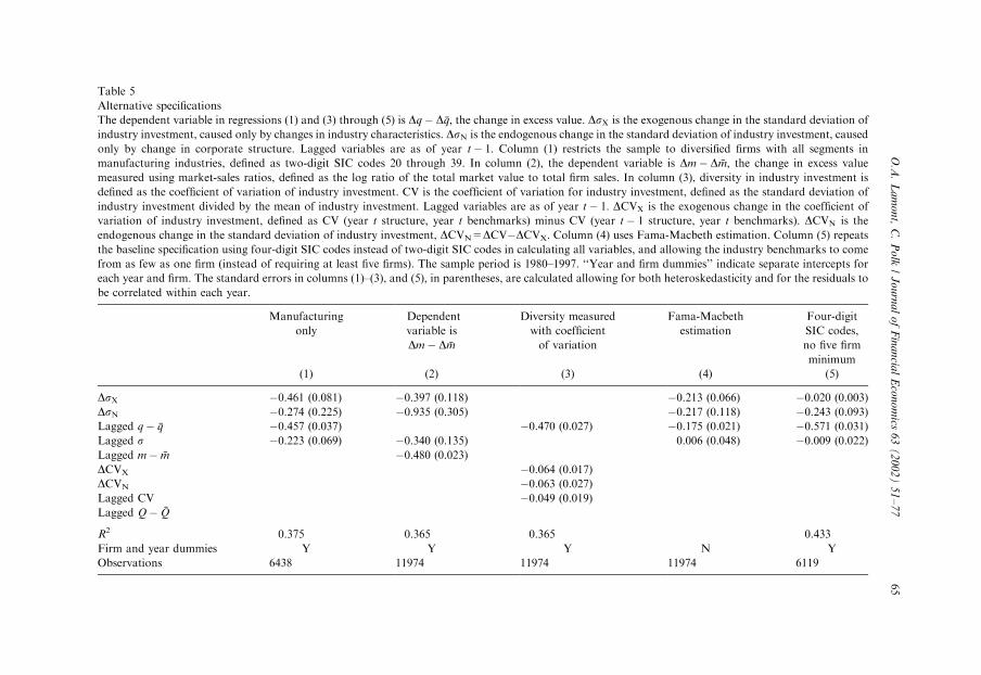
Table 5

Alternative specifications

The dependent variable in regressions (1) and (3) through (5) is Dq � D %q; the change in excess value. DsX is the exogenous change in the standard deviation of

industry investment, caused only by changes in industry characteristics. DsN is the endogenous change in the standard deviation of industry investment, caused

only by change in corporate structure. Lagged variables are as of year t � 1: Column (1) restricts the sample to diversified firms with all segments in

manufacturing industries, defined as two-digit SIC codes 20 through 39. In column (2), the dependent variable is Dm � D %m; the change in excess value

measured using market-sales ratios, defined as the log ratio of the total market value to total firm sales. In column (3), diversity in industry investment is

defined as the coefficient of variation of industry investment. CV is the coefficient of variation for industry investment, defined as the standard deviation of

industry investment divided by the mean of industry investment. Lagged variables are as of year t � 1: DCVX is the exogenous change in the coefficient of

variation of industry investment, defined as CV (year t structure, year t benchmarks) minus CV (year t � 1 structure, year t benchmarks). DCVN is the

endogenous change in the standard deviation of industry investment, DCVN=DCV�DCVX. Column (4) uses Fama-Macbeth estimation. Column (5) repeats

the baseline specification using four-digit SIC codes instead of two-digit SIC codes in calculating all variables, and allowing the industry benchmarks to come

from as few as one firm (instead of requiring at least five firms). The sample period is 1980–1997. ‘‘Year and firm dummies’’ indicate separate intercepts for

each year and firm. The standard errors in columns (1)–(3), and (5), in parentheses, are calculated allowing for both heteroskedasticity and for the residuals to

be correlated within each year.

Manufacturing

only

Dependent

variable is

Dm � D %m

Diversity measured

with coefficient

of variation

Fama-Macbeth

estimation

Four-digit

SIC codes,

no five firm

minimum

(1) (2) (3) (4) (5)

DsX �0.461 (0.081) �0.397 (0.118) �0.213 (0.066) �0.020 (0.003)

DsN �0.274 (0.225) �0.935 (0.305) �0.217 (0.118) �0.243 (0.093)

Lagged q � %q �0.457 (0.037) �0.470 (0.027) �0.175 (0.021) �0.571 (0.031)

Lagged s �0.223 (0.069) �0.340 (0.135) 0.006 (0.048) �0.009 (0.022)

Lagged m � %m �0.480 (0.023)

DCVX �0.064 (0.017)

DCVN �0.063 (0.027)

Lagged CV �0.049 (0.019)

Lagged Q � %Q

R2 0.375 0.365 0.365 0.433

Firm and year dummies Y Y Y N Y

Observations 6438 11974 11974 11974 6119

O.A

.L

am

on

t,C

.P

olk

/J

ou

rna

lo

fF

ina

ncia

lE

con

om

ics6

3(

20

02

)5

1–

77

65

Column (1) shows the results of discarding diversified firms that have anysegments in nonmanufacturing industries. One might expect measurement error indiversity to be lower in this regression, since investment to capital ratios are less well-behaved in nonmanufacturing industries such as services, mining, and agriculture.Column (1), which has a sample size of about half the baseline sample, shows thecoefficient on exogenous change in diversity becomes more negative and remainssignificant.

Column (2) shows a version of the baseline regression replacing Q everywhere withM ; the ratio of the market value to the total sales of the firm. The relation betweenexcess value and exogenous diversity is again stronger compared to the baselineresults. The coefficient on endogenous diversity is much higher but is estimatedimprecisely. Column (3) measures diversity using the coefficient of variation ofindustry investment (the ratio of standard deviation to mean), rather than thestandard deviation of industry investment. Again, the exogenous change in diversityhas a significant negative effect (the coefficient is different from the baselineregression because the units of the diversity change variable are different). Column(4) uses Fama-Macbeth estimation; the coefficients on the exogenous change indiversity remain negative and significant.

Column (5) shows the effects of redoing the analysis using industry benchmarks(for both excess value and diversity) based on the four-digit SIC code of theindividual segment, instead of two-digit SIC codes used elsewhere. Unfortunately,this increase in precision comes at the cost of reducing the number of observations,since it is more difficult to find five matching four-digit firms for each segment ofthe firm. To maintain a large sample size, we relax the constraint of a minimumof at least five matching focused firms, and instead require a minimum of onlyone matching firm. In other words, we allow the industry benchmark to consistof a single firm or the median of multiple firms. Thus the benchmarks underlyingcolumn (5) have better matching by industry, but also have greater noise due tofirm-specific random variation. As a result, the diversity change variable has amuch greater variance, presumably due to greater measurement error. Despitethis noise, the coefficient on exogenous diversity change is still negative andsignificant.

In summary, our results are robust to alternate specifications, and are especiallystrong for manufacturing firms. This robustness to alternate specifications furthersuggests that measurement error or misspecification is not the driving factor.

4.3. Alternate measures of diversity in investment

Here we explore two alternate measures of investment diversity that incorporateinformation about the relative size of the various segments. The first measure weexamine is diversity in resource-weighted investment. Rajan et al. (2000) present atheory in which both the diversity in segment resources and in segment investmentopportunities determines investment allocation. They use a measure involving thestandard deviation of investment opportunities multiplied by relative segment size(we examine their specific measure in the next section).


Our analog is the standard deviation of weighted investment, s1:

s1 ¼

ffiffiffiffiffiffiffiffiffiffiffiffiffiffiffiffiffiffiffiffiffiffiffiffiffiffiffiffiffiffiffiffiffiffiffiffiffiffiffiffiffiffiffiffiffiffiffiffiffiffiffiffiffiffiffiffiffiffiffiffiffiffiffiffiffiffiffiffiffiffiffiffiffiffiffiffiffiffiffiffiffiffiffiffiffiffiffiffiffiffiffiffiffi1

n � 1

Xn

j¼1wjIIND j �

1

n

Xn

i¼1wiIIND i

� � 2

;

sð7Þ

where again wj is the fraction of the firm’s assets in segment j; IINDj is industryinvestment for segment j; and the firm has n segments. s1 is diversity in asset-weighted investment. According to s1; a firm can have high diversity even if industryinvestment is the same for each segment, as long as it has segments of different size.

Table 6

Alternative measures of investment diversity

The dependent variable is Dq � D %q; the change in excess value. s1 is the standard deviation of asset-

weighted industry investment. s2 is the weighted standard deviation of industry investment.

s1 ¼

ffiffiffiffiffiffiffiffiffiffiffiffiffiffiffiffiffiffiffiffiffiffiffiffiffiffiffiffiffiffiffiffiffiffiffiffiffiffiffiffiffiffiffiffiffiffiffiffiffiffiffiffiffiffiffiffiffiffiffiffiffiffiffiffiffiffiffiffiffiffiffiffiffiffiffiffiffiffiffiffiffiffiffiffiffiffiffiffiffiffiffiffi1

n � 1

Xn

j¼1wjIIND j �

1

n

Xn

i¼1wiIIND i

� � 2s

and

s2 ¼

ffiffiffiffiffiffiffiffiffiffiffiffiffiffiffiffiffiffiffiffiffiffiffiffiffiffiffiffiffiffiffiffiffiffiffiffiffiffiffiffiffiffiffiffiffiffiffiffiffiffiffiffiffiffiffiffiffiffiffiffiffiffiffiffiffiffiffiffiffiffiffiffiffiffiffiffiffiffiffiffiffiffiffiffiffiffiffiffin

n � 1

Xn

j¼1wj IIND j �

Xn

i¼1wiIIND i

h i� �2r

where wj is the fraction of the firm’s assets in segment j; IINDj is industry investment for segment j; and the

firm has n segments. Ds1X is the exogenous change in the standard deviation of asset-weighted industry

investment and Ds1N is the endogenous change. Ds2X is the exogenous change in the weighted standard

deviation of industry investment and Ds2N is the endogenous change. DsX is the exogenous change in the

standard deviation of industry investment and DsN is the endogenous change. Lagged variables are as of

year t � 1: The number of observations is 11,974. All regressions include separate intercepts for each year

and firm. The standard errors, in parentheses, are calculated allowing for both heteroskedasticity and for

the residuals to be correlated within each year.

(1) (2) (3) (4)

Ds1X �0.439 (0.168) �0.377 (0.163)

Ds1N �0.102 (0.066) �0.019 (0.062)

Ds2X �0.348 (0.085) �0.140 (0.219)

Ds2N �0.461 (0.164) �0.508 (0.300)

DsX �0.258 (0.067) �0.194 (0.166)

DsN �0.332 (0.127) 0.040 (0.209)

Lagged q � %q �0.471 (0.028) �0.472 (0.027) �0.470 (0.027) �0.470 (0.027)

Lagged s1 �0.244 (0.080) �0.218 (0.077)

Lagged s2 �0.195 (0.105) 0.139 (0.290)

Lagged s �0.174 (0.095) �0.311 (0.261)

Joint significance of

both exogenous

changes (p-value)

0.000 0.000

R2 0.366 0.368 0.366 0.367


Our second alternate measure of investment diversity takes the opposite approachwith segment size. The weighted standard deviation is s2:

s2 ¼

ffiffiffiffiffiffiffiffiffiffiffiffiffiffiffiffiffiffiffiffiffiffiffiffiffiffiffiffiffiffiffiffiffiffiffiffiffiffiffiffiffiffiffiffiffiffiffiffiffiffiffiffiffiffiffiffiffiffiffiffiffiffiffiffiffiffiffiffiffiffiffiffiffiffiffiffiffiffiffiffiffiffiffiffiffiffiffin

n � 1

Xn

j¼1wj IIND j �

Xn

i¼1wiIIND i

h i� �2r

: ð8Þ

In calculating diversity, s2 gives more weight to bigger segments. Consider a firmwith 99% of its assets in one segment and 1% of its assets in another segment.Ceteris paribus, while s1 would view this firm as extremely diverse, s2 would viewthis firm as not at all diverse and almost the same as a focused firm.

Table 6 shows results for the effect of diversity on excess value, again decomposingthe change in diversity into an exogenous component reflecting changes in industryinvestment and an endogenous component reflecting changes in structure (whichnow include changes in segment assets). We show the diversity measures bythemselves, and then in conjunction with our baseline diversity measure. As before,we include the lagged level of the particular diversity measure.

Column (1) shows the regression using s1; diversity in asset-weighted investment.As with the baseline specification, exogenous changes in diversity have a negativeand significant effect on excess value. Column (2) adds changes in baseline diversity.The coefficient on DsX is slightly lower than the coefficient in the baselinespecification, and the coefficient on Ds1X falls somewhat. Both exogenous changesare individually significant. Measurement error does not appear to be a problem incolumn (2), as the regression (not shown) of D %q on column (2)’s right-hand sidevariables results in a coefficient of 0.14 on Ds1X and �0.01 on DsX: Thus there isevidence that exogenous changes in asset-weighted diversity (in addition tounweighted diversity) destroy firm value. We interpret this surprising result as avictory for the resource-weighted approach Rajan et al. (2000) advocate.

Column (3) shows the results using s2; the weighted standard deviation ofinvestment. The coefficients are similar to the baseline specification. Column (4)shows the effect of adding s: It turns out that DsX and Ds2X have a correlation of0.95, so that multicollinearity plagues column (4). Although neither DsX nor Ds2X

are individually significant, they are strongly significant jointly. Thus we concludefrom columns (3) and (4) that it is impossible to tell whether DsX and Ds2X haveseparate effects on value, and that it does not much matter whether one uses thesimple standard deviation or the weighted standard deviation in measuringinvestment diversity.

4.4. Direct measures of firm investment diversity

The evidence so far is consistent with the inefficient internal capital marketshypothesis. Here we provide more direct evidence using actual investment at thesegment level, instead of just industry investment. Although this evidence cannotshow causality, it also supports the hypothesis. Consistent with the results ofScharfstein (1998), Gertner et al. (1999), and others, we find that diversified firmsallocate capital expenditures in a socialistic manner.


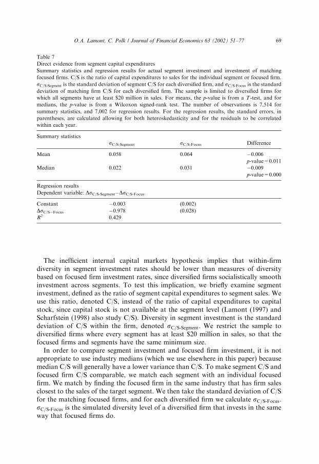
The inefficient internal capital markets hypothesis implies that within-firmdiversity in segment investment rates should be lower than measures of diversitybased on focused firm investment rates, since diversified firms socialistically smoothinvestment across segments. To test this implication, we briefly examine segmentinvestment, defined as the ratio of segment capital expenditures to segment sales. Weuse this ratio, denoted C/S, instead of the ratio of capital expenditures to capitalstock, since capital stock is not available at the segment level (Lamont (1997) andScharfstein (1998) also study C/S). Diversity in segment investment is the standarddeviation of C/S within the firm, denoted sC=S-Segment: We restrict the sample todiversified firms where every segment has at least $20 million in sales, so that thefocused firms and segments have the same minimum size.

In order to compare segment investment and focused firm investment, it is notappropriate to use industry medians (which we use elsewhere in this paper) becausemedian C/S will generally have a lower variance than C/S. To make segment C/S andfocused firm C/S comparable, we match each segment with an individual focusedfirm. We match by finding the focused firm in the same industry that has firm salesclosest to the sales of the target segment. We then take the standard deviation of C/Sfor the matching focused firms, and for each diversified firm we calculate sC=S-Focus:sC=S-Focus is the simulated diversity level of a diversified firm that invests in the sameway that focused firms do.

Table 7

Direct evidence from segment capital expenditures

Summary statistics and regression results for actual segment investment and investment of matching

focused firms. C/S is the ratio of capital expenditures to sales for the individual segment or focused firm.

sC=S-Segment is the standard deviation of segment C/S for each diversified firm, and sC=S-Focus is the standard

deviation of matching firm C/S for each diversified firm. The sample is limited to diversified firms for

which all segments have at least $20 million in sales. For means, the p-value is from a T-test, and for

medians, the p-value is from a Wilcoxon signed-rank test. The number of observations is 7,514 for

summary statistics, and 7,002 for regression results. For the regression results, the standard errors, in

parentheses, are calculated allowing for both heteroskedasticity and for the residuals to be correlated

within each year.

Summary statistics

sC/S-Segment sC/S-Focus Difference

Mean 0.058 0.064 �0.006

p-value=0.011

Median 0.022 0.031 �0.009

p-value=0.000

Regression results

Dependent variable: DsC/S-Segment�DsC/S-Focus

Constant �0.003 (0.002)

DsC/S�Focus �0.978 (0.028)

R2 0.429


Table 7 shows summary statistics for the diversity of segment investment. Aspredicted by the inefficient internal capital markets hypothesis, actual segmentinvestment is smoother than the investment of focused firms in the same industry.Although the two measures of diversity are positively correlated (the correlation is0.197), both mean and median sC=S-Focus are significantly higher than sC=S-Segment:

Another implication of the inefficient internal capital markets hypothesis is thatsC=S-Segment should not move one-for-one with sC=S-Focus: This implication is centralto our tests using exogenous changes in diversity, as excess values increase whendiversity decreases due to shocks to industry benchmarks. In Table 7, we reportevidence from segment investment supporting this implication. We test whether thedifference in sC=S-Focus and sC=S-Segment fluctuates when sC=S-Focus fluctuates. IfDsC=S-Segment is uncorrelated with DsC=S-Focus; then a regression of DsC=S-Segment �DsC=S-Focus on DsC=S-Focus should result in a coefficient of negative one. Table 7 showsthat the coefficient is not significantly different from negative one. However, we notethat measurement error (along the lines discussed previously) is a major concern in

Table 8

Diversity in asset-weighted Q

The dependent variable is DQ � D %Q: RSZ is diversity in asset-weighted Q; defined as the standard

deviation of asset-weighted Q; divided by %QEW ¼ ð1=nÞP

j QIND j ; the equal-weighted average of QIND J.

RSZ ¼1

%QEW

ffiffiffiffiffiffiffiffiffiffiffiffiffiffiffiffiffiffiffiffiffiffiffiffiffiffiffiffiffiffiffiffiffiffiffiffiffiffiffiffiffiffiffiffiffiffiffiffiffiffiffiffiffiffiffiffiffiffiffiffiffiffiffiffiffiffiffiffiffiffiffiffiffiffiffiffiffiffiffiffiffiffiffiffiffiffiPnj¼1 wjQIND j � ð1=nÞ

Pni¼1 wiQIND i

� �� 2n � 1

;

s

where wj is the fraction of the firm’s assets in segment J; and QIND J is the benchmark Q for segment J’s

industry. DRSZX is the exogenous change in RSZ, caused only by changes in industry characteristics.

DRSZN is the endogenous change in RSZ, caused only by change in corporate structure including number

and SIC code of segments and weights. Dln(Sales) is the log change in total firm sales. DsX is the

exogenous change in the standard deviation of industry investment ratios, caused only by changes in

industry characteristics. DsN is the endogenous change in the standard deviation of industry investment

ratios, caused only by change in corporate structure. The number of observations is 11,974. All regressions

include separate intercepts for each year and firm. The standard errors, in parentheses, are calculated

allowing for both heteroskedasticity and for the residuals to be correlated within each year.

DQ � D %Q on left-hand side D %Q on left-hand side

(1) (2) (3) (4) (5)

DRSZ �0.116 (0.047)

DRSZX �0.664 (0.156) �0.459 (0.138) 0.906 (0.127) 1.290 (0.064)

DRSZN �0.076 (0.052) 0.036 (0.010)

D1= %QEW 0.947 (0.140) 0.985 (0.147) �1.667 (0.080)

Dln(Sales) �0.082 (0.044) �0.084 (0.044) 0.003 (0.007)

Constant �0.015 (0.012) 0.028 (0.028)

R2 0.223 0.225 0.001 0.030 0.861

Firm and year

dummies

Y Y N N Y


this regression. Random noise in individual firm investment tends to drive thecoefficient towards negative one.

In addition to the problem of measurement error, Table 7 suffers from selectionbiases, since it examines endogenously chosen investment levels. Nevertheless, it atleast shows that the available evidence on segment investment is consistent with thehypothesis that capital expenditures are inefficiently allocated within the firm. Takentogether with the evidence shown previously on the causal channel betweeninvestment diversity and excess value, Table 7 provides direct evidence on how thiscausal channel operates. It appears that at least part of the value destruction weshow occurs because internal capital markets are inefficient.

5. Diversity of different characteristics

Table 8 examines the diversity measure of Rajan et al. (2000), which we call RSZ.RSZ is the diversity in asset-weighted Q; and is defined as:

RSZ ¼stdev wjQIND j

� �%QEW

¼

ffiffiffiffiffiffiffiffiffiffiffiffiffiffiffiffiffiffiffiffiffiffiffiffiffiffiffiffiffiffiffiffiffiffiffiffiffiffiffiffiffiffiffiffiffiffiffiffiffiffiffiffiffiffiffiffiffiffiffiffiffiffiffiffiffiffiffiffiffiffiffiffiffiffiffiffiffiffiffiffiffiffiffiffiPnj¼1 wjQIND j � ð1=nÞ

Pni¼1 wiQIND i

� �� 2n � 1

s

ð1=nÞP

j QIND j

ð9Þ

%QEW is equal-weighted industry Q: As in our measure s1; the RSZ measure involvesdiversity in segment size measured by book assets.

Column (1) of Table 8 reproduces basic results on excess value using a first-differenced version of the specification in Rajan et al. (2000). In addition to themeasure of diversity, their specification also includes the log of firm size and theinverse of the equal-weighted Q across the segments. The dependent variable is thefirst difference in excess value, measured without logs. The regression is not exactlythe same as theirs because Rajan et al. (2000) use levels instead of differences, have ashorter time period, match by three digit SIC codes instead of two, use a morecomplex measure of Tobin’s Q rather than the market-book ratio, and Winsorize thevariables. Nevertheless, the results are broadly similar, as the coefficient of �0.116(with t-statistic of 2.5) on diversity corresponds to the estimate of �0.276 (with t-statistic of 5.7) in Rajan, Servaes, and Zingales.

Column (2) splits the change in RSZ into exogenous and endogenous components,where as before the endogenous change reflects changes in corporate structure andthe exogenous change reflects changes in industry characteristics. Column (2) showsthat the effect of diversity comes largely through exogenous changes in diversity, asthe coefficient on the exogenous change in RSZ is large and significant. Thus column(2) shows that endogeneity is not a major concern for the Rajan et al. (2000) results.4

4 In the working paper version, Rajan et al. (1998) perform a robustness test that is somewhat similar to

our exogenous/endogenous distinction. They show that their results survive after dropping firms for which

individual segments experience large changes in asset value. They also control for the number of segments.

However, these robustness tests are performed for a regression examining segment investment, not for a

regression involving excess value.


The major concern in Table 8 is measurement error, since industry Q’s now enterdirectly into the diversity measure as well as the dependent variable. Thusmeasurement error in industry Q’s has a greater potential to produce spuriousresults. To gauge the effects of measurement error, we start by putting the exogenouschange in RSZ diversity into a two-variable regression. Column (3) shows thecoefficient is still large and significant at �0.459. Column (4), however, shows thecoefficient c is 0.906 in this setting. Thus with a r of 0.51, measurement error cancompletely explain the estimated coefficient on exogenous change in RSZ. Of coursethe value of r is a judgement call that the reader must make. Readers who believemeasurement error is not a problem should set r ¼ 0; conservative readers who wantto avoid false inferences should set r higher.

The full specification Rajan et al. (2000) use includes as a control variable theinverse of average industry Q for the firm’s segments. Column (5) shows that thiscontrol variable does not eliminate the covariance bias. In the analogous multipleregression with the change in %Q as the dependent variable, the coefficient of 1.290 incolumn (5) is large, and could easily account for the coefficient of �0.664 in column(2).

Thus Table 8 shows that one must be careful in interpreting the empirical resultsusing the RSZ measure of diversity, since the results are quite sensitive toassumptions about measurement error. ‘‘Hard-wiring’’ in the construction of theindependent and dependent variables can lead to spurious results. Rajan et al. (2000)present a variety of evidence that measurement error is not driving their results,although most of their robustness tests involve other regressions with differentdependent and independent variables (since explaining excess value with diversity isnot their main focus). For these other regressions, they perform simulations,experiment with different control variables, and try alternative ways of constructingthe variables. Based on Table 8, we conclude that the Rajan, Servaes, and Zingalesresults on the relation between excess value and diversity are not convincing evidencein favor of their hypothesis, but this conclusion is a matter of opinion.

Despite these measurement error issues, we view our basic result, that diversitylowers firm value, as supporting the central premise of Rajan et al. (2000). And, asshown in Table 6, there is evidence that resource-weighting, as advocated by Rajan,Servaes, and Zingales, helps explain this value destruction.

5.1. Diversity in other characteristics

Berger and Ofek’s (1995) finding that excess values are lower for firms in unrelatedbusinesses is consistent with the inefficient internal capital markets hypothesis, but isalso consistent with the general notion that unrelated diversification is valuedestroying. Unrelated diversification could be bad due to greater scope for inefficientcross-subsidization, but it could also be bad for other reasons, such as limitedmanagerial talent. Since different industries have different levels of investment,diversity in industry investment could be proxying for more general diversity.Broadly, each year we would expect different industries to be different along manymeasurable dimensions, such as profitability, capital structure, and sales growth. The


Table 9

Diversity in leverage, cash flow, and sales growth

The dependent variable is Dq � D %q; the change in excess value. Leverage is the book value of debt divided by the sum of market value of equity and the book

value of debt. Sales growth is net sales in year t divided by net sales in year t � 1: Cash flow is income before extraordinary items plus depreciation in year t

divided by capital stock in year t � 1: DsX is the exogenous change in the standard deviation of industry investment ratios, caused only by changes in industry

characteristics. DsN is the endogenous change in the standard deviation of industry investment ratios, caused only by change in corporate structure. DsZX is

the exogenous change in the standard deviation of industry variable Z; caused only by changes in industry characteristics. DsZN is the endogenous change in

the standard deviation of industry variable Z; caused only by change in corporate structure. Lagged variables are as of year t � 1: All regressions include

separate intercepts for each year and firm. The number of observations is 11,974; the sample period is 1980–1997. The standard errors, in parentheses, are

calculated allowing for both heteroskedasticity and for the residuals to be correlated within each year.

Leverage: Z ¼Dt

Et þ Dt

Sales growth: Z ¼St

St�1Cash flow: Z ¼

CFt

Kt�1

DsZX �0.122 (0.081) �0.095 (0.085) �0.015 (0.101) 0.086 (0.112) �0.151 (0.043) �0.126 (0.040)

DsZN �0.264 (0.070) �0.184 (0.081) �0.447 (0.126) �0.263 (0.145) �0.241 (0.051) �0.229 (0.064)

DsX �0.251 (0.076) �0.296 (0.082) �0.210 (0.069)

DsN �0.187 (0.143) �0.210 (0.154) �0.045 (0.139)

Lagged q � %q �0.470 (0.028) �0.471 (0.027) �0.469 (0.028) �0.470 (0.027) �0.470 (0.028) �0.470 (0.027)

Lagged sZ �0.183 (0.034) �0.132 (0.040) �0.209 (0.114) �0.097 (0.124) �0.161 (0.038) �0.145 (0.038)

Lagged s �0.130 (0.100) �0.153 (0.099) �0.053 (0.094)

Joint significance of

DsZX and DsZN (p-value)

0.000 0.074 0.002 0.136 0.000 0.000

R2 0.366 0.367 0.365 0.367 0.367 0.368

O.A

.L

am

on

t,C

.P

olk

/J

ou

rna

lo

fF

ina

ncia

lE

con

om

ics6

3(

20

02

)5

1–

77

73

greater the diversity in these values in a given year, the greater the degree ofunrelated diversification.

Table 9 examines diversity in characteristics other than investment. For eachcharacteristic, we express diversity as the standard deviation in the industrycharacteristic. Table 9 examines each characteristic by itself and then in combinationwith investment diversity.

The first variable is leverage, the ratio of book debt to the sum of book debt andmarket equity. Lang et al. (1996) show that firm leverage is negatively related tocapital expenditures of noncore segments, suggesting that high leverage preventssegments from taking advantage of investment opportunities, and that combiningsegments with high optimal leverage and low optimal leverage results in valuedestruction. Table 9 shows that by itself, endogenous changes in leverage diversityare negatively related to firm value. There is no evidence that leverage diversitycauses lower values, since the exogenous change in leverage has a near zero effect.Finally, when adding the leverage diversity variables to our baseline regression, thecoefficient on exogenous changes in investment diversity remains negative andsignificant.

This pattern is repeated for diversity in sales growth, where sales growth is year t

net sales divided by year t � 1 net sales. Without investment diversity, onlyendogenous sales growth diversity has a negative and significant coefficient, and withinvestment diversity, both types of sales growth diversity are insignificant.

Cash flow diversity, however, does have a strong negative effect. Cash flow is theratio of income before extraordinary items to prior year capital stock. Withoutinvestment diversity, both endogenous and exogenous changes in cash flow diversityhave negative and significant coefficients. With investment diversity, the cash flowdiversity coefficients are little changed. Compared to the baseline results, thecoefficient on the exogenous change in investment diversity is somewhat lower at�0.210 instead of �0.302, and the coefficient on endogenous diversity changes fallsdramatically. Exogenous investment diversity changes still have a significant effect,therefore cash flow diversity does not subsume exogenous investment diversity.

How should one interpret the results on cash flow diversity and investmentdiversity? Berger and Ofek (1995) use the presence of a segment with negative cashflow (where the cash flow being used is actual segment cash flow, not industry cashflow) as a marker for cross-subsidization. In this sense, low segment cash flow issimilar to low segment investment opportunities in that it indicates a potential fordraining resources from the good segments to spend on the bad segments. Thus oneinterpretation of the negative effect of cash flow diversity is that it supports theinefficient internal capital markets hypothesis, since cash flow diversity creates asituation where good segments can subsidize bad segments. When the bad segmentsget worse and the good segments get better, the cross-subsidization problem becomesmore severe.

In summary, other measures of diversity do not subsume investment diversity.Cash flow diversity has an independent exogenous effect, however, which could beconsistent with the inefficient internal capital markets hypothesis, but could alsoreflect the more general idea that unrelatedness is bad.


6. Conclusions

Diversification destroys value. Our results show that exogenous increases in thediversity of a firm’s investment opportunities reduce firm relative value. Since welook at exogenous changes due to industry shocks, our results show that selectionbiases and endogenous diversifying behavior are not entirely responsible for theobserved diversification discount. We also study the effect of measurement error,and find that although measurement error can cause spurious results for somespecifications, our specification is relatively immune. These results support theinefficient internal capital markets hypothesis: diversified firms have low valuebecause they allocate capital inefficiently across their different parts.

Our analysis has limitations. It does not imply that if one randomly aggregatedfocused firms into diversified firms, value would be destroyed. What we show is thatexogenous increases in diversity destroy value, conditional on already beingdiversified.

We find that when firms endogenously choose to become more diversified, theirexcess value declines as well. In this case, however, the negative correlation betweenendogenous diversification and value may or may not be causal. Firms may bedestroying value by diversifying or firms may be diversifying in response to valuedecreases.

Our paper is similar in spirit to using natural experiments to identify causalityrather than correlation. Natural experiments, defined as episodes with large iden-tifiable economic shocks that are plausibly outside of the control of the firm, are hardto find. When one does find an experiment, sample sizes are often low (Blanchardet al. (1994) have 11 firms, while Lamont (1997) has 26). In contrast, our paperprovides a general technique to isolate causation in a wide variety of circumstances.

Future research could use this exogenous instrument in several ways. For example,Scharfstein (1998) and Palia (1999) find that diversified firms with higher CEO pay-for-performance sensitivity have higher values and appear to engage in lessinefficient cross-subsidization. Denis et al. (1997) find that the level of firmdiversification is negatively related to equity ownership of managers and outsideblockholders. One could test whether these results hold true for shocks to diversity:do exogenous shocks to diversity have a less negative effect in firms with betterincentives? If so, the results would support an agency explanation.

Appendix

Our data on segments comes from several Current and Research segment filesobtained from Wharton Research Data Services in April 1999. Our firm-levelCompustat and Center for Research in Securities Prices (CRSP) data comes from theUniversity of Chicago’s database in December 1999. In our calculation of marketvalue, we use CRSP market equity. For firms with multiple classes of stock, incalculating market equity, we aggregate all separate classes of stock together into onevalue-weighted portfolio.


We define Q as {market capitalization (from CRSP)+book assets (data item6)�book equity (data item 60)�deferred taxes (data item 74)}/book assets (data item6). The investment to capital ratio is capital expenditures (data item 128) divided byprior year net stock of property, plant, and equipment (data item 8). The market-sales ratio, M ; is (total debt+market capitalization)/net sales (data item 12).Leverage is total debt/(total debt+market capitalization) where total debt is definedas long-term debt (data item 9)+debt in current liabilities (data item 34)+redemp-tion value of preferred stock (data item 56). The cash flow is the sum of incomebefore extraordinary items (data item 18) and depreciation and amortization (dataitem 14), divided by prior year net stock of property, plant, and equipment (dataitem 8).

We drop firm-years if any of the following conditions hold: it has missing ornonpositive firm sales or firm assets; missing or nonpositive (for any segment)segment sales or segment assets; has any segment that Compustat assigns an one-digit SIC code of zero, six (financial), or nine (largely ‘‘NO OPERATIONS’’); thesum of segment sales is not within 1% of the total sales of the firm; the firm changesthe month of its fiscal year-end such that in December of year t � 1 our latestinformation is from year t � 2: We also drop firms (such as GM) who report multiplefirm totals for the same year (firms which report different Compustat total sales forthe same CRSP permanent company identifier number).

References

Berger, P., Ofek, E., 1995. Diversification’s effect on firm value. Journal of Financial Economics 37, 39–66.

Berger, P., Ofek, E., 1996. Bust-up takeovers of value-destroying diversified firms. Journal of Finance 51,

1175–1200.

Berger, P., Ofek, E., 1999. Causes and consequences of corporate refocusing programs. Review of

Financial Studies 12, 311–345.

Blanchard, O., Lopez-de-Silanes, F., Shleifer, A., 1994. What do firms do with cash windfalls? Journal of

Financial Economics 36, 337–360.

Campa, J., Kedia, S., 1999. Explaining the diversification discount. Unpublished working paper, New

York University, NY.

Chevalier, J., 1999. Why do firms undertake diversifying mergers? An examination of the investment

policies of merging firms. Unpublished working paper, University of Chicago.

Comment, R., Jarrell, G., 1995. Corporate focus and stock returns. Journal of Financial Economics 37,

67–87.

Daley, L., Mehrotra, V., Sivakumar, R., 1997. Corporate focus and value creation – evidence from

spinoffs. Journal of Financial Economics 45, 257–281.

Denis, D., Denis, D., Sarin, A., 1997. Agency problems, equity ownership, and corporate diversification.

Journal of Finance 52, 135–160.

Fluck, Z., Lynch, A., 1999. Why do firms merge and then divest? A theory of financial synergy. Journal of

Business 72, 319–346.

Fulghieri, P., Hodrick, L., 1997. Synergies and internal agency conflicts: the double-edged sword of

mergers. Unpublished working paper, Columbia University, NY.

Gertner, R., Powers, E., Scharfstein, D., 1999. Learning about internal capital markets from corporate

spinoffs. Unpublished working paper, University of Chicago, IL.

Graham, J., Lemmon, M., Wolf, J., 1999. Does corporate diversification destroy value? Unpublished

working paper, Duke University, NC.


Hadlock, C., Ryngaert, M., Thomas, S., 1999. Corporate structure and equity offerings: are there benefits

to diversification? Unpublished working paper, Michigan State University, Michigan.

Hubbard, R.G.H., Palia, D., 1999. A reexamination of the conglomerate merger wave in the 1960s: an

internal capital markets view. Journal of Finance 54, 1131–1152.

Hyland, D., 2000. Why firms diversify: an empirical examination. Unpublished working paper, University

of Texas, Arlington, TX.

John, K., Ofek, E., 1995. Asset sales and increase in focus. Journal of Financial Economics 37, 105–126.

Kaplan, S., Weisbach, M., 1992. The success of acquisitions: evidence from divestitures. Journal of

Finance 47, 108–138.

Lamont, O., 1997. Cash flow and investment: evidence from internal capital markets. Journal of Finance

52, 83–109.

Lamont, O., Polk, C., 2001. The diversification discount: cash flows vs. returns. Journal of Finance 56,

1693–1701.

Lang, L., Stulz, R., 1994. Tobin’s Q, corporate diversification, and firm performance. Journal of Political

Economy 102, 1248–1280.

Lang, L., Ofek, E., Stulz, R., 1996. Leverage, investment, and firm growth. Journal of Financial

Economics 40, 3–30.

Lewellen, W., 1971. A pure financial rationale for the conglomerate merger. Journal of Finance 26,

521–537.

Maksimovic, V., Phillips, G., 1999. Do conglomerate firms allocate resources inefficiently? Unpublished

working paper, University of Maryland.

Maquiera, C., Megginson, W., Nail, L., 1998. Wealth creation versus wealth re-distributions in pure stock-

for-stock mergers. Journal of Financial Economics 48, 3–33.

Morck, R., Shleifer, A., Vishny, R., 1990. Do managerial objectives drive bad acquisitions? Journal of

Finance 45, 31–48.

Palia, D., 1999. Corporate governance and the diversification discount: evidence from panel data.

Unpublished working paper, Columbia University, NY.

Peyer, U., Shivdasani, A., 2000. Leverage and internal capital markets: evidence from leveraged

recapitalizations. Journal of Financial Economics 59, 477–515.

Rajan, R., Servaes, H., Zingales, L., 1998. The cost of diversity: diversification discount and inefficient

investment. NBER working paper 6368.

Rajan, R., Servaes, H., Zingales, L., 2000. The cost of diversity: diversification discount and inefficient

investment. Journal of Finance 55, 35–80.

Rogers, W., 1993. Regression standard errors in clustered samples. Stata Technical Bulletin 13, 19–23.

Scharfstein, D., 1998. The dark side of internal capital markets II. NBER working paper 6352.

Scharfstein, D., Stein, J., 2000. The dark side of internal capital markets: divisional rent-seeking and

inefficient investment. Journal of Finance 55, 2537–2564.

Schlingemann, F., Stulz, R., Walkling, R., 1999. Corporate focusing and internal capital markets. NBER

working paper 7175.

Schoar, A., 1999. Effects of corporate diversification on productivity. Unpublished working paper,

Massachusetts Institute of Technology.

Servaes, H., 1996. The value of diversification during the conglomerate merger wave. Journal of Finance

51, 1201–1225.

Shin, H., Stulz, R., 1998. Are internal capital markets efficient? Quarterly Journal of Economics 113,

531–552.

Stein, J., 1997. Internal capital markets and the competition for corporate resources. Journal of Finance

52, 111–133.

Whited, T., 2001. Is it inefficient investment that causes the diversification discount? Journal of Finance

56, 1667–1691.

Wulf, J., 2000. Influence and inefficiency in the internal capital market: theory and evidence. Unpublished

working paper, University of Pennsylvania.


does diversiﬁcation destroy value? evidence from the...

Documents