IZA DP No. 2704

Does Extending Daylight Saving Time Save Energy?Evidence from an Australian Experiment

Ryan KelloggHendrik Wolff

DI

SC

US

SI

ON

PA

PE

R S

ER

IE

S

Forschungsinstitutzur Zukunft der ArbeitInstitute for the Studyof Labor

March 2007

Does Extending Daylight Saving Time

Save Energy? Evidence from an Australian Experiment

Ryan Kellogg University of California, Berkeley

Hendrik Wolff

University of California, Berkeley and IZA

Discussion Paper No. 2704 March 2007

IZA

P.O. Box 7240 53072 Bonn

Germany

Phone: +49-228-3894-0 Fax: +49-228-3894-180

E-mail: iza@iza.org

Any opinions expressed here are those of the author(s) and not those of the institute. Research disseminated by IZA may include views on policy, but the institute itself takes no institutional policy positions. The Institute for the Study of Labor (IZA) in Bonn is a local and virtual international research center and a place of communication between science, politics and business. IZA is an independent nonprofit company supported by Deutsche Post World Net. The center is associated with the University of Bonn and offers a stimulating research environment through its research networks, research support, and visitors and doctoral programs. IZA engages in (i) original and internationally competitive research in all fields of labor economics, (ii) development of policy concepts, and (iii) dissemination of research results and concepts to the interested public. IZA Discussion Papers often represent preliminary work and are circulated to encourage discussion. Citation of such a paper should account for its provisional character. A revised version may be available directly from the author.

IZA Discussion Paper No. 2704 March 2007

ABSTRACT

Does Extending Daylight Saving Time Save Energy? Evidence from an Australian Experiment*

Several countries are considering extending Daylight Saving Time (DST) in order to conserve energy, and the U.S. will extend DST by one month beginning in 2007. However, projections that these extensions will reduce electricity consumption rely on extrapolations and simulations rather than empirical evidence. This paper, in contrast, examines a quasi-experiment in which parts of Australia extended DST in 2000 to facilitate the Sydney Olympics. Using detailed panel data and a triple differences specification, we show that the extension did not conserve electricity, and that a prominent simulation model overstates electricity savings when it is applied to Australia. JEL Classification: Q48, C21 Keywords: public economics, daylight saving time, energy Corresponding author: Hendrik Wolff Department of Agricultural and Resource Economics University of California, Berkeley 207 Giannini Hall 3310 Berkeley , CA 94720-3310 USA E-mail: hwolff@berkeley.edu

* We are indebted to Michael Anderson, Maximilian Auffhammer, Severin Borenstein, Jennifer Brown, Kenneth Chay, Michael Hanemann, Ann Harrison, Guido Imbens, Enrico Moretti, Jeffrey Perloff, Susan Stratton, Muzhe Yang, David Zilberman, and numerous seminar participants for valuable discussions and suggestions. We further thank Alison McDonald from NEMMCO and Lesley Rowland from the Australian Bureau of Meteorology for helping us understand the electricity and weather data, and Adrienne Kandel from the California Energy Commission (CEC) for conversations regarding the details of the CEC simulation model.

2

Introduction

In today’s world of artificial lighting and heating, people set their active hours by

the clock rather than by the natural cycle of dawn and dusk, causing a misalignment

between waking hours and hours of sunlight. In one of the earliest statistical treatments in

economics, “An Economical Project,” Benjamin Franklin (1784) criticizes this behavior

because it wastes valuable sources of morning daylight and requires expensive candles to

illuminate the nights. Franklin calculates that this misallocation causes Paris to consume

an additional 64 million pounds of tallow and wax annually.

Governments have also recognized this resource allocation problem, and have

attempted to address it through the mechanism of Daylight Saving Time (DST).1 Each

year, we move our clocks forward by one hour in the spring, and adjust them back to

Standard Time in the fall. Thus, during the summer, the sun appears to set one hour later

and the “extra” hour of evening daylight is presumed to cut electricity demand.

Today, heightened concerns regarding energy prices and the externalities of fossil

fuel combustion are driving interest in extending DST in several countries, including

Australia, Canada, Japan, New Zealand, and the U.K.2 The United States recently passed

legislation to extend DST by one month with the specific goal of reducing electricity

consumption by 1% during the extension (Energy Policy Act, 2005). Beginning in 2007,

the U.S. will therefore switch to DST in March rather than in April. California is

considering even more drastic changes—year-round DST and double DST—that are

predicted to save up to 1.3 billion U.S. dollars annually (California Joint Senate

Resolution, 2001).

Our study challenges the energy conservation predictions that have been used to

justify these calls for the expansion of DST. Across the studies and reports we surveyed,

estimates of an extension’s effect on total electricity demand range from savings of 0.6%

3

to 3.5%. The most widely cited savings estimate of 1% is based on an examination of a

U.S. extension to DST that occurred in response to the Arab oil embargo (U.S. DOT,

1975). Due to the age of this study, it is likely that its findings are no longer applicable

today. For example, the widespread adoption of air conditioning has altered intraday

patterns of electricity consumption. Further, the 1% savings estimate may be confounded

by other energy conservation measures enacted during the oil crisis.

More recent efforts to predict the effect of extending DST on electricity demand

employ simulation models, which use data from the status-quo DST system to forecast

electricity use under an extension. The most prominent such study, by the California

Energy Commission (CEC, 2001), is being used to argue in favor of year-round DST in

California. It predicts three benefits of an extension: (1) a 0.6% reduction in electricity

consumption, (2) lower electricity prices, driven by a reduction in peak demand, and (3) a

lower likelihood of rolling blackouts. However, this study is not based on firm empirical

evidence; it instead uses electricity consumption data under the current DST scheme to

simulate demand under extended DST. It may therefore fail to capture the full behavioral

response to a change in DST timing.3

Our study obviates the need to rely on simulations by examining actual data from

a quasi-experiment that occurred in Australia in 2000. Typically, three of Australia’s six

states observe DST beginning in October (which is seasonally equivalent to April in the

northern hemisphere). However, to facilitate the 2000 Olympics in Sydney, two of these

three states began DST two months earlier than usual. Because the Olympics can directly

affect electricity demand, we focus on the state of Victoria—which extended DST but did

not host Olympic events—as the treated state, and use its neighboring state, South

Australia, which did not extend DST, as a control. We also drop the two-week Olympic

period from the two-month treatment period to further remove confounding effects.

Using a detailed panel of half-hourly electricity consumption and prices over seven years,

4

as well as the most detailed weather information available, we examine how the DST

extension affected electricity demand in Victoria.

Our treatment effect estimation strategy is based on the difference in differences

(DID) framework that exploits, in both the treatment state and the control state, the

difference in demand between the treatment year and the control years. We augment the

standard DID model to take advantage of the fact that DST does not affect electricity

demand in the mid-day. This allows us to use changes in mid-day consumption to control

for unobserved state-specific shocks via a triple differences specification. We show that

this allows us to employ an identifying assumption that is more appropriate for the data

than that of a standard DID model.

Our results show that the extension failed to conserve electricity. The point

estimates suggest that energy consumption increased rather than decreased, and that the

within-day usage pattern changed substantially, leading to a high morning peak load and

high morning wholesale electricity prices. These results contradict the DST benefits

claimed in prior literature, and indicate that proposals in Australia to extend DST

permanently are unlikely to reduce energy use and GHG emissions.

While we cannot directly apply our results to the U.S. or other countries without

adjustments for behavioral and climatic differences, this study raises concern that the

planned DST extension in the U.S. is unlikely to result in energy conservation. To

investigate the degree to which our results extend to the U.S., we reconstruct the

simulation model that was used to forecast energy savings for California (CEC 2001),

and apply it to the Australian data. We find that the simulation overstates energy savings

in Australia, casting further suspicion on claims that extending DST in California and the

rest of the U.S. will reduce electricity consumption.

The paper is organized as follows: the next section provides an overview of the

DST system in Australia and the changes that occurred in the year 2000. After describing

5

our dataset and presenting preliminary graphical results in section 3, section 4 discusses

our identifying assumption and the treatment effect estimation strategy. Section 5

presents the empirical findings and tests them against electricity saving hypotheses. In

section 6, we discuss the application of the CEC simulation model to Australia, and

section 7 concludes by summarizing our main results and providing policy implications.

2. Background on Daylight Saving Time in Australia

The geographical area of interest is the southeastern part of Australia, displayed in

figure 1. Three states in the southeast of the mainland observe DST: South Australia

(SA), New South Wales (NSW), and Victoria (VIC). DST typically starts on the last

Sunday in October and ends on the last Sunday in March. Queensland, the Northern

Territory, and Western Australia do not observe DST. Table 1 provides summary

statistics and geographical information for the capitals of these states, where the

populations and electricity demand are concentrated.

In 2000, NSW and VIC started DST two months earlier than usual—on 27 August

instead of 29 October—while SA maintained the usual DST schedule. The extension was

designed to facilitate the Olympic Games that took place in Sydney, in the state of NSW,

from 15 September to 1 October. Specific rationales for the extension included easing

visitor movements from afternoon to evening events, and reducing shadows on playing

fields during the late afternoon (NSW Legislative Assembly Hansard, 1999). None of the

justifications for the extension were related to curbing energy use.

A timeline of events is displayed in figure 2. The decision to start DST three

weeks prior to the beginning of the Olympic Games was intended to avoid confusion for

athletes, officials, media, and other visitors who would likely arrive prior to the opening

of the Games. VIC adopted the NSW timing proposal to avoid inconveniences for those

6

living near the NSW-VIC border. However, SA did not extend DST in 2000 due to the

opposition of the rural population (NSW Legislative Assembly Hansard, 1999 and 2005).

In the analysis that follows, we define the treatment period to be 27 August to 27

October 2000, exclusive of the Olympic period from 15 September to 1 October. While

we discuss our rationale for excluding the Olympics in section 4.1, we note here that we

exclude 28 October because, in the control year of 2001, this date marks the beginning of

the regularly scheduled DST period in both VIC and SA. For ease of exposition, we will

also use the term treatment dates to refer to 27 August to 27 October, exclusive of 15

September to 1 October, in any year, including the control years.

3. The Australian data and graphical results

3.1 Data

Our study uses detailed electricity consumption and wholesale price panel data,

obtained from Australia’s National Electricity Market Management Company Limited

(NEMMCO).4 These consist of half-hourly electricity demand and wholesale prices by

state from 13 December, 1998 to 31 December, 2005. Wholesale prices are market prices

paid by utilities to generators, while end-use customers instead pay a regulated price for

electricity and are not exposed to fluctuations in wholesale prices. Therefore, these prices

do not affect electricity consumption.

Because electricity demand is heavily influenced by local weather conditions, we

use two datasets from the Bureau of Meteorology at the Australian National Climate

Centre. The first consists of hourly weather station observations in Sydney, Melbourne,

and Adelaide—the three cities that primarily drive electricity demand in each state of

interest. The data cover 1 January, 1999 to 31 December, 2005 and include temperature,

wind speed, air pressure, humidity, and precipitation. The second dataset consists of daily

7

weather observations, including the total number of hours during which the sun shines,

unobstructed by clouds, each day.

Table 2 provides summary statistics for each of these variables during the

treatment dates for 1999 through 2001, and also reports the frequency of school vacations

and holidays. Additional details regarding the dataset as well as our procedure for dealing

with missing observations are provided in appendix A.

3.2 The impact of the DST extension on electricity consumption and prices

The goal of the empirical analysis is to examine the effect of the extension of

DST on electricity use and prices. Prior to a discussion of the econometric model, much

can be learned from the graphical analysis presented in figure 3. Panel (a) displays the

average half-hourly electricity demand in SA during the treatment dates in 1999, 2000,

and 2001. The load shape in SA, the control state, is very stable over these three years,

featuring an increase in consumption between 05:00 and 10:00, a peak load between

18:00 and 21:00, and then a decrease in load until about 04:00 on the following morning.5

Notably, SA’s demand in 2000 appears unaffected by the DST extension in its neighbors

VIC and NSW.6

In the treated state of VIC, however, the 2000 load shape is quite different from

the loads in 1999 and 2001, as shown in panel (b). The treatment of extended DST

dampens evening consumption, but leads to higher morning peak demand. This behavior

is consistent with the expected effects of DST’s one-hour time shift: less lighting and

heating are required in the evening, and more in the morning. In particular, the large

increase in demand from 07:00 to 08:00 closely matches environmental variables at this

time of day. During the treatment period, the latest sunrise in Melbourne (on 27 August)

occurs at 07:51, and the average sunrise occurs at 06:55. Further, the 07:00 to 08:00

8

interval is the coldest hour of the day; the average temperature for this hour is only 9oC.

The one-hour time shift imposed by DST therefore causes people to awaken in cold, low

light conditions, driving an increase in electricity demand that persists even one hour

after sunrise. Extending DST only conserves energy if this morning increase in

consumption is outweighed by the evening decrease; however, in figure 3 it is not clear

that this is the case.

Panel (b) of figure 3 also casts doubt on claims that extended DST brings

additional benefits, in the form of higher system reliability and lower prices, due to a

more balanced load shape. While the extension does reduce the evening peak load in VIC

in 2000, it creates a new, sharp peak in the morning that is even higher than the evening

peak in 2001. This morning peak is also coincident with a large spike in wholesale

electricity prices, as shown in figure 4. Morning price spikes occurred on every working

day during the first two weeks of the extension, suggesting that the generation system

was initially stressed to cope with the steep ramp in demand.7

The answer to the central question of whether extending DST reduces overall

electricity consumption is not clear from this cursory analysis, since it does not account

for important determinants of demand, such as weather and holidays. To obtain an

unconfounded estimate of the effect of the treatment, we employ a formal econometric

analysis, which we now describe in detail.

9

4. Empirical strategy for measuring the effect of DST on electricity use

4.1 Identification

While we have noted that the DST extension was implemented solely to facilitate

the Olympic Games, and that we are not aware of any energy-based justifications for it,

identification of the extension’s effect on energy use is made difficult by the presence of

potentially confounding factors. In particular, there are reasons to suspect that the

Olympics may have changed electricity consumption in Australia significantly, even

absent a DST extension. The 2000 Games were the most heavily visited Olympics event

in history, school vacations were rescheduled to facilitate participation in carnival events,

and the Games were watched on public mega-screens and private televisions by millions

of Australians in Sydney and elsewhere.

Our identification strategy incorporates several features designed to account for

these potential confounders, and benefits from observations during the treatment year and

the control years in both the treated and the non-treated state, as well as from the detailed

half-hourly frequency of our data. First, we exclude the seventeen days of the Olympic

Games from the definition of the treatment period; this allows us to avoid many of the

biases noted above. Second, even with the Olympics excluded from the treatment,

electricity demand may have been affected before and after the games by, for example,

pre-Olympic construction activities and extended tourism. To control for these, we ignore

NSW (where the Olympics took place), and focus on the change in electricity demand in

VIC relative to that in SA. This technique eliminates the impact of any confounders that

operate on a national level.8

Third, to control for unobservables that may have affected VIC and SA

differentially over time, we use relative demand in the mid-day as an additional control.

That is, because DST does not affect demand in the middle of the day, variations in state-

10

specific mid-day demand levels that are not explained by observables such as weather

can be attributed to non-DST-related confounders. Thus, our model is robust against

transient state-specific shocks that affect the overall level of consumption in any state on

any day, but do not affect the shape of the half-hourly load pattern. We verify the

assumption that DST does not affect mid-day demand by examining changes from

standard time to DST in non-treatment years. We discuss this verification, as well our

choice of 12:00-14:30 as mid-day, in appendix C.

These features of our model imply that a mild identifying assumption is sufficient

for our regressions to produce an unbiased estimate of the extension’s effect. We assume

that, conditional on the observables and in the absence of the treatment, the ratio of VIC

demand to SA demand in 2000 would have exhibited the same half-hourly pattern (but

not necessarily the same level) as observed in other years. Support for this is found by

plotting the ratio of consumption in VIC to that in SA for 1999-2005, as shown in figure

5. The demand ratio exhibits a regular intraday pattern in all non-treated years, even

without controlling for observables. Moreover, the level of the ratio changes non-

systematically, from smallest to largest, over 2002, 2000, 2001, 1999, 2004, 2003, and

2005. This is consistent with the existence of the transient state-specific level shocks

discussed above that must be controlled for using mid-day demand. Also, the decrease in

evening demand in VIC in 2000 and the increase in morning demand are clearly visible,

consistent with the analysis of section 3.

As an alternative strategy to control for unobservables that affect each state

differently in different years, we also considered taking advantage of demand data for the

months adjacent to the treatment dates: August and November. That is, in a standard DID

framework (not a triple differences framework) we considered using August and

November each year to control for non-DST-related state-specific shocks to demand

11

during the treatment dates. However, this strategy is valid only if the state-specific

demand shocks are persistent over several months—if a shock causes VIC’s demand to

be relatively large in 2001 during the treatment dates, then the shock must also cause

VIC’s demand to be relatively large in August and November.

Figure 6 instead demonstrates that state-specific demand shocks vary

unpredictably across months and years. For example, in 2001, the ratio of VIC demand to

SA demand does not vary over August through November. However, in 1999 the ratio is

larger during the treatment dates than it is in August or November, and in 2002 the ratio

decreases monotonically from August to November. This lack of stability implies that the

data cannot support an identification strategy that relies on observations from months

adjacent to the treatment period. Indeed, when we estimate a model based on this

strategy9 we find statistically significant treatment effects that are implausibly large—one

to two percent increases in demand during the mid-day (and overall). Given that both

intuition and evidence instead indicate that DST does not affect mid-day demand, we

eschew the “adjacent months” strategy in favor of the “within-day” strategy that uses

mid-day demand to control for state-specific shocks.

4.2. Treatment effect model

Our specification of the treatment effect model is drawn primarily from the

difference-in-differences (DID) literature (see Meyer 1995 and Bertrand et al., 2004). We

augment the standard DID model by estimating a triple-differences specification, because

our control structure is three-fold:

(a) cross-sectional over states (with VIC as the treated state and SA as the control)

(b) temporal over years (with the untreated years in SA and VIC as controls)

(c) temporal within days (with the mid-day hours as “within-day” controls)

12

Our specification is given in equation (1):

ln(qidh) – ln )( idq = Tidhβh + Xidhαh + Widhφh + εidh (1)

The dependent variable for each observation is the difference in logs between

electricity demand, q, in state i in day d in half-hour h (in clock time), and q , the average

mid-day demand in the same state and day. The reference case model uses data from VIC

and SA during 27 August to 27 October in 1999, 2000, and 2001; these dates correspond

to the period when DST was observed in VIC in 2000, and when standard time was

observed in 1999 and 2001.

The covariates of primary interest are the indicator variables Tidh for the treatment

period. These are equal to one in VIC during the treatment period in half-hour h, and zero

otherwise. Dummy variables Xidh include 48 half-hour dummies, and interactions of these

dummies with indicator variables for the following: state, year, day of week, holidays,

school vacations, the interaction of state with week of year, and the interaction of state

with a flag for the Olympic period. The weather variables Widh are also interacted with

half-hour dummies10 and include a quadratic in hourly heating degrees,11 daily hours of

sunlight, the interaction of sunlight with temperature, hourly precipitation, the interaction

of precipitation with temperature, and the average of the mid-day heating degrees. All

weather variables enter the model lagged by one hour.

In equation (1) the treatment effect parameters to be estimated are given by βh.

The percentage change in electricity demand in half-hour h caused by the DST extension

is given by exp(βh ) - 1.12 The main parameter of interest, however, is θ, the percentage

change in demand aggregated over all 48 half-hours. This is given by the following

function of the vector of treatment coefficients, β :

13

1)exp(

)( 48

1

48

1 −==

∑

∑

=

=

hh

hhh

fω

ωβθ β (2)

That is, θ is the weighted sum of the half-hourly percentage effects, where the weights ωh

are the average of the baseline 1999 and 2001 half-hourly demands during the treatment

dates.

Our objective is to obtain the mean and variance of the probability density

function of the estimate )ˆ(ˆ βf=θ . Because θ̂ is the weighted sum of non-iid

lognormally distributed random variables )ˆexp( hβ , this distribution, denoted )ˆ(θg , does

not have a closed form solution and must be estimated numerically (see Vanduffel,

2005).

To do so, we first develop a covariance estimator for the vector of estimated

treatment coefficients β̂ , which in turn relies on the covariance structure of the

disturbance ε. We allow ε to be both heteroskedastic and clustered on a daily level,

E(εidhεidh|Z) = 2idhσ , E(εdjεdk|Z) = ρdj ∀ j≠k, ' |( )Tε ε =d dE Z 0 ∀ d≠d′.

where Z = [T,X,W]. The motivation for selecting this block-diagonal structure is that it

accounts for autocorrelation as well as for common shocks that affect both states

contemporaneously. The clustered sample estimator is therefore used to obtain the

covariance matrix of β̂ (Arellano, 1987, Wooldridge, 2003, and Bertrand et al., 2004).

As an alternative, we also estimate the model using the Newey and West (1987) estimator

with 50 lags.13

With an estimate of the covariance of β̂ in hand, we numerically estimate the

probability distribution )ˆ(θg by taking 100,000 draws from the distribution

14

N( β̂ ,Cov( β̂ )), and then calculating iθ̂ via (2) for each draw i. Conveniently, this

numerical estimation produces a distribution )|ˆ( Zig θ that is indistinguishable from a

normal distribution with a mean given by )ˆ(ˆ βf=θ and a variance given by the delta

method, per equation (3):

V(θ̂ ) = ∇βθ( β̂ )TCov( β̂ )∇βθ( β̂ ), (3)

In the results below, we therefore report point estimates of θ as ˆ( )βf , with standard

errors given by the delta method. We also report test statistics using the Student’s t

distribution, which leads to the same results as those that would be obtained from

bootstrapping.

5. Results

5.1 Reference case results

Estimates from equation (1) of the percentage change in electricity demand

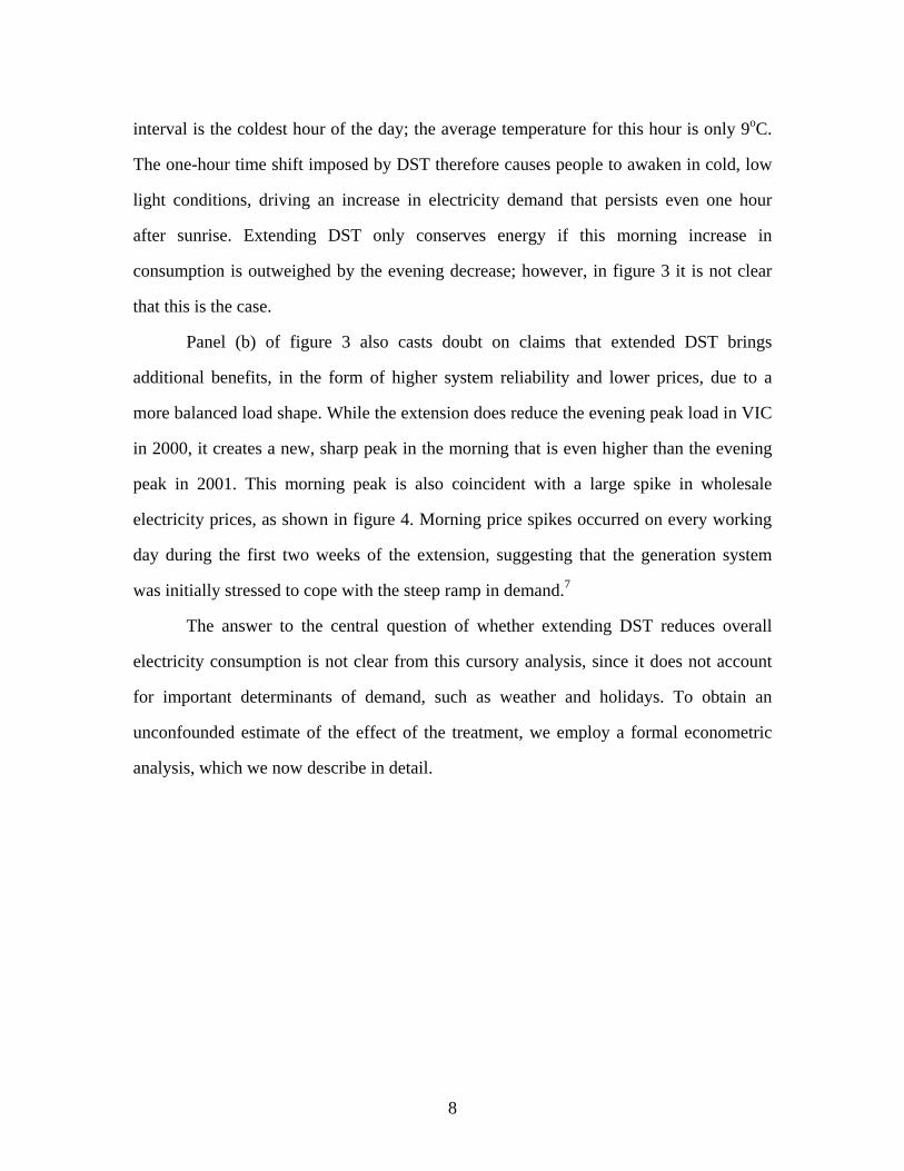
caused by the DST extension in each half-hour are displayed in figure 7, and presented in

tabular format in appendix C. Extending DST affects electricity consumption in a manner

consistent with the preliminary graphical analysis: there is a transfer of consumption from

the evening to the morning. This behavior agrees with the expected effects of DST’s one-

hour time shift. Less lighting and heating are required in the evening; however, demand

increases in the morning—particularly from 07:00 to 08:00—driven by reduced sunlight

and lower temperatures.

To assess whether the evening decrease in demand outweighs the morning

increase, we aggregate the half-hourly estimates using (2) to yield an estimate of θ. We

find that the extension of DST did not conserve electricity, as shown in the first column

15

of table 3. The point estimate of the percentage change in demand over the entire

treatment period is +0.11% with a clustered standard error of 0.39.

We also examine the impact of the DST extension separately for the pre-Olympic

and post-Olympic treatment periods, which we will now refer to loosely as September

and October. That is, we unpool each treatment dummy Tidh and estimate separate

coefficients Sephβ and Oct

hβ for each half-hour. Because September in the southern

hemisphere is seasonally equivalent to March in the northern hemisphere, this

examination has policy implications beyond Australia—recent efforts to extend DST in

the U.S. and California concern an extension into March, as DST is already observed in

April in these locations. Prior studies have found that such an extension reduces

electricity consumption by 1% in the U.S. and by 0.6% in California. In contrast, we

estimate that the extension of DST into September in Australia increased electricity

demand by 0.34%, as shown in table 3.14

To formally compare our estimates to the previous literature, we define three null

hypotheses: (1) θ = -1.0%, (2) θ = -0.6%, and (3) θ = 0.0%, and test whether they are

rejected by our estimates. Table 4 displays p-values for rejection of each null hypothesis

in a two-sided test, given both our pooled and unpooled results. Even with clustered

standard errors, our estimate of the effect of the DST extension in September rejects the

most modest energy savings estimate in the literature of 0.6% (CEC, 2001) at a 5% level.

Over the entire treatment period, we reject a 1% reduction in demand at a 1% level, and

reject a 0.6% reduction at a 10% level. These rejections are strengthened with the use of

Newey-West standard errors.

In summary, the results indicate that extending DST did not significantly reduce

electricity demand in VIC. In September in particular, the extension was more likely to

have increased than decreased electricity consumption.

16

5.2 Robustness

Our results are robust to many alternative specifications, as shown in table 5. Our

results are invariant to the choice between a weather model based on Bushnell and

Mansur (2005) and one from CEC (2001). Further, our results do not change appreciably

if we include years and months of data beyond what we use in our reference case, if we

use Queensland as a control state rather than SA, or if we estimate (1) in standard time

rather than clock time. This robustness is underlined by the precise fit of our model: the

adjusted R2 across all models is greater than 0.94.

Regression equation (1) contains over 1800 parameters. While the point estimates

and the standard errors for the parameters of primary interest—the treatment effects—are

discussed above, most of the other coefficients are significant and carry signs that agree

with intuition. For example, weekends, holidays, and vacations lower electricity

consumption, and deviations from the base temperature of 18oC increase electricity

consumption, consistent with the effects of air-conditioning (when above 18oC) and

heating (when below 18oC).

The weights ωh used to calculate θ̂ are based on the average of the 1999 and

2001 half-hourly demands. As an alternative set of weights, we also use the estimated

half-hourly counterfactual demand in 2000, given by exp{XVICdhαVICdh + WVICdhφih}⋅ VICdq .

Doing so does not affect our estimate of θ.

As a final check of our estimates, we evaluate whether extending DST causes a

relatively greater reduction in electricity consumption on weekends and holidays than on

working days. This would be consistent with the intuition that, on non-working days, less

early activity mitigates the morning increase in demand. We estimate that electricity

consumption on working days increased by 0.4% during the extension, while

17

consumption on weekends and holidays decreased by 0.9%. This difference is significant

at the 5% level.

6. Evaluation of the simulation technique

It is natural to ask is whether the simulation technique used by CEC (2001) to

predict energy savings in California would have accurately predicted the outcome of the

Australian DST extension. A successful validation would lend credence to the model’s

results in California, and suggest that California and the rest of the U.S. may experience

reduced energy use due to an extension, even if Australia did not.

The simulation approach uses data on hourly electricity consumption under the

status quo DST policy to simulate consumption under a DST extension. This procedure

first employs a regression analysis using status quo data to assess how electricity demand

in each hour is affected by weather and light, and then uses the regression coefficients to

predict demand in the event of a one-hour time shift, lagging the weather and light

variables appropriately. The consistency of the simulation results relies on the assumption

that extending DST will not cause patterns of activity that are not observed in the status

quo. This may not hold in practice. For example, to simulate demand under extended

DST at 07:00 in March in the U.S., the model must rely on observed status quo behavior

at 07:00 under similarly cold and low-light conditions. Without a DST extension, these

conditions are observed only in mid-winter. The simulation will be inaccurate if people

behave differently in the morning in mid-winter than they do in spring under extended

DST.

In contrast, in the Australian quasi-experiment, we have already estimated the

effect of the DST extension directly, by comparing observations under both the status quo

and the extension. We can therefore evaluate the simulation’s performance by re-

18

estimating its first stage using status quo observations, forecasting electricity demand

under an extension, and then comparing these results to those estimated from actual data.

The first stage of the simulation model is a regression of hourly electricity

demand, qdh, on employment, weather, and astronomical sunlight and twilight variables,

for a full year of observations:

dhdhhdhhdhhdh uLightdWeathercEmploymentbaq ++++=

The disturbance ud is correlated across the h = 1,…,24 hourly equations per the

Seemingly Unrelated Regression method (Zellner, 1962). The regression allows the

weather and light coefficients to vary across the twenty-four hours of the day, and the

weather specifications are very detailed, involving several lags and moving averages of

half-hourly temperatures, with different coefficients for hot, warm, and cold conditions.15

Once the vectors of regression coefficients are estimated, they are used in the second

stage of the model to forecast electricity consumption under a DST extension. This is

accomplished by lagging the weather and light variables by one hour and by adding the

first stage realized error term to construct the following projection:

dhdhhdhhdhhsimdh uLightdWeathercEmploymentbaq ˆˆˆˆˆ 11 ++++= −−

We apply the first stage of the CEC model to the Australian data for all of 1999

and 2001, and then simulate electricity consumption under extended DST in VIC in

September 1999 and 2001 (we are unable to simulate demand under an extension in 2000

using the CEC’s method because we do not observe demand under Standard Time in that

year). Figure 8 illustrates the simulated demand, as well as actual demand (under

19

standard time), in both years. The simulations predict a substantial decrease in demand in

the evening and only a minor increase in demand in the morning, with overall energy

savings of 0.43% in 1999 and 0.41% in 2001. Both the hour-by-hour and overall results

closely align with the 0.6% savings predicted for California in the original study (see

Figure 9). The results disagree, however, with the actual outcome of the Australian DST

extension in 2000. Figure 8 also includes, in bold, the realized demand in VIC under the

2000 treatment. In both 1999 and 2001, the simulation fails to predict a morning increase

in electricity consumption similar to that observed in 2000, and also overestimates

evening savings. The simulated decrease in overall consumption is inconsistent with what

actually happened in VIC. Based upon our triple DID estimate of a 0.34% increase in

consumption in September presented earlier, we reject the simulated 0.41% savings at a

10% significance level. The simulation is unable to predict the substantial intra-day shifts

that occur due to the early adoption of DST, a result that holds even after we attempt to

improve the model’s fit by selecting a smaller first-stage sample in which light and

weather conditions most closely resemble the extension period in September.

7. Conclusions

Given the economic and environmental imperatives driving efforts to reduce

energy consumption, policy-makers in several countries are considering extending

Daylight Saving Time (DST), as doing so is widely believed to reduce electricity use.

Our research challenges this belief, as well as the studies underlying it. We offer a new

test of whether extending DST decreases energy consumption by evaluating an extension

that occurred in the state of Victoria, Australia, in 2000. Using half-hourly panel data on

electricity consumption and a triple-differenced treatment effect model, we show that,

while extending DST did reduce electricity consumption in the evening, these savings

20

were negated by increased demand in the morning. We further find that the extension

caused sharp peak loads and prices in the morning hours.

From an applied policy perspective, this study is of immediate interest for

Australia, which is actively considering using DST as a tool for energy conservation.

Moreover, the lessons from Australia may carry over to the U.S. and to California in

particular, as Victoria’s latitude and climate are similar to those of central California. The

planned extension that will occur in the U.S. in 2007 will cause DST to be observed in

March—a month that is analogous to September in Australia, when our results suggest

that DST increases rather than decreases electricity consumption. Further, we find that

the simulation model that supported a DST extension in California over-estimates energy

savings when we apply it to Australia. This casts suspicion on its previous policy

applications in the U.S., and provides further evidence that the planned U.S. extension is

unlikely to achieve its energy conservation goals.

21

References

Arellano, Manuel, “Computing Robust Standard Errors for Within-Groups Estimators,”

Oxford Bulletin of Economics and Statistics 49 (November 1987), 431-434.

Bertrand, Marianne, Esther Duflo, and Sendhil Mullainathan, “How much should we

trust differences-in-differences estimates?” Quarterly Journal of Economics 119

(February 2004), 249-275.

Bushnell, James B. and Erin T. Mansur, “Consumption under Noisy Price Signals: A

Study of Electricity Retail Rate Deregulation in San Diego,” Journal of Industrial

Economics 53 (December 2005), 493-513.

California Energy Commission (CEC), Effects of Daylight Saving Time on California

Electricity Use (Report P400-01-013, May 2001).

California Joint Senate Resolution. (Bill no. SJRX2-1, 25 June, 2001).

Downing, Michael, Spring Forward: The Annual Madness of Daylight Saving Time

(Washington, D.C.: Shoemaker & Hoard, 2005).

Emergency Daylight Savings Time Energy Conservation Act (U.S. Public Law 93-182,

December 1973).

Energy Policy Act of 2005 (U.S. Public Law 109-58, July 2005).

Franklin, Benjamin, “An Economical Project, Essay on Daylight Saving,” The Journal of

Paris (April 1784).

Hamermesh, Daniel S., Caitlin K. Myers, and Mark L. Pocock, “Time Zones as Cues for

Coordination: Latitude, Longitude and Letterman,” NBER Working Paper no.

12350 (2006).

Meyer, Bruce D., “Natural and Quasi-Experiments in Economics,” Journal of Business &

Economic Statistics 13 (April 1995), 151-161.

22

National Electricity Market Management Ltd. (NEMMCO), An Introduction to

Australia’s National Electricity Market (2005).

New South Wales Legislative Assembly Hansard, “Standard Time Amendment Bill,

Second Reading” (26 May 1999, article 40, and 2 June 1999, article 9).

New South Wales Legislative Assembly Hansard, “Standard Time Amendment (Daylight

Saving) Bill, Second Reading” (13 September 2005, article 44).

Newey, Whitney K. and Kenneth D. West, “A simple, positive definite,

heteroskedasticity and autocorrelation consistent covariance matrix,”

Econometrica 55 (May 1987), 703-708.

Outhred, Hugh, personal correspondence (20 July, 2006).

Prerau, David S, Seize the Daylight: The Curious and Contentious Story of Daylight

Saving Time (New York: Thunder’s Mouth Press, 2005).

Rock, Brian A., “Impact of daylight saving time on residential energy consumption and

cost,” Energy and Buildings 25 (February 1997), 63-68.

Scoop Independent News, “Minister Urged to Consider Early Daylight Saving” (14

August, 2001).

The Energy Conservation Center, Japan, Report on the National Conference on the

Global Environment and Summer Time (2006).

The Toronto Star, “Get set for darker November mornings” (p. A1, 21 July 2005).

United Kingdom House of Commons Hansard “Energy Saving (Daylight) Bill” (26

January 2007)

U.S. Department of Transportation (U.S. DOT), The Daylight Saving Time Study: A

Report to Congress by the US Department of Transportation (Washington, D.C.:

GPO, 1975).

U.S. Department of Energy, Energy Information Administration (U.S. EIA), Electric

Power Annual 2005 (DOE/EIA-0348 (2005), revised November 2006).

23

Vanduffel, Steven, “Comonotonicity: From Risk Measurement to Risk Management,”

Academisch Proefschrift, Faculteit der Economische Wetenschappen en

Econometrics, Amsterdam (2005).

Wooldridge, Jeffrey M., “Cluster-Sample Methods in Applied Econometrics,” American

Economic Review Papers and Proceedings 93 (May 2003), 133-138.

Zellner, Arnold, “An efficient method of estimating seemingly unrelated regression

equations and tests for aggregation bias,” Journal of the American Statistical

Association 57 (June 1962), 348–368.

24

Appendix A: Data processing

Electricity data are missing for occasional half-hours, so we estimate the missing

observations via interpolation using adjacent half hours. Weather data are also missing

for some occasional hours as well for four entire days (none of which fall in within the

treatment dates in any year, except for the air pressure variable). While we estimate

weather for isolated missing hours via interpolation, we estimate weather for unobserved

days via a regression analysis using information from the daily-level weather dataset.

Details and code for this procedure are available from the authors upon request.

Schedules for most school vacations, state holidays, and federal holidays were

obtained from the Australian Federal Department of Employment and Workplace

Relations, The Department of Education and Children's Services (SA), and The

Department of Education and Training (VIC). For years in which information was not

available from the above institutions, the dates were obtained by internet search.

Employment data were obtained from the Australian Bureau of Statistics’ Labor Force

Spreadsheets, Table 12. Sunrise, sunset, and twilight data were sourced from the U.S.

Naval Observatory, and the days and times of switches to and from DST were obtained

from the Time and Date AS Company.

While our data are provided in Standard Time, we conduct our analysis in clock

time. We therefore convert our data to clock time, which, for most affected observations,

requires a simple one-hour shift. However, at the start of a DST period, the 02:00-03:00

interval (in clock time) is missing. To avoid a gap in our data, we duplicate the 01:30-

02:00 information into the missing 02:00-02:30 half hour, and likewise equate the

missing 02:30-03:00 period to our 03:00-03:30 observation. Further, when a DST period

terminates, the 02:00-03:00 period (in clock time) is observed twice. Because our model

is designed for only one observation in each half-hour, we average these observations.

25

Appendix B: Justification of using 12:00 to 14:30 as the control period

Our identification strategy uses the assumption that electricity demand in the mid-

day is not affected by DST. The purpose of this appendix is to offer regression results to

justify this assumption and to explain our choice of 12:00 to 14:30 as the base demand

period for setting q in equation (1).

In VIC and SA, we observe “typical” switches from standard time to DST in late

October of 1999 and 2001-2005. These observations allow us to examine DST’s effect on

mid-day electricity consumption by performing a regression discontinuity analysis of

demand near the date of each switch. Specifically, we form a regression sample

consisting of half-hourly demand observations during the week before and week after the

switch to DST in each year. We then regress, separately for each half-hour, the logarithm

of demand on an indicator variable for when DST is in effect, state-specific within-year

time trends, fixed effects for the interaction of state and year, fixed effects for day of

week, fixed effects for holidays and vacations, and weather variables.

Before discussing the estimated effect of DST in the mid-day, we first note that

this specification produces estimates which show that DST increases demand in the

morning and decreases demand in the evening. For example, during 07:00-07:30, we

estimate that demand increases by 5.9% following the switch to DST, with a standard

error of 1.0% (we report standard errors clustered on year, though these are not

appreciably different from OLS standard errors). During 18:30-19:00 we estimate a

decrease in demand of 4.9%, with a standard error of 1.7%. The signs and statistical

significance of these results are consistent with intuition, and indicate that this

specification has sufficient statistical power to resolve non-zero effects where they exist.

In the mid-day, however, the effect of switching to DST is statistically

insignificant. Table B displays estimates of the percentage effect of switching to DST,

along with standard errors, for several half-hour intervals. These results are robust to the

26

addition of another week of data before and after each switch to DST, and to the addition

of quadratic state-specific within-year time trends. The point estimates are smallest in

magnitude from 12:30-14:00, and increase both before and particularly after this time

period.

Selection of this 12:30-14:00 interval as the base period for estimation of the main

specification, equation (1), ultimately yields an estimate of θ of +0.3% (which is

statistically indistinguishable from zero). Expanding the base period symmetrically

around 12:30-14:00 includes within it hours of the day in which our regression

discontinuity estimates in table B indicate that DST is likely to increase demand.

Therefore, as we expand the base period, the estimates of θ decrease. This is

demonstrated by the fact that the reference case estimate of θ, which uses the longer

12:00-14:30 interval as the base period, is +0.1%. We choose this interval to be our base

period, rather than 12:30-14:00, to be conservative in our final estimate.

27

Appendix C: Half-hourly estimation results

Table C displays the estimated percentage impact of the DST extension on

electricity demand in each half hour: these are the point estimates given by 1)ˆexp( −hβ

and correspond to figure 6. Note that the large effects in the late-night hours are caused

by centralized off-peak water heaters in Melbourne (Outhred, 2006). These are triggered

by timers set on Standard Time—groups of heaters are activated at 23:30 and 01:30. Each

turns off on its own once its heating is complete. During the DST extension, each heater

turns on one hour “late” (according to clock time). This drives the negative, then positive,

overnight treatment effects. Regressing equation (1) in standard time, rather than clock

time, eliminates these overnight effects, and produces a point estimate that the extension

increased overall electricity consumption by 0.4%.

28

Notes

1 Historically, DST has been most actively implemented in times of energy scarcity. The

first application of DST was in Germany during World War I. The U.S. observed

year-round DST during World War II and implemented several extensions during

the energy crisis in the 1970s (Emergency Daylight Savings Time Energy

Conservation Act, 1973). Today, DST is observed in over seventy countries

worldwide. For more information on the history of DST, see the recent books by

Prerau (2005) and Downing (2005). 2 See NSW Legislative Assembly Hansard (2005), The Toronto Star (2005), The Energy

Conservation Center, Japan (2006), Scoop Independent News (2001), and U.K.

House of Commons (2007).. 3 Rock (1997) also uses a simulation model, and finds that year-round DST decreases

electricity consumption by 0.3% and expenditures by 0.2%. However, his study

does not include non-residential electricity use, which accounts for 64% of U.S.

total electricity consumption (U.S. EIA, 2005). 4 NEMMCO data can be obtained at http://www.nemmco.com.au/data/market_data.htm 5 The “zigzag” pattern that occurs between 23:00 and 02:00 in both states is due to

centralized off-peak water heating that is activated by automatic timers, set to

standard time (Outhred, 2006). 6 Hamermesh et al. (2006) examine spatial coordination externalities triggered by time

cues. Their results imply that SA in 2000 may have adjusted its behavior in

response to the treatment in VIC. In particular, their model predicts that people in

SA would awaken earlier in the morning to benefit from aligning their activities

with their neighbors in VIC. However, the effects that Hamermesh et al. calculate

are small, and panel (a) of figure 3 does not show evidence of such a time shift.

29

7 Because the Australian electricity market is integrated across state boundaries, demand

shocks in VIC caused by extended DST affect not only wholesale prices in VIC, but

also prices in SA. We therefore do not undertake a formal analysis of extended

DST’s effect on prices, because a control state does not exist. 8 To further analyze whether visitors before and after the Olympic Games spent extended

vacations in VIC or SA, we collected tourism information. These data show that,

while NSW was affected by tourism during the Olympics, VIC and SA were

unaffected. Data are available from the authors upon request. 9 The specification is the same as equation (1), as described in section 4.2, except that

mid-day demand is not subtracted from the left-hand-side. 10 Our final specification pools some hours to improve efficiency of the weather models.

This does not impact the reported estimates of the treatment effects. 11 Heating degrees are calculated as the difference between the observed temperature and

18.33oC (65oF). The motivation of squaring the heating degree is that, as the

temperature deviates from 18.33oC, cooling or heating efforts increase nonlinearly.

This functional form is consistent with other electricity demand models in the

literature (see Bushnell and Mansur 2005). 12 To derive this, we make use of the assumption that mid-day demand is invariant to the

treatment. 13 50 lags allow the errors to be correlated over slightly more than one full day. Tests of

AR(p) models on ε suggest that the disturbances are correlated over the first six

hours of lags, but not beyond that. However, the coefficient on the 48th lag is

significant. Also, note that the triple DID specification considerably decreases the

autocorrelation of the dependent variable, relative to a standard DID.

30

14 The point estimate in October is that the extension reduces electricity demand by

0.06%. While the difference between the September and October estimates is

significant at only the 30% level, the sign of the difference is intuitive: in October

there is more morning sunlight and temperatures are warmer, so the morning

increase in demand is mitigated.

15 Details of the definition on these variables, the estimation of the model, and the

simulation are explained in CEC (2001). We make minor changes to the CEC

specification to account for our half-hourly, rather than hourly data, and for the fact

that we observe humidity, precipitation, and daily unobstructed sunshine, but not

hourly cloud cover. Computer code is available from the authors upon request.

Figure 1: Southeastern Australia states and major cities

NSW, VIC, and SA in mainland Australia regularly begin DST on the last Sunday in October each year. In 2000, however, NSW and VIC began DST on 27 August, whereas SA did not begin DST until 29 October.

NSW, VIC, and SA in mainland Australia regularly begin DST on the last Sunday in October each year. In 2000, however, NSW and VIC began DST on 27 August, whereas SA did not begin DST until 29 October.

Capital State

Capital population in

millions

State population in

millions

State income per capita in 1000 AUD

Latitude South

Longitude East

Average sunrise

Average sunset

Sydney NSW 4.3 6.5 41.4 33°5' 151°1' 5:50 17:45Melbourne VIC 3.7 4.8 39.3 37°47' 145°58' 6:20 18:10Adelaide SA 1.1 1.5 33.4 34°55' 138°36' 6:50 18:35

All data are for 2000. Sunrise and sunset times are in East Australian Standard Time, and averaged during September

Table 1: Characteristics of capital cities in southeast Australia

Figure 2: Timeline of 2000 events in New South Wales, Victoria, and South Australia

27 August:DST starts inNSW and VIC

29 October:DST starts in

SA

15 September – October 1:Sydney Olympics in NSW

27 August:DST starts inNSW and VIC

29 October:DST starts in

SA

15 September – October 1:Sydney Olympics in NSW

State Variable [unit] Mean Std dev Mean Std dev Mean Std devDemand [MW] 5131.86 528.87 5347.71 554.17 5405.90 553.66Price [AUD/MWh] 19.22 6.34 43.30 179.29 29.11 84.04Temperature [Celsius] 13.51 4.46 12.12 3.90 12.11 3.73Precipitation [mm/hour] 0.07 0.50 0.14 0.73 0.05 0.24Wind [meter/sec] 4.72 2.94 5.57 2.92 4.69 2.61Pressure [hPa] 1018.18 6.30 1011.97 7.17 1012.09 6.17Sunshine [hours/day] 6.78 3.89 5.90 3.71 5.78 3.43Humidity [percent] 71.02 17.18 72.51 15.83 72.58 17.11Employment [in 1000] 2192.72 14.14 2272.06 12.05 2289.02 11.46Non-Working Day [% of days] 0.31 0.46 0.24 0.43 0.33 0.47School-Vacation [% of days] 0.00 0.00 0.00 0.00 0.09 0.28Holiday [% of days] 0.00 0.00 0.00 0.00 0.00 0.00Demand [MW] 1324.23 185.70 1398.49 201.43 1428.66 197.66Price [AUD/MWh] 54.12 166.53 56.27 178.97 27.50 17.85Temperature [Celsius] 15.95 4.81 14.41 3.69 13.48 3.20Precipitation [mm/hour] 0.00 0.00 0.12 0.54 0.12 0.48Wind [meter/sec] 4.22 2.53 5.05 2.87 4.73 2.88Pressure [hPa] 1017.93 6.53 1014.51 6.89 1013.79 6.32Sunshine [hours/day] 8.53 3.12 7.20 3.54 6.38 3.31Humidity [percent] 62.99 19.20 68.52 17.76 70.46 16.93Employment [in 1000] 668.76 2.69 684.22 2.43 682.85 2.33Non-Working Day [% of days] 0.42 0.49 0.27 0.44 0.44 0.50School-Vacation [% of days] 0.11 0.31 0.00 0.00 0.20 0.40Holiday [% of days] 0.02 0.15 0.02 0.15 0.00 0.00

Table 2: Summary statistics: 1999-2001, treatment dates only

Abbreviations: MW = Megawatts; AUD/MWh = Australian Dollars per Megawatt-hour; mm = millimeters; hPa = Hectopascal. Note that the maximum wholesale electricity price is capped at 5000 AUD/MWh from 1999-2000, and at 10,000 AUD/MWh in 2001. The cap is designed to mitigate generator market power (NEMMCO, 2005).

Sout

h A

ustra

lia

2160 observations per state, per year1999 2000 2001

Vic

toria

Figure 3: Average half hourly electricity demand in South Australia and Victoria during the treatment dates

1000

1200

1400

1600

Con

sum

ptio

n in

Meg

awat

ts

0 2 4 6 8 10 12 14 16 18 20 22 24Hour

1999 20002001

4200

4600

5000

5400

5800

Con

sum

ptio

n in

Meg

awat

ts

0 2 4 6 8 10 12 14 16 18 20 22 24Hour

1999 20002001

Hour (Standard Time) Hour (Standard Time)

(a) South Australia (control) (b) Victoria (treated in 2000)

Figure 4: Average half hourly electricity prices and demand in Victoria during the treatment dates

4500

5000

5500

6000

010

020

030

040

050

0P

rice

in D

olla

rs p

er M

Wh

0 2 4 6 8 10 12 14 16 18 20 22 24Hour (Standard Time)

Con

sum

ptio

n in

Meg

awat

ts

Prices199920002001

Demand2000

4500

5000

5500

6000

010

020

030

040

050

0P

rice

in D

olla

rs p

er M

Wh

0 2 4 6 8 10 12 14 16 18 20 22 24Hour (Standard Time)

Con

sum

ptio

n in

Meg

awat

ts

Prices199920002001

Demand2000

Prices199920002001

Demand2000

Figure 5: Ratio between average VIC demand and average SA demand during the treatment dates, 1999-2005

1

1.1

1.2

1.3

1.4

1.5

1.6

1.7

0 2 4 6 8 10 12 14 16 18 20 22

Hour (Standard Time)

Log(

VIC

dem

and

/ SA

dem

and)

1999200020012002

200320042005

1

1.1

1.2

1.3

1.4

1.5

1.6

1.7

0 2 4 6 8 10 12 14 16 18 20 22

Hour (Standard Time)

Log(

VIC

dem

and

/ SA

dem

and)

1999200020012002

200320042005

1999200020012002

200320042005

Figure 6: Ratio between average VIC demand and average SA demand, August through November, 1999-2005

1.2

1.25

1.3

1.35

1.4

1.45

1999 2000 2001 2002 2003 2004 2005

log(

VIC

Dem

and)

- lo

g(SA

Dem

and)

01 Aug - 26 Aug

Treatment dates

28 Oct - 30 Nov

Figure 7: Half hourly effects of extending DST on electricity use

-10.0

-8.0

-6.0

-4.0

-2.0

0.0

2.0

4.0

6.0

8.0

10.0

6 7 8 9 10 11 12 13 14 15 16 17 18 19 20 21 22

Hour (Clock Time)

Perc

ent C

hang

e in

Con

sum

ptio

n

95% confidence intervals are indicated, with standard errors clustered by day.

All days September OctoberWorking

daysNon-working

daysPercent change in demand 0.11 0.34 -0.06 0.44 -0.94

Standard error (0.39) [0.32] (0.43) [0.34] (0.43) [0.36] (0.40) [0.33] (0.41) [0.40]

Clustered standard errors are in parentheses and Newey-West standard errors are in brackets

Table 3: Summary of estimated treament effects, aggreagated over all half-hours

Null hypothesis

Clustered std error

Newey-West

Clustered std error

Newey-West

Clustered std error

Newey-West

θ = -1.0% 0.002 0.000 0.029 0.009 0.004 0.001

θ = -0.6% 0.030 0.006 0.208 0.131 0.067 0.026

Electricity neutrality θ = 0.0% 0.430 0.319 0.891 0.870 0.776 0.729

Electricity savings

Table 4: p-values for rejection of electricity saving hypotheses

September estimate (+0.34%)

October estimate(-0.06%)

Pooled estimate(+0.11%)

Reference case

CEC weather

Include data to 2005

Include Aug and Nov

Queensland as control

state

Run in Standard

TimePercent change in demand 0.11 0.00 0.20 0.39 0.18 0.39Clustered standard error (0.39) (0.38) (0.35) (0.35) (0.28) (0.40)

Table 5: Summary of robustness tests of the pooled specification

Figure 8: Actual and simulated electricity consumption in VIC, September 1999-2001

Figure 9: Simulation of DST in California, March 1998-2000 (CEC, 2001)

Status quo demand is observed under Standard Time.

11:00- 11:30- 12:00- 12:30- 13:00- 13:30- 14:00- 14:30- 15:00-11:30 12:00 12:30 13:00 13:30 14:00 14:30 15:00 15:30

Percent change in demand 1.41 0.44 0.66 0.19 -0.24 0.40 1.35 1.33 1.31Standard error (1.74) (1.43) (1.56) (1.54) (1.41) (1.64) (1.90) (1.37) (1.56)

Standard errors are clustered on year

Half-hour

Table B: Regression discontinuity estimates of the effect of switching to DST, by half-hour:late-October switches in VIC and SA in 1999 and 2001-2005

Half-hour beginning at βh

Standard error

t-statistic exp(βh)-1

Half-hour beginning at βh

Standard error

t-statistic exp(βh)-1

00:00 -0.012 0.007 -1.77 -0.012 12:00 0.000 0.002 0.19 0.00000:30 0.019 0.007 2.75 0.019 12:30 -0.001 0.001 -0.71 -0.00101:00 -0.050 0.006 -7.66 -0.048 13:00 -0.006 0.001 -4.72 -0.00601:30 -0.045 0.007 -6.81 -0.044 13:30 -0.003 0.001 -2.48 -0.00302:00 0.055 0.006 8.53 0.057 14:00 0.009 0.002 5.25 0.00902:30 0.076 0.006 12.10 0.079 14:30 0.013 0.003 5.31 0.01303:00 0.073 0.006 11.31 0.075 15:00 0.010 0.003 3.08 0.01103:30 0.068 0.007 10.27 0.071 15:30 0.008 0.004 2.09 0.00804:00 0.057 0.006 8.77 0.059 16:00 0.009 0.005 1.97 0.00904:30 0.045 0.006 7.19 0.046 16:30 0.002 0.005 0.41 0.00205:00 0.032 0.006 5.16 0.033 17:00 -0.014 0.006 -2.32 -0.01405:30 0.025 0.006 4.18 0.025 17:30 -0.027 0.007 -3.63 -0.02606:00 0.019 0.006 3.23 0.019 18:00 -0.048 0.007 -6.48 -0.04706:30 0.015 0.006 2.58 0.015 18:30 -0.066 0.007 -8.84 -0.06407:00 0.079 0.006 12.87 0.082 19:00 -0.055 0.008 -7.08 -0.05407:30 0.077 0.006 12.70 0.080 19:30 -0.026 0.008 -3.33 -0.02508:00 0.024 0.006 3.82 0.024 20:00 -0.008 0.008 -1.04 -0.00808:30 0.006 0.005 1.23 0.006 20:30 -0.005 0.008 -0.62 -0.00509:00 0.004 0.005 0.79 0.004 21:00 0.001 0.007 0.13 0.00109:30 0.002 0.004 0.48 0.002 21:30 0.005 0.007 0.68 0.00510:00 0.000 0.004 0.01 0.000 22:00 -0.006 0.007 -0.85 -0.00610:30 0.003 0.003 1.06 0.003 22:30 -0.027 0.006 -4.33 -0.02611:00 0.000 0.003 0.13 0.000 23:00 -0.124 0.007 -18.69 -0.11711:30 0.001 0.002 0.33 0.001 23:30 -0.129 0.007 -18.24 -0.121

Standard errors are clustered on date

Table C: Estimated treatment effects by half-hour