November, 2004

The Effect of Infrastructure on Long Run Economic Growth

David Canning

Harvard University

and

Peter Pedroni *

Williams College

--------------------------------------------------------------------------------------------------------------------Abstract: We investigate the long run consequences of infrastructure provision on per capita income in apanel of countries over the period 1950-1992. Simple panel based tests are developed which enable us toisolate the sign and direction of the long run effect of infrastructure on income in a manner that is robustto the presence of unknown heterogeneous short run causal relationships. Our results provide clearevidence that in the vast majority of cases infrastructure does induce long run growth effects. But we alsofind a great deal of variation in the results across individual countries. Taken as a whole, the resultsdemonstrate that telephones, electricity generating capacity and paved roads are provided at close to thegrowth maximizing level on average, but are under-supplied in some countries and over-supplied inothers. These results also help to explain why cross section and time series studies have in the past foundcontradictory results regarding a causal link between infrastructure provision and long run growth. --------------------------------------------------------------------------------------------------------------------

JEL Classifications: O1, H4.

* Corresponding author: The current version of this paper was completed while the second author was appointed asthe Clayton Fellow of the Baker Institute and a visitor in the Economics Department at Rice University, and theauthor is grateful for their hospitality. Address correspondence to Peter Pedroni, Baker Institute and Department ofEconomics, Rice University, 6100 Main St., Houston, TX 77005, pedroni@rice.edu.

** Acknowledgments: This paper has been funded in part by the World Bank and in part by the USAID CAER IIproject whose assistance is gratefully acknowledged. The views and interpretations expressed in this paper are thoseof the authors and should not be attributed to either the World Bank or USAID. We would like to thank EsraBennathan, George vonFurstenberg, Eric Leeper, Gary Madden, Salvador Ortigueira and Lucie Schmidt for theircomments. We also thank seminar participants at the Bank of England, Indiana University, SUNY Albany,Williams College, the North American Summer Meetings of the Econometric Society, the Cornell-Penn StateAnnual Macro Conference, and the Midwest Macro Meetings at the University of Pittsburgh.

1. Introduction

We address the issue of whether stocks of infrastructure are at, above, or below their growth

maximizing levels. Our approach is based on the growth model of Barro (1990). Infrastructure

capital is an input into aggregate production, but it comes at the cost of reduced investment in

other types of capital. In this approach there is an optimal level of infrastructure which

maximizes the growth rate; if infrastructure levels are set too high they divert investment away

from other capital to the point where income growth is reduced.

This model implies a simple “reduced form” relationship between income per capita and

infrastructure stocks per capita. Below the growth maximizing infrastructure level positive

shocks to infrastructure will tend to increase the level of output, while above the optimal level,

positive infrastructure shocks will tend to reduce the level of output; this can identify where each

country’s infrastructure stock stands relative to the growth-maximizing level.

Kocherlakota and Yi (1996, 1997) use a related approach to study the relationship between

shocks to public capital and subsequent changes in GDP in the United States and the United

Kingdom over the last 100 years and our approach is builds upon their methodology. We use the

same intuition for the causal connection between infrastructure and growth, but our work has

several distinguishing features. Perhaps most importantly is the distinction in our emphasis.

Kocherlakota and Yi are interested in the existence of a long run effect while we focus on the

sign of the effect. We estimate the effect for a large panel of countries using data from 1950 to

1992, allowing us to address the question of whether infrastructure levels have been too low, to

high, or about right over this period.

We also employ a number of innovations. Firstly, we use physical measures of

infrastructure, kilometers of paved roads, kilowatts of electricity generating capacity and number

of telephones rather than constructing stock estimates from investment flows. While simple

2

physical measures do not correct for quality, monetary investment in infrastructure may be a

very poor guide to the amount of infrastructure capital produced (see Pritchett (1996)).

Secondly, we find evidence of unit roots in both the GDP per capita (as do Cheung and Lai

(2000) and Lee, Pesaran and Smith (1997)) in the infrastructure data that we employ. Such unit

roots can be removed by taking first differences but this ignores the long run relationship in the

data if the series are cointegrated. We find that GDP per capita and infrastructure stocks are

cointegrated, and by exploiting this cointegrating relationship we develop a simple approach to

isolating the long run effect from the short run effects. Our panel approach also permits us to

compare cross country averages of these effects.

We find that in general both short run and long run causality is bi-directional, with

infrastructure responding to GDP per capita but GDP per capita also responding to infrastructure

shocks. Most importantly, we find evidence of a long run impact of infrastructure on GDP per

capita. For telephones and paved roads, the sign of the effect of an increase in provision on GDP

per capita varies across countries, being positive in some but negative in others. On average

telephones and paved roads are supplied at around the growth maximizing level, but some

countries have too few while others have too many. It follows that the appropriate policy at the

country level will depend on country specific studies. Our finding that some countries actually

have too much infrastructure is consistent with Devarajan, Swaroop and Zou (1996) and Ghali

(1998), who find evidence of over provision of public capital in a number of developing

countries. We find that long run effects of investment in electricity generating capacity are

positive in a large number of countries, with negative effects being found in only a few. This

suggests that, on average, electricity may be under provided.

Our approach allows us to make inferences based on a very simple reduced form

3

(1)

relationship. This avoids the problems of estimating the effect of infrastructure on output in a

more fully specified structural growth model (e.g. see Easterly and Rebelo (1993), Garcia-Mila,

McGuire and Porter (1996), Gramlich (1994), Holtz-Eakin (1994), Holtz-Eakin and Lovely

(1996), Holtz-Eakin and Schwartz (1995), Ghali (1998), Turnovsky and Fisher (1994), Morrison

and Schwartz (1996)). While our approach has the advantage of simplicity, it tells us only the

direction of the net effect of infrastructure on growth, not its magnitude.

In the next section we present a stylized growth model to motivate the empirical approach

that is undertaken in this study. In particular, we derive our simple estimated relationship as a

reduced form of a growth model. In section 3, we carry out panel-based unit root and

cointegration tests to characterize the time series properties of our data that are relevant for our

subsequent analysis. Finally, in section 4 we discuss how we test for the sign and the direction

of long effects between our variables and present the results of these tests.

2. A Stylized Growth Model with Infrastructure Capital

Our model is adapted from Barro (1990). We add stochastic disturbances to his structural

equations and investigate how this affects the reduced form. The simple model form presented

here is for illustrative purposes. As we shall see, our estimation procedure actually allows for a

somewhat more general structure. Aggregate output Y, at time t, is produced using

infrastructure capital, G, other capital, K , and labor, L such that

where is total factor productivity at time t. For simplicity we assume a constant savings rate,

4

(2)

(3)

(4)

(5)

s, and that both types of capital fully depreciate each period. Next period’s infrastructure is a

proportion of savings (perhaps through a tax system or by a private sector mechanism that

channels investment based on private returns), so that

Investment in non-infrastructure capital is determined by

Substituting the capital accumulation equations (2) and (3) into the production function (1)

produces a difference equation for the evolution of per capita output

To complete the model, we need to describe the evolution of technical progress, , the share of

investment going to infrastructure, , and the size of the workforce, . We assume that each

of these is determined by an exogenous stochastic process. We model the log of total factor

productivity, as

where for some , and is a stationary random variable with .

Thus, log total factor productivity depends on a constant, , a trend rate of growth, , which

we take to be zero when , plus a random term that is stationary if and non-stationary if

.

We assume that the proportion of investment going to infrastructure is where

5

(6)

(7)

(8)

is a zero mean stationary series. Finally we assume that the growth rate of population is given

by , where is a zero mean stationary series. We further assume that

we can identify the workforce with the total population. Alternatively, we can easily weaken

this to an assumption that the labor force participation rate is a stationary series. Under these

assumptions, our difference equation can then be written in terms of log income per capita, y, as

where and .

Note that all the random terms in equation (6) are stationary, except possibly total factor

productivity, . According to equation (6) the process for contains a unit root whenever

and , or and . We require that one of these two mechanisms

operates to explain the very persistent unit root type behavior in per capita income that we

observe in the data, but we remain agnostic as to which one is appropriate for any particular

country of our sample.

Similarly, the process for infrastructure formation can be written in log per capita form as

We can rewrite this as

If has a unit root, is stationary, as are the remaining error terms in the relationship. In

this case, g and y are cointegrated, since a linear combination of g and y produces a stationary

variable. This will be true regardless of which assumption we use to generate the unit root in y.

6

1 In Barro’s model this is also the welfare maximizing infrastructure level. However, in thepresence of shocks, increasing expected growth may also increase the volatility of the growth rate.If agents are risk averse, maximizing expected growth need not maximize expected welfare.

However, in the exogenous growth version, the driving force behind growth is technical

progress, and long run infrastructure levels simply follow income levels. In the endogenous

growth model, on the other hand, there is the possibility that shocks to infrastructure investment

have permanent effects on the level of income.

Furthermore, the sign of this permanent effect may be positive or negative, depending on

whether has been set above or below the tax rate that maximizes expected growth. Note that

expected growth is maximized when the average share of investment in infrastructure is set at

the level that maximizes the expected value of . In general

this depends on the distribution of the shocks. However, without shocks, setting

maximizes the growth rate, as in Barro (1990).1 We assume a fixed savings rate so that

investment in infrastructure represents a diversion from other types of capital. In practice,

setting a sub-optimal level of reduces the rate of return to capital as a whole and may reduce

the savings rate and further lower the growth rate. Furthermore, it is important to notice that by

treating the savings rate as fixed, we are in effect taking the key margin over long periods to be

the allocation between different types of investment, rather than between the total level of

investment and consumption.

We now summarize each of these results in the following proposition.

7

Proposition 1. For the model specified by equations (1) through (8),

( ) If and , or and , then:

log per capita output, , and log per capita infrastructure series, , will each be non-stationary and integrated of order one, but there will exist a cointegrating vector (possiblydifferent for each country) such that some linear combination of and will be stationary.Shocks to productivity have a long run positive effect on log per capita output .

(ii) If and , then:

shocks to per capita infrastructure, , have no long run effect on per capita output, y.

(iii) If and , then:

shocks to per capita infrastructure, , will have a nonzero long run effect on per capitaoutput, . For small shocks, the sign of this effect will be positive if , and negative if

.

The proof of proposition 1 is straightforward and can be found in the longer working paper

version of this study, Canning and Pedroni (1999). In the neoclassical version of the model,

shocks to infrastructure have no long run effect. In the endogenous growth version of the model,

a positive shock to infrastructure increases income per capita when , and decreases income

per capita when . It should be noted that all of our results are for small changes to

infrastructure investment, since large changes could conceivably move the system across the

optimal infrastructure level into a different regime.

Given these results for the reduced form structure of the model, we can estimate a bivariate

relationship between income per capita and infrastructure stocks per capita, and test which

version of the model best describes the long run properties of the data. The model described in

this section represents a typical country of our data set. To apply the model to a panel of

8

countries we assume that all variables and innovations terms in the model carry a double index

to represent the value of the variable in country at time t. Furthermore, any parameters of

the model are assumed to be indexed by an subscript, so that we allow all of these to vary

across countries. These include for example, the income share parameters of the production

function, and , the savings rate, s, the average share of infrastructure investment , and the

persistence of the technology shock .

Finally, we should emphasize that for our empirical implementation, we simply require that

the data be characterized by the properties described in the results of proposition 1. This

characterization can be expected to apply to a broad class of similar models.

3. The Data

Our data are annual and cover the period 1950-1992. We use GDP per worker from the Penn

World Tables 5.6 (see Summers and Heston (1991)). The infrastructure data are from Canning

(1998), which gives physical infrastructure measured on an annual basis, in kilometers of paved

road, kilowatts of electricity generating capacity, and the number of telephones.

We deflate each variable by population so as to obtain per capita values, and then take logs

of these per capita values. This means we have variables representing log GDP per capita, log

paved roads per capita, log electricity generating capacity per capita, and log telephones per

capita. If the services provided by the infrastructure stocks are a rival good, then these simple

measures can be thought of as the average consumption of infrastructure services per capita. We

begin by investigating the time series properties of the data.

9

2As shown in the Monte Carlo studies reported in Pedroni (2004), nuisance parameters thatare associated with the serial correlation properties of individual member country time series areeliminated asymptotically as T grows large relative to N, which suggests that we should give moreweight to the time dimension when balancing the panel in order to avoid size distortion. The powerof the tests, on the other hand, rises most dramatically with the N dimension, and rapidly approaches100% against stationary but near unit root alternative hypotheses for the estimated residuals, evenin relatively short panels.

3.1 Testing for Unit Roots

We wish to test for non-stationarity against the alternative that the variable is trend

stationary, where we allow different intercepts and time trends for each country. We use the unit

root test proposed by Im, Pesaran and Shin (2003), which allows each panel member to have a

different autoregressive parameter and short run dynamics under the alternative hypothesis of

trend stationarity. To carry out the unit root and cointegration tests, we select countries and

time periods for each variable to construct a balanced panel, which entails a trade-off between

the time span and number of countries in the sample.2 For income per capita and electricity

generating capacity we take as our period 1950-1992. However for telephones and paved roads

we limit the period to 1960-1990 and 1961-1990 respectively, in order to get a reasonable

number of countries into the sample. When we come to look at the bivariate relationship the

coverage of the data set is always the same as for the infrastructure variable. As suggested by

Im, Pesaran and Shin, before carrying out the tests the data are purged of any common effects

across countries by regressing each variable on a set of time dummies and taking residuals.

The results of these unit root tests for each of our variables are shown in table 1. The test is

based on the average of the adjusted Dickey-Fuller (ADF) test statistics calculated independently

for each member of the panel, with five lags to adjust for auto-correlation. The adjusted test

statistics, (adjusted using the tables in Im, Pesaran and Shin (2003)) are distributed as N(0,1)

10

(9)

under the null of a unit root, and large negative values lead to rejection of a unit root in favor of

stationarity.

In no case can we reject the null hypothesis that every country has a unit root for the series in

log levels. We then test for a unit root in first differences, though in this case the alternative

hypothesis is stationarity without a trend, since any time trend in levels is removed by

differencing. When we use first differences, the test statistic is negative and significant in each

case. This indicates that we have stationarity in first differences and each of the four variables

can be regarded as I(1). In what follows we will proceed on the assumption that all log level

variables are I(1) and all log differenced variables are I(0).

3.2 Testing for Cointegration

Now we turn to the question of possible cointegration between each infrastructure variable

and GDP per capita. Given the possibility of reverse causality between the variables we use

panel cointegration technique from Pedroni (1999, 2004) which is robust to causality running in

both directions and allows for both heterogeneous cointegrating vectors and short run dynamics

across countries. In particular, the cointegrating regression that we estimate is

so that each country has its own relationship between git , the log per capita infrastructure

variable, and yit , log per capita income. The variable eit represents a stationary error term. Note

that we allow the slope of the cointegrating relationship to differ from unity and to vary across

countries. This reflects the fact that in practice the relationship between infrastructure

investment, infrastructure stocks, and income per capita may be more complex than set out in

11

equation (2). Furthermore, this allows for the possibility that in practice, growth need not be

balanced, so that the ratio of capital stocks to output need not be one. The common time

dummies, bt , capture any common worldwide effects that would tend to cause the individual

country variables to move together over time. These may be either relatively short term business

cycle effects, or longer run effects such as worldwide changes in technology that may affect the

relative costs or benefits of infrastructure and thus the equilibrium relationship.

The residuals of this regression are used to construct an ADF based group mean panel

cointegration test which is analogous to the Im, Pesaran and Shin (2003) ADF unit root test. In

table 2 we report the average over countries of the ADF t-test calculated from the residuals from

regression (9) with a lag length of up to 5 years. Adjustment values to construct the test statistic

are from Pedroni (2004), which allows for the fact that we are testing residuals from an

estimated relationship rather than the true relationship. Large negative values imply stationarity

of the residuals and lead to a rejection of no cointegration. As the results make clear, we reject

the null of no cointegration in each of the three cases. Consequently, in what follows we will

proceed on the assumption that each of our series is non-stationary, but that there is cointegration

between each infrastructure variable and GDP per capita.

4. Long Run Effects; Empirical Implementation and Econometric Issues

Having established a long run relationship between infrastructure and income we now turn to the

issue of causality. In particular, we are interested in whether innovations to infrastructure stocks

have a long run effect on GDP per capita and what the sign of such an effect is. We begin this

section by setting out tests for the presence and sign of such long run effects and then proceed to

carry out these tests on our data.

12

(10)

Since in each country the series g and y are individually non-stationary but together are

cointegrated, we know from the Granger representation theorem, (Engle and Granger, (1987))

that these series can be represented in the form of a dynamic error correction model. To estimate

the error correction form we employ a two step procedure. In the first step, we estimate the

cointegrating relationship between log per capita income and log per capita output given in

equation (9) for each country, using the Johansen (1988, 1991) maximum likelihood procedure.

In the second step, we use this estimated cointegrating relationship, to construct the

disequilibrium term, We then estimate the error correction model

The variable eit represents how far our variables are from the equilibrium relationship and the

error correction mechanism estimates how this disequilibrium causes the variables to adjust

towards equilibrium in order to keep the long run relationship intact. The Granger representation

theorem implies that at least one of the adjustment coefficients must be non-zero if a

long run relationship between the variables is to hold.

By proposition (1), shocks to income have a persistent, positive component. Furthermore,

the Granger representation theorem places restrictions on the singular long run response matrix

of the moving average representation for the data in differences. This restricts the relationship

between the long run response matrix and the speed of adjustment coefficients in the

error correction representation. We can exploit these two pieces of information to test for the

existence, and the sign, of any long run causal effects running from innovations in log per capita

13

infrastructure to log per capita output. We summarize our results in the following proposition;

the derivation can be found in the longer working paper version of this study, Canning and

Pedroni (1999).

Proposition 2. Under the specification of our growth model,

(I) The coefficient, , on the lagged equilibrium cointegrating relationship in the dynamic errorcorrection equation for is zero if, and only if, innovations to log per capita infrastructurehave no long run effect on log per capita output.

(ii) The ratio of the coefficients, , on the lagged equilibrium cointegrating relationship inthe dynamic error correction equations for and , has the same sign as the long run effectof innovations to log per capita infrastructure on log per capita output.

It follows from proposition 2 that we can test hypotheses about the long run effect of

infrastructure on output by testing restrictions on the estimated coefficients in the dynamic error

correction equations. According to proposition 2, a test for the significance of for any one

country can be interpreted, conditional on our growth model, as a test of whether innovations to

per capita infrastructure have a long run effect on per capita output, and a test for the sign of the

ratio can be interpreted as a test of the sign of the long run effect of innovations to per

capita infrastructure on per capita output. Note that proposition 2(ii) need not necessarily hold

for cointegrated systems in general; the proof relies both on the Granger representation theorem

and specific features of the growth model set out in section 2.

The advantage of our two step estimation procedure, first estimating the cointegrating

relationship and then the error correction mechanism, is that all the variables in equation system

(10) are stationary. Asymptotically, the fact that we use the estimated disequilibrium rather than

the true disequilibrium in (10) does not affect the standard properties of our estimates, due to the

14

3Toda and Phillips (1993) study these properties in the context of more conventional dynamicGranger causality tests in cointegrated systems. See also Urbain (1992) for a related discussion ontesting causality in error correction models.

4 See, for example, Faust and Leeper (1998) for a discussion of these issues. Furthermore,as Phillips (1998) demonstrates, inferences for such long horizon impulse responses are verysensitive to misspecification of the underlying unit root and cointegration properties of the data.

well known superconsistency properties of the estimator of the cointegrating relationship.3 It

follows that we can carry out standard hypothesis tests on the coefficients estimated in the

system.

By exploiting the cointegrating relationship we are able to summarize the long run effects of

the innovations in the variables in terms of two parameters, and . This contrasts with

using the differenced variables in a stationary vector autoregressive (VAR) representation to

estimate the impulse responses over long horizons. The tradeoff is that we only test for the

existence and sign of long run effects rather than obtaining a quantitative measure of the size of

these effects. On the other hand, as is well known, the standard errors for VAR based estimates

of impulse responses over long horizons are notoriously large and unreliable, making inference

difficult.4 In essence, by exploiting the cointegrating relationships present in the data, and

summarizing the long run effects of our growth model in a small number of parameters, we

avoid the problems of inference that are typically associated with summing sequences of impulse

response coefficients over a long horizon.

4.1 Causality Tests

We now turn to the empirical results of our tests. However, before implementing these tests

for long run causal effects, we begin by asking a simpler question. We test whether the

15

5 Under the null of no causality, the percentage of countries rejecting at 10% significancelevel has an expected value of 10 with a standard deviation of 30N-1/2 (for N large). Using thisdistribution, the number of countries in which we reject no causality is significantly greater thanexpected even at the 1% level.

coefficients on lagged infrastructure changes and the error correction adjustment parameter in

the regression explaining income changes are all zero. This is a test of no causal effect from

infrastructure shocks to income either in the short run or the long run. We also test for causality

running in the other direction from income to infrastructure. These tests correspond to the usual

Granger causality tests in that they are tests of whether one variable evolves entirely

exogenously from another.

Column two of table 3 reports the percentage of countries that reject an F-test of the

hypothesis of no causality at the 10% significance level. One interpretation of these results is

that causality seems to occur in some countries, but not in others. However, if there really were

no causality, we would expect to reject this hypothesis, and accept causality in 10% the of

countries, if we use the 10% significance level for our test. Rejection in a larger number of

countries can be taken as evidence against the hypothesis that there is no causality in any

country. Using this criterion, we have strong evidence in favor of causality running in both

directions between each of our infrastructure variables and GDP, since we find rejections of no

causality in a great deal more than 10% of countries.5

A test of the joint hypothesis of no causality in any country is given in column three of table

3. This is a likelihood ratio test of the hypothesis that all the relevant parameters are zero in

every country. Under the null of no causality the test statistic is distributed as chi-squared with

degrees of freedom equal to the number of restrictions imposed, which is given in parentheses

beneath the statistic. Large values of this statistic lead to rejection of the null hypothesis of no

16

causality. Again, evidence supports two-way causality between these variables and GDP per

capita and each of our infrastructure variables. The fact that non-causality is rejected in a

significant number of countries supports the idea that the results for the likelihood test of non-

causality in any country are not being driven by a small number of extreme estimates in a few

countries.

4.2 Tests for the Presence of Long Run Effects

The conventional Granger causality results indicate two way feedback. However, the

causality associated with this feedback may be only of a short run nature, so that innovations to

infrastructure have an impact on GDP per capita from business cycle or multiplier effects that

eventually die out and do not have a lasting effect on long run growth.

Therefore, we now turn to the issue of whether infrastructure investment affects long run

economic growth. Since our variables are cointegrated, proposition 2 gives us some simple

tests. The first test that we consider is a joint test of the hypothesis that the adjustment

parameter is zero in every country, i.e. that there is no long run effect of infrastructure on

income. We report the results of this test in column 1 of table 4. This likelihood ratio test

provides strong evidence against the long run effect being uniformly zero among all countries,

and easily rejects the null of no long run effect at the 1% significance level in each case.

4.3 Tests for the Sign of the Long Run Effect

First, we ask whether the parameters are homogeneous across countries. In table 5 we report the

results for tests of homogeneity of the long run adjustment parameters across countries. The test

17

6 This is only a test that for all , but it is easy to check that the test statistic is largerfor any other test of the form . It follows that if we reject for all , we reject for all , for any choice of

(11)

that we use for homogeneity is a Wald test. For a parameter , the test statistic is calculated as

where is the weighted mean of the country specific parameters (weighted by the inverse of

their variances).6 Using this test, we decisively reject homogeneity of across countries.

Furthermore, when we test the ratio , which we call the sign parameter, we reject

homogeneity for telephones and paved roads, though in this case only at the 10% significance

level. However, it is interesting to note that we do not reject homogeneity of the sign parameter

across countries in the case of electricity. These results are important when we interpret our tests

for the sign of the long run effects.

Given the likelihood of heterogeneity of the parameter estimates across countries, we now

examine the distribution of these estimates (rather than simply pooling them and examining the

sign of the average). The first column of table 6 gives the weighted means of the sign parameter

estimates across countries, with weights given by the inverse of the estimated coefficient

variance. The average estimated value is close to zero.

This suggests that the long run effects of increased provision of telephones and paved roads

on growth are close to zero on average across countries, but that there are significant nonzero

long run effects in individual countries. We can see this when we look at column 2, of table 6.

While the average of the sign parameter is zero for telephones, a significantly greater number of

countries reject a zero parameter than should occur by chance. In columns 3 and 4 of table 6 we

18

perform one sided tests where the alternative to no effect is a negative and a positive effect

respectively. The number rejecting non-causality for telephones in favor of a positive effect and

in favor of a negative effect are both significantly larger than would be predicted by pure

sampling variation and are approximately equal to one another. It follows that while telephones

appear to have long run effects, the direction of the effect varies across countries. This implies

that some countries are below, while others are above, their optimal level of provision of

telephones relative to the growth maximizing level.

For paved roads we get a similar result with the mean of the sign parameter being close to

zero and some countries have significant positive, and some significant negative, effects.

However, the number of countries with significant negative effects, at 21%, is somewhat larger

indicating the possibility that negative effects, and oversupply of roads, is the more common

condition.

In the case of electricity generating capacity, the fact that we do not reject homogeneity of

the sign parameter leads to a somewhat different interpretation of the results in table 6. It

implies that it is possible to interpret the mean as an estimate of a single parameter that holds in

each country. However, we again find it hard to determine the sign of the mean; while we

estimate a positive effect, it is not significantly different from zero. This implies electricity is

supplied at about its optimal level. The number of individual countries producing rejections of a

zero value for the sign parameter is also not greater than we would anticipate based on pure

sampling variation, which is consistent with the idea that the actual parameters are actually all

zero. However, in one sided tests, there are a significant number of countries where shocks to

electricity generating capacity tend to have a positive effect on long run economic growth. It

appears that electricity generating capacity is under provided in some countries. Overall, for

19

electricity the results are consistent with all countries being at the optimal level of provision,

though there is some evidence of positive effects of electricity on long run growth rates in some

countries.

One potential source of heterogeneity in our results is that we are pooling countries at very

different levels of income per capita. Disaggregating by income group we find very similar

results to those we have reported for the whole sample, though there is some evidence that paved

roads are more likely to have a positive effect on income growth in developing countries while

the positive effect of electricity provision is mainly found among richer countries. (See the

longer working paper version of this study, Canning and Pedroni (1999) for further details).

5. Conclusion

Infrastructure must be paid for. According to our model, there is a growth maximizing level of

infrastructure above which the diversion of resources from other productive uses outweighs the

gain from having more infrastructure. Below this level, increases in infrastructure provision

increase long run income, while above this level an increase in infrastructure reduces long run

income. It follows that we can use the effect of shocks to infrastructure provision on long run

income levels as a test of where a country’s infrastructure stock stands relative to its optimum

level from a growth maximizing perspective. This is conceptually a very simple test since it

does not rely on knowing the full structure of the system being examined.

Our results are interesting from the point of view of economic policy. Rather than simply

asking whether there is evidence for a strong relationship between public infrastructure and long

run incomes, we are able to isolate the presence of an effect of infrastructure on income while

controlling for the reverse effect that income levels are likely to have on infrastructure provision.

20

7 For example Bils and Klenow (2000) provide strong evidence for the quantitativeimportance of controlling for the effect of growth on education when examining the effect ofeducation on growth.

Furthermore, by identifying the sign of this long run effect our approach allows for the fact that

infrastructure provision may divert resources from other forms of non-infrastructure investment

and asks whether the level of provision is likely to be above or below the optimum from a

growth maximizing perspective. In this context, it will be interesting in future research to

explore whether other forms of public investment such as education stand relative to their

growth maximizing levels.7 Finally, we are able to show that allowing for heterogeneity across

countries is also very important for policy purposes; average results for groups of countries tend

to disguise large differences between countries.

For telephones and paved roads we find no evidence of a worldwide infrastructure shortage.

For these, we find that on average countries are near the growth maximizing levels of

infrastructure provision, although a significant number of countries are over providing while in

others there is under provision. For electricity generating capacity our results can be taken to

support the view that countries are all close to the optimal level of provision, though we do have

some evidence of under provision in some countries.

In some ways our results are not surprising. If infrastructure were provided in competitive

markets, and there were no externalities present, this optimality result would be exactly what we

would expect. However, in practice, infrastructure has often been supplied by the public sector,

and we have the possibility of large externalities, perhaps leading to misallocation of resources.

In this context it could be said that the finding of optimality, even if just on average, is more

surprising. For policy purposes our results point to the need for detailed country studies of the

21

type employed by Fernald (1999) in order to find appropriate rates of return to infrastructure.

References

Barro R. J. (1990), “Government Spending in a Simple Model of Endogenous Growth,” Journalof Political Economy, Vol. 98, pp 103-125.

Bils, M. and Klenow, P. (2000), “Does Schooling Cause Growth?” working paper, University ofRochester.

Canning D. (1998), “A Database of World Infrastructure Stocks, 1950-1995,” World BankEconomic Review, Vol. 12, pp 529-547.

Canning D. and Pedroni P. (1999), “Infrastructure and Long Run Economic Growth”, Center forAnalytical Economics Working Paper No. 99-09, Cornell University.

Cheung Y.-W. and Lai K. (2000), International Evidence on Output Persistence from PostwarData, forthcoming in Economics Letters.

Devarajan S., Swaroop V. And Zou H. F. (1996), “The Composition of Public Expenditure andEconomic Growth,” Journal of Monetary Economics, Vol. 37, pp 313-344.

Easterly W. and Rebelo S. (1993), “Fiscal Policy and Economic Growth: An EmpiricalInvestigation,” Journal of Monetary Economics, Vol. 32, pp 417-458.

Engle R. F. and Granger C. W. J. (1987), “Co-integration and Error Correction: Representation,Estimation, and Testing,” Econometrica, Vol. 55, pp 251-276.

Faust, J. and Leeper E. (1998), “When do Long-Run Identifying Restrictions give ReliableResults?” Journal of Business and Economic Statistics, Vol. 15, pp 345-354.

Fernald J.G. (1999), “Roads to Prosperity?, Assessing the Link Between Public Capital andProductivity,” American Economic Review, Vol. 89, pp 619-638.

Garcia-Mila T., McGuire T. J. and Porter R. H. (1996), “The Effect of Public Capital in StateLevel Production Functions Reconsidered,” Review of Economics and Statistics, pp 177-180.

Ghali K. H. (1998), “Public Investment and Private Capital Formation in a Vector Error-correction Model of Growth,” Applied Economics, Vol. 30, pp 837-844.

Gramlich E. M. (1994), “Infrastructure Investment: A Review Essay,” Journal of EconomicLiterature, Vol. XXXII, pp 1176-1196.

22

Holtz-Eakin D. (1994), “Public Sector Capital and the Productivity Puzzle,” Review ofEconomics and Statistics, Vol 76, pp 12-21.

Holtz-Eakin D. and Lovely M.E. (1996), “Scale Economies, Returns to Variety and theProductivity of Public Infrastructure,” Regional Science and Urban Economics, Vol. 26, pp 105-123.

Holtz-Eakin D. and Schwartz A.E. (1995), “Infrastructure in a Structural Model of EconomicGrowth,” Regional Science and Urban Economics, Vol. 25, pp 131-151. Im K. S., Pesaran M. H. and Shin Y. (2003), “Testing for Unit Roots in Heterogeneous Panels,”Journal of Econometrics, 115, 53-74.

Johansen S. (1988), "Statistical Analysis of Cointegration Vectors", Journal of EconomicDynamics and Control, Vol. 12, pp 231-254.

Johansen S. (1991), "Estimation and Hypothesis Testing of Cointegration Vectors in GaussianAutoregressive Models", Econometrica, Vol. 59, pp 155-1580.

Kocherlakota N.R. and Yi K.M. (1996), “A Simple Time Series Test of Endogenous VersusExogenous Growth Models: An Application to the United States,” Review of Economics andStatistics, Vol. 78, pp 126-134.

Kocherlakota N. R. and Yi K. M. (1997), “It is there Endogenous Long-run Growth? Evidencefrom the United States and the United Kingdom,” Journal of Money Credit and Banking, Vol.29, pp 235-262.

Lee K., Pesaran M.H. and Smith R. (1997), “Growth and Convergence in a MulticountryEmpirical Stochastic Solow Model,” Journal of Applied Econometrics, Vol. 12 pp 357-392.

Morrison C.J. and Schwartz A.E. (1996), “State Infrastructure and Productive Performance,”American Economic Review, Vol. 86, pp 1095-1111.

Pedroni P. (2004), “Panel Cointegration; Asymptotic and Finite Sample Properties of PooledTime series Tests, With an Application to the PPP Hypothesis,” Econometric Theory, 20, 597-625.

Pedroni P. (1999), “Critical Values for Cointegration Tests in Heterogeneous Panels withMultiple Regressors,” Oxford Bulletin of Economics and Statistics, Vol. 61, pp 653-670.

Phillips P. C. B. (1998), “Impulse Response and Forecast Error Variance Asymptotics inNonstationary VARs,” Journal of Econometrics, Vol. 83, pp 21-56.

23

Pritchett L. (1996), “Mind Your P's and Q's, The Cost of Public Investment is Not the Value ofPublic Capital,” Policy Research Working Paper, No. 1660, Policy Research Department, WorldBank.

Summers R and Heston A. (1991), “The Penn World Table (Mark 5): An Expanded Set ofinternational Comparisons, 1950-1988,” Quarterly Journal of Economics, Vol. 106, pp 327-336.

Toda H. Y. and Philips P. C. B. (1993), “Vector Autoregression and Causality,” Econometrica,Vol. 61, pp 1367-1393.

Turnovsky S. J. and Fisher W. H. (1995), “The Composition of Government Expenditure and itsConsequences for Macroeconomic Performance,” Journal of Economic Dynamics and Control,Vol. 19, pp 747-786.

Urbain J. P. (1992) “On Weak Exogeneity in Error Correction Models,” Oxford Bulletin ofEconomics and Statistics, Vol. 54, pp 187-208.

24

Table 1Panel Unit Root Tests

Variable Period Number ofcountries

AverageADF

TestStatistic

log GDP per Capita 1950-1992 51 -2.164 -1.116

log EGC per Capita 1950-1992 43 -1.908 0.160

log TEL per Capita 1960-1990 67 -1.333 4.192

log PAV per Capita 1961-1990 42 -1.815 0.291

∆ log GDP per Capita 1951-1992 51 -2.465 -3.465***

∆ log EGC per Capita 1951-1992 43 -2.688 -4.863***

∆ log TEL per Capita 1961-1990 67 -2.172 -2.310**

∆ log PAV per Capita 1962-1990 42 -2.889 -5.992***

Notes: The test statistics are distributed as N(0, 1) under the null hypothesis of non-stationarity. The statistics are constructed using small sample adjustment factors from Im,Pesaran, and Shin (1996). The symbols * (**,***) denote significance at 10%, (5%, 1%)levels.

EGC represents kilowatts of electricity generating capacity.TEL represents the number of telephones.PAV represents kilometers of paved roads.

25

Table 2Panel Cointegration Tests

Period Countries Average ADF Test Statistic

Y and TEL 1960-1990 67 -2.33 -3.04*** Y and EGC 1950-1992 43 -2.28 -2.02** Y and PAV 1961-1990 42 -2.27 -1.90**

Notes: The test statistics are distributed as N(0, 1) under the null hypothesis of nocointegration. The statistics are constructed using adjustment values from Pedroni (2004).The symbols * (**,***) denote significance at 10%, (5%, 1%) levels.

Table 3 Granger Causality Tests

Null Hypothesis: Number of countries rejecting Full SampleNo Causality Countries null at the 10% likelihood

N significance level ratio test(percentage)

Y does not cause TEL 67 37.7*** 850*** (335)

Y does not cause EGC 43 51.2*** 504***(215)

Y does not cause PAV 42 45.2*** 695***(210)

TEL does not cause Y 67 46.3*** 801***(335)

EGC does not cause Y 43 30.2*** 368***(215)

PAV does not cause Y 42 42.9*** 424***(210)

Notes: Under the null hypothesis of a parameter value of zero in every country, thepercentage rejecting at the 10% significance level has an expected value 10 with a standarderror of 30N-1/2 . The likelihood ratio test is distributed as chi-squared with the degrees offreedom given in parentheses. The symbols * (**,***) denote significance at 10%, (5%,1%) levels.

26

Table 4Tests for Presence of Long Run Effects

Null Hypothesis: No Long Run Effects from Infrastructure to IncomeTest of

Likelihood Ratio TestTEL to Y 325***

(67)EGC to Y 164***

(43)PAV to Y 211***

(42)

Notes: All test statistics are distributed as chi-squared under the null hypothesis, with thedegrees of freedom given in parenthesis. The symbols * (**,***) denote significance at10%, (5%, 1%) levels.

Table 5Tests of Parameter Homogeneity for Long Run Effects Across Countries

Null Hypothesis: Homogeneity of parameters across countries

Test of Test of

Wald Test Wald Test

TEL to Y 232*** 101***(67) (67)

EGC to Y 124*** 46(43) (43)

PAV to Y 153*** 57*(42) (42)

Notes: Test statistics are distributed as chi-squared under the null hypothesis, with thedegrees of freedom given in parenthesis. The symbols * (**,***) denote significance at10%, (5%, 1%) levels.

27

Table 6Distribution of Parameters

Group Mean Percentage of Countries Rejecting Null:(weighted)

Alternative:

TEL to Y -0.014 14.9* 16.4** 16.4**N=67 (0.023)

EGC to Y 0.024 14.0 9.3 16.3*N=43 (0.028)

PAV to Y 0.027 16.7* 21.4*** 9.5N=42 (0.061)

(Standard errors in parenthesis)

Notes: Under the null hypothesis of a parameter value of zero in every country, thepercentage rejecting at the 10% significance level has an expected value 10 with a standarderror of 30N-1/2 . The likelihood ratio test is distributed as chi-squared with the degrees offreedom given in parentheses. The symbols * (**,***) denote significance at 10%, (5%,1%) levels.

28

Mathematical Appendix

Proposition 1: (i) Using equation (6) it is easy to show that y has unit root under either

specification, and cointegration of y and g follows directly from equation (8). In equation (6),

when , exogenous technology, , follows a random walk, and innovations to productivity

have a permanent effect on y even when . When , the endogenous process for

output accumulation is no longer mean reverting, so that when exogenous technology is mean

reverting, with , innovations to productivity have a permanent effect on y. Finally, since

, positive innovations to productivity lead to positive long run effects.

(ii) Shocks to infrastructure, , only affect the steady state through their effect on y. But when

, variations in y eventually dissipate since the parameter in the difference equation (6) is

less than one.

(iii) In this case all shocks to output are permanent. The long run effect of an infrastructure

shock to log output per capita is the same as the short run effect and is given by

Hence

Evaluating this at , and setting we have

It follows that for small positive shocks to infrastructure raise output in both the short

run and the long run while for small positive shocks tend to reduce output. Q.E.D.

29

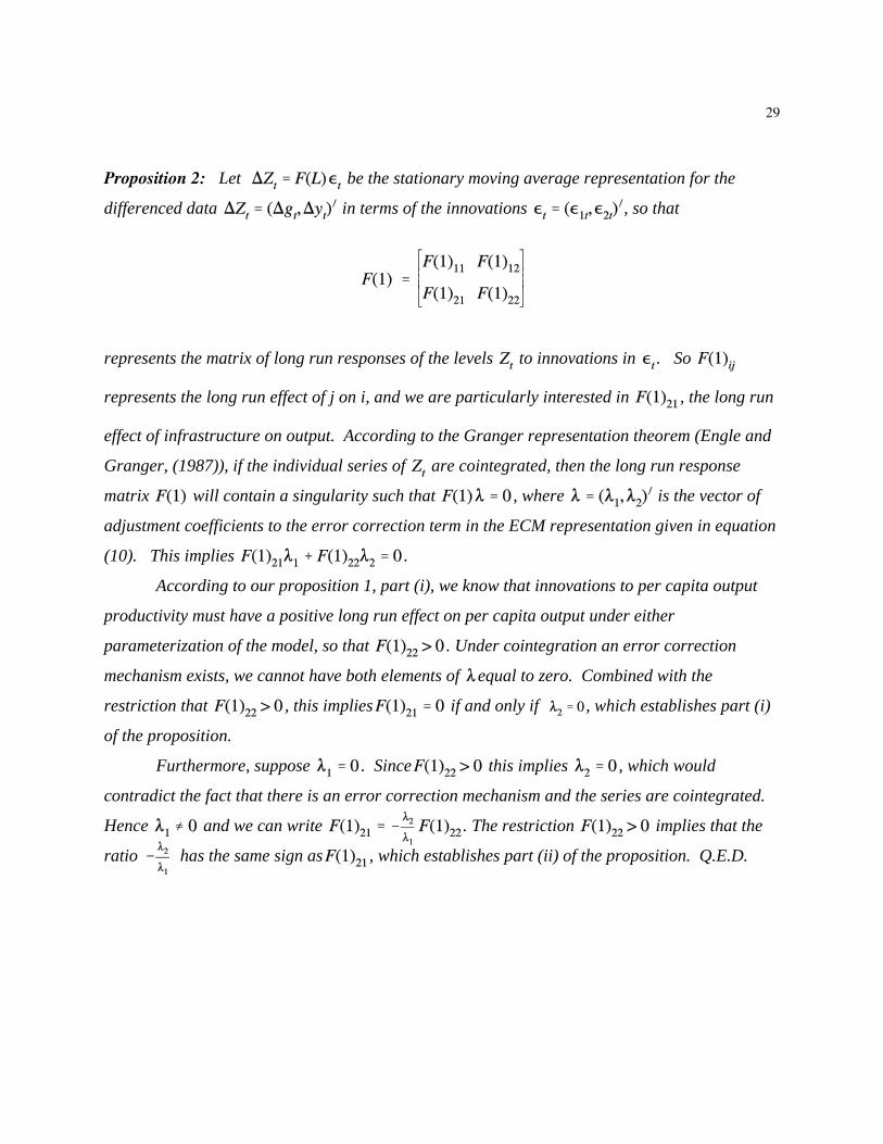
Proposition 2: Let be the stationary moving average representation for the

differenced data in terms of the innovations , so that

represents the matrix of long run responses of the levels to innovations in . So

represents the long run effect of j on i, and we are particularly interested in , the long run

effect of infrastructure on output. According to the Granger representation theorem (Engle and

Granger, (1987)), if the individual series of are cointegrated, then the long run response

matrix will contain a singularity such that , where is the vector of

adjustment coefficients to the error correction term in the ECM representation given in equation

(10). This implies .

According to our proposition 1, part (i), we know that innovations to per capita output

productivity must have a positive long run effect on per capita output under either

parameterization of the model, so that . Under cointegration an error correction

mechanism exists, we cannot have both elements of equal to zero. Combined with the

restriction that , this implies if and only if , which establishes part (i)

of the proposition.

Furthermore, suppose . Since this implies , which would

contradict the fact that there is an error correction mechanism and the series are cointegrated.

Hence and we can write . The restriction implies that the

ratio has the same sign as , which establishes part (ii) of the proposition. Q.E.D.