Does Monetary Policy Affect Stock Prices and Treasury Yields? An Error Correction and Simultaneous Equation Approach

J. Benson Durham* Division of Monetary Affairs

Board of Governors of the Federal Reserve System Mail Stop 71

20th and C Streets Washington, DC 20551

j.benson.durham@frb.gov

(202) 452-2896

Abstract This study pursues two addenda to the practitioner and academic on the effect of monetary policy on asset prices. First, this paper applies cointegration theory and, second, relaxes the stringent assumption in the literature that changes in 10-year Treasury yields, stock returns, and changes in the stance of monetary policy are exogenous. Given quarterly data from 1978:Q4 to 2002:Q3, two-stage least squares (2SLS) regressions suggest that changes in the exogenous component of the federal funds rate affect changes in Treasury yields but not stock returns, ceteris paribus. However, this result is sensitive to alternative proxies for the stance of monetary policy. Also, little evidence suggests that monetary policy responds to the exogenous components of changes in financial asset prices.

* Without implication, the author thanks Antulio Bomfim, Jim Clouse, Darrel Cohen, Brian Madigan, Athanasios Orphanides, and Brian Sack for helpful comments. The views expressed in this paper do not necessarily reflect those of the Board of Governors of the Federal Reserve System or any member of its staff.

1

1. Introduction

A large practitioner and academic literature examines the effect of monetary policy on

asset prices. Several studies address the impact of monetary policy surprises on daily or intraday

stock returns, for example, while fewer consider longer-run effects on equity prices and Treasury

yields. This research question has clear implications for both financial market participants and

central bankers. With respect to the former, the subject is of course germane to the broader issue

of empirical asset pricing, and practitioners spend considerable resources following (prospective)

monetary policy developments. Regarding the latter, the effect of monetary policy on equity

prices and interest rates is relevant to several possible transmission mechanisms from central

bank actions to the real economy. For example, the Federal Reserve controls the federal funds

rate, which purportedly affects market-determined interest rates and asset prices and, in turn, real

variables through various possible investment and consumption channels.

This paper pursues two addenda to previous studies on the effect of monetary policy on

stock prices and 10-year Treasury yields. First, the empirical literature, particularly regarding

policy transmission through the stock market, underutilizes error correction methodology. The

basic general intuition behind cointegration theory is that certain economic variables should not

diverge substantially in the long run. While such variables can drift apart in the short run,

economic forces eventually bring them together again (Granger, 1986, p. 213). An error

correction specification of stock prices and interest rates is perhaps particularly appealing with

respect to monetary policy, which should have transitory effects on asset prices. The long- and

short-run equations of a basic error correction model follow

(1)

Y*t = β0 + βXt + et

2

and

(2)

∆Yt = α0 + α1∆Xt + α2∆Zt + α3Μt – α4et-1 + µt,

respectively, where Y is the dependent variable, X is a set of explanatory variables in both

equations, Z is a set of variables that have transitory effects, M is a proxy for the stance of

monetary policy,1 and et-1 is the error correction term.

Second, previous studies of the response of asset prices over longer horizons to monetary

policy assume that stock prices, interest rates, and central bank policy are exogenous. But, asset

prices such as stocks and Treasury securities might be simultaneously determined, and asset

prices contain data about expectations for inflation and real activity that might, in turn, inform

monetary policy decisions. Therefore, this paper uses the error correction framework and treats

short-run changes in stock prices and Treasury yields, as well as the stance of monetary policy,

endogenously. Cointegration methodology is perhaps particularly useful in this regard, as the

error correction terms usefully instrument for the endogenous variables.

In general, these data indicate that monetary policy has somewhat limited impact on

financial asset prices. In particular, the exogenous component of the nominal federal funds rate

is a statistically significant determinant of 10-year Treasury yields, ceteris paribus, but other

proxies for the stance of monetary policy do not corroborate this finding. Moreover, few data

suggest that monetary policy responds to changes in asset prices. Some evidence suggests that

the exogenous component of 10-year Treasury yields correlates positively with the likelihood of

policy tightening episodes, but this result is also sensitive to proxy selection.

1 As noted below, hypotheses consider both the level and first difference of monetary policy proxies.

3

The next section reviews the literature on the longer-run effects of central bank policy on

stock returns and Treasury yields and presents the cointegration regression and unit root tests for

the long-run models of stock prices, interest rates, and monetary policy. Section 3 includes the

models for short-run dynamics, which follow simple instrumental variable (IV) techniques that

relax the assumption that financial asset price changes and monetary policy are exogenous.

Section 4 concludes.

2. Error Correction Models of Stock Prices, Interest Rates, and Monetary Policy

Before examining the short-run relations between asset prices and monetary policy, this

section focuses on long-run equilibrium models and the time-series properties of the data. The

discussion briefly outlines the literature on the effect of monetary policy on asset prices; reports

the results from unit root and mean stationarity tests of key variables; presents cointegrating

regressions for stock prices, 10-year Treasury yields, and the nominal federal funds rate; and

discusses the problem of simultaneity bias.

2.1. Stock Prices: Previous Literature and Cointegration Theory

Economists generally posit that restrictive (accommodative) monetary policy leads to

lower (higher) stock prices. For example, some researchers argue that changes in monetary

policy influence forecasts of market-determined interest rates, the equity cost of capital, and

expectations of corporate profitability (Waud, 1970). Others argue that central banks ease

(tighten) in responds to economic contraction (expansion), and therefore ex ante required and

realized ex post returns rise (fall) (Jensen and Johnson, 1995; Conover et al., 1999a, 1999b).

4

Some studies use high frequency data and document a correlation between monetary

policy changes and daily or intraday stock returns in the United States (Waud, 1970; Smirlock

and Yawitz, 1985; Cook and Hahn, 1988). With respect to the longer-run, Jensen and Johnson

(1995) examine monthly and quarterly performance and find that expected stock returns are

significantly greater during expansive monetary periods, and Conover et al. (1999a, 1999b) make

similar inferences using cross-country data. However, Durham (2001a, 2003) finds that these

findings are highly sensitive to alternative proxies for monetary policy; the use of excess as

opposed to raw stock returns; and sample selection, as more recent samples do not produce a

statistically significant relation.

In general, these time-series models of index returns follow

(3)

tlocaltt JDS εααα +++=∆ 210

where ∆St is the log difference of stock prices, Dt is a dummy variable equal to one (zero) if

prevailing local monetary regime is restrictive (expansive),2 and J is a set of control variables.

This paper extends this literature and, in contrast to (3), follows an error correction

specification of stock prices. As Harasty and Roulet (2000) argue,3 perhaps cointegration theory

is particularly germane to empirical models of stock market behavior – fundamental factors drive

market valuation in the long run, but in the short run, the market often substantially diverges

from its “fair” or fundamental value. Such short-run deviations are not sustainable, the argument

2 As Section 3 discusses in greater detail, this literature commonly expresses the policy variable in levels and the dependent variable in first differences, which is somewhat problematic. 3 For an earlier application of cointegration theory to stock prices see Campbell and Shiller (1987).

5

reasons, and eventually investors arbitrage the gap between fundamental fair value and short-run

market trends.4

Of course, determination of a fair value for stock prices is highly controversial, but for

these purposes, a simple present value model based on the widely cited Gordon-Shapiro formula

follows

(4)

( )gI

gDPt

tt −+

+=

θ1

where Dt is the current level of dividends, It is the long-run riskless rate of interest, g is the

growth rate of dividends, and θ is the equity risk premium. Following, Harasty and Roulet

(2000),5 who do not explicitly focus on the effect of monetary policy, the econometric

representation, expressed in logs, replaces dividends with earnings and simplifies the expression

of the discount factor. The corresponding empirical model and candidate long-run coingegrating

regression is therefore

(5)

St = β0 + β1EPSt + β2I10-yrt + eS

t

where St is the log level of the S&P 500, EPSt is the (log) one-year forward earnings-per-share

from IBES, I10-yrt is the 10-year Treasury yield, and eS

t is the error term.

4 The error correction term in (2) usefully addresses a particular shortcoming in (3). Even if accounting-based value measures are included in equation (3), time-series index models cannot adequately incorporate the effect of valuation measures on returns. First differences in, say, the price-to-earnings or price-to-book ratios are problematic in such specifications because changes in these measures are substantially driven by changes in stock prices, the dependent variable. Therefore, (3) cannot control for an important class of key supposed determinant of returns. In contrast, error correction methodology explicitly captures a more general “fair value.” The literature largely assesses the predictive power of accounting-based ratios such as price-to-book or price-to-earnings with cross-sectional firm-level data (i.e. Fama and French, 1992). 5 The variable that most closely measures the stance of monetary policy in their short-run regressions is the “relative variation” of short-term interest rates.

6

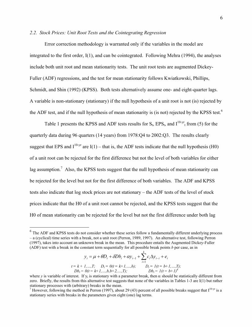
2.2. Stock Prices: Unit Root Tests and the Cointegrating Regression

Error correction methodology is warranted only if the variables in the model are

integrated to the first order, I(1), and can be cointegrated. Following Mehra (1994), the analyses

include both unit root and mean stationarity tests. The unit root tests are augmented Dickey-

Fuller (ADF) regressions, and the test for mean stationarity follows Kwiatkowski, Phillips,

Schmidt, and Shin (1992) (KPSS). Both tests alternatively assume one- and eight-quarter lags.

A variable is non-stationary (stationary) if the null hypothesis of a unit root is not (is) rejected by

the ADF test, and if the null hypothesis of mean stationarity is (is not) rejected by the KPSS test.6

Table 1 presents the KPSS and ADF tests results for St, EPSt, and I10-yrt from (5) for the

quarterly data during 96 quarters (14 years) from 1978:Q4 to 2002:Q3. The results clearly

suggest that EPS and I10-yr are I(1) – that is, the ADF tests indicate that the null hypothesis (H0)

of a unit root can be rejected for the first difference but not the level of both variables for either

lag assumption.7 Also, the KPSS tests suggest that the null hypothesis of mean stationarity can

be rejected for the level but not for the first difference of both variables. The ADF and KPSS

tests also indicate that log stock prices are not stationary – the ADF tests of the level of stock

prices indicate that the H0 of a unit root cannot be rejected, and the KPSS tests suggest that the

H0 of mean stationarity can be rejected for the level but not the first difference under both lag

6 The ADF and KPSS tests do not consider whether these series follow a fundamentally different underlying process – a (cyclical) time series with a break, not a unit root (Perron, 1989, 1997). An alternative test, following Perron (1997), takes into account an unknown break in the mean. This procedure entails the Augmented Dickey-Fuller (ADF) test with a break in the constant term sequentially for all possible break points b per case, as in

∑=

−− +∆++++=k

itititttt eycyDbDy

11αδθµ

t = k + 1,…,T; Dt = 0(t = k+1,…,b); Dt = 1(t = b+1,…,T); Dbt = 0(t = k+1,…,b,b+2,…,T); Dbt = 1(t = b+1)6

where y is variable of interest. If yt is stationary with a parameter break, then α should be statistically different from zero. Briefly, the results from this alternative test suggests that none of the variables in Tables 1-3 are I(1) but rather stationary processes with (arbitrary) breaks in the mean. 7 However, following the method in Perron (1997), about 29 (43) percent of all possible breaks suggest that I10-yr is a stationary series with breaks in the parameters given eight (one) lag terms.

7

assumptions. The ADF tests of ∆St are somewhat sensitive to lag assumption – inclusion of one

[eight] lagged terms suggests that St is I(1) [I(2)]. However, again, the level of St is clearly non-

stationary.

Table 4 presents the results from regression (5), the cointegrating regression. As Model

(1) indicates, β1 is safely statistically significant and positive with a coefficient notably greater

than unity, and β2 is similarly statistically significant with the anticipated negative sign and

suggests that stock prices fall about 6.5 percentage points with a 100-basis point increase in

interest rates. Therefore, these data suggest that in the long run stock prices are strongly related

to anticipated earnings and the level of interest rates. Also, returning to Table 1, the ADF test

results indicate that the H0 of a unit root can be rejected for the residual of this regression, eSt,

and the KPSS test suggests that the H0 of mean stationarity cannot be rejected. This further

suggests that St, EPSt, and I10-yrt can be cointegrated.8

Given that St, EPSt, and I10-yrt are I(1) and that the series can be cointegrated, short-run

regressions might follow

(6)

∆St = α0 + α1∆EPSt + α2∆I10-yrt + α3ΖS

t + α4∆Μt + α5eSt-1 + µt

where ZS includes additional variables that have transitory effects, ∆M is a proxy for the change

in the stance of monetary policy, and eSt-1 is the error correction term. ZS comprises several

factors, anomalous or otherwise, that previous index-level studies suggest correlate with stock

market returns (Durham, 2001b). These include three price history variables – one-month lagged

8 The sequential estimation of (1) and (2) or (5) and (6) follows Engle and Granger (1987) as well as Harasty and Roulet (2000) and differs from the method in Johansen (1988). This two-step method does not determine whether there is a unique cointegrating relation or a complex linear combination of all distinct cointegrating vectors in the system. As Harasty and Roulet (2000) note, one advantage of the two-step method is that it directly reflects the intuition behind long-run value and short-run deviations. Moreover, some studies (Campbell and Perron, 1991) suggest that the Johansen-Juselious (1990) method is highly sensitive to mis-specifiaction.

8

return, three- through 12-month lagged return (Jegadeesh, 1990), and the one-year lagged return

(De Bondt and Thaler, 1985) – and proxies for calendar effects – including dummy variables for

the January (Haugen and Lakonishok, 1987) and September (Siegel, 1998) effects.

The problem at this juncture, however, is that ∆St, ∆I10-yrt, and ∆Μt are perhaps

determined simultaneously, and an estimate of (6) should include instruments for ∆I10-yrt and

∆Μt. Therefore, the remainder of this section discusses the identification of ∆I10-yrt and ∆Μt.

2.3. Treasury Yields: Previous Literature and Cointegration Theory

Surprisingly few studies focus on the economic forces that determine the overall level of

interest rates (Sargent, 1969; Howe and Pigott, 1991; Mehra, 1994). But, Sargent (1969)

provides a useful framework for modeling the nominal interest rate, rnt, which is comprised of a

real equilibrium component, (ret); inflation expectations, (rn

t – rmt), expressed as the difference

between nominal and real market rates; and a term that measures the (expected) stance of

monetary policy, (rmt – re

t), expressed as the difference between the real market rate and the

equilibrium real interest rate. This sum follows

(7)

rnt = (re

t) + (rnt – rm

t) + (rmt – re

t).

The first term of (7), ret, is the equilibrium real rate that equates ex ante (private) savings

with investment and the government deficit (as well as the capital account in an open economy).

Investment, INV, and private savings, SAVPt, follow

(8)

INVt = a0 + a1∆Yt – a2ret

(9)

9

SAVPt = b0 + b1Yt + b2re

t

where Y is real income. Equation (8) is an accelerator-investment equation with interest rate

effects, and (9) is a Keynesian savings function.

In a closed economy equilibrium, which Sargent (1969) and Mehra (1994) consider, the

government surplus equals the excess of investment over private savings. In an open economy,

the government surplus equals the excess of investment and net exports over private savings, and

therefore ret solves

(10)

SAVGt = (INVt + NXt) – SAVP

t

where SAVGt is the government surplus to GDP, and NX is net exports to GDP.9 Substituting (8)

and (9) into (10) produces an expression for the equilibrium real interest rate, as in

(11)

( )[ ]tG

tte

t NXSAVYbYabaab

r +−−∆+−+

= 1110022

1

The government deficit (negative government savings), real income growth, and trade

surpluses raise the demand for funds and hence drive up ret, while a higher level of output

generates a larger volume of savings and hence reduces ret.

The second term of (7) is the gap between nominal and real interest rates, which arises

due to anticipated inflation following

(12)

rnt – rm

t = kπet

where πe is anticipated inflation.

9 The hypothesized sign for NX based on the identity is somewhat counterintuitive. For example, persistent trade surpluses can lead to a depreciation of the real exchange rate, which would necessitate a risk premium on domestic rates to attract investors.

10

The third term of (7) is the deviation of the real market rate from the equilibrium rate, rmt

– ret. This interest rate gap arises in part from monetary policy, as changes in the money supply

or some other monetary policy tool affect the demand and supply curves for funds following

(13)

rmt – re

t = -hiRMt,

where RM is a proxy for the real stance of monetary policy. More accommodative (restrictive)

monetary policy drives the market rate down (up) with respect to the equilibrium real rate.

Substituting (11), (12), and (13) into (7) produces a candidate cointegrating equation,

(14)

rnt = β0 +β1πe – β2RMt – β3SAVG

t – β4Yt + β5∆Yt + β6NX + ε,

which suggests that the nominal bond rate depends on anticipated inflation, changes in the real

stance of monetary policy, the (stock of the) government budget balance, changes in income, the

level of income, and net exports. However, some of these variables are possibly I(0) and do not

belong in the cointegrating relation.

2.4. Treasury Yields: Unit Root Tests and the Cointegrating Regression

Table 2 presents the ADF and KPSS tests for proxies for each of the right-hand-side

variables in (14). Following Howe and Pigott (1991), the proxy for inflation expectations is the

trailing 3-year average of (annualized) quarterly inflation.10 Following Mehra (1994), the proxy

for the real stance of monetary policy is the real federal funds rate. Total marketable federal

10 Results using the Michigan survey’s one-year ahead inflation expectations are available on request. The trailing 3-year average used in Tables 5-8, however, explains considerable more variance in nominal interest rates that the survey data.

11

government debt (to GDP) proxies SAVG.11 Also, given the positive correlation between

forward-looking EPS and income, the log of EPS proxies Y,12 and the excess of exports over

imports, divided by GDP, measures NX.

The results suggest that I10-yr (from Table 1), EPS (from Table 1), and NX are I(1). The

H0 of mean stationarity can (cannot) be rejected, and the H0 of a unit root cannot (can) be

rejected for the level (first difference) of these variables. The tests also suggest that πe is I(1),

and this result contradicts the view that inflation moves within a (target) range.13

Also, the data indicate that SAVG is non-stationary, but some tests suggest that SAVG

might be I(2) – the ADF test with eight lags suggests that the H0 of a unit root cannot be

rejected, and the KPSS with one lag test indicates that the H0 of mean-stationarity can be

rejected for ∆SAVG. Some tests suggest that the level of the real effect funds rate is stationary –

the ADF test with one lag suggests that the H0 of a unit root can be rejected, and the KPSS tests

that includes eight lags indicates that the H0 of mean stationarity cannot be rejected. Therefore,

the stationary variables from (14) – RM and ∆EPS – are not included in the cointegrating

regression, which therefore follows

(15)

I10-yrt = β0 +β1πe

t – β2SAVGt – β3EPSt + β4NXt + eI10-yr

t,

11 Results using the government deficit flow, which perhaps more closely follows the loanable funds model outlined in Section 2.3 are available on request. 12 Regressions that include the level and first difference of actual quarterly real output are available on request. However, in the context of 2SLS, these specifications suggest that ∆Y identifies changes in bond prices, while ∆EPS identifies changes in stock prices. However, Y and EPS both seem broadly related to the overall level of economic activity. 13 But, following Perron (1997), πe is stationary with breaks in the mean. About 25 (31) percent of all possible break points suggest that πe does not follow a unit root given eight (one) lag terms.

12

where eI10-yrt is the error term.

According to Model 2 in Table 4, the estimates are largely consistent with the

hypotheses, as β1, β2,1415 and β3 have the expected signs and are safely statistically significant.

However, the coefficient for NX, β4, is negative and safely significant, perhaps consistent with

an alternative hypothesis that higher levels of net exports lead to currency appreciation and lower

domestic interest rates. In addition, returning to Table 2, the residuals from this cointegrating

regression are I(0) – the H0 of mean stationarity cannot be rejected but that the unit root

hypothesis can be rejected.

Given that the independent variables in (15) are I(1), the corresponding model of short-

run dynamics follows

(16)

∆I10-yrt = α0 + α1∆πe

t – α2∆SAVGt + α3∆EPSt + α4∆NXt – α5∆St + α6∆Mt + α7eI10-yr

t-1 + µt,

where eI10-yrt-1 is the error correction term. But again, ∆St, ∆I10-yr

t, and ∆Μt are likely determined

simultaneously, and the discussion now turns to identification of ∆Μt.

2.5. Monetary Policy: The Taylor Rule, Unit Root Tests and the Cointegrating Regression

A large literature addresses both the descriptive and prescriptive aspects of the “Taylor

Rule” for monetary policy (Taylor, 1993), in which central bank policy responds to variations in

inflation and output. Very briefly, a very simple econometric representation of the rule follows

(17)

Mt = β0 + β1πet + β2ψt + eM

t

14 This result is of course highly germane to the debate regarding the effects of government spending on interest rates. Again, the proxy in this paper is the stock of total marketable federal government debt to GDP, which is not a measure of market expectations of future fiscal balances. 15

13

where a possible proxy for Mt includes the nominal federal funds rate, ψt is the output gap (the

difference between current and potential output), and eMt is an error term.

Again, πe is I(1) according to Table 2, and the ADF and KPSS results in Table 3 indicate

that the effective federal funds rate and ψ are also I(1). The result for the output gap is

somewhat surprising, as the concept concerns (temporary) deviations from potential output,

which presumably by construction revert back to potential (the mean). Therefore, one might

interpret (17) as a cointegrating relation only in a strict econometric sense, given that ψt is a

stationary concept. Nevertheless, Model 3 in Table 4 indicates that β1 and β2 both have the

expected positive signs and are safely statistically significant. Moreover, some data indicate that

eMt is stationary, which suggests that the variables in the simple Taylor Rule specification can be

cointegrated. (However, as Table 3 indicates, these results are somewhat sensitive to lag length,

as the H0 of a unit root cannot be rejected given the ADF test with eight lags, and the H0 of

mean stationarity can be rejected given the KPSS test with eight lags.)

The corresponding model of short-run dynamics follows

(18)

∆Mt = α0 + α1∆πet + α2∆ψt + α3∆St + α4∆I10-yr

t +α5∆Mt-1 +α6eMt-1+µt,

and notably includes ∆St and ∆I10-yrt, consistent with the view that financial asset prices might

very well inform central bank policy. In addition, the short-run specification includes lagged

changes in the federal funds rate to capture possible policy inertia.

Given specification of the cointegrating relations for St, I10-yrt, and Mt, the discussion now

turns to estimation of the exogenous components of the endogenous variables.

3. Short-run Dynamics

14

This section examines the short-run dynamics of the first differences in stock prices,

Treasury yields, and monetary policy. The discussion outlines the identification of the system of

equations; presents the 2SLS results, including the first stage regressions; and briefly examines

alternative proxies for the stance of monetary policy.

3.1. Identification of the 2SLS System

∆St, ∆I10-yrt, and ∆Mt can be identified given equations (6), (16), and (18), rewritten as

(19)

∆St = α0 + α1∆EPSt + α2∆I10-yrt + α3ΖS

t + α4∆Μt + α5eSt-1 + µt

∆I10-yrt = β0 + β1∆πe

t – β2∆SAVGt + β3∆EPSt + β4∆NXt – β5∆St + β6Mt + β7eI10-yr

t-1 + µt

∆Mt = χ0 + χ1∆πet + χ2∆ψt + χ3∆St + χ4∆I10-yr

t +χ5∆Mt-1 +χ6eMt-1+µt.

Specifically, ΖSt, and eS

t-1 identify ∆St; ∆SAVGt, ∆NXt, and eI10-yr

t-1 identify ∆I10-yrt; and ∆ψt, Mt-1,

and eMt-1 identify Mt.16 These variables, in addition to ∆EPS and ∆πe, are the independent

variables in the first stage regressions. Following simple 2SLS estimation, the predicted values

from the first stage regressions instrument for ∆St, ∆I10-yrt, and ∆Mt in the second stage

regressions.

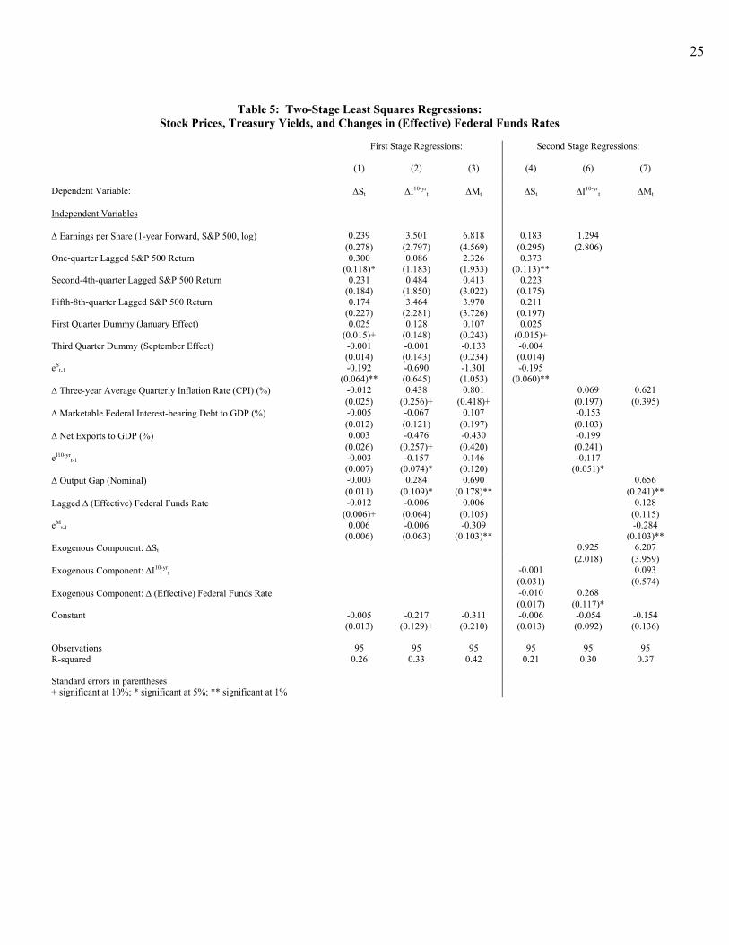
3.2. Econometric Results: The Federal Funds Rate

Table 5 presents the 2SLS regressions using the effective federal funds rate as the proxy

for Mt. Models 1, 2, and 3 are the first stage regressions, and Models 4, 5, and 6 are the second

stage regressions for ∆St, ∆I10-yrt, and ∆Mt, respectively. Two sets of questions are relevant.

16 Results that do not include eM

t-1 are available on request.

15

First, how well do the instruments perform in the first stage regressions? And, second, given the

instruments, are the exogenous components of ∆St, ∆I10-yrt, and ∆Mt statistically significant?

Regarding the first question, Model 1, the first stage regression for ∆St, indicates that

one-quarter lagged return is statistically significant and positive, consistent with Harasty and

Roulet (2000) but in contrast to the short-run contrarian hypothesis (Jegadeesh, 1990). Also, the

dummy variable for the first quarter is statistically significant, at least with 10 percent

confidence, broadly consistent with the January effect. Finally, the error correction term, eSt-1 is

safely statistically significant and suggests that about 19.2 percent of the disequilibrium in the

long-run relation is corrected each quarter. None of the other variables that purportedly help

identify short-run movements in stock prices are statistically significant, and the exogenous

variables together explain about 0.26 percent of the variance in ∆St.

The first stage regression for ∆I10-yrt, Model 2, indicates that ∆πe

t is positive as expected

and statistically significant, albeit with 10 percent confidence. Also, consistent with the

cointegrating regression, ∆NXt is negative and significant with 10 percent confidence, and eI10-yrt-

1 is statistically significant and indicates that approximately 15.7 percent of the disequilibrium is

corrected each quarter. The R2 for the first stage regression for ∆I10-yrt is 0.33.

Model 3, the first stage regression for ∆Mt, indicates that ∆πet and ∆ψt are statistically

significant with the expected positive signs, and eMt-1, which is safely statistically significant,

suggests that about 30.9 percent of the Taylor Rule disequilibrium is corrected each quarter. The

exogenous variables explain about 42 percent of the variance in ∆Mt.

With respect to the second question, Model 4 is the second stage regression for ∆St and

follows (6) but with the exogenous components for ∆I10-yrt and ∆Mt. Although the exogenous

components for ∆I10-yrt and ∆Mt have the expected negative signs, the estimates are not

16

statistically significant. Therefore, the system of equations suggests that changes in the stance of

monetary policy and changes in interest rates do not affect stock returns, ceteris paribus. Rather,

Model 4 indicates that one-period lagged stock returns, the January (first quarter) effect, and the

error correction term are statistically significant.

Model 5, the second stage regression for ∆I10-yrt, indicates that changes in monetary

policy affect changes in interest rates – the exogenous component of ∆Mt is statistically

significant and positive, consistent with the hypothesis. The coefficient suggests that a 100 basis

point increase in the federal funds rates corresponds with an approximate 26.8 basis point

increase in 10-year Treasury yields. The estimate for ∆St is not robust, and the only other

statistically significant variable in the second stage regression is eI10-yrt-1.

Finally, the second stage regression for ∆Mt suggests that stock returns and changes in

Treasury yields do not affect changes in the stance of monetary policy. According to Model 6,

the orthogonal components of ∆St and ∆I10-yrt are not statistically significant, although the

coefficients have the expected signs. Rather, the regression suggests that ∆ψt and eMt-1 are

statistically significant with the expected signs.17

17 Results using the real effective funds rate are available on request.

17

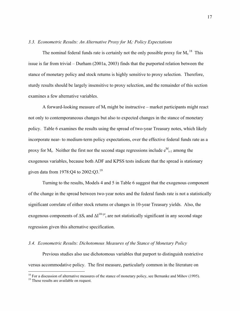
3.3. Econometric Results: An Alternative Proxy for Mt: Policy Expectations

The nominal federal funds rate is certainly not the only possible proxy for Mt.18 This

issue is far from trivial – Durham (2001a, 2003) finds that the purported relation between the

stance of monetary policy and stock returns is highly sensitive to proxy selection. Therefore,

sturdy results should be largely insensitive to proxy selection, and the remainder of this section

examines a few alternative variables.

A forward-looking measure of Mt might be instructive – market participants might react

not only to contemporaneous changes but also to expected changes in the stance of monetary

policy. Table 6 examines the results using the spread of two-year Treasury notes, which likely

incorporate near- to medium-term policy expectations, over the effective federal funds rate as a

proxy for Mt. Neither the first nor the second stage regressions include eMt-1 among the

exogenous variables, because both ADF and KPSS tests indicate that the spread is stationary

given data from 1978:Q4 to 2002:Q3.19

Turning to the results, Models 4 and 5 in Table 6 suggest that the exogenous component

of the change in the spread between two-year notes and the federal funds rate is not a statistically

significant correlate of either stock returns or changes in 10-year Treasury yields. Also, the

exogenous components of ∆St and ∆I10-yrt are not statistically significant in any second stage

regression given this alternative specification.

3.4. Econometric Results: Dichotomous Measures of the Stance of Monetary Policy

Previous studies also use dichotomous variables that purport to distinguish restrictive

versus accommodative policy. The first measure, particularly common in the literature on 18 For a discussion of alternative measures of the stance of monetary policy, see Bernanke and Mihov (1995). 19 These results are available on request.

18

monthly and quarterly stock returns, is a “tightening” dummy variable that takes a value of “1”

for a quarter if the last change in the nominal target federal funds rate was an increase and a

value of “0” if the last change was a decrease.20 Use of a dichotomous variable necessitates

some changes in the econometric esimation of the first and second stage regressions. Similar to

the models in Table 6, the exogenous variables do not include an estimate for eMt-1, and the first

and second stage equations for Mt, Models 3 and 6, are probit regressions.

The results in Table 7 using the tightening dummy variable suggest that the stance of

monetary policy does not affect asset prices. While Models 4 and 5 produce coefficients that

have the expected sign, the exogenous component of the tightening dummy is not robust in the

second stages regressions for ∆St and ∆I10-yrt.

This alternative specification, however, suggests that monetary policy responds to

changes in Treasury yields. Model 6 suggests that tightening episodes are more likely when the

exogenous component of Treasury yields increases. Similar to the results in Tables 5 and 6, the

orthogonal component of ∆St is not robust in the second stages regressions for ∆I10-yrt or Mt.

The tightening dummy variable is somewhat peculiar in that the level of Mt enters the

short-run regressions. This is, however, consistent with many studies that test whether stock

returns are lower (higher) during tightening (easing) episodes, regardless of the stage of the

monetary policy cycle. But to the contrary, perhaps initial changes in the prevailing monetary

policy regime are critical, as the first move in either a tightening or easing cycle possibly has a

pronounced impact on asset prices.

20 Despite its diminutive status as a policy tool, several studies of the effect of monetary policy on monthly and quarterly stock returns, such as Jensen and Johnson (1995) and Conover et al. (1999a, 1999b), use the discount rate, while Durham (2003) uses the federal funds rate. Given data limitations, the target federal funds discount rate tightening dummy uses the discount rate before 1986.

19

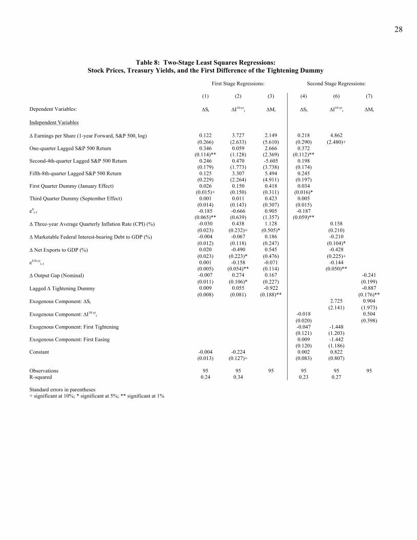
To test this notion, Table 8 reports the results using the first difference of the tightening

dummy as the proxy for Mt. Notably, the first difference of the dichotomous variable has three

possible values – a change from easing to tightening, a change from tightening to easing, or no

change in prevailing policy. Therefore, the first and second stage regressions for ∆Mt, Models 3

and 6, are multinomial probit models.

These data suggest that initial changes in the monetary policy regime also do not affect

asset prices. The exogenous components of the first tightening and first easing dummy variables

have the expected signs in the second stage model for ∆St (Model 4, Table 8), but the estimates

are not statistically significant. Also, the exogenous component of the first tightening dummy

variable is perversely signed in the second stage regression for ∆I10-yrt (Model 5), and both

estimates are statistically insignificant. Finally, the exogenous components of ∆St and ∆I10-yrt are

not statistically significant in any second stage regressions given this alternative specification.21

4. Conclusions

The preceding analyses address the existing literature on the effects of monetary policy

on asset prices in two general ways. First, the estimates follow a simple error correction

specification, which is particularly useful given the posited transitory effects of monetary policy.

Second, the 2SLS regressions relax the assumption that stock prices, interest rates, and monetary

policy are exogenous in the short-run.

In general, the error correction terms are statistically significant, which therefore suggests

that the markets for equities and Treasury securities exhibit some reversion force toward

equilibrium from period to period. Indeed, each of the eight estimates of eSt-1 and eI10-yr

t-1 are

21 Results using dichotomous variables based on the real effective funds rate are available on request.

20

statistically significant in both the first and second stage regressions in Tables 5-8. However,

this inference ultimately rests on the fine distinction between I(1) processes and stationary series

with parameter break(s).

In general, these results using data from 1978:Q4 to 2002:Q3 indicate that monetary

policy has limited impact on financial asset prices at a quarterly frequency.22 The exception is

the finding that the exogenous component of the nominal federal funds rate is a statistically

significant determinant of 10-year Treasury yields, ceteris paribus. In addition, few data suggest

that monetary policy responds to changes in asset prices, although the coefficient for the

exogenous component of ∆I10-yrt is significant in the second stage probit model of the tightening

dummy variable.

Additional research would be instructive. For example, with respect to both cointegration

theory and simultaneous equation estimation, perhaps alternative econometric techniques would

be useful. In addition, while data are somewhat limited, especially in the context of error

correction methodology, consideration of how the effect of monetary policy on asset prices

changes over time would be useful. Indeed, changes in Federal Reserve disclosure policy,

particularly since 1994, have perhaps influenced how market participants react to news and

expectations about monetary policy. But nonetheless, any possible estimations of the relations

between monetary policy on asset prices should directly address the issue of simultaneity.

22 Use of high frequency data arguably ameliorates the issue of simultaneity bias. In the very short run, perhaps monetary policy announcements are truly exogenous shocks to asset prices, at least for the immediate period bracketing the news about policy. But use of short-run data is somewhat limited in the context of monetary policy transmission, which purportedly works with sufficiently long lags – the initial policy reaction, however exogenous, might unwind or, simply, other market forces might dwarf the effect of policy over longer periods.

21

Table 1: Unit Root and Mean Stationarity Tests, Stock Market Equations*

Variable Test p value ηu Lags Obs.

S&P 500 (Log) ADF 0.593 8 96

KPSS 1.133 8 96

ADF 0.711 1 96

KPSS 4.748 1 96

∆S&P 500 (Log) ADF 0.809 8 96

KPSS 0.146 8 96

ADF 0.000 1 96

KPSS 0.190 1 96

Earnings per Share (1-year Forward, S&P 500, log) ADF 0.920 8 88

KPSS 1.144 8 96

ADF 0.740 1 95

KPSS 4.752 1 96

∆ Earnings per Share (1-year Forward, S&P 500, log) ADF 0.011 8 87

KPSS 0.076 8 96

ADF 0.001 1 94

KPSS 0.129 1 96

10-year Treasury Yield ADF 0.843 8 96

KPSS 0.984 8 96

ADF 0.713 1 96

KPSS 3.868 1 96

∆10-year Treasury Yield ADF 0.010 8 96

KPSS 0.147 8 96

ADF 0.000 1 96

KPSS 0.138 1 96

eSt ADF 0.037 8 87

KPSS 0.061 8 96

ADF 0.079 1 94

KPSS 0.154 1 96 *KPSS critical values of ηu for H0 of level stationarity are 0.347 (10 percent), 0.463 (5 percent), and 0.739 (1 percent).

22

Table 2: Unit Root and Mean Stationarity Tests: Treasury Yield Equations*

Variable Test p value ηu Lags Obs.

Three-year Average Quarterly Inflation Rate (CPI) (%) ADF 0.657 8 96

KPSS 0.753 8 96

ADF 0.441 1 96

KPSS 3.088 1 96

∆ Three-year Average Quarterly Inflation Rate (CPI) (%) ADF 0.001 8 96

KPSS 0.072 8 96

ADF 0.021 1 96

KPSS 0.211 1 96

Real (Effective) Federal Funds Rate ADF 0.131 8 96

KPSS 0.261 8 96

ADF 0.026 1 96

KPSS 0.744 1 96

∆ Real (Effective) Federal Funds Rate ADF 0.010 8 96

KPSS 0.177 8 96

ADF 0.000 1 96

KPSS 0.092 1 96

Marketable Federal Interest-bearing Debt to GDP (%) ADF 0.180 8 96

KPSS 0.644 8 96

ADF 0.411 1 96

KPSS 2.665 1 96

∆ Marketable Federal Interest-bearing Debt to GDP (%) ADF 0.289 8 96

KPSS 0.530 8 96

ADF 0.017 1 96

KPSS 1.729 1 96

Net Exports to GDP (%) ADF 0.501 8 96

KPSS 0.445 8 96

ADF 0.872 1 96

KPSS 1.673 1 96

∆ Net Exports to GDP (%) ADF 0.104 8 96

KPSS 0.139 8 96

ADF 0.000 1 96

KPSS 0.172 1 96

eI10-yrt ADF 0.064 8 87

KPSS 0.093 8 96

ADF 0.016 1 94

KPSS 0.186 1 96 *KPSS critical values of ηu for H0 of level stationarity are 0.347 (10 percent), 0.463 (5 percent), and 0.739 (1 percent).

23

Table 3: Unit Root and Mean Stationarity Tests: Taylor Rule Equations* Variable Test p value ηu Lags Obs.

(Effective) Federal Funds Rate ADF 0.610 8 96

KPSS 0.880 8 96

ADF 0.548 1 96

KPSS 3.273 1 96

∆ (Effective) Federal Funds Rate ADF 0.033 8 96

KPSS 0.094 8 96

ADF 0.000 1 96

KPSS 0.085 1 96

Output Gap (Nominal) ADF 0.191 8 96

KPSS 0.282 8 96

ADF 0.113 1 96

KPSS 0.930 1 96

∆ Output Gap (Nominal) ADF 0.027 8 96

KPSS 0.088 8 96

ADF 0.000 1 96

KPSS 0.125 1 96

eMt ADF 0.573 8 87

KPSS 0.266 8 96

ADF 0.034 1 94

KPSS 0.780 1 96 *KPSS critical values of ηu for H0 of level stationarity are 0.347 (10 percent), 0.463 (5 percent), and 0.739 (1 percent).

24

Table 4: Cointegrating Regressions

Stock Prices, Treasury Yields, and the Effective Federal Funds Rate (1) (2) (3) Dependent Variable: St I10-yr

t Mt Independent Variables Earnings per Share (1-year Forward, S&P 500, log) 1.477 -2.648 (0.044)** (0.400)** 10-year Treasury Yield -0.065 (0.008)** Three-year Average Quarterly Inflation Rate (CPI) (%) 0.884 1.399 (0.142)** (0.070)** Marketable Federal Interest-bearing Debt to GDP (%) 0.113 (0.042)** Net Exports to GDP (%) -0.903 (0.233)** Output Gap (Nominal) 0.686 (0.086)** Constant 1.466 7.757 1.595 (0.202)** (2.742)** (0.321)** Observations 96 96 96 R-squared 0.98 0.80 0.82 Standard errors in parentheses + significant at 10%; * significant at 5%; ** significant at 1%

25

Table 5: Two-Stage Least Squares Regressions:

Stock Prices, Treasury Yields, and Changes in (Effective) Federal Funds Rates First Stage Regressions: Second Stage Regressions: (1) (2) (3) (4) (6) (7) Dependent Variable: ∆St ∆I10-yr

t ∆Mt ∆St ∆I10-yrt ∆Mt

Independent Variables ∆ Earnings per Share (1-year Forward, S&P 500, log) 0.239 3.501 6.818 0.183 1.294 (0.278) (2.797) (4.569) (0.295) (2.806) One-quarter Lagged S&P 500 Return 0.300 0.086 2.326 0.373 (0.118)* (1.183) (1.933) (0.113)** Second-4th-quarter Lagged S&P 500 Return 0.231 0.484 0.413 0.223 (0.184) (1.850) (3.022) (0.175) Fifth-8th-quarter Lagged S&P 500 Return 0.174 3.464 3.970 0.211 (0.227) (2.281) (3.726) (0.197) First Quarter Dummy (January Effect) 0.025 0.128 0.107 0.025 (0.015)+ (0.148) (0.243) (0.015)+ Third Quarter Dummy (September Effect) -0.001 -0.001 -0.133 -0.004 (0.014) (0.143) (0.234) (0.014) eS

t-1 -0.192 -0.690 -1.301 -0.195 (0.064)** (0.645) (1.053) (0.060)** ∆ Three-year Average Quarterly Inflation Rate (CPI) (%) -0.012 0.438 0.801 0.069 0.621 (0.025) (0.256)+ (0.418)+ (0.197) (0.395) ∆ Marketable Federal Interest-bearing Debt to GDP (%) -0.005 -0.067 0.107 -0.153 (0.012) (0.121) (0.197) (0.103) ∆ Net Exports to GDP (%) 0.003 -0.476 -0.430 -0.199 (0.026) (0.257)+ (0.420) (0.241) eI10-yr

t-1 -0.003 -0.157 0.146 -0.117 (0.007) (0.074)* (0.120) (0.051)* ∆ Output Gap (Nominal) -0.003 0.284 0.690 0.656 (0.011) (0.109)* (0.178)** (0.241)** Lagged ∆ (Effective) Federal Funds Rate -0.012 -0.006 0.006 0.128 (0.006)+ (0.064) (0.105) (0.115) eM

t-1 0.006 -0.006 -0.309 -0.284 (0.006) (0.063) (0.103)** (0.103)** Exogenous Component: ∆St 0.925 6.207 (2.018) (3.959) Exogenous Component: ∆I10-yr

t -0.001 0.093 (0.031) (0.574) Exogenous Component: ∆ (Effective) Federal Funds Rate -0.010 0.268 (0.017) (0.117)* Constant -0.005 -0.217 -0.311 -0.006 -0.054 -0.154 (0.013) (0.129)+ (0.210) (0.013) (0.092) (0.136) Observations 95 95 95 95 95 95 R-squared 0.26 0.33 0.42 0.21 0.30 0.37 Standard errors in parentheses + significant at 10%; * significant at 5%; ** significant at 1%

26

Table 6: Two-Stage Least Squares Regressions:

Stock Prices, Treasury Yields, and Changes in 2-Year Treasury Spread over Federal Funds Rates First Stage Regressions: Second Stage Regressions: (1) (2) (3) (4) (6) (7) Dependent Variable: ∆St ∆I10-yr

t ∆Mt ∆St ∆I10-yrt ∆Mt

Independent Variables ∆ Earnings per Share (1-year Forward, S&P 500, log) 0.065 3.147 -3.104 0.109 2.806 (0.267) (2.612) (3.333) (0.301) (2.805) One-quarter Lagged S&P 500 Return 0.357 0.226 -1.238 0.358 (0.115)** (1.127) (1.439) (0.114)** Second-4th-quarter Lagged S&P 500 Return 0.247 0.601 1.484 0.234 (0.181) (1.766) (2.254) (0.179) Fifth-8th-quarter Lagged S&P 500 Return 0.148 3.447 1.432 0.216 (0.229) (2.240) (2.859) (0.201) First Quarter Dummy (January Effect) 0.024 0.154 0.019 0.025 (0.015) (0.147) (0.187) (0.015) Third Quarter Dummy (September Effect) -0.000 0.010 0.119 -0.002 (0.014) (0.142) (0.181) (0.015) eS

t-1 -0.194 -0.772 0.139 -0.187 (0.065)** (0.637) (0.813) (0.059)** ∆ Three-year Average Quarterly Inflation Rate (CPI) (%) -0.028 0.485 -0.478 0.073 -0.505 (0.024) (0.234)* (0.299) (0.212) (0.295)+ ∆ Marketable Federal Interest-bearing Debt to GDP (%) -0.005 -0.067 -0.095 -0.245 (0.012) (0.117) (0.150) (0.104)* ∆ Net Exports to GDP (%) 0.022 -0.468 0.185 -0.339 (0.023) (0.222)* (0.283) (0.239) eI10-yr

t-1 0.001 -0.163 -0.080 -0.170 (0.005) (0.053)** (0.067) (0.054)** ∆ Output Gap (Nominal) -0.005 0.305 -0.175 -0.257 (0.011) (0.106)** (0.136) (0.160) Lagged ∆ 2-year Treasury minus Federal Funds Rate 0.006 0.108 -0.222 -0.252 (0.009) (0.087) (0.111)* (0.111)* Exogenous Component: ∆St 1.942 -1.719 (2.183) (2.587) Exogenous Component: ∆I10-yr

t -0.013 0.164 (0.020) (0.297) Exogenous Component: ∆ 2-year Treasury minus Federal Funds Rate 0.002 -0.392 (0.030) (0.303) Constant -0.002 -0.224 -0.034 -0.005 -0.114 0.026 (0.013) (0.125)+ (0.160) (0.013) (0.093) (0.095) Observations 95 95 95 95 95 95 R-squared 0.23 0.34 0.14 0.21 0.27 0.08 Standard errors in parentheses + significant at 10%; * significant at 5%; ** significant at 1%

27

Table 7: Two-Stage Least Squares Regressions:

Stock Prices, Treasury Yields, and the Monetary Policy Tightening Dummy First Stage Regressions: Second Stage Regressions: (1) (2) (3) (4) (6) (7) Dependent Variable: ∆St ∆I10-yr

t Mt ∆St ∆I10-yrt Mt

Independent Variables ∆ Earnings per Share (1-year Forward, S&P 500, log) 0.193 3.450 65.898 0.447 0.749 (0.288) (2.856) (25.116)** (0.372) (3.622) One-quarter Lagged S&P 500 Return 0.346 0.079 2.624 0.360 (0.114)** (1.132) (5.137) (0.110)** Second-4th-quarter Lagged S&P 500 Return 0.229 0.421 -11.102 0.207 (0.180) (1.778) (9.084) (0.174) Fifth-8th-quarter Lagged S&P 500 Return 0.152 3.442 37.578 0.360 (0.228) (2.262) (18.331)* (0.222) First Quarter Dummy (January Effect) 0.024 0.128 0.349 0.025 (0.015) (0.147) (0.719) (0.015) Third Quarter Dummy (September Effect) 0.000 -0.002 -1.405 -0.006 (0.014) (0.143) (0.910) (0.014) eS

t-1 -0.184 -0.698 -3.412 -0.196 (0.065)** (0.643) (4.410) (0.059)** ∆ Three-year Average Quarterly Inflation Rate (CPI) (%) -0.026 0.429 3.117 0.050 -0.638 (0.024) (0.237)+ (2.405) (0.212) (0.839) ∆ Marketable Federal Interest-bearing Debt to GDP (%) -0.009 -0.068 -0.220 -0.119 (0.013) (0.125) (0.834) (0.121) ∆ Net Exports to GDP (%) 0.021 -0.481 -3.666 -0.331 (0.023) (0.224)* (1.945)+ (0.234) eI10-yr

t-1 0.002 -0.163 -0.591 -0.152 (0.006) (0.057)** (0.405) (0.050)** ∆ Output Gap (Nominal) -0.008 0.281 1.532 -0.206 (0.011) (0.107)* (0.980) (0.435) Lagged Tightening Dummy -0.015 0.007 4.068 2.790 (0.016) (0.157) (1.463)** (0.534)** Exogenous Component: ∆St 2.415 2.099 (2.110) (6.780) Exogenous Component: ∆I10-yr

t 0.001 3.514 (0.024) (1.007)** Exogenous Component: Tightening Dummy -0.004 0.043 (0.003) (0.029) Constant 0.003 -0.217 -4.227 -0.016 -0.064 -1.628 (0.014) (0.135) (1.379)** (0.015) (0.104) (0.417)** Observations 95 95 95 95 95 95 R-squared 0.23 0.33 0.23 0.27 Standard errors in parentheses + significant at 10%; * significant at 5%; ** significant at 1%

28

Table 8: Two-Stage Least Squares Regressions:

Stock Prices, Treasury Yields, and the First Difference of the Tightening Dummy First Stage Regressions: Second Stage Regressions: (1) (2) (3) (4) (6) (7) Dependent Variables: ∆St ∆I10-yr

t ∆Mt ∆St ∆I10-yrt ∆Mt

Independent Variables ∆ Earnings per Share (1-year Forward, S&P 500, log) 0.122 3.727 2.149 0.218 4.862 (0.266) (2.633) (5.610) (0.290) (2.480)+ One-quarter Lagged S&P 500 Return 0.346 0.059 2.666 0.372 (0.114)** (1.128) (2.369) (0.112)** Second-4th-quarter Lagged S&P 500 Return 0.246 0.470 -5.605 0.198 (0.179) (1.773) (3.738) (0.174) Fifth-8th-quarter Lagged S&P 500 Return 0.125 3.307 5.494 0.245 (0.229) (2.264) (4.911) (0.197) First Quarter Dummy (January Effect) 0.026 0.150 0.418 0.034 (0.015)+ (0.150) (0.311) (0.016)* Third Quarter Dummy (September Effect) 0.001 0.011 0.423 0.005 (0.014) (0.143) (0.307) (0.015) eS

t-1 -0.185 -0.666 0.905 -0.187 (0.065)** (0.639) (1.357) (0.059)** ∆ Three-year Average Quarterly Inflation Rate (CPI) (%) -0.030 0.438 1.128 0.158 (0.023) (0.232)+ (0.505)* (0.210) ∆ Marketable Federal Interest-bearing Debt to GDP (%) -0.004 -0.067 0.186 -0.210 (0.012) (0.118) (0.247) (0.104)* ∆ Net Exports to GDP (%) 0.020 -0.490 0.545 -0.428 (0.023) (0.223)* (0.476) (0.225)+ eI10-yr

t-1 0.001 -0.158 -0.071 -0.144 (0.005) (0.054)** (0.114) (0.050)** ∆ Output Gap (Nominal) -0.007 0.274 0.167 -0.241 (0.011) (0.106)* (0.227) (0.199) Lagged ∆ Tightening Dummy 0.009 0.055 -0.922 -0.887 (0.008) (0.081) (0.188)** (0.176)** Exogenous Component: ∆St 2.725 0.904 (2.141) (1.973) Exogenous Component: ∆I10-yr

t -0.018 0.504 (0.020) (0.398) Exogenous Component: First Tightening -0.047 -1.448 (0.121) (1.203) Exogenous Component: First Easing 0.009 -1.442 (0.120) (1.186) Constant -0.004 -0.224 0.002 0.822 (0.013) (0.127)+ (0.083) (0.807) Observations 95 95 95 95 95 95 R-squared 0.24 0.34 0.23 0.27 Standard errors in parentheses + significant at 10%; * significant at 5%; ** significant at 1%

29

References Bernanke, Ben S. and Ilian Mihov, 1995, “Measuring Monetary Policy,” NBER Working Paper Series No. 5145. Campbell, John Y. and P. Perron, 1991, “Pitfalls and Opportunities: What Macro-economists Should Know about Unit Roots,” in O. J. Blanchard and S. Fischer, eds., NBER Macroeconomics Annual, 1991, Cambridge MA: MIT Press, 141-200. Campbell, John Y. and Robert J. Shiller, 1987, “Cointegration and Tests of Present Value Models,” Journal of Political Economy, vol. 95, 1062-1088. Conover, C. Mitchell, Gerald R. Jensen, and Robert R. Johnson, 1999a, “Monetary Environments and International Stock Returns,” Journal of Banking and Finance, vol. 23, 1357-1381. Conover, C. Mitchell, Gerald R. Jensen, and Robert R. Johnson, 1999b, “Monetary Conditions and International Investing,” Financial Analysts Journal, 1357-1381. Cook, Timothy, and Thomas Hahn, 1988, “The Information Content of Discount Rate Annoucements and Their Effect on Market Interest Rates,” Journal of Money, Credit, and Banking, vol. 20 no. 2 (May), 167-180. De Bondt, W. R. M., and R. Thaler, 1985, “Does the Stock Market Overreact?” Journal of Finance 40, 793-805. Durham, J. Benson, 2003, “Should Equity Investors ‘Fight the Central Bank’?: The Effect of Monetary Policy on Stock Market Returns,” Financial Analysts Journal, forthcoming. Durham, J. Benson, 2001a, “The Effect of Monetary Policy on Monthly and Quarterly Stock Market Returns: Cross-Country Evidence and Sensitivity Analyses,” Finance and Economic Discussion Papers Series No. 42, Federal Reserve Board. Durham, J. Benson, 2001b, “Sensitivity Analyses of Anomalies in Developed Stock Markets,” Journal of Banking and Finance, vol. 25 (August 2001), pp. 1503-1541. Engle, R. F. and C.W.J. Granger, 1987, “Cointegration and Error Correction: Representation, Estimation and Testing,” Econometrica, vol. 55, pp. 251-276. Granger, Clive W. J., 1986, “Developments in the Study of Cointegrated Economic Variables,” Oxford Bulletin of Economics and Statistics, vol. 48 no. 3, 213-228. Harasty, Hélène, and Jacques Roulet, 2000, “Modeling Stock Market Returns: An Error Correction Model,” Journal of Portfolio Management, vol. 26 no. 2 (Winter), 33-46.

30

Haugen, R. A. and Lakonishok, 1987, The Incredible January Effect (Irwin: Homewood, Illinois). Howe, Howard and Charles Pigott, 1991-1992, “Determinants of Long-Term Interest Rates: An Empirical Study of Several Industrial Countries,” Federal Reserve Bank of New York Quarterly Review, (Winter), 12-28. Jegadeesh, N., 1990, “Evidence of Predictable Behavior of Security Returns,” Journal of Finance, vol. 45, 881-98. Jensen, Gerald R. and Robert R. Johnson, 1995, “Discount Rate Changes and Security Returns in the U.S., 1962-1991,” Journal of Banking and Finance, vol. 19, 79-95. Jensen, Gerald R., Jeffry M. Mercer, and Robert R. Johnson, 1996, “Business Conditions, Monetary Policy, and Expected Security Returns,” Journal of Financial Economics, vol. 40, 213-237. Johansen, S., 1988, “Statistical Analysis of Cointegrating Vectors,” Journal of Economic Dynamics and Control, vol. 12, 1-14. Johansen, S. and K. Juselius, “Maximum-Likelihood Estimation and Inference on Cointegration – With Applications to the Demand for Money,” Oxford Bulletin of Economics and Statistics, vol 52, 169-210. Kwiatkowski, Dennis, Peter C. B. Phillips, Peter Schmidt, and Yoncheol Shin, 1992, “Testing the Null Hypothesis of Stationarity Against the Alternative of a Unit Root: How Sure Are We that Economic Time Series have a Unit Root?” Journal of Econometrics, vol. 54 (October-December), 159-178. Mehra, Yash P., 1994, “An Error-Correction Model of the Long-Term Bond Rate,” Federal Reserve Bank of Richmond Economic Quarterly, vol. 80, no. 4 (Fall), 49-68. Perron, Pierre, 1989, “The Great Crash, the Oil Price Shock, and the Unit Root Hypothesis,” Econometrica, vol. 57 no. 6 (November), 1361-1401. Perron, Pierre, 1997, “Further Evidence on Breaking Trend Functions in Macroeconomic Variables,” Journal of Econometrics, vol. 80, 355-385. Sargent, Thomas J., 1969, “Commodity Price Expectations and the Interest Rate,” Quarterly Journal of Economics, vol. 83 (February), 127-140. Siegel, Jeremy, 1998, Stocks for the Long-Run: The Definitive Guide to Financial Market Returns and Long-Term Investment Strategies (New York: McGraw-Hill). Smirlock, Michael and Jess Yawitz, 1985, “Asset Returns, Discount Rate Changes, and Market Efficiency,” Journal of Finance, vol. 40 no. 4 (September), 1141-1158.

31

Taylor, John, 1993, “Discretion versus Policy Rules in Practice,” Carnegie-Rochester Conference Series on Public Policy, vol. 39, 195-214. Waud, R., 1970, “Public Interpretation of Federal Reserve Discount Rate Changes: Evidence on the ‘Announcement Effect,’” Econometrica, vol. 38, 231-250.