Does Money Illusion Matter?

An Experimental Approach

ERNST FEHR1 and JEAN-ROBERT TYRAN2

First Version: October 1997

This Version: February 1998

Abstract

Money illusion means that people behave differently when the same objectivesituation is represented in nominal or in real terms. To examine the behavioralimpact of money illusion we studied the adjustment process of nominal prices aftera fully anticipated negative nominal shock in an experimental setting with strategiccomplementarity. We show that seemingly innocuous differences in payoff presen-tation cause large behavioral differences. In particular, if the payoff information ispresented to subjects in nominal terms, price stickiness and real effects are muchmore pronounced than when payoff information is presented in real terms. The dri-ving force of differences in real outcomes is subjects’ expectation of higher nominalinertia in the nominal payoff condition. Due to strategic complementarity, theseexpectations induce subjects to adjust rather slowly to the shock.

Keywords: Money illusion, nominal inertia, sticky prices, non-neutrality of money

JEL: C92, E32, E52.

1. University of Zürich, Institute for Empirical Research in Economics, Blümlisalpstr. 10, CH-8006 Zürich. E-Mail address: efehr@iew.unizh.ch

2. University of St. Gallen, Department of Economics, Bodanstr. 1, CH-9000 St. Gallen. E-Mailaddress: Jean-Robert.Tyran@vwa.unisg.chWe are particularly grateful for comments by George Akerlof, Jim Cox, Urs Fischbacher, SimonGächter, Linda Babcock, and Dick Thaler. In addition, we acknowledge helpful comments by theparticipants of Seminars at Bonn, Mannheim, the NBER conference on behavioral macroeconomicsand the Amsterdam workshop for experimental economics. Valuable research assistance has beenprovided by Martin Brown, Beatrice Zanella and Tobias Schneider. We are grateful for financialsupport by the Swiss National Science Foundation under project no. 1214-051000.97/1

2

1. Introduction

The notion of money illusion seems to be thorougly discredited in modern economics. Tobin

(1972), for example, described the negative attitude of most economic theorists towards money

illusion as follows: “An economic theorist can, of course, commit no greater crime than to assume

money illusion.“ As a consequence, money illusion is anathema in the profession. For example,

that the Index of the Handbook of Monetary Economics (Friedman and Hahn 1990) does not even

mention the term “money illusion“. In principle, money illusion could provide an explanation for

the inertia of nominal prices and wages and, thus, for the non-neutrality of money. The stickiness

of nominal prices and wages seems to be an important phenomenon (see e.g. Akerlof, Dickens and

Perry 1996, Bernanke and Carey 1996, Kahn 1996) and has puzzled economists for decades

because it is quite difficult to explain in an equilibrium model with maximizing individuals.

Instead of money illusion other factors like informational frictions (Lucas 1972), staggering of

contracts (e.g., Fischer 1977, Taylor 1979), costs of price adjustment (Mankiw 1985) and near-

rationality (Akerlof and Yellen 1985) have been invoked to explain nominal inertia.

In this paper we do not contest the potential relevance of these explanations. We do, however,

argue that money illusion has been dismissed prematurely as a potential candidate for the explana-

tion of sluggish nominal price adjustment. Our argument is based on theoretical considerations

and on experimental evidence. At the theoretical level we will argue that in order to rule out the

relevance of money illusion it is not sufficient that individuals are illusion-free but that the

absence of money illusion is common knowledge. Yet, in our view, it seems highly unlikely that

this common knowledge requirement is met in practice. At the empirical level we will show that,

after a fully anticipated negative nominal shock, nominal inertia is the rule rather than the excep-

tion. Substantial nominal inertia arises even if informational frictions, costs of price adjustment

and staggering are absent.

Money illusion means that behavior depends on whether the same objective situation is framed

in nominal or in real terms. A particularly transparent example of money illusion is the case where

people behave differently when they receive payoff information in real or in nominal terms. In

fact, almost all business transactions involve nominal payoff information. To detect this kind of

money illusion it would, thus, be necessary to find situations in which a real frame, e.g., only real

payoff information, prevails. By comparing people’s behavior under the nominal and the real

frame one could isolate the behavioral impact of money illusion. Unfortunately, business life does

not seem to provide examples in which the same objective situation is sometimes represented in

3

nominal terms and sometimes in real terms. This is one important reason why we rely in our empi-

rical examination on experimental methods.3 In the present context a major advantage of experi-

mental methods is that the “frame“ is under the control of the experimenter. Accordingly, we

implemented a treatment condition in which payoffs were represented in nominal terms and a con-

trol condition in which payoffs were represented in real terms. It turns out that this seemingly

innocuous difference in payoff presentation causes large differences in behavior. In particular,

nominal inertia is much more pronounced in the nominal payoff condition. This behavioral diffe-

rence occurs although subjects in the nominal condition have been trained how to compute real

payoffs from the nominally given payoffs. Under the nominal payoff representation it takes roug-

hly twice as long for the economy to reach the “new“4, post-shock-equilibrium. In addition, real

income losses are approximately twice as large in the nominal condition. This indicates that the

“veil of money“, that is, the veil generated by the nominal representation of payoffs, has beha-

vioral effects with large real consequences after an anticipated nominal shock.

The major cause for the slow price adjustment is the inertia of subjects’ expectations about the

prices set by others. In all experimental conditions subjects do not expect that the other subjects

immediately jump to the ‘new’ equilibrium. Therefore, subjects do, in general, have no incentive

to play the post-shock equilibrium immediately after the shock. Moreover, and perhaps more

importantly, the stickiness of price expectations is much larger in the nominal payoff condition.

Thus subjects expect much less adjustment by others in this condition after the shock. These diffe-

rences in expectations suggest that money illusion matters because the absence of money illusion

is not common knowledge and less so, because subjects themselves cannot pierce the veil of

money.

The rest of the paper is organized in the following way. In section 2 we discuss the notion of

money illusion and its potential aggregate implications in more detail. In section 3 we argue that

experimental methods are an appropriate tool for the study of money illusion and outline our expe-

rimental design. In section 4 the experimental results are presented. In the final section we summa-

rize and interpret our main results.

3. Section 3 provides further reasons for the application of experimental methods to the problem of money illu-sion.

4. In fact, it is the same equilibrium in real terms.

4

2. Money illusion, disequilibrium and strategic complementarity

2.1. Money illusion at the individual level

The term “money illusion“ has been used differently by various authors although the intuition

on which the term is based seems to be rather similar.5 Leontief (1936), for example, defined

money illusion as a violation of the “homogeneity postulate“. This postulate stipulates that

demand and supply functions are homogeneous of degree zero in all nominal prices, i. e., they

depend only on relative and not on absolute prices. Patinkin (1949) used a slightly different defini-

tion that also takes into account the potential effect of people’s real wealth on their supply and

demand behavior. According to Patinkin money illusion is absent if individuals’ net demand

functions are homogeneous of degree zero in all money prices and real wealth.

Although the definition of Patinkin differs from Leontief’s by taking into account the “wealth

constraint“, both definitions are, in our view, based on the same intuition. This intuition says that if

the real incentive structure, i.e. the objective situation an individual faces, remains unchanged, the

real decisions of an illusion-free individual do not change either. Two crucial assumptions underly

this intuition: First, the objective function of the individual does not depend on nominal but only

on real magnitudes. Second, people perceive that purely nominal changes do not affect their

opportunity set. For example, people have to understand that an equiproportionate change in all

nominal magnitudes leaves the real constraints unaffected. Whether people are indeed able to

pierce the veil of money and to understand that purely nominal changes leave their objective cir-

cumstances unchanged is, in principle, an empirical question. Irving Fisher (1928: 4), for example,

was convinced that ordinary people, in general, fail “to perceive that the dollar, or any other unit of

money expands or shrinks in value“ after a monetary shock.

More recently Shafir, Tversky and Diamond (henceforth STD, 1997) provided evidence that

indicates that frequently one or both preconditions for the absence of money illusion are violated.

Their results suggest that people’s preferences as well as their perceptions of the constraints are

affected by nominal values. Moreover, many people do not only seem to suffer from money illu-

sion; they also expect that other people’s preferences and decisions are affected by money illusion.

Problem 1 of STD’s questionnaire study neatly illustrates these claims. STD presented the follo-

wing scenario to two groups of respondents:

5. For the different definitions of money illusion see Howitt (1989).

5

Consider two individuals, Ann and Barbara, who graduated from the same college a year apart. Upon graduation, both took similar jobs with publishing firms. Ann started with a yearly salary of $ 30,000. During her first year on the job there was no infla-tion, and in her second year Ann received a 2% ($ 600) raise in salary. Barbara also started with a yearly salary of $ 30,000. During her first year on the job there was a 4 % inflation, and in her second year Barbara received a 5% ($ 1500) raise in salary.

Respondents of group 1 were then asked the happiness question: “As Ann and Barbara entered

their second year on the job, who do you think was happier?“ 36 percent thought that Ann was

happier while 64 percent believed that Barbara was happier. This indicates that most subjects

believed that preferences are affected by nominal variables because in real terms Ann does of

course better.6 Respondents of group 2 were asked the following question: “As they entered their

second year on the job, each received a job offer from another firm. Who do you think was more

likely to leave the present position for another job?“ In line with the response to the happiness

question 65 percent believed that Ann, which is doing better in economic terms, is more likely to

leave the present job. Thus, a majority believed that other people’s decisions are affected by

money illusion.

Since the absence of money illusion means that an individual’s preferences, perceptions and,

hence, choices of real magnitudes are not affected by purely nominal changes it is natural to view

money illusion as a framing or representation effect. From this viewpoint an individual exhibits

money illusion if the preferences or the perceptions of constraints and the associated decisions

depend on whether the same environment is represented in nominal or real terms. STD’s analysis

is based on a large body of research in cognitive psychology that shows that alternative representa-

tions of the same situation may well lead to systematically different responses (Tversky and Kahn-

eman 1981, 1986).7 Representation effects seem to arise because people tend to adopt the

particular frame that is presented and evaluate the options within this frame. Because some options

loom larger in one representation than in another, alternative framings of the same options can

give rise to different choices.

STD argue that people tend to have multiple representations but that the nominal representa-

tion is often simpler and more salient. They suggest that people are generally aware of the diffe-

rence between nominal and real values, but because money is a salient and natural unit, people

often think of transactions in predominantly nominal terms. Thinking in terms of relative prices

does not seem natural to many people. For example, most people tend to say “this beer has a price

6. There was a third group of respondents who was asked whether Ann or Barbara are doing better in economicterms. 71 percent answered that Ann is in fact doing better in economic terms.

7. For an early demonstration of a framing or representation effect in experimental economics see Selten andBerg (1970).

6

of 2$, and this steak a price of 7$“, but only few people would state “this steak has a price of 3.5

beers“.

2.2. Money illusion as a disequilibrating force

In the past economists frequently used the assumption of money illusion to account for the

short-run non-neutrality of money. Irving Fisher’s explanation of business cycles is, for example,

based on lenders’ money illusion during an upswing.8 However, since the success of the rational

expectations revolution an extreme reluctance to invoke money illusion as an explanation of the

short-run non-neutrality of money has been established. While New Classical macroeconomists

focus on informational frictions to account for short-run non-neutrality (Lucas 1972), New Key-

nesians mainly focus on costs of price adjustment or staggering (see e. g. Mankiw and Romer

1991).9 In the absence of menu costs, staggering, and informational frictions, the models of New

Keynesian and New Classical economists rule out that purely monetary changes have real effects.

A common feature of these models is that they exclusively focus on the equilibrium states of their

economies. In general, they remain silent on how economic agents move from one equilibrium to

the other. In models that exclusively focus on equilibrium the assumption of the absence of money

illusion is very intuitive because it is difficult to imagine that an illusion could persist in equili-

brium.

However, as we will argue next, there is a strong a priori argument that money illusion is likely

to affect the adjustment process of an economy after a fully anticipated monetary shock. Our argu-

ment is based on the simple fact that a Nash equilibrium involves the coordination of expectations.

This can be illustrated in the context of a monopolistically competitive economy as analysed in,

for example, Akerlof and Yellen (1985) or Blanchard and Kiyotaki (1987). To keep the argument

simple we focus only on firms’ behavior. The reduced form real profit function for firms in these

models can be written as

(1)

where is firm i’s real profit, is the nominal price set by firm i, is the aggregate price

level and M denotes the supply of money.10 In these models is proportional to real aggre-

8. Fisher believed that lenders are willing to supply more in the face of a rise in nominal interest rates althoughreal interest rates decline or remain unchanged due to inflation.

9. The near-rationality approach of Akerlof and Yellen (1985) can, in principle, be subsumed under the menu-costapproach by stipulating “cognitive“ menu costs of maximizing behavior.

πi πi Pi P⁄ M P⁄,( )=

πi Pi P

M P⁄

7

gate demand. For simplicity, we assume identical firms and a unique symmetric equilibrium

, for all i, j. In this equilibrium each firm maximizes its real profits by setting

. Since (1) is homogeneous of degree zero in , and M it is obvious that a change in

M to , ( ), leads to post shock equilibrium values of and .

Suppose now that there are agents who believe that there are other agents who suffer from

money illusion and do not fully adjust their nominal prices to . The first group of agents, the-

refore, anticipates a change in real aggregate demand so that their members, in general,

have an incentive to choose a price that differs from . For this conclusion to hold, it is not

even necessary that there are indeed firms which believe that others suffer from money illusion.

Suppose, for example, that there is one group of firms, which believes that a second group of firms

believes, that there is a third group which suffers from money illusion and does, hence, not adjust

fully. This means that the first group believes that the second group does not choose the equili-

brium price and, hence, the first group also has an incentive to choose a price which differs

from the equilibrium price. The basic message of this argument is, thus, that unless the absence of

money illusion is common knowledge, there will, in general be no coordinated instantaneous adju-

stment to . As a consequence, the economy will go through a process of disequilibrium.

2.3. Strategic complementarity and the aggregate impact of money illusion

Considering the evidence of STD it seems rather likely that the absence of money illusion is

not common knowledge. However, the disequilibrating force of money illusion does not per se

provide a reason for aggregate nominal inertia. It also is not clear whether the disequilibrium is

associated with economically significant welfare effects. At this point of the argument strategic

complementarity becomes important. Haltiwanger and Waldman (1989) have shown that in the

presence of strategic complementarity between agents’ decisions the existence of a small group of

nonrational subjects can have large effects on the process of adjustment to equilibrium.11 In the

above mentioned model of monopolistic competition strategic complementarity means that firm i’s

profit maximizing nominal price is positively related to the aggregate price level . This

10. Equation (1) already incorporates (i) the maximizing behavior of all households, (ii) the cost minimizing beha-vior of all firms for given output and wages levels, (iii) the equilibrium real wage, and (iv) the equilibrium rela-tion between real aggregate demand and real money balances. In Akerlof and Yellen (1985) the real wage isgiven by the Solow condition because firms are efficiency wage setters. In Blanchard and Kiyotaki (1987)housholds are wage setters so that firms take real wages as given when choosing nominal prices and output.

11. The papers by Haltiwanger and Waldman (1985) and Russell and Thaler (1985) examine a related point. Theyanalyze the conditions under which nonrational subjects affect the equilibrium. In contrast, Haltiwanger andWaldman (1989) examine the conditions under which nonrational subjects affect the adjustment to equilibrium.

Pi∗ Pj

∗=

Pi∗ P

∗= Pi P

λM λ 1≠ λPi∗ λP

∗

λPi

M P⁄

λPi∗

λPi∗

λPi∗

Pi’ P

8

means that firms which believe that other agents’ money illusion keeps close to its pre-shock

equilibrium level have a rational reason to choose a nominal price that is close to the pre-shock

equilibrium level. Likewise, firms which believe that other firms believe that there is money illu-

sion in the economy will also have a rational reason to stay close to the pre-shock price level, and

so forth.

Under strategic complementarity rational firms have an incentive to partly imitate the behavior

of the nonrational ones which gives the latter a disproportionately large impact on the aggregate

price level. In contrast, in the presence of strategic substitutability, i. e., if is negatively related

to , rational firms have an incentive to partly compensate the behavior of the nonrational ones so

that the latter have a disproportionately small impact on the aggregate. The results of Haltiwanger

and Waldmann (1989) thus suggest that, given strategic complementarity, expectations about the

existence of a small group of subjects that suffer from money illusion may generate substantial

nominal inertia.

The essence of the above argument is that a rational player has to base his choice on his fore-

cast of other players’ actions. These actions in turn depend on the forecasts of the behavior of

other players, and so on. Therefore, a rational player has to make forecasts about the forecasts of

others, etc. If at one stage in this chain of reasoning there is the belief that money illusion gives

rise to less than full adjustment, rational players have an incentive to adjust less than fully, too.

The situation is similar to Keynes’ famous “beauty contest“-analogy for professional investors.

Keynes argued that to make profit in the stock market it is crucial to know the average opinion of

the other investors which in turn depends on their estimates of the average opinion, and so on.12

Keynes argument implies that in the absence of common knowledge of rationality rational inve-

stors may have a reason to trade at prices that deviate from fundamental asset values.13

Since strategic complementarity is important for our argument in favor of the behavioral rele-

vance of (beliefs about) money illusion one would like to know to what extent it does prevail in

naturally occurring economies. There are several papers that suggest that strategic complementa-

12. “... professional investment may be linkened to those newspaper competitions in which the competitors have topick out the six prettiest faces from a hundred photographs, the prize being awarded to the competitor whosechoice most nearly corresponds to the average preferences of the competitors as a whole: so that each competi-tor has to pick, not those faces which he himself finds prettiest, but those which he thinks likliest to catch thefancy of the other competitors, all of whom are looking at the same problem from the same point of view. It isnot the case of choosing those which, to the best of one’s judgment, are really the prettiest, nor even thosewhich average opinion genuinely thinks the prettiest. We have reached the third degree where we devote ourintelligences to anticipating what average opinion expects the average opinion to be. And there are some, Ibelieve, who practise the fourth, fifth and higher degrees.“ (Keynes, 1936: 156).

13. A beautiful piece of evidence supporting this argument is provided by Smith, Suchanek and Williams (1988).The absence of common knowledge of rationality also is supported by the so-called beauty-contest games con-ducted by Nagel (1995) and Ho, Weigelt and Camerer (1996).

P

Pi’

P

9

rity may well be an important feature of naturally occuring environments. It arises naturally in

imperfectly competitive labor and product markets. It has been shown to prevail in the context of

monopolistic competition (Ball and Romer 1987), it can arise from the nature of preferences and

technologies (Bryant 1983) or in environments in which heterogeneous agents search for transac-

tion partners (Diamond 1982). Oh and Waldman (1994) as well as Cooper and Haltiwanger (1993)

provide evidence in favor of the relevance of strategic complementarity in naturally occuring eco-

nomies.

3. An experimental approach to money illusion

One way to rigorously examine the validity of the above explanation of nominal inertia, and

the associated real effects of money, is to look for a natural experiment in which an exogenous and

fully anticipated monetary shock occurs. The shock has to be exogenous because if the central

bank responds to real events in the economy there can be a comovement between money and out-

put that has nothing to do with the real effects of money. The shock has to be fully anticipated

because nobody doubts that nominal inertia and real effects occur in the presence of non-anticipa-

ted shocks. The effects of nonanticipated shocks should not be confounded with money illusion.

Of course, in order to unambigously identify whether the shock is fully anticipated the resear-

cher needs to know individual information sets before the shock. Moreover, to judge whether the

anticipated shock causes a disequilibrium and nominal inertia the researcher has to know the equi-

librium values of nominal prices before and after the shock. By comparing the pre- and post shock

equilibrium values of nominal prices with actual prices the researcher can identify (i) to what

extent actual prices are anchored at the pre-shock equilibrium and (ii) how long it takes for actual

prices to adjust to the new equilibrium. Finally, to examine whether money illusion is responsible

for the existence of nominal inertia, if it occurs, the researcher should identify two similar natural

experiments as described above. In one experiment the “world“ should be framed in nominal

terms while in the other experiment it should be framed in real terms.

In our view, it seems extremely difficult, if not impossible, to meet the above requirements

with field data. In fact, the exogeneity of monetary policy and the causality between money and

output is a matter of considerable debate (e.g., Romer and Romer 1989, 1994; Hoover and Perez

1994; Coleman 1996). Judgements about whether monetary shocks are anticipated or not are

usually controversial, too. Belongia (1996) for example, shows that the measurement of unantici-

10

pated money shocks may be quite sensitive to the choice of monetary aggregates.

Moreover, full knowledge of the pre- and post-shock equilibrium values of nominal prices is

clearly beyond the information content of presently available data. Finally, as already mentioned

in the introduction, almost all business transactions are shrouded in nominal money, i.e., it is very

difficult to find real world examples of a real frame.

In an appropriate laboratory setting, however, the above mentioned data requirements can be

met. The techniques of experimental economics allow the implementation of exogenous and fully

anticipated nominal shocks and the experimenter can exert full control over pre- and post-shock

equilibrium values of nominal prices. In addition, the experimenter controls the framing of the

situation, e.g., whether subjects receive the payoff information in nominal or in real terms. These

enhanced control opportunities suggest that laboratory experiments provide valuable information

for the study of money illusion and nominal inertia which complements and helps to interpret the

results of studies based on field data.

3.1. General description of the experimental design

To study the impact of money illusion we designed an n-player pricing game with strategic

complementarity. The pricing game was divided into a pre-shock and a post-shock phase. At the

beginning of the post-shock phase we implemented an exogenous and anticipated nominal shock.

There were three treatment conditions that differed only with regard to the representation of

payoffs (see Table 1 below). Therefore, in all three treatment conditions the real underlying struc-

ture of the game was identical. This means, for example, that the best reply functions were identi-

cal across treatments. As a consequence, in each treatment equilibrium prevailed at the same

nominal and real prices.

Since our treatment conditions differ exclusively with respect to the representation of the same

underlying game we can observe the aggregate effects of money illusion by comparing the beha-

vior across treatments. There was a so-called Nominal Treatment (NT), a Semi-real Treatment

(SRT) and a Real Treatment (RT). The Nominal treatment captures two important real world fea-

tures: (i) Subjects received the payoff information in nominal terms. To compute their real payoffs

they had to divide (‘deflate’) nominal payoffs by the prevailing aggregate price level. (ii) There

was a constant smallest nominal accounting unit. Both features are obviously present in naturally

occuring economies. We do not get paid, say, 10.000 steaks or so and so much units of the average

commodity basket; we are, in general, paid in nominal money and most of our economic transac-

11

tions directly involve nominal money. Similarly, all modern societies have a legally enforced

smallest nominal accounting unit that does not depend on the money supply or the general price

level.

* Insert Table 1 about here *

The SRT is a control treatment for the NT and differs from the latter only in one respect: Sub-

jects’ received the payoff information in real terms. The second feature of the NT, the constant

smallest nominal accounting unit, was also present in the SRT. Note that if it is common know-

ledge that all subjects are capable of computing real payoffs from nominal payoffs one should

observe no behavioral differences between the Nominal and the Semi-real treatment. Yet, if some

agents in the NT confuse or believe that others confuse, etc., nominal with real payoffs, behavioral

differences across treatments may arise.

The RT differs from the SRT also only in one respect: Instead of a constant smallest nominal

accounting unit there was a constant smallest real accounting unit. This means that a change in the

money supply was accompanied by a change in the smallest nominal accounting unit to keep the

real acccounting unit constant. In both the SRT and the RT payoff information was given in real

terms. By comparing the SRT with the RT we can examine the behavioral relevance of Fisher’s

(1928: 4) conjecture, that people fail “to perceive that the dollar or any other unit of money,

expands or shrinks in value“. If Fisher is right, adjustment in the RT should be significantly quik-

ker because the experimenter has removed any source of money illusion. In the RT it is completely

transparent that nothing has changed in real terms after the implementation of the nominal

shock.14

Each treatment condition had 40 periods. During the first 20 periods of a session the money

supply was given by M0 . Then we implemented a fully anticipated monetary shock by reducing

the money supply to M1. This shock and the fact that the post-shock phase lasts again 20 periods

was common knowledge. Our major interest concerns subjects’ pricing behavior and the associa-

ted real effects in the post-shock phase. The pre-shock phase serves the purpose to make subjects

acquainted with the computer terminal and the decision environment. In addition, and more

importantly, the pre-shock phase allows us to see whether subjects will reach an equilibrium in

each of the three treatment conditions. After all, one can only argue that money illusion is a dise-

quilibrating force if equilibrium has in fact been reached before the shock.

14. For a more detailed discussion of payoff representation see section 3.2.

12

Each subject of an experimental session belonged to a group of n players. The group composi-

tion remained unchanged for all 40 periods. The real payoff of agent i was given by

(2) i = 1, ..., n

where denotes i’s nominal price, represents the average price of the other n-1 group

members while M denotes a nominal shock variable (money supply). The payoff functions (2)

have the following properties:

(i) They are homogeneous of degree zero in , and M.

(ii ) There is a unique best reply for any .

(iii ) The best reply is (weakly) increasing in .

In addition our functional specification15 of (2) implies that the Nash equilibrium

(iv) is unique for every M,

(v) is the only Pareto efficient point in payoff space, and

(vi) can be found by iterated elimination of weakly dominated strategies.

Note that does not depend on the average price of all group members but on . This

feature makes it particularly easy to play best reply for a given expectation about the other players’

average price. If we made dependent on , so that affects , it would have been much

more difficult for i to compute the best reply (see also section 3.2. below)

Property (i) was implemented because our analysis focuses on the impact of money illusion on

the adjustment process of an economy with money-neutral (real) equilibria. To see that property (i)

implies neutrality note that a change in M from M0 to leaves real payoffs unaffected if

prices change to and . Moreover, if , i = 1, ..., n, is a best reply to at M0, also

is a best reply to at . Thus, for all i is the post-shock equilibrium.

Property (ii) was chosen because it is likely to speed up adjustment to the equilibrium. At the

end of each period each player was informed about the realization of . Since i knew that all the

other players had unique best replies the realization of was more informative.16 Property (iii)

captures strategic complementarity and was implemented for the reasons given in section 2.3. In

principle, money illusion can have a permanent real effect on an economy with multiple equilibria,

if – by affecting disequilibrium dynamics – it has an impact on equilibrium selection. Yet, since it

15. The functional form is presented in Appendix A.16. If the other n -1 players have multiple best replies and choose more or less randomly among them, exhi-

bits (ceteris paribus) more randomness compared to a situation with unique best replies.

πi πi Pi P i– M, ,( )=

Pi P i–

Pi P i–

P i–

P i–

πi P P i–

πi P Pi P

λM0 M1=

λPi λP i– Pi P i– λPi

λP i– λM0 λPi∗

P i–

P i–

P i–

13

is better to study the simple problems before the more difficult ones’ we implemented a unique

equilibrium (property (iv)). Property (v) was implemented to rule out that both money illusion and

attempts to achieve out-of-equilibrium gains through cooperation cause deviations from equili-

brium.17It is worthwhile to point out that – in the presence of attempts at achieving cooperation –

property (v) is likely to speed up equilibrium adjustment. Since cooperation attempts may com-

pensate the decrease in adjustment speed that is due to money illusion, property (v) renders it more

difficult to detect the impact of money illusion. However, if we can observe that money illusion

causes nominal inertia despite the potential countervailing force of cooperation we have an even

stronger result.

Finally, property (vi) is likely to increase adjustment speed because it increases the chances

that subjects find the equilibrium: The more methods are available for finding the equilibrium, the

higher the chances that it will be found.

3.2. Experimental procedures and parameters

All major experimental parameters and design features are summarized in Table 1.18 The expe-

riment was conducted in a computerized laboratory with a group size of n = 4 subjects. In each

group there were two types of subjects: Subjects of type x and subjects of type y. The payoff

function differed among the types. This difference implied that x-types had to choose a relatively

low price in equilibrium while y-types had to choose a relatively high price (see Table 1 for

details). In the pre-shock phase of each treatment the money supply was given by M0 = 42 while in

the post-shock phase it was given by M1 = M0 / 3 = 14. In the pre-shock equilibrium the average

price over all n group members is given by = 18 while in the post-shock equilibrium it is

= 6.

Except for the pre-shock phase of the RT subjects had to choose an integer

in each decision period.19 In addition, they had to provide an expectation about which we

denote by . Finally, subjects indicated their confidence about their expectation by choo-

sing an integer from 1 to 6 where 1 indicated that the subject is “not at all confident“ while 6 indi-

17. In our pilot experiments we implemented a price-setting game with monopolistic competition. However, it tur-ned out that subjects quickly realize that there are out-of-equilibrium cooperative gains to be made. It is wellknown from many public good experiments (see e. g. Ledyard 1995) that the adjustment process to Nash equi-libria with free-riding is severly retarded, if not prevented, by subjects’ attempts to achieve cooperative out-of-equilibrium gains. In our pilot experiments we had to learn this lesson once more. In the pre- as well as thepost-shock phase equilibrium adjustment was strongly retarded by cooperation attempts.

18. The instructions are included in the Appendix B.

P∗0 P

∗1

Pi 1 2 … 30, , ,{ }∈

P i–

Pe

i– Pe

i–

14

cated that he or she is “absolutely confident“. This measure of confidence can be interpreted as an

indicator of subjects’ perception of the variability of . At the end of each period each subject

was informed about the actual realization of and the actual real payoff on a so-called “out-

come screen“ (see Figure 2 in Appendix B). In addition, the outcome screen provided information

about the subject’s past choices of , past realizations of and past real payoffs .

Subjects received the payoff information in matrix form. In Appendix C we provide the payoff

matrices of y-types for all treatment conditions. The payoff matrix shows the real or the nominal

payoff, respectively, for each feasible integer combination of . Since subjects’ choice sets

contained 30 elements the payoff matrix had a 30 x 30 dimension. To inform subjects about the

payoffs of the other type, each subject also received the payoff matrix of the other type. This infor-

mation condition was common knowledge. The presentation of payoffs in the form of a matrix

made it particularly easy to find the best reply for any given : The subject just had to look for

the highest real or nominal payoff in the column associated with .20

At the end of period 20 the nominal shock was implemented in the following way: Subjects

were publicly informed that x- and y-types will receive new payoff tables. These tables were based

on M1 = M0 / 3. Again each type received the payoff table for his own and the other type. Subjects

were told that, except for payoff tables everything else remained unchanged. They were given

enough time to study the new payoff tables and to choose for period 21.21 This procedure ensu-

res that in period 21 subjects face an exogenous and fully anticipated negative nominal shock. At

the beginning of period 21 it was common knowledge that the experiment will last for further 20

periods.

Before we present the experimental results it is worthwhile to emphasize that the only diffe-

rence between the NT and the SRT concerns the payoff information. While in the NT the entries in

the payoff table represent nominal payoffs , the entries in the SRT represent (compare

Tables T1 and T2 with Tables T3 and T4 in Appendix C). Thus to compute the real payoff for a

particular -combination in the NT a subject just had to divide by . This was

described at length in the instructions (see Appendix B). In addition, before the first decision

19. In the pre-shock phase of the RT subjects had to choose a price from the set . This means that thesmallest nominal accounting unit was 3 in this phase. This is necessary to keep the smallest real accountingunit constant between the pre- and the post-shock phase of the RT: At a money supply of M0 a change in by

has the same effect on the real payoff as a change of when the money supply is. Note that in the post-shock phase the set of nominal choice variables is given by in each treatment.

20. The best replies are shaded in Appendix C, whereas the payoff table given to subjects did not contain this infor-mation.

21. In total subjects were given 10 minutes to study the new payoff tables and to make a decision in period 21. Yet,almost all subjects made their decision several minutes before time had elapsed.

3 6 … 90, , ,{ }

Pi∆Pi 3= ∆Pi 1=M1 M0 3⁄=

1 2 … 30, , ,{ }

P i–

P i– πi

Pi P i– πi

Pi P i–,( )

P i–

P i–

Pi

P i– πi πi

Pi P i–,( ) P i– πi P i–

15

period subjects had to solve several exercises that involved the computation of real payoffs from

the nominal payoff table. The first decision period started only after everybody had solved the

exercises correctly. In fact, every subject was able to solve the exercises.

We emphasize this procedure because it makes it highly implausible that subjects suffered

from money illusion in the NT. However, as our discussion in section 2 shows, the absence of

money illusion is not sufficient to rule out that money illusion matters. Instead, the absence of

money illusion has to be common knowledge.

Note also that in the post-shock phase subjects face exactly the same payoff table in the SRT

and the RT (compare Table T4 with Table T6 in Appendix C). This follows necessarily from the

requirement that in both treatments payoffs were given in real terms so that the only difference

was whether the nominal or the real accounting unit was held constant across M-levels. Since in

the RT the real accounting unit was held constant between the pre- and the post-shock phase it

becomes almost abvious that nothing real has changed after the shock (compare Table T5 with

Table T6). This is less obvious in the SRT (compare Table T3 with T4). Since in the RT the expe-

rimenter has, so to speak, removed the veil of money, it is more likely that subjects understand that

nothing real has changed and that this is common knowledge. In contrast, in the other two treat-

ment conditions subjects themselves have to pierce the veil of money, and have to form beliefs

about whether other subjects are capable of doing so, and so forth. Therefore, the NT and the SRT

capture elements of the ‘monetary veil in which most business transactions are shrouded’.

16

4. Results

In total, 124 subjects participated in our experiment. 11 groups of four players participated in

the Nominal treatment (NT), 10 groups in the Semi-real treatment (SRT) and another 10 groups in

the Real treatment (RT). Subjects were undergraduate students from different disciplines. They

were paid a show-up fee of $12 and their earnings from the experiment were on average $28. An

experimental session lasted, on average, 90 minutes.

4.1 Is there short-run nominal inertia?

Many, if not most, economists believe that money is non-neutral in the short run (Taylor,

1997). In addition, it seems that most economists are rather reluctant to invoke money illusion as

an explanation of the short-run non-neutrality. Instead, informational frictions, price adjustment

costs or staggering are put forward as explanations. Our experimental design allows for a rigorous

test of the short-run effects of an anticipated monetary shock. Since we control the pre- and post-

shock levels of nominal equilibrium prices, and since we can unambiguously observe actual pri-

ces, the experiment provides precise information about nominal inertia. In addition, in case that

nominal inertia prevails we can rule out staggering, costs of price adjustment and informational

frictions as potential explanations of nominal inertia. Moreover, by comparing the adjustment of

prices across treatment conditions it is possible to isolate the aggregate effect of nominal represen-

tations, i.e., of money illusion, on the adjustment process. Our main result with regard to nominal

price adjustment is stated in Result 1:

R1: In each treatment there is some nominal inertia in the early periods of the post-shock phase. However, nominal inertia is much more pronounced and lasts much longer in the Nominal treatment than in the other two treatment conditions.

* Insert Figure 1 about here *

Figure 1 provides an illustration of the adjustment process in all conditions. It depicts the evo-

lution of the average price of the median group in each treatment shortly before and after the

shock.22 In Table 2 we also present the numerical values of the evolution of median and average

P

17

prices over time. Since average and median prices are, in general, close to each other we do not

lose much information by concentrating on median prices. Figure 1 shows that the median group

was perfectly in equilibrium in each treatment before the shock while post-shock pri-

ces are strikingly different across treatments. In the RT we observe that the nominal price is rela-

tively close the equilibrium value of already in period 21 and that within 4 periods the

equilibrium is reached. In the SRT it takes 6 periods until equilibrium is reached while in the NT

13 periods are needed for full adjustment. The adjustment difference is particularly large in period

21. The immediate adjustment of nominal prices in the NT is approximately only 50% of the adju-

stment in the other two conditions.

* Insert Table 2 about here *

Table 3 provides additional information about the frequencies of equilibrium play after the

shock. In the NT we observe that almost all observations (93%) are above the equilibrium and

only very few (7%) are in equilibrium in the first five periods following the shock. In periods 26-

30 the majority of the observations (58%) is still above the equilibrium while in the other two con-

ditions already 70% or 82%, respectively, of the price observations are in equilibrium. Table 3 illu-

strates that convergence is from above since the mass of observations was above equilibrium in

the early post-shock periods and this mass is shifted to the equilibrium with differing speeds

across treatments. Note how few observations below equilibrium are observed.

To test more formally for behavioral differences across treatments we conducted further non-

parametric tests. A pairwise comparison of average prices by means of a Kruskal-Wallis-Test

reveals that the average group prices in the NT are different from those in the Semi-real (p < 0.01

for t = 21-25, p < 0.05 for t = 26-30) and the Real treatment ( p < 0.01 for t = 21-25, p < 0.05 for t

= 26-30) in the first ten periods of the post-shock phase. In contrast, average group prices in the

Semi-real and the Real treatment are not significantly different ( p = 0.18 for t = 21-25, p = 0.68

for t = 26-30).

* Insert Table 3 about here *

22. Note that the median group may change from period to period.

P∗0 18=( )

P∗1 6=

18

4.2 The short-run non-neutrality of money

So far we discussed only the evolution of nominal prices. Our results raise the question whe-

ther nominal inertia causes economically significant effects on real income. This leads directly to

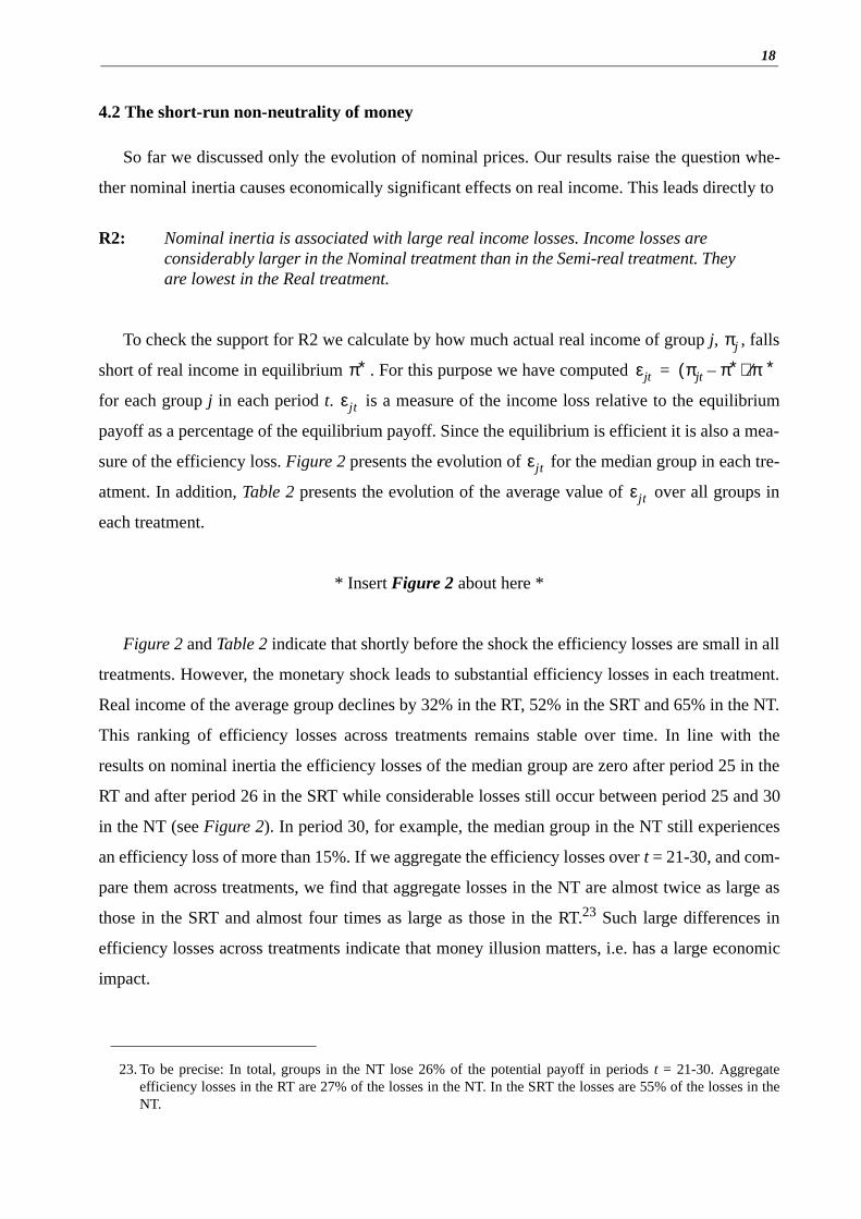
R2: Nominal inertia is associated with large real income losses. Income losses are considerably larger in the Nominal treatment than in the Semi-real treatment. They are lowest in the Real treatment.

To check the support for R2 we calculate by how much actual real income of group j, , falls

short of real income in equilibrium . For this purpose we have computed

for each group j in each period t. is a measure of the income loss relative to the equilibrium

payoff as a percentage of the equilibrium payoff. Since the equilibrium is efficient it is also a mea-

sure of the efficiency loss. Figure 2 presents the evolution of for the median group in each tre-

atment. In addition, Table 2 presents the evolution of the average value of over all groups in

each treatment.

* Insert Figure 2 about here *

Figure 2 and Table 2 indicate that shortly before the shock the efficiency losses are small in all

treatments. However, the monetary shock leads to substantial efficiency losses in each treatment.

Real income of the average group declines by 32% in the RT, 52% in the SRT and 65% in the NT.

This ranking of efficiency losses across treatments remains stable over time. In line with the

results on nominal inertia the efficiency losses of the median group are zero after period 25 in the

RT and after period 26 in the SRT while considerable losses still occur between period 25 and 30

in the NT (see Figure 2). In period 30, for example, the median group in the NT still experiences

an efficiency loss of more than 15%. If we aggregate the efficiency losses over t = 21-30, and com-

pare them across treatments, we find that aggregate losses in the NT are almost twice as large as

those in the SRT and almost four times as large as those in the RT.23 Such large differences in

efficiency losses across treatments indicate that money illusion matters, i.e. has a large economic

impact.

23. To be precise: In total, groups in the NT lose 26% of the potential payoff in periods t = 21-30. Aggregateefficiency losses in the RT are 27% of the losses in the NT. In the SRT the losses are 55% of the losses in theNT.

πj

π∗ εjt πjt π∗–( ) π∗⁄=

εjt

εjt

εjt

19

4.3 Long-run adjustment to equilibrium?

One of the core propositions of modern macroeconomics is that in the long run money is neu-

tral. In the absence of multiple equilibria and hysteresis effects, as described, for example in Blan-

chard and Summers (1986), there are good theoretical reasons for long-run neutrality. Yet, we are

not aware of direct and unambiguous evidence in favour of long-run neutrality.24 In the context of

our simple laboratory economy we get, however, clear evidence that in the long run nominal prices

adjust rather close to the new equilibrium.The result is summarized in

R3: In the long run, i.e., towards the end of the post-shock phase actual nominal prices adjust close to the equilibrium in all three treatment conditions and the real effects of money vanish.

R3 also means that in the long run money illusion has no impact on behavior because equili-

brium is reached in each treatment. Support for R3 comes from Figure 1, and Tables 2 and 3.

Figure 1 shows that the median group is exactly in equilibrium in each treatment in periods 36-40.

Table 3 indicates that during these periods 69% of all group observations are exactly in equili-

brium in the NT while in the other two conditions even 76% of all group observations are exactly

in equilibrium. In addition, Table 2 shows that the deviations from equilibrium are small because

average prices are close to equilibrium in periods 36-40. Table 2 also shows that the real effects of

the money shock vanish over time because efficiency levels towards the end of the post-shock

phase are rather similar to the efficiency levels shortly before the shock. This indicates that money

is neutral in the long run.

24. In the survey paper on the real effects of money in the Handbook of Monetary Economics Blanchard (1990:828) writes for example: The long-run neutrality of money “is very much a matter of faith, based on theoreticalconsiderations rather than on empirical evidence“. In the meantime, however, several empirical studies areavailable. Fisher and Seater (1993) reject the long-run neutrality of money for the U.S. Yet, Boschen and Otrok(1994) question these results.They argue that if one accounts for the exceptional period from 1930 to 1939(when an extraordinary number of bank failures occurred) by a dummy variable, long-run neutrality prevailsfor U.S. data. Haug and Lucas (1997) provide independent evidence that the rejection of long-run neutrality byFisher and Seater is based on the anomalous period of the 1930’s. Lucas (1996) provides data suggesting thatlong-run neutrality is the rule rather than the exception. In contrast, Ball’s (1998) empirical study indicates thatmoney shocks have long-run effects by changing the equilibrium unemployment rate.

20

4.4 Causes of nominal inertia

In principle, there are at least two potential reasons for the substantial amount of nominal iner-

tia observed in our experiment. First, it may be the case that subjects are simply confused after the

monetary shock and do no longer play best replies to their expectations. The near-rationality

approach, for example, assumes that a fraction of subjects fails to maximize after a monetary

shock because the losses associated with non-adjustment are small. In our experiment some sub-

jects may also be somehow anchored at the “historically“ given pre-shock price level so that they

do not play best reply. Second, it may be that nominal inertia is caused by sticky expectations.

Subjects may believe that the prices of other agents remain relatively high and play best reply to

this expectation. Due to strategic complementarity their own price will then also be relatively

high.

With regard to best reply behavior the following result emerges from our analysis:

R4: In all treatment conditions and all periods a large majority of subjects playsexactly a best reply to . On average, deviations from the best reply are smallin each treatment.

* Insert Figure 3 about here *

Support for R4 is provided by Figure 3. In this figure we show the evolution of the percentage

of subjects who play exactly best reply to their expectation . Before the shock this percentage

is between 70 and 90 percent. Immediately after the shock there is a relatively small drop in the

percentage of best replies. However, those subjects who deviate are, in general, playing relatively

close to the best reply. Additional information on best reply behavior is provided by Figure 4. This

figure compares, for given intervals of price expectations , the average best reply with the

average level of the actually chosen nominal prices in periods 21-25.25 The numbers above the

bars indicate the relative frequency of price observations in the respective intervals. In the NT, for

example, 14 percent of all price expectations fall within the interval 16-18 (see top diagram of

the figure). Figure 4 indicates that for any interval the deviation of actual average prices from the

average best reply is relatively small in the NT. The same holds true for the SRT and the RT .26

25. The best reply for x- and y-type subjects is weakly monotonic in . The impression of the non-monotonicityof best replies in Figure 4 is created by the fact that we aggregated over x and y types and that the relative fre-quency of x- and y-types differs across expectation intervals. Based on tests for differences in best reply beha-vior across types we conclude that aggregation over types is unproblematic.

P i–e

P i–e

P i–e

P i–

P i–e

21

* Insert Figure 4 about here *

Next we summarize our main result with regard to price expectations :

R5: In all treatment conditions there is some inertia in price expectations after the shock. However, price expectations exhibit much more inertia in the Nominal treat-ment compared to the other two treatment conditions.

Support for R5 is provided by Figure 5 and Table 4. Figure 5 describes the evolution of the

average expectation of the median group over time.27 This picture is qualitatively strikingly simi-

lar to Figure 1 which shows the evolution of average prices of the median group. In all three treat-

ments price expectations exhibit some inertia but in the NT expectations are much more sticky.

The jump in price expectations immediately after the shock is more than twice as big in the RT and

the SRT as in the NT. Moreover, while it takes 5 and 7 periods, respectively, until expectations

reach the equilibrium in the RT and the SRT, it takes 14 periods until equilibrium expectations pre-

vail in the NT.

* Insert Figure 5 about here *

* Insert Table 4 about here *

Table 4 reveals that the evolution of average expectations (over all groups) follows roughly the

same pattern as the evolution of average expectations of the median group. Expectations exhibit

some stickiness in all three treatments immediately after the shock but the stickiness is much lar-

ger and adjustment takes much longer in the NT. Information about the inertia of expectations is

also provided by Figure 4. The top diagram in Figure 4 indicates, for example, that, in periods 21-

25, 66% of price expectations in the NT are strictly above . In contrast, only 22% of

price expectation in the RT or the SRT are above 9. This can be considered as rather strong evi-

dence that expectations do not jump to the new post shock equilibrium values and that the speed

with which expectations adjust, is much lower in the NT.

26. In the Semi-real and the Real treatment we occasionally observe relatively “large“ deviations from best replybehavior (e.g. in the interval 19-21 in the bottom diagram). However, these deviations are, in general, outlyerswhich is indicated by the small number of observations in the corresponding intervals.

27. The unit of observation is the average over all -values in a group.

P i–e

Pe

i–

Pe

i– 9=

22

5. Interpretation and concluding remarks

At a superficial level it seems that money illusion does not fit well into the maximizing frame-

work of modern economics. However, simple game-theoretic reasoning shows that in interactive

situations with strategic complementarity the conditions for the absence of behavioral effects of

money illusion are extremely demanding. Paraphrasing Abraham Lincoln28, one can say that, to

render money illusion behaviorally relevant, it is neither necessary to fool all the people some of

the time nor some of the people all the time, not to speak of fooling all the people all the time. It is

not even necessary that there are “fools“, i. e., people with money illusion. All that is needed is

that there are some people who believe that others believe, etc., that money illusion leads to less

than full adjustment of nominal prices after a nominal shock. As long as such beliefs prevail ratio-

nal individuals find it in their interest to not fully adjust their nominal prices, either.

The results of our experiments unambiguously show that people do not expect full price adju-

stment after a nominal shock. Moreover, as Figure 5 shows, our results leave little doubt that in the

Nominal Treatment the stickiness of price expectations is much larger than in the Real or the

Semi-real Treatment. The veil of money that is incorporated in the Nominal Treatment is thus

responsible for much of the inertia in price expectations. In the presence of strategic complementa-

rity and best reply behavior this inertia in price expectations causes, in turn, inertia in price

choices. Therefore, in period t+1 subjects have little reason to make big adjustments in price

expectations after they observed the rather small adjustment of aggregate prices in period t. The

small adjustment in expectations in t+1 again provides an incentive to change prices in period t+1

only a little. Thus, small adjustments in expectations cause small adjustments in actual prices

which in turn render only small adjustments in expectations reasonable. The overall result of these

incremental changes in expectations and prices is a rather slow convergence to the equilibrium

which is associated with substantial income losses during the adjustment phase.

Most business transactions are shrouded in nominal money and the smallest nominal accoun-

ting unit is kept constant despite frequent changes in the money supply and nominal prices. Our

Nominal Treatment captures these two important features of economic life. In other dimensions,

however, our experimental design is simpler by orders of magnitude. The representation of the

28. In his speech on 8 Sept. 1858 A. Lincoln said: “You can fool all the people some of the time, and some of thepeople all the time, but you cannot fool all the people all the time.“

23

strategic situation by payoff matrices makes it rather easy to find the best reply for a given price

expectation. In contrast, in naturally occurring environments the nature of the decision problems

and of strategic interaction may render it quite difficult to find best replies. As a consequence,

nominal inertia due to near rationality is more likely to prevail. In the Nominal Treatment we trai-

ned subjects how to compute real payoffs from the nominal payoff table and the experiment did

not start before everybody had correctly solved the training exercises. In naturally occurring envi-

ronments no similar educational measures precede nominal shocks. It is, thus, more likely that

beliefs about the prevalence of money illusion exist. In addition, in our experiment subjects recei-

ved unambiguous feedback information about the aggregate price level at the end of each period.

In reality, the relevant information signals are probably much more noisy and there is much more

information to consider. Therefore, the formation of rational expectations is more complicated.

Taken together, this suggests that we created an experimental environment which is relatively

hostile to money illusion and nominal inertia. Yet, since money illusion has behavioral effects

even in such a simple environment there is little reason to believe that it is irrelevant in more com-

plicated environments.

In view of the simplicity of our experimental environment and because of the training proce-

dure before the start of the experiment it seems unlikely that subjects themselves suffered from

money illusion. In our view it is more likely that money illusion prevailed at a higher belief level,

that is, that subjects expected others to suffer, or expected that others expected others to suffer, etc.

from money illusion. The fact that subjects expect relatively small price adjustments after the

shock in the Nominal Treatment also suggests that this interpretation is correct. In a more compli-

cated environment, however, it seems more likely that at least some people suffer from money

illusion themselves.

24

References

Akerlof, G.A. and Yellen, J.L. (1985): A Near Rational Model of the Business Cycle, with Wageand Price Inertia. Quarterly Journal of Economics, 100: 823-38.

Akerlof, G.A.; Dickens, W.T. and Perry, G.L. (1996): The Macroeconomics of Low Inflation.Brookings Papers on Economic Activity, (1): 1-76.

Ball, L. (1998): Disinflation and the NAIRU, in: C.D. Romer and D.H. Romer (eds.): ReducingInflation. Motivation and Strategy. University of Chicago Press.

Ball, L. and Romer, D. (1987): Sticky Prices as a Coordination Failure. New York University.Mimeo.

Belongia, M.T. (1996): Measurement Matters: Recent Results from Monetary EconomicsReexamined. Journal of Political Economy, 104(5): 1065-83.

Bernanke, B.S. and Carey, K. (1996): Nominal Wage Stickiness and Aggregate Supply in theGreat Depression. Quarterly Journal of Economics, 111: 853-84.

Blanchard, O.J. (1990): Why does Money affect Output? A Suvey. In: B.M. Friedman and F.M.Hahn (eds.): Handbook of Monetary Economics, Vol. 2, North-Holland: Amsterdam: 779-835.

Blanchard, O.J. and Kiyotaki, N. (1987): Monopolistic Competition and the Effects of AggregateDemand. American Economic Review, 77(4): 647-66.

Blanchard, O.J. and Summers, L.H. (1986): Hysteresis and the European Unemployment Problem.NBER Macroeconomics Annual, 1: 15-78.

Boschen, J.F. and Otrok, C.M. (1994): Long-Run Non-Neutrality and Superneutrality in anARIMA Framework: Comment. American Economic Review, 84(5): 1470-3.

Bryant, J. (1983): A Simple Rational Expectations Keynes-Type Model. Quarterly Journal ofEconomics, 98(Aug.): 525-8.

Coleman, W.J. (1996): Money and Output: A Test of Reverse Causation. American EconomicReview, 86(1): 90-111.

Cooper, R.W. and Haltiwanger, J. (1993): Evidence on Macroeconomic Complementarities.NBER Working Paper no. 4577.

Diamond, P.A. (1982): Aggregate Demand Management in Search Equilibrium. Journal of Politi-cal Economy, 90(Oct.): 881-94.

Fischer, S. (1977): Long-Term Contracts, Rational Expectations, and the Optimal Money SupplyRule. Journal of Political Economy, 85 (1): 191-205.

Fisher, I. (1928): The Money Illusion. Longmans: Toronto.

Fisher, M.E. and Seater, J.J. (1993): Long-Run Neutrality and Superneutrality in an ARIMA Fra-mework. American Economic Review, 83(3): 402-15

Friedman, B.M. and Hahn, F.M. (1990): Handbook of Monetary Economics. Vol. 2, North-Hol-land: Amsterdam.

Haltiwanger, J. and Waldman, M. (1985): Rational Expectations and the Limits of Rationality: AnAnalysis of Heterogeneity. American Economic Review, 75(3): 326-40.

25

Haltiwanger, J. and Waldman, M. (1989): Rational Expectations and Strategic Complements: TheImplications for Macroeconomics. Quarterly Journal of Economics, 104 (August): 463-84.

Haug, A.A. and Lucas, R.E. Jr. (1997): Long-Run Neutrality and Superneutrality in an ARIMAFramework: Comment. American Economic Review, 87(4): 756-759.

Ho, T.H. Weigelt, K. and Camerer, C. (1996): Iterated Dominance and Learning in Experimental‘Beauty Contest’Games. forthcoming: American Economic Review.

Hoover, K.D. and Perez, S.J. (1994): Post hoc ergo propter hoc once more: An evaluation of ‘DoesMoney Matter?’ in the spirit of James Tobin. Journal of Monetary Economics, 34: 75-88.

Howitt, P. (1989): Money Illusion. In: J Eatwell, M. Milgate and P. Newman (eds.): Money. W. W.Norton: New York, London: 244-247.

Kahn, S. (1995): Evidence of Nominal Wage Stickiness. Working Paper, Boston University Schoolof Management (Aug. 1995).

Leontief, W. (1936): The Fundamental Assumptions of Mr. Keynes’ Monetary Theory of Unem-ployment. Quarterly Journal of Economics, 5(Nov.): 192-197.

Lucas, R.E. Jr. (1972): Expectations and the Neutrality of Money. Journal of Economic Theory,4(April): 103-24.

Lucas, R.E. Jr. (1996): Nobel Lecture: Monetary Neutrality. Journal of Political Economy, 104(4):661-82.

Mankiw, N.G. (1985): Small Menu Costs and Large Business Cycles: A Macroeconomic Model ofMonopoly. Quarterly Journal of Economics, 100(May): 529-537.

Mankiw, N.G. and Romer, D.H. (eds.) (1991): New Keynesian Economics. Vol. 1 & Vol. 2, MITPress: Cambridge, MA.

Nagel, R. (1995): Unraveling in Guessing Games: An Experimental Study. American EconomicReview, 85(5): 1313-26.

Oh, S. and Waldman, M. (1994): Strategic Complementarity Slows Macroeconomic Adjustmentto Temporary Shocks. Economic Inquiry, 32(April): 318-29.

Patinkin, D. (1949): The Indeterminacy of Absolute Prices in Classical Economic Theory. Econo-metrica 17(1): 1-27.

Romer, C.D. and Romer, D.H. (1989): Does monetary policy matter? A new test in the Spirit ofFriedman and Schwartz. NBER Macroeconomics Annual 4 : 121.

Romer, C.D. and Romer, D.H. (1994): Monetary Policy Matters. Journal of Monetary Economics,34: 75-88.

Russell, T. and Thaler, R.H. (1985) The Relevance of Quasi-Rationality in Competitive Markets.American Economic Review, 75(5): 1071-82.

Selten, R. and Berg, C.C. (1970): Drei experimentelle Oligopolserien mit kontinuierlichem Zeit-ablauf, in: H. Sauermann (ed.): Beiträge zur experimentellen Wirtschaftsforschung, Vol. II,Tübingen: 162-221.

Shafir, E.; Diamond, P.A. and Tversky, A. (1997): On Money Illusion. Quarterly Journal of Eco-nomics, 112(May): 341-74.

Smith, V.L., Suchanek, G.L. and Williams, A.W. (1988): Bubbles, Crashes, and EndogenousExpectations in Experimental Spot Asset Markets. Econometrica, 56(6): 1119-52.

26

Taylor, J.B. (1979): Staggered Wage Setting in a Macro Model. American Economic Review,69(2): 108-113.

Taylor, J.B. (1997): A Core of Practical Macroeconomics. American Economic Review, Papersand Proceedings 87(2): 233-5.

Tobin, J. (1972): Inflation and Unemployment. American Economic Review, 62: 1-18.

Tversky, A. and Kahneman, D. (1981): The Framing of Decisions and the Psychology of Choice.Science 211: 453-8.

Tversky, A. and Kahneman, D. (1986): Rational Choice and the Framing of Decisions. Journal ofBusiness 49(4): 251-78.

27

Appendix A – Functional specification of payoffs

As explained in detail in section 3.1 our specification of subjects’ payoff functions served

several purposes. A particularly important purpose was to rule out that the adjustment to the equi-

librium is confounded by subjects’ attempts to achieve out-of-equilibrium cooperative gains. Note

that this purpose rules out payoff functions that are derived from oligopolistic or monopolistic

competition among firms. We achieved our aim by the payoff functions below because they imply

that the equilibrium is the only efficient point in payoff space.

Note also that the equilibrium price for each individual i is a best reply not only to the equili-

brium expectation for but also to out-of-equilibrium expectations that are close to the equili-

brium expectation (see also payoff tables T1-T6 in Appendix C below). This feature of the payoff

functions speeds up adjustment to equilibrium behavior because it ensures that the equilibrium

price choice is also a best reply for expectations that are not exactly in equilibrium. The arctan-

function in the denominator reflects this property of the payoff functions.

The real payoff for agent i of type k = x, y is given by:

In all periods and all experimental sessions the parameters a, b, c, d, e, f and V were the same.

They were given by a = 0.5, b = 0.6, c = 27, d = 1, e = 0.05 , f = 20 and V = 40.

is the actual average price of the other n-1 players from the viewpoint of player i who is

of type k. is the equilibrium average price of the other n- 1 players from the viewpoint of a

player of type k. is the actual price of i who is of type k. is the equilibrium price of a

player of type k.

P i–

πik

V

1 aP ik–

M---------

P k

M--------–

+

1 bP ik–

M---------

P∗k

M--------–

2

+

---------------------------------------------⋅

1 cPik

M-------

P∗kM

--------– d

P ik–

M---------

P∗k

M--------–

– e arcP ik–

M---------

P∗k

M--------–

f⋅tan⋅+

2

+

------------------------------------------------------------------------------------------------------------------------------------------------------------------=

P ik–

P∗k

Pik P∗k

28

Appendix B – InstructionsThe original instructions were in German. This section reprints a translation of the instructions

used in the Nominal treatment for agents of type y.

General instructions for participants

You are participating in a scientific experiment which is funded by the Swiss National ScienceFoundation. The purpose of this experiment is to analyze decision making in experimental mar-kets. If you read instructions carefully and take appropriate decisions, you may earn a considerableamount of money. At the end of the experiment all the money you earned will be immediately paidout in cash.

Each participant is paid SFr.15.- for showing up. During the experiment your income will notbe calculated in Swiss Francs but in points. The total amount of points you collected during theexperiment will be converted into Swiss Francs, by applying the following exchange rate:

10 Points = 15 centimes.

Here is a brief description of the experiment. A more detailed description is given below. Allparticipants are in the role of firms, selling some product. In this experiment, there are two typesof firms: firms of type x and firms of type y. Each firm has to choose a selling price in everyperiod. The income you earn depends on the price you choose and on the prices all other firmschoose.

During the experiment you are not allowed to communicate with any other participant. Ifyou have any questions, the experimenters will be glad to answer them. If you do not followthese instructions you will be excluded from the experiment and deprived of all payments.

The following pages describe the procedures of the experiment in detail.

Detailed information for firms of type y

This experiment lasts 20 periods plus one trial period. You are not paid for the trial period. Youshould nevertheless take the trial period seriously since you may gain experience in this period.This experience helps you to take decisions in the other periods which are paid out. You are in therole of a firm, just as all other participants in this experiment. All participants are in groups of 4,i.e. every participant is in a group with three other firms. There are two firms of type x and twofirms of type y in every group.

You are a firm of type y

Consequently, there are two other firms of type x and one more firm of type y in your group.No participant knows which persons are in his or her group. Yet, everybody knows that the groupcomposition remains constant throughout the experiment. The decisions taken by other groups areirrelevant for your group.

In every period all firms simultaneously decide which selling price they set for the currentperiod. Every firm has to choose an integer price from the interval

.1 selling price 30≤ ≤

29

How much you earn depends on the price you choose and on the average price of all otherfirms in your group. Independent of the type, the average price for every firm is calculated by thefollowing formula:

Average price = (Sum of selling prices of other 3 firms) / 3

Consequently, the average price will be in the interval

.

The average price is rounded to the next integer number.

How to read the income table for a firm of type y

The green income table shows your nominal income in points if you choose a specific priceand a specific average price results in this period (see separate table). Your income at the end ofthe experiment is not based on nominal point income, but on real point income. The followingrelation between the two holds:

Real income = Nominal income / Average price of other firms

This formula holds for all firms. The real point income that will be paid out is rounded in everyperiod to the next integer number.

Example:Suppose, you choose a price of 2 and the actual average price is 4. In this case your nominal point income is 29points. Your (rounded) real income is 7 points (= 23 / 4).

When you decide which price to choose, you do not yet know which average price willactually result in this period. The green income table can consequently help you to calculate yourreal point income given your expectation on the average price of other firms.

Example:Given an expectation on the average price you can read off the green table the payoff you get when choosing dif-ferent selling prices. For example, if you expect an average price of 30 and choose a price of 17, your expectednominal income is 141 points, your expected real income is 5 points (= 141 / 30). If you choose a price of 10 atthis expected price, your expected nominal income is 86 points, your expected real income 3 points (= 86 / 30).

Please note that you are in a group with one firm of type y and two firms of type x. To deter-mine the income of the other firm of type y, you have to use the green table. To determine theincome of the other two firms of type x, you have to use the blue income table. This table alsoshows nominal income in points. The same formula above is used to calculate real payoffs forfirms of type x.

What the screens show

On both screens described below the current period is indicated in the upper left corner, and theupper right corner displays remaining time in seconds to decide or to view the screen.

The upper half of the input screen (see figure on next page) has three cells, where you canenter data into the computer.

1 average price 30≤ ≤

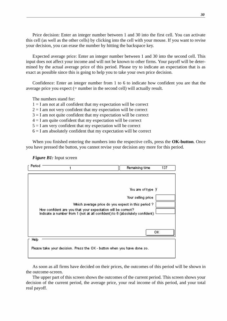
30

Price decision: Enter an integer number between 1 and 30 into the first cell. You can activatethis cell (as well as the other cells) by clicking into the cell with your mouse. If you want to reviseyour decision, you can erase the number by hitting the backspace key.

Expected average price: Enter an integer number between 1 and 30 into the second cell. Thisinput does not affect your income and will not be known to other firms. Your payoff will be deter-mined by the actual average price of this period. Please try to indicate an expectation that is asexact as possible since this is going to help you to take your own price decision.

Confidence: Enter an integer number from 1 to 6 to indicate how confident you are that theaverage price you expect (= number in the second cell) will actually result.

The numbers stand for:1 = I am not at all confident that my expectation will be correct2 = I am not very confident that my expectation will be correct3 = I am not quite confident that my expectation will be correct4 = I am quite confident that my expectation will be correct5 = I am very confident that my expectation will be correct6 = I am absolutely confident that my expectation will be correct

When you finished entering the numbers into the respective cells, press the OK-button. Onceyou have pressed the button, you cannot revise your decision any more for this period.

Figure B1: Input screen

As soon as all firms have decided on their prices, the outcomes of this period will be shown inthe outcome-screen.

The upper part of this screen shows the outcomes of the current period. This screen shows yourdecision of the current period, the average price, your real income of this period, and your totalreal payoff.

\

31

The lower part of this screen displays the outcomes of past periods.

Figure B2: Outcome screen

Overview: What you have to do in every period.

In every period every firm has to choose a price. Every integer price from 1 to 30 can be chosen .

• Enter your price decision into the first cell of the input screen. • Enter into the second cell the average you expect for this period

. • Enter your confidence in your price expectation into the third cell (numbers 1 to 6).

When you have completed the three cells, press the OK-Button. The remaining time to takeyour decisions is shown in the upper right corner of the screen.

When all participants have taken their decisions, or when the time has elapsed, all participantsare shown the outcome screen. This screen shows your decisions, actual average prices and yourreal payoff in points for the current and the past periods.

To take your decisions the following aids are at your disposal:Greenincome table: Helps you to estimate your expected nominal point income (You are a firm of

type y). Your payoff is determined by your real income in points. You can calculate your real income from the nominal income (= numbersshown in the income table) by applying the following formula:

1 selling price 30≤ ≤

1 expected average price 30≤ ≤

32

Real income = Nominal income / Average price of other firmsBlueincome table: Helps to estimate the nominal point income of the firms of type x in your

group. The payoff of these firms are also determined by their real pointincome. To calculate the real income of firms of type x, you also apply theformula above.

Outcome screen: Displays your selling price, the actual average price and your real income forthe present and the past periods.

Do you have any questions?

Control questions

You have to answer all of the following questions. If you do not answer a question, you will beexcluded from the experiment and all payments. Wrong answers do not have any consequences. Ifyou have any questions, please ask us.

1. Please indicate an expectation for the average price of other firms from 1 to 30.Expected average price ............................

2. Please indicate a selling price from 1 to 30.Selling price ............................

3) What is your expected nominal income in points at the prices you indicated in 1) and 2)?Your nominal income ............................

4. What is your expected real income in points at the prices you indicated in 1) and 2)?Your real income ............................

5. Suppose you choose a price of 1. The other firm of type y chooses a price of 30. The first firmof type x chooses a price of 7 and the second firm of type x chooses a price of 23.

a) What is your average price at the (fictitious) prices? ............................What is your nominal income? ............................What is your real income? ............................

b) What is the average price of the other firm of type y?............................What is the nominal income of this firm? ............................What is the real income of this firm? ............................

c) What is the average price of the first firm of type x? ............................What is the nominal income of this firm? ............................What is the real income of this firm? ............................

d) What is the average price of the second firm of type x?............................What is the nominal income of this firm? ............................What is the real income of this firm? ............................

33

Table 1: Experimental design

Nominal treatment Semi-real treatment Real treatment

All

peri

ods

Representation of payoffs nominal real real

Smallest nominal account-ing unit

constant(variation in real terms)

constant(variation in real terms)

adjusted to keep real accounting unit constant

Group size n = 4 n = 4 n = 4

Information feedback in period t

Real equilibrium payoff(pre- and post-shock, for both types)

40 40 40

Pre

-sho

ck (

t = 1

- 2

0)

Choice variable

Money supply 42 42 42

Average equilibrium price

and average equilib-rium expectation for the whole group

18 18 18

Equilibrium price for type x 9 9 9

Equilibrium expectation

for type x21 21 21

Equilibrium price for type y 27 27 27

Equilibrium expectation

for type y15 15 15

Pos

t-sh

ock

(t =

21

- 40

)

Choice variable

Money supply 14 14 14

Average equilibrium price

and average equilib-rium expectation for the whole group

6 6 6

Equilibrium price for type x 3 3 3

Equilibrium expectation

for type x7 7 7

Equilibrium price for type y 9 9 9

Equilibrium expectation

for type y5 5 5

P i– πi( ) πi( ) πi( )

P i– πi, P i– πi, P i– πi,

Pi 1 2, … 30,{ , }∈ Pi 1 2, … 30,{ , }∈ Pi 3 6, … 90,{ , }∈

M0

P∗

P i–e

Pie

Pi 1 2, … 30,{ , }∈ Pi 1 2, … 30,{ , }∈ Pi 1 2, … 30,{ , }∈

M1

P∗

P i–e

P i–e

34

Table 2: Evolution of prices and efficiency losses over time (all entries rounded to integers)

Average price of the median group

Average price Average efficiency loss (percent)

periodNominal treatment

Semi-realtreatment

Real treatment

Nominal treatment

Semi-realtreatment

Real treatment

Nominal treatment

Semi-realtreatment

Real treatment

18 18 18 18 19 18 19 3 4 3

19 18 18 18 18 18 21 1 2 12

20 18 18 18 18 18 21 1 1 9

21 13 9 8 13 9 8 65 52 32

22 13 7 7 13 8 7 47 20 11

23 11 7 6 11 7 7 35 15 5

24 10 7 6 10 7 7 27 9 6

25 9 6 6 10 7 7 17 15 5

26 10 6 6 10 7 6 16 8 4

27 10 6 6 10 6 6 16 4 1

28 9 6 6 9 6 6 11 5 1

29 8 6 6 9 6 6 9 4 1

30 7 6 6 9 7 6 14 11 2

31 6 6 6 8 6 7 8 5 10

32 6 6 6 8 6 6 6 3 6

33 6 6 6 7 6 6 6 2 3

34 6 6 6 7 6 6 5 3 0

35 6 6 6 7 6 6 3 3 0

36 6 6 6 7 6 7 10 2 10

37 6 6 6 7 6 7 5 1 3

38 6 6 6 7 6 7 14 2 4

39 6 6 6 7 6 7 12 1 12

40 6 6 6 7 6 7 2 3 7

35

Table 3: Percentage of price observations above, in and below the equilibrium (group averages as units of observation)

Nominal (n =11) Semi-Real (n =10) Real (n =10)

Period above in below above in below above in below

21 - 25 93 7 0 82 16 2 52 34 14

26 - 30 58 42 0 28 70 2 14 82 4

31 - 35 42 56 2 22 74 4 22 78 0

36 - 40 31 69 0 22 76 2 24 76 0

36

Table 4: Evolution of expectations

Average expectation of the median group Average expectation

periodNominal treatment

Semi-real treatment

Real treatment

Nominal treatment

Semi-real treatment

Real treatment

18 18 18 18 19 18 20

19 18 18 18 19 18 20

20 18 18 18 18 18 22

21 14 9 9 14 10 9

22 13 9 8 13 8 8

23 12 8 6 13 8 7

24 12 7 7 12 8 7

25 11 7 6 11 7 7

26 11 7 6 10 7 6

27 10 6 6 10 7 6

28 9 6 6 10 7 6

29 8 6 6 9 7 6

30 8 6 6 9 6 6

31 7 6 6 9 6 6

32 7 6 6 8 6 6

33 7 6 6 8 6 6

34 6 6 6 7 6 6

35 6 6 6 7 6 6

36 6 6 6 7 6 6

37 6 6 6 7 6 7

38 6 6 6 7 6 7

39 6 6 6 7 6 7

40 6 6 6 7 6 7

37

Figure 1: Nominal average prices of median group by treatment

0

2

4

6

8

10

12

14

16

18

20

18 19 20 21 22 23 24 25 26 27 28 29 30 31 32 33 34 35 36 37 38 39 40

Nominal

Semi-Real

Real

38

Figure 2: Efficiency losses of the median group

-0.7

-0.6

-0.5

-0.4

-0.3

-0.2

-0.1

0

18 19 20 21 22 23 24 25 26 27 28 29 30 31 32 33 34 35 36 37 38 39 40

Nominal

Semi-real

Real

Period

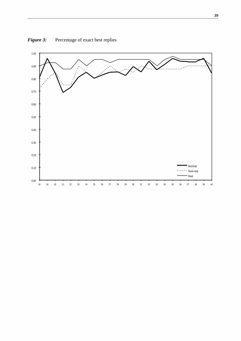
39

Figure 3: Percentage of exact best replies

0.00

0.10

0.20

0.30

0.40

0.50

0.60

0.70

0.80

0.90

1.00

18 19 20 21 22 23 24 25 26 27 28 29 30 31 32 33 34 35 36 37 38 39 40

Nominal

Semi-real

Real

40

Figure 4: Actual average prices and average best reply for given expectations by treatment

(cumulative for periods 21 - 25)

Semi-real treatment

Real treatment

Semi-real treatment

Nominal treatment

0

5

10

15

20

25

30

1-3 4-6 7-9 10-12 13-15 16-18 19-21 22-24 25-27 28-30

average best reply

actual average price

0.01

Expected price

0.27

0.020.02

0.170.51

0.01

0

5

10

15

20

25

30

1-3 4-6 7-9 10-12 13-15 16-18 19-21 22-24 25-27 28-30

average best reply

actual average price

0.100.24

0 20

0.14

0.02

0.01

Expected price

0.07

0.02

0 20

0

5

10

15

20

25

30

1-3 4-6 7-9 10-12 13-15 16-18 19-21 22-24 25-27 28-30

average best reply

actual average price

0.33

Expected price

0.01

0.02

0.18

0.45

0.01

41

Figure 5: Expectation of the median group by treatment

0

2

4

6

8

10

12

14

16

18

20

18 19 20 21 22 23 24 25 26 27 28 29 30 31 32 33 34 35 36 37 38 39 40

Nominal

Semi-real

Real

Period

42

Payoff Table T1: Nominal, pre-shock, Type yAverage price of other firms

1 2 3 4 5 6 7 8 9 10 11 12 13 14 15 16 17 18 19 20 21 22 23 24 25 26 27 28 29 30elling price

1 9 16 22 27 31 34 37 39 41 42 44 45 47 50 53 56 58 59 60 59 59 58 58 57 56 55 54 53 52 51

2 10 18 24 29 34 37 40 42 44 46 47 49 51 53 57 60 63 63 64 63 63 62 61 60 59 58 57 56 55 54

3 11 20 27 33 37 41 44 46 48 50 51 53 55 57 61 65 67 68 68 68 67 66 65 64 63 62 60 59 58 57

4 12 22 30 36 41 44 48 50 52 54 55 57 59 62 66 70 72 73 73 73 72 71 69 68 67 65 64 63 61 60

5 14 24 33 40 45 49 53 55 57 59 60 62 64 67 71 76 78 79 79 78 77 76 74 73 71 70 68 66 65 63

6 16 28 37 45 50 55 58 61 63 64 66 67 69 73 77 82 85 86 85 84 83 81 79 78 76 74 72 70 69 67

7 18 31 42 50 56 61 64 67 69 70 72 73 76 79 84 89 92 93 92 91 89 87 85 83 81 79 77 75 73 71

8 20 36 47 56 63 68 72 74 76 78 79 80 83 86 92 97 101 101 100 99 97 94 92 89 87 84 82 80 78 76

9 23 40 54 64 71 76 80 83 84 86 87 88 91 95 101 107 110 110 109 107 105 102 99 96 93 90 88 85 83 80

10 26 46 61 72 80 86 90 92 94 95 96 97 100 104 111 117 121 121 119 117 114 110 107 104 100 97 94 91 88 86

11 29 51 69 81 90 97 101 103 105 106 107 108 110 115 122 129 133 133 131 128 124 120 116 112 108 104 101 97 94 91

12 32 58 77 92 102 109 114 116 118 118 119 120 122 127 135 143 147 147 144 140 136 131 126 121 117 113 109 105 101 98

13 35 64 87 104 116 123 128 131 132 133 133 134 136 141 150 159 163 162 159 154 149 143 138 132 127 122 117 113 109 104

14 37 70 96 116 130 140 145 148 149 149 149 149 152 157 167 177 181 180 176 170 164 157 150 144 138 132 127 122 117 112

15 39 74 105 129 146 157 164 168 169 168 168 168 170 176 187 198 203 201 196 189 181 173 165 158 151 144 138 132 126 121

16 40 78 113 141 162 176 185 189 191 191 190 189 191 198 210 223 227 225 218 209 201 191 182 173 165 157 150 143 136 130

17 39 79 117 151 177 195 207 213 216 216 214 214 216 223 237 251 256 253 245 235 223 212 201 191 181 172 163 155 148 141

18 37 78 119 157 189 213 229 239 243 244 243 242 244 252 268 283 289 285 275 263 250 236 223 211 199 189 179 170 161 153

19 35 74 117 159 197 227 250 264 272 274 274 274 276 285 303 321 327 322 311 296 280 264 249 234 221 208 196 186 176 167

20 32 69 112 156 199 236 266 287 300 306 308 309 312 323 343 363 370 364 351 334 315 296 278 261 245 230 216 204 192 182

21 29 63 104 149 195 239 277 306 326 337 343 346 351 364 387 409 418 412 397 378 356 334 312 292 273 256 240 225 211 199

22 25 57 95 139 186 234 279 317 346 365 377 385 393 408 434 459 470 465 449 427 403 377 352 328 306 285 266 249 233 219

23 23 50 85 126 173 223 273 319 357 387 407 421 434 453 482 511 524 521 506 483 456 426 397 369 343 319 297 276 258 241

24 20 45 76 113 158 206 259 311 358 398 429 452 471 495 527 559 578 579 566 544 515 483 450 417 387 358 332 308 287 267

25 18 40 67 101 142 188 240 295 349 398 439 472 500 530 565 601 625 633 627 608 579 545 509 472 437 403 373 345 320 297

26 16 35 60 89 126 169 219 273 330 386 436 480 517 552 591 629 660 679 682 671 646 613 574 534 494 456 420 387 358 331

27 14 31 53 79 112 151 196 248 305 364 421 473 519 560 600 640 678 709 727 727 712 683 645 603 559 516 475 437 402 370

28 12 28 47 70 99 134 175 223 277 335 395 452 505 550 591 631 676 720 753 771 770 751 719 677 631 583 537 493 453 416

29 11 24 41 62 87 118 155 198 248 304 363 422 478 526 565 605 654 708 758 795 814 811 790 754 708 658 607 558 512 469

30 10 22 37 55 77 104 137 175 221 272 328 386 442 490 527 565 616 677 741 796 836 855 851 827 788 739 686 631 579 530

43

Payoff Table T2: Nominal, post-shock, Type yAverage price of other firms

1 2 3 4 5 6 7 8 9 10 11 12 13 14 15 16 17 18 19 20 21 22 23 24 25 26 27 28 29 30selling price

1 9 14 16 17 20 23 22 21 20 19 18 17 16 15 14 13 13 12 12 11 11 10 10 9 9 9 8 8 8 8

2 12 18 21 22 26 29 28 26 24 22 21 19 18 17 16 15 14 13 13 12 12 11 11 10 10 9 9 9 8 8

3 18 25 28 29 34 37 35 32 29 27 25 23 21 19 18 17 16 15 14 13 13 12 11 11 10 10 10 9 9 9

4 26 36 39 40 45 49 45 40 36 33 29 27 24 22 21 19 18 17 16 15 14 13 13 11 11 11 10 10 10 9

5 35 52 56 56 62 67 60 53 46 40 36 32 29 26 24 22 20 19 18 16 15 15 14 13 12 12 11 11 10 10

6 40 71 81 81 89 95 83 70 60 51 44 39 34 31 28 25 23 21 20 18 17 16 15 14 14 12 12 12 11 11

7 35 80 109 115 129 137 119 97 80 66 56 48 42 37 33 30 27 24 22 21 19 18 17 16 15 14 13 13 12 11

8 25 68 119 151 176 193 172 139 111 89 73 61 52 45 39 35 31 28 26 24 22 20 19 17 16 15 14 13 13 12

9 18 50 102 157 200 236 237 201 158 123 98 79 66 56 48 42 37 33 30 27 25 23 21 19 18 17 16 15 14 13

10 12 34 74 129 176 226 279 275 229 177 136 107 86 71 59 51 44 39 35 31 28 26 23 22 20 19 17 16 15 14

11 9 24 51 92 129 173 253 318 312 255 195 148 115 92 75 63 54 46 41 36 32 29 27 24 22 21 19 18 17 16

12 7 18 36 63 89 121 189 284 357 348 281 212 160 124 98 80 67 57 49 43 38 34 30 28 25 23 21 20 19 17

13 5 13 26 45 62 84 131 210 316 395 382 305 229 172 132 104 84 70 59 51 45 39 35 32 29 26 24 22 21 19

14 4 10 19 33 45 60 91 145 232 347 433 416 331 246 183 140 110 89 74 62 53 46 41 36 33 30 27 25 23 21

15 3 8 15 25 34 44 66 102 161 254 379 470 449 355 262 194 148 116 93 77 65 56 48 43 38 34 31 28 26 24

16 3 6 12 19 26 34 49 73 112 176 277 410 506 481 378 278 206 156 122 98 81 68 58 50 44 39 35 32 29 26

17 2 5 10 15 20 26 37 54 81 123 192 300 440 541 513 402 294 217 164 127 102 84 70 60 52 46 41 36 33 30

18 2 4 8 12 16 21 29 42 60 89 134 207 322 471 576 544 425 310 227 171 133 107 87 73 62 54 47 41 37 34

19 2 4 7 10 14 17 24 33 46 66 97 145 223 344 500 611 575 448 326 238 179 139 111 91 76 64 56 49 43 39

20 1 3 6 9 11 14 19 27 37 51 72 105 156 238 365 530 645 606 470 341 249 186 144 115 94 79 67 58 50 44

21 1 2 5 7 10 12 16 22 30 40 56 78 112 166 253 386 559 679 636 492 357 259 194 150 119 97 81 69 59 52

22 1 2 4 6 8 10 14 18 24 32 44 60 84 120 177 267 407 588 712 666 514 372 270 202 156 124 101 84 71 61

23 1 2 4 5 7 8 12 15 20 27 35 48 65 90 128 187 282 428 616 745 695 536 387 280 209 161 128 104 87 73

24 1 2 3 5 6 8 10 13 17 22 29 38 51 69 95 135 197 296 449 645 778 725 558 402 291 217 167 132 108 89

25 1 2 3 4 6 7 9 11 15 19 24 32 41 55 73 101 143 207 311 469 673 811 754 580 417 301 224 172 136 111

26 1 2 3 4 5 6 8 10 13 16 21 26 34 44 58 78 107 150 218 325 490 701 843 783 601 432 312 232 178 141

27 1 1 2 3 4 5 7 9 11 14 18 22 28 36 47 61 82 112 157 227 339 510 728 875 813 623 447 322 239 183

28 1 1 2 3 4 5 6 8 10 12 15 19 24 30 39 50 65 86 117 164 237 353 530 755 908 842 644 461 332 247

29 1 1 2 3 4 4 6 7 9 11 13 17 21 26 32 41 52 68 90 123 171 247 367 550 784 940 870 666 477 343

30 0 1 2 3 3 4 5 6 8 10 12 15 18 22 27 34 43 55 72 95 128 179 257 381 570 811 972 899 687 491

44

Payoff Table T3: Semi-real, pre-shock, Type yAverage price of other firms

1 2 3 4 5 6 7 8 9 10 11 12 13 14 15 16 17 18 19 20 21 22 23 24 25 26 27 28 29 30selling price

1 9 8 7 7 6 6 5 5 5 4 4 4 4 4 4 4 3 3 3 3 3 3 3 2 2 2 2 2 2 2

2 10 9 8 7 7 6 6 5 5 5 4 4 4 4 4 4 4 4 3 3 3 3 3 3 2 2 2 2 2 2

3 11 10 9 8 7 7 6 6 5 5 5 4 4 4 4 4 4 4 4 3 3 3 3 3 3 2 2 2 2 2

4 12 11 10 9 8 7 7 6 6 5 5 5 5 4 4 4 4 4 4 4 3 3 3 3 3 3 2 2 2 2

5 14 12 11 10 9 8 8 7 6 6 5 5 5 5 5 5 5 4 4 4 4 3 3 3 3 3 3 2 2 2

6 16 14 12 11 10 9 8 8 7 6 6 6 5 5 5 5 5 5 4 4 4 4 3 3 3 3 3 3 2 2

7 18 16 14 13 11 10 9 8 8 7 7 6 6 6 6 6 5 5 5 5 4 4 4 3 3 3 3 3 3 2

8 20 18 16 14 13 11 10 9 8 8 7 7 6 6 6 6 6 6 5 5 5 4 4 4 3 3 3 3 3 3

9 23 20 18 16 14 13 11 10 9 9 8 7 7 7 7 7 6 6 6 5 5 5 4 4 4 3 3 3 3 3

10 26 23 20 18 16 14 13 12 10 10 9 8 8 7 7 7 7 7 6 6 5 5 5 4 4 4 3 3 3 3

11 29 26 23 20 18 16 14 13 12 11 10 9 8 8 8 8 8 7 7 6 6 5 5 5 4 4 4 3 3 3

12 32 29 26 23 20 18 16 15 13 12 11 10 9 9 9 9 9 8 8 7 6 6 5 5 5 4 4 4 3 3

13 35 32 29 26 23 21 18 16 15 13 12 11 10 10 10 10 10 9 8 8 7 7 6 6 5 5 4 4 4 3

14 37 35 32 29 26 23 21 19 17 15 14 12 12 11 11 11 11 10 9 9 8 7 7 6 6 5 5 4 4 4

15 39 37 35 32 29 26 23 21 19 17 15 14 13 13 12 12 12 11 10 9 9 8 7 7 6 6 5 5 4 4

16 40 39 38 35 32 29 26 24 21 19 17 16 15 14 14 14 13 13 11 10 10 9 8 7 7 6 6 5 5 4

17 39 40 39 38 35 33 30 27 24 22 19 18 17 16 16 16 15 14 13 12 11 10 9 8 7 7 6 6 5 5

18 37 39 40 39 38 36 33 30 27 24 22 20 19 18 18 18 17 16 14 13 12 11 10 9 8 7 7 6 6 5

19 35 37 39 40 39 38 36 33 30 27 25 23 21 20 20 20 19 18 16 15 13 12 11 10 9 8 7 7 6 6

20 32 35 37 39 40 39 38 36 33 31 28 26 24 23 23 23 22 20 18 17 15 13 12 11 10 9 8 7 7 6

21 29 32 35 37 39 40 40 38 36 34 31 29 27 26 26 26 25 23 21 19 17 15 14 12 11 10 9 8 7 7

22 25 29 32 35 37 39 40 40 38 37 34 32 30 29 29 29 28 26 24 21 19 17 15 14 12 11 10 9 8 7

23 23 25 28 32 35 37 39 40 40 39 37 35 33 32 32 32 31 29 27 24 22 19 17 15 14 12 11 10 9 8

24 20 23 25 28 32 34 37 39 40 40 39 38 36 35 35 35 34 32 30 27 25 22 20 17 15 14 12 11 10 9

25 18 20 22 25 28 31 34 37 39 40 40 39 38 38 38 38 37 35 33 30 28 25 22 20 17 16 14 12 11 10

26 16 18 20 22 25 28 31 34 37 39 40 40 40 39 39 39 39 38 36 34 31 28 25 22 20 18 16 14 12 11

27 14 16 18 20 22 25 28 31 34 36 38 39 40 40 40 40 40 39 38 36 34 31 28 25 22 20 18 16 14 12

28 12 14 16 18 20 22 25 28 31 34 36 38 39 39 39 39 40 40 40 39 37 34 31 28 25 22 20 18 16 14

29 11 12 14 16 17 20 22 25 28 30 33 35 37 38 38 38 38 39 40 40 39 37 34 31 28 25 22 20 18 16

30 10 11 12 14 15 17 20 22 25 27 30 32 34 35 35 35 36 38 39 40 40 39 37 34 32 28 25 23 20 18

45

Payoff Table T4: Semi-real, post-shock, Type yAverage price of other firms

1 2 3 4 5 6 7 8 9 10 11 12 13 14 15 16 17 18 19 20 21 22 23 24 25 26 27 28 29 30selling price

1 9 7 5 4 4 4 3 3 2 2 2 1 1 1 1 1 1 1 1 1 1 0 0 0 0 0 0 0 0 0

2 12 9 7 6 5 5 4 3 3 2 2 2 1 1 1 1 1 1 1 1 1 1 0 0 0 0 0 0 0 0

3 18 13 9 7 7 6 5 4 3 3 2 2 2 1 1 1 1 1 1 1 1 1 0 0 0 0 0 0 0 0

4 26 18 13 10 9 8 6 5 4 3 3 2 2 2 1 1 1 1 1 1 1 1 1 0 0 0 0 0 0 0

5 35 26 19 14 12 11 9 7 5 4 3 3 2 2 2 1 1 1 1 1 1 1 1 1 0 0 0 0 0 0

6 40 36 27 20 18 16 12 9 7 5 4 3 3 2 2 2 1 1 1 1 1 1 1 1 1 0 0 0 0 0

7 35 40 36 29 26 23 17 12 9 7 5 4 3 3 2 2 2 1 1 1 1 1 1 1 1 1 0 0 0 0

8 25 34 40 38 35 32 25 17 12 9 7 5 4 3 3 2 2 2 1 1 1 1 1 1 1 1 1 0 0 0

9 18 25 34 39 40 39 34 25 18 12 9 7 5 4 3 3 2 2 2 1 1 1 1 1 1 1 1 1 0 0

10 12 17 25 32 35 38 40 34 25 18 12 9 7 5 4 3 3 2 2 2 1 1 1 1 1 1 1 1 1 0

11 9 12 17 23 26 29 36 40 35 26 18 12 9 7 5 4 3 3 2 2 2 1 1 1 1 1 1 1 1 1

12 7 9 12 16 18 20 27 36 40 35 26 18 12 9 7 5 4 3 3 2 2 2 1 1 1 1 1 1 1 1

13 5 7 9 11 12 14 19 26 35 40 35 25 18 12 9 7 5 4 3 3 2 2 2 1 1 1 1 1 1 1

14 4 5 6 8 9 10 13 18 26 35 39 35 25 18 12 9 6 5 4 3 3 2 2 2 1 1 1 1 1 1

15 3 4 5 6 7 7 9 13 18 25 34 39 35 25 17 12 9 6 5 4 3 3 2 2 2 1 1 1 1 1

16 3 3 4 5 5 6 7 9 12 18 25 34 39 34 25 17 12 9 6 5 4 3 3 2 2 2 1 1 1 1

17 2 3 3 4 4 4 5 7 9 12 17 25 34 39 34 25 17 12 9 6 5 4 3 3 2 2 2 1 1 1

18 2 2 3 3 3 4 4 5 7 9 12 17 25 34 38 34 25 17 12 9 6 5 4 3 2 2 2 1 1 1

19 2 2 2 3 3 3 3 4 5 7 9 12 17 25 33 38 34 25 17 12 9 6 5 4 3 2 2 2 1 1

20 1 2 2 2 2 2 3 3 4 5 7 9 12 17 24 33 38 34 25 17 12 8 6 5 4 3 2 2 2 1

21 1 1 2 2 2 2 2 3 3 4 5 7 9 12 17 24 33 38 33 25 17 12 8 6 5 4 3 2 2 2

22 1 1 1 2 2 2 2 2 3 3 4 5 6 9 12 17 24 33 37 33 24 17 12 8 6 5 4 3 2 2

23 1 1 1 1 1 1 2 2 2 3 3 4 5 6 9 12 17 24 32 37 33 24 17 12 8 6 5 4 3 2

24 1 1 1 1 1 1 1 2 2 2 3 3 4 5 6 8 12 16 24 32 37 33 24 17 12 8 6 5 4 3

25 1 1 1 1 1 1 1 1 2 2 2 3 3 4 5 6 8 12 16 23 32 37 33 24 17 12 8 6 5 4

26 1 1 1 1 1 1 1 1 1 2 2 2 3 3 4 5 6 8 11 16 23 32 37 33 24 17 12 8 6 5

27 1 1 1 1 1 1 1 1 1 1 2 2 2 3 3 4 5 6 8 11 16 23 32 36 33 24 17 12 8 6

28 1 1 1 1 1 1 1 1 1 1 1 2 2 2 3 3 4 5 6 8 11 16 23 31 36 32 24 16 11 8

29 1 1 1 1 1 1 1 1 1 1 1 1 2 2 2 3 3 4 5 6 8 11 16 23 31 36 32 24 16 11

30 0 1 1 1 1 1 1 1 1 1 1 1 1 2 2 2 3 3 4 5 6 8 11 16 23 31 36 32 24 16

46

Payoff Table T5: Real, pre-shock, Type yAverage price of other firms

3 6 9 12 15 18 21 24 27 30 33 36 39 42 45 48 51 54 57 60 63 66 69 72 75 78 81 84 87 90selling price

3 9 7 5 4 4 4 3 3 2 2 2 1 1 1 1 1 1 1 1 1 1 0 0 0 0 0 0 0 0 0

6 12 9 7 6 5 5 4 3 3 2 2 2 1 1 1 1 1 1 1 1 1 1 0 0 0 0 0 0 0 0

9 18 13 9 7 7 6 5 4 3 3 2 2 2 1 1 1 1 1 1 1 1 1 0 0 0 0 0 0 0 0

12 26 18 13 10 9 8 6 5 4 3 3 2 2 2 1 1 1 1 1 1 1 1 1 0 0 0 0 0 0 0

15 35 26 19 14 12 11 9 7 5 4 3 3 2 2 2 1 1 1 1 1 1 1 1 1 0 0 0 0 0 0

18 40 36 27 20 18 16 12 9 7 5 4 3 3 2 2 2 1 1 1 1 1 1 1 1 1 0 0 0 0 0

21 35 40 36 29 26 23 17 12 9 7 5 4 3 3 2 2 2 1 1 1 1 1 1 1 1 1 0 0 0 0

24 25 34 40 38 35 32 25 17 12 9 7 5 4 3 3 2 2 2 1 1 1 1 1 1 1 1 1 0 0 0

27 18 25 34 39 40 39 34 25 18 12 9 7 5 4 3 3 2 2 2 1 1 1 1 1 1 1 1 1 0 0

30 12 17 25 32 35 38 40 34 25 18 12 9 7 5 4 3 3 2 2 2 1 1 1 1 1 1 1 1 1 0

33 9 12 17 23 26 29 36 40 35 26 18 12 9 7 5 4 3 3 2 2 2 1 1 1 1 1 1 1 1 1

36 7 9 12 16 18 20 27 36 40 35 26 18 12 9 7 5 4 3 3 2 2 2 1 1 1 1 1 1 1 1

39 5 7 9 11 12 14 19 26 35 40 35 25 18 12 9 7 5 4 3 3 2 2 2 1 1 1 1 1 1 1

42 4 5 6 8 9 10 13 18 26 35 39 35 25 18 12 9 6 5 4 3 3 2 2 2 1 1 1 1 1 1

45 3 4 5 6 7 7 9 13 18 25 34 39 35 25 17 12 9 6 5 4 3 3 2 2 2 1 1 1 1 1

48 3 3 4 5 5 6 7 9 12 18 25 34 39 34 25 17 12 9 6 5 4 3 3 2 2 2 1 1 1 1

51 2 3 3 4 4 4 5 7 9 12 17 25 34 39 34 25 17 12 9 6 5 4 3 3 2 2 2 1 1 1

54 2 2 3 3 3 4 4 5 7 9 12 17 25 34 38 34 25 17 12 9 6 5 4 3 2 2 2 1 1 1

57 2 2 2 3 3 3 3 4 5 7 9 12 17 25 33 38 34 25 17 12 9 6 5 4 3 2 2 2 1 1

60 1 2 2 2 2 2 3 3 4 5 7 9 12 17 24 33 38 34 25 17 12 8 6 5 4 3 2 2 2 1

63 1 1 2 2 2 2 2 3 3 4 5 7 9 12 17 24 33 38 33 25 17 12 8 6 5 4 3 2 2 2

66 1 1 1 2 2 2 2 2 3 3 4 5 6 9 12 17 24 33 37 33 24 17 12 8 6 5 4 3 2 2

69 1 1 1 1 1 1 2 2 2 3 3 4 5 6 9 12 17 24 32 37 33 24 17 12 8 6 5 4 3 2

72 1 1 1 1 1 1 1 2 2 2 3 3 4 5 6 8 12 16 24 32 37 33 24 17 12 8 6 5 4 3

75 1 1 1 1 1 1 1 1 2 2 2 3 3 4 5 6 8 12 16 23 32 37 33 24 17 12 8 6 5 4

78 1 1 1 1 1 1 1 1 1 2 2 2 3 3 4 5 6 8 11 16 23 32 37 33 24 17 12 8 6 5

81 1 1 1 1 1 1 1 1 1 1 2 2 2 3 3 4 5 6 8 11 16 23 32 36 33 24 17 12 8 6

84 1 1 1 1 1 1 1 1 1 1 1 2 2 2 3 3 4 5 6 8 11 16 23 31 36 32 24 16 11 8

87 1 1 1 1 1 1 1 1 1 1 1 1 2 2 2 3 3 4 5 6 8 11 16 23 31 36 32 24 16 11

90 0 1 1 1 1 1 1 1 1 1 1 1 1 2 2 2 3 3 4 5 6 8 11 16 23 31 36 32 24 16

47

Payoff Table T6: Real, post-shock, Type yAverage price of other firms

1 2 3 4 5 6 7 8 9 10 11 12 13 14 15 16 17 18 19 20 21 22 23 24 25 26 27 28 29 30selling price

1 9 7 5 4 4 4 3 3 2 2 2 1 1 1 1 1 1 1 1 1 1 0 0 0 0 0 0 0 0 0

2 12 9 7 6 5 5 4 3 3 2 2 2 1 1 1 1 1 1 1 1 1 1 0 0 0 0 0 0 0 0

3 18 13 9 7 7 6 5 4 3 3 2 2 2 1 1 1 1 1 1 1 1 1 0 0 0 0 0 0 0 0

4 26 18 13 10 9 8 6 5 4 3 3 2 2 2 1 1 1 1 1 1 1 1 1 0 0 0 0 0 0 0

5 35 26 19 14 12 11 9 7 5 4 3 3 2 2 2 1 1 1 1 1 1 1 1 1 0 0 0 0 0 0

6 40 36 27 20 18 16 12 9 7 5 4 3 3 2 2 2 1 1 1 1 1 1 1 1 1 0 0 0 0 0

7 35 40 36 29 26 23 17 12 9 7 5 4 3 3 2 2 2 1 1 1 1 1 1 1 1 1 0 0 0 0

8 25 34 40 38 35 32 25 17 12 9 7 5 4 3 3 2 2 2 1 1 1 1 1 1 1 1 1 0 0 0

9 18 25 34 39 40 39 34 25 18 12 9 7 5 4 3 3 2 2 2 1 1 1 1 1 1 1 1 1 0 0

10 12 17 25 32 35 38 40 34 25 18 12 9 7 5 4 3 3 2 2 2 1 1 1 1 1 1 1 1 1 0

11 9 12 17 23 26 29 36 40 35 26 18 12 9 7 5 4 3 3 2 2 2 1 1 1 1 1 1 1 1 1

12 7 9 12 16 18 20 27 36 40 35 26 18 12 9 7 5 4 3 3 2 2 2 1 1 1 1 1 1 1 1

13 5 7 9 11 12 14 19 26 35 40 35 25 18 12 9 7 5 4 3 3 2 2 2 1 1 1 1 1 1 1

14 4 5 6 8 9 10 13 18 26 35 39 35 25 18 12 9 6 5 4 3 3 2 2 2 1 1 1 1 1 1

15 3 4 5 6 7 7 9 13 18 25 34 39 35 25 17 12 9 6 5 4 3 3 2 2 2 1 1 1 1 1

16 3 3 4 5 5 6 7 9 12 18 25 34 39 34 25 17 12 9 6 5 4 3 3 2 2 2 1 1 1 1

17 2 3 3 4 4 4 5 7 9 12 17 25 34 39 34 25 17 12 9 6 5 4 3 3 2 2 2 1 1 1

18 2 2 3 3 3 4 4 5 7 9 12 17 25 34 38 34 25 17 12 9 6 5 4 3 2 2 2 1 1 1

19 2 2 2 3 3 3 3 4 5 7 9 12 17 25 33 38 34 25 17 12 9 6 5 4 3 2 2 2 1 1

20 1 2 2 2 2 2 3 3 4 5 7 9 12 17 24 33 38 34 25 17 12 8 6 5 4 3 2 2 2 1

21 1 1 2 2 2 2 2 3 3 4 5 7 9 12 17 24 33 38 33 25 17 12 8 6 5 4 3 2 2 2

22 1 1 1 2 2 2 2 2 3 3 4 5 6 9 12 17 24 33 37 33 24 17 12 8 6 5 4 3 2 2

23 1 1 1 1 1 1 2 2 2 3 3 4 5 6 9 12 17 24 32 37 33 24 17 12 8 6 5 4 3 2

24 1 1 1 1 1 1 1 2 2 2 3 3 4 5 6 8 12 16 24 32 37 33 24 17 12 8 6 5 4 3

25 1 1 1 1 1 1 1 1 2 2 2 3 3 4 5 6 8 12 16 23 32 37 33 24 17 12 8 6 5 4

26 1 1 1 1 1 1 1 1 1 2 2 2 3 3 4 5 6 8 11 16 23 32 37 33 24 17 12 8 6 5

27 1 1 1 1 1 1 1 1 1 1 2 2 2 3 3 4 5 6 8 11 16 23 32 36 33 24 17 12 8 6

28 1 1 1 1 1 1 1 1 1 1 1 2 2 2 3 3 4 5 6 8 11 16 23 31 36 32 24 16 11 8

29 1 1 1 1 1 1 1 1 1 1 1 1 2 2 2 3 3 4 5 6 8 11 16 23 31 36 32 24 16 11

30 0 1 1 1 1 1 1 1 1 1 1 1 1 2 2 2 3 3 4 5 6 8 11 16 23 31 36 32 24 16

48