PASSAGE Working Paper Series

14-02

ISSN: 2056-6255

Tim Jackson and Peter A. Victor

Does slow growth increase inequality?

For further information on the research programme and the PASSAGE working paper series, please visit the PASSAGE website: www.prosperitas.org.uk

A stock-flow consistent exploration of the ‘Piketty hypothesis’*

* This paper is a revised and updated version of an earlier working paper (Jackson and Victor 2014)

Prosperity and Sustainability in the Green Economy (PASSAGE) is a Professorial Fellowship held by Prof Tim Jackson at the University of Surrey and funded by the Economic and Social Research Council (Grant no: ES/J023329/1).

The overall aim of PASSAGE is to explore the relationship between prosperity and sustainability and to promote and develop research on the green economy.

The research aims of the fellowship are directed towards three principal tasks:1) Foundations for sustainable living: to synthesise findings from a decade of research on sustainableconsumption and sustainable living;2) Ecological Macroeconomics: to develop a new programme of work around the macroeconomics of thetransition to a green economy.3) Transforming Finance; to work with a variety of partners to develop a financial system fit for purpose to deliver sustainable investment.

During the course of the fellowship, Prof Jackson and the team will engage closely with stakeholders across government, civil society, business, the media and academia in debates about the green economy.PASSAGE also seeks to build capacity in new economic thinking by providing a new focus of attention on ecological macroeconomics for postgraduates and young research fellows.

© Tim Jackson and Peter A. Victor, 2014The views expressed in this document are those of the authors and not of the ESRC or the University of Surrey. Reasonable efforts have been made to publish reliable data and information, but the authors and the publisher cannot assume responsibility for the validity of all materials. This publication and its contents may be reproduced as long as the reference source is cited.

PublicationJackson T and P Victor 2014. Does slow growth increase inequality? - A stock-flow consistent exploration of the ‘Piketty hypothesis’. PASSAGE Working Paper 14/02. Guildford: University of Surrey. Online at: www.prosperitas.org.uk/publications.html

Contact details: Tim Jackson, Centre for Environmental Strategy (D3), University of Surrey, Guildford, GU2 7XH, UKEmail: t.jackson@surrey.ac.uk

AcknowledgementsThe financial support of the Economic and Social Research Council for the PASSAGE programme (ESRC grant no: ES/J023329/1) is gratefully acknowledged.

1 | P a g e

Abstract This paper explores the hypothesis (most notably made by French economist Thomas Piketty) that slow growth rates lead to rising inequality. If true, this hypothesis would pose serious challenges to achieving ‘prosperity without growth’ or meeting the ambitions of those who call for an intentional slowing down of growth on ecological grounds. It would also create problems of social justice in the context of a ‘secular stagnation’. The paper describes a closed, demand-driven, stock-flow consistent model of Savings, Inequality and Growth in a Macroeconomic framework (SIGMA) with exogenous growth and savings rates. SIGMA is used to examine the evolution of inequality in the context of declining economic growth. Contrary to the general hypothesis, we find that inequality does not necessarily increase as growth slows down. In fact, there are certain conditions under which inequality can be reduced significantly, or even eliminated entirely, as growth declines. The paper discusses the implications of this finding for questions of employment, government fiscal policy and the politics of de-growth.

2 | P a g e

Introduction The French economist, Thomas Piketty (2014), has received widespread acclaim for his book Capital in the 21st Century. Building on over 700 pages of painstaking statistical analysis, the central thesis of the book is nonetheless relatively straightforward to describe. Piketty argues that the increase in inequality witnessed in recent decades is a direct result of the slowing down of economic growth in modern capitalist economies. Under circumstances in which growth rates decline further, he suggests, this challenge would be exacerbated. Piketty’s hypothesis poses a particular challenge to those economists who have been critical of society’s ‘GDP fetish’ (Stiglitz et al 2009) and sought to establish alternative approaches (Daly 1996, Victor 2008, Jackson 2009, Rezai et al 2012, d’Alisa et al 2014) in which socio-economic goals are achieved without assuming continual throughput growth. Certainly, the prospects for ‘prosperity without growth’ (Jackson 2009) would appear slim at best if Piketty’s thesis were unconditionally true. The aim of this paper is therefore to unravel the extent of this challenge in more detail. To this end, we develop a closed, stock-flow consistent, demand-driven model of Savings, Investment and Growth in a Macroeconomic framework (SIGMA). We then use SIGMA to test for the implications of a slowdown of growth on a) capital’s share of income and b) the distribution of incomes in the economy. By adding a government sector to the model, we are able to explore the potential to mitigate regressive impacts through a progressive taxation system. The inclusion of a banking sector allows us to establish clear relationships between the real and the financial economy and discuss questions of household wealth. Before describing SIGMA in more detail, we first summarise Piketty’s argument.

3 | P a g e

Piketty’s two ‘fundamental laws’ of capitalism Piketty advances his argument through the formulation of two ‘fundamental laws’ of capitalism. The first of these (Piketty 2014: 52 et seq) relates the capital stock (more precisely the capital to income ratio 𝛽) to the share of income α flowing to the owners of capital. Specifically, the first fundamental law of capitalism says that:1

𝛼 = 𝑟𝛽, (1) where r is the rate of return on capital. Since 𝛽 is defined as K/Y where K is capital and Y is income, it is easy to see that this ‘law’ is, as Piketty acknowledges, an accounting identity:

𝛼𝑌 = 𝑟𝐾. (2) Formally speaking, the income accruing to capital equals the total capital multiplied by the rate of return on that capital. Though this ‘law’ on its own does not force the economy in one direction or another, it provides the foundation from which to explore the evolution of historical relationships between capital, income and rates of return. In particular, it can be seen from this identity that for any given rate of return r the share of income accruing to the owners of capital rises as the capital to income ratio rises.2 It is the second of Piketty’s ‘fundamental laws of capitalism’ (op cit: 168 et seq; see also Piketty 2010) that generates particular concern in the context of declining growth rates. This law states that in the long run, the capital to income ratio β tends towards the ratio of the savings rate s to the growth rate g, ie:

𝛽 →𝑠

𝑔 𝑎𝑠 𝑡 → ∞. (3)

This asymptotic law suggests that, as growth rates fall towards zero, the capital to income ratio will tend to rise dramatically – depending of course on what happens to savings rates. Taken together with the first law, equation (3) suggests that over the long term, capital’s share of income is governed by the following relationship:

𝛼 → 𝑟𝑠

𝑔 𝑎𝑠 𝑡 → ∞. (4)

In other words, as growth declines, the rising capital to income ratio 𝛽 leads to an increasing share of income going to capital and a declining share of income going to labour. It is important to stress that the relationships (3) and (4) are long-term equilibria to which the economy evolves, provided that the savings rate s and the growth rate g stay constant. As Piketty points out, ‘the accumulation of wealth takes time: it will take several decades for the law β = s/g to become true’ (op cit: 168). In any real economy, the growth rate g and the

1 In what follows, we suppress specific reference to time-dependency of variables except where absolutely

necessary. Thus all variables should be read as time dependent unless specifically denominated with a subscripted suffix 0. Occasionally, we will have reason to use the subscripted suffix (-1) to denote the first lag of a time-dependent variable.

2 We will see later that the ceteris paribus clause relating to constant r here is important. In fact, the rate of return will typically change as the capital to income ratio rises; and to the extent that this ratio declines with increasing β, it can potentially mitigate the accumulation of the capital share of income.

4 | P a g e

savings rate s are likely to be changing continually, so that at any point in time, the economy is striving towards, but may never in fact achieve, the asymptotic result. It is also interesting to point out here that the ‘second fundamental law’ of capitalism is somewhat familiar (although in slightly different form) to conventional economists. In fact, it is a standard textbook result (for a derivation see Krusell and Smith (2014: 4-5)) that, under certain assumptions, and along a ‘balanced growth path’ the capital to income ratio β’ is given by:

𝛽′ =𝑠′

𝑔′ + 𝛿 (5)

where δ is the depreciation rate, s’ is the savings rate and g’ the growth rate.3 Krusell and Smith suggest that the inclusion of the depreciation rate in the denominator of the conventional formula (which in turn follows from the slightly different definition of income, growth rate and savings rate in the conventional model) mitigates at least some of the fear about explosive increases in the share of income going to capital. The rate at which the capital to income ratio rises depends not simply on the decline of the growth rate, but also on what happens to the depreciation rate. Since there is no particular reason to suppose that the depreciation rate declines as the capital to income ratio rises (it might well do the opposite), equation (5) suggests that any decline in growth rates is potentially ‘buffered’ by the presence of the depreciation rate in the denominator. This may not be of much consolation, since the income destined to offset depreciation is essentially lost to both labour and to capital. It is, rather, a continual maintenance payment needed just to keep the capital stock intact. It is for this reason that Piketty prefers to work with the concepts of net national income, NI, and the net savings rate s, since these provide a better indication of welfare in the economy than the gross concepts. Beyond these parameters, it is clear that the eventual impacts on inequality also depend on the distribution of capital in the economy, and the redistributive role of government. In order to explore these relationships in more detail, we built a simple, closed, four-sector, demand-driven model of savings, inequality and growth (calibrated loosely against UK and Canadian data). The structure of the SIGMA model is described in the next section. The subsequent section presents our findings.

3 We use the variables s’, g’ and β’ here to distinguish the ratios defined in conventional economics from

those defined by Piketty. In the conventional formulation, g’ is the growth rate in GDP and s’ is the gross savings rate of the economy as a proportion of income. Piketty prefers to use the concept of net national income (NI) defined as the GDP minus depreciation of capital and also defines the savings rate s in terms of net (rather than gross) investment as a ratio of NI.

5 | P a g e

The SIGMA Model4 Working together over the last four years, the authors of this paper have developed an approach to macroeconomics which seeks to integrate ecological, real and financial variables in a single system dynamics framework (Jackson et al 2014, Jackson and Victor 2015.) An important intellectual foundation for our work comes from the insights of post-Keynesian economics, and in particular from an approach known as Stock-Flow Consistent (SFC) macro-economics, pioneered by Copeland (1949) and developed extensively by Godley and Lavoie (2007) amongst others. The essence of SFC modelling is consistency in accounting for all monetary flows. Each sector’s expenditure is another sector’s income. Each sector’s financial asset is another’s liability. Changes in stocks of financial assets are consistently related to flows within and between economic sectors. These simple understandings lead to a set of accounting principles which can be used to test the consistency of economic models. The approach has come to the fore in the wake of the financial crisis, precisely because of these consistent accounting principles and the transparency they bring to an understanding not just of conventional macroeconomic aggregates like the GDP but also of the underlying balance sheets. It has even been argued that the financial crisis arose, precisely because conventional economic models failed to take these principles into account (Bezemer 2010). Certainly, Godley (1999) was one of the few economists who predicted the crisis before it happened. For the purposes of this paper, we have employed a simplified version of our overall approach. SIGMA is a closed, stock-flow consistent, demand-driven model of savings, inequality and growth in a macroeconomic framework. The model has four financial sectors: households, government, firms and banks (Figure 1). Firms’ and banks’ accounts are divided between current and capital accounts and the households sector is further subdivided into two subsectors (which we denominate as ‘workers’ and ‘capitalists’) in order to explore potential inequalities in the distribution of incomes and of wealth. The model itself is built using the system dynamics software STELLA. This kind of software provides a useful platform for exploring economic systems for several reasons, not the least of which is the ease of undertaking collaborative, interactive work in a visual (iconographic) environment. Further advantages are the transparency with which one can model fully dynamic relationships and mirror the stock-flow consistency that underlies our approach to macroeconomic modelling. Following much of the SFC literature, the model is broadly Keynesian in the sense that it is demand-driven. Our approach is to establish a level of overall demand through an exogenous growth rate, 𝑔, and to generate the level of investment through an exogenous savings rate, 𝑠. We then explore the impacts of changes in these variables over time on the income shares from capital and labour through an endogenous rate of return, 𝑟, on capital. To achieve this we employ a constant elasticity of substitution (CES) production function, not to drive output as in a conventional neoclassical model, but to derive the marginal

4 This is a revised version of the model described in Jackson and Victor 2014. The main difference from the

model in the previous paper is the incorporation of stock-flow consistency. A user-version of the SIGMA model is available online at http://www.prosperitas.org,uk/sigma to allow the interested reader to reproduce the results in this paper and conduct their own scenarios

6 | P a g e

productivity 𝑟𝐾 of capital 𝐾 and also to establish the labour employment associated with a given level of aggregate demand.5

Figure 1: High-Level Structure of the SIGMA model

To illustrate our arguments without unnecessary complications, we work with a simplified version of the more complex structure that we have developed elsewhere (Jackson and Victor 2015). First, as noted, the SIGMA economy is closed with respect to overseas trade. Next, we assume that government always balances the fiscal budget and holds no outstanding debt, so that government spending, 𝐺, is equal to taxes, 𝑇, levied only on households. Finally, we employ a rather simple balance sheet structure (Table 1), sufficient only to get a handle on changes in household wealth under different patterns of ownership of capital. Households assets are held either as deposits, 𝐷, in banks or as equities, 𝐸, in

5 We are aware of course of the limitations of using a broadly neoclassical production function (Cohen and

Harcourt 2003, Robinson 1953). However, retaining this aspect of Piketty’s analysis allows us to compare our findings more directly with his.

7 | P a g e

firms. The only other category of assets/liabilities are the loans, 𝐿, made by banks to non-financial firms. The banking sector plays a relatively straightforward role as a financial intermediary, providing deposit facilities for households and loans to firms. Clearly none of these assumptions is accurate as a full description of a modern capitalist economy, but all of them can be relaxed in more sophisticated versions of our framework and none of them obstructs our purposes in this paper.

Households Firms Banks Govt Total

Net financial assets D+E -L-E L-D - 0

Financial Assets D+E L - D+E+L

Deposits D - D Loans - L - L Equities E - E

Financial Liabilities - L+E D - L+E+D

Deposits - D - D Loans - L - L Equities - E - E

Table 1: Balance Sheet for the SIGMA Economy We follow Piketty in focussing our primary attention on the net national income, NI, which can be defined both as the total income in the economy: 𝑁𝐼 = 𝑊 + 𝑃 + 𝑖 (6) where W represents wages, 𝑃 profits (including rents), and i net interest receipts, and also as the demand by households, firms and government for goods, services and (net) investment in fixed capital: 𝑁𝐼 = 𝐶 + 𝐺 + 𝐼𝑛𝑒𝑡, (7) where 𝐶 is consumer spending, 𝐺 is government spending and 𝐼𝑛𝑒𝑡 is net investment. The gross domestic product is then given by:

𝐺𝐷𝑃 = 𝑁𝐼 + 𝛿0𝐾 = 𝐶 + 𝐺 + 𝐼, (8) where 𝐾 is the value of the capital stock, 𝛿0 is a (fixed) depreciation rate and gross investment 𝐼 is given by:

𝐼 = 𝐼𝑛𝑒𝑡 + 𝛿0𝐾. (9)

Since the two methods of calculation in equations (6) and (7) both lead to an equivalent net national income, it follows that:

𝑊 + 𝑃 + 𝑖 = 𝐶 + 𝐺 + 𝐼𝑛𝑒𝑡. (10) Profits 𝑃 are generated both by nonfinancial firms and by banks. Banks profits 𝑃𝑏 are simply the difference between the interest, 𝑖𝑓 = 𝑟𝑙𝐿−1, charged to firms on loans and the interest,

𝑖ℎ = 𝑟𝑑𝐷−1, paid to households on deposits. We assume that banks distribute all of these profits to households. Nonfinancial firms on the other hand retain an exogenously

8 | P a g e

determined proportion 𝑟𝑓 of their total profits. Retained profits 𝑃𝑓𝑟 are then equal to 𝑟𝑓𝑃𝑓

and the remainder, 𝑃𝑓𝑑 = 𝑃𝑓 − 𝑃𝑓𝑟 are distributed to households. Equation (10) can

therefore be rewritten as:

𝑊 + 𝑃𝑏 + 𝑃𝑓𝑑 + 𝑃𝑓𝑟 + 𝑖ℎ − 𝑖𝑓 = 𝐶 + 𝐺 + 𝐼𝑛𝑒𝑡. (11)

Since 𝑃𝑏 = 𝑖𝑓 − 𝑖ℎ, we can also write equation (10) as:

𝑊 + 𝑃𝑓𝑑 + 𝑃𝑓𝑟 = 𝐶 + 𝐺 + 𝐼𝑛𝑒𝑡, (12)

and it becomes clear that in the SIGMA model at least, bank profits do not contribute to the national income which consists only in wages and firms profits. Furthermore, if we define

the household income, 𝑌ℎ𝑗, for each household type j according to:

𝑌ℎ𝑗

= 𝑊𝑗 + 𝑃𝑏𝑗

+ 𝑃𝑓𝑑𝑗

+ 𝑖ℎ𝑗, (13)

with 𝑗 ∈ {𝑤, 𝑐}, where 𝑤 represents workers and 𝑐 represents capitalists, then, equation (11) can be rewritten as:

𝑌ℎ𝑤 + 𝑌ℎ

𝑐 + 𝑃𝑓𝑟 − 𝑖𝑓 = 𝐶 + 𝐺 + 𝐼𝑛𝑒𝑡. (14)

Noting that we can substitute 𝑇 = 𝑇𝑤 + 𝑇𝑐 for 𝐺 and 𝐶𝑤 + 𝐶𝑐 for 𝐶 on the right hand side of equation (14), and rearranging terms, we find that:

𝐼𝑛𝑒𝑡 = (𝑌ℎ𝑤 − 𝐶𝑤 − 𝑇𝑤) + (𝑌ℎ

𝑐 − 𝐶𝑐 − 𝑇𝑐) + (𝑃𝑓𝑟 − 𝑖𝑓). (15)

The first two terms in parentheses on the right hand side are, respectively, the savings 𝑆ℎ

𝑤 of workers and the savings 𝑆ℎ

𝑐 of capitalists, and the third term represents the savings 𝑆𝑓 of

nonfinancial firms. Accordingly, we can rewrite equation (15) as:

𝐼𝑛𝑒𝑡 = 𝑆ℎ𝑤 + 𝑆ℎ

𝑐 + 𝑆𝑓 ≡ 𝑆, (16)

where 𝑆 is the total saving across the economy. Equation (16) is a special form of the so-called ‘fundamental accounting identity’ (Dorman 2014: 86) for a closed economy with a balanced fiscal budget. In SIGMA, the overall evolution of savings is determined by an exogenous savings rate, 𝑠, with respect to the national income, so that net savings across the economy are given by:

𝑆 = 𝑠𝑁𝐼 (17) For the purposes of the exploration in this paper, we assume that 𝑠 takes a fixed value 𝑠0 throughout each scenario. Since we are interested in the impact that different savings rates might have on different types of households, however, we allow the savings rate, 𝑠𝑤, of workers to be varied exogenously in different scenarios, so that the savings of worker households are given by:

9 | P a g e

𝑆ℎ𝑤 = 𝑠𝑤(𝑌ℎ

𝑤 − 𝑇𝑤). (18) In order to ensure that overall savings satisfy (17), the savings of capitalists are then determined as a balancing item.

𝑆ℎ𝑐 = 𝑆 − 𝑆ℎ

𝑤 − 𝑆𝑓. (19)

Household savings are distributed between new bank deposits, 𝛥𝐷, and the purchase of equities, 𝛥𝐸, from firms. It is assumed for simplicity that the demand for new equities by households is equal to the supply of new equities by firms and that these in their turn are determined via a desired debt to equity ratio in firms.6 The distribution of equity purchases between capitalist and worker households is deemed to be in the same proportion as the net savings of each sector. Changes in deposits are then calculated as a residual from net savings. In order to model the evolution of the SIGMA economy over time, we follow Piketty by defining the evolution of the net national income 𝑁𝐼 according to an (exogenous) growth rate 𝑔 such that:

𝑁𝐼 = (1 + 𝑔) ∗ 𝑁𝐼(−1) (20)

where 𝑁𝐼(−1) is the value in the previous period (ie the first lag) of the variable 𝑁𝐼. In some

scenarios 𝑔 will take a fixed value 𝑔0 throughout the period 𝜏 of the scenario,7 while in others 𝑔 will decline uniformly from 𝑔0 to zero over time t. Testing Piketty’s hypothesis requires that we establish the rate of return to capital, 𝑟, which in turn allows us to determine the split between wages and firms profits in the net national income. Along with Piketty (2014a: 213-214), we assume (for now) that the return to capital is given by the marginal productivity of capital, which we denote by 𝑟𝐾. This assumption only works under market conditions in which there are no structural features which might lead either capital or labour to extort more than their ‘fair’ share of the output from production. In a sense, this assumption is a conservative one for us, to the extent that conclusions about inequality are stronger in imperfect market dynamics. Under conditions of duress, in which the owners of capital receive a rate of return 𝑟 greater than the marginal productivity of capital 𝑟𝐾, our conclusions about any inequality which results from declining growth rates will be reinforced. Conversely, of course, we must beware of making too strong assumptions about the potential to mitigate inequality, in any situation in which the owners of capital have greater bargaining power than wage labour. With these caveats in mind, the next step is to determine the marginal productivity of the capital stock. In SIGMA, we achieve this through the partial differentiation of a constant elasticity of substitution (CES) production function of the form first developed by Arrow et al (1961) in which output, 𝑌, is given by:

6 In contrast to our treatment elsewhere (Jackson and Victor 2015), this means that there is no speculative

purchasing of equities that might lead to capital gains and losses. 7 In this paper we take𝜏 = 100, ie the scenarios run over 100 years.

10 | P a g e

𝑌(𝐾, 𝐿, 𝜎) = (𝑎𝐾(𝜎−1)

𝜎 + (1 − 𝑎)(𝐴𝐿)(𝜎−1)

𝜎 )𝜎

(𝜎−1) , (21) where 𝜎 is the elasticity of substitution between labour and capital, 𝑎 (as described by Arrow et al (1961) is a ‘distribution parameter’ and 𝐴 is the coefficient of technology-augmented labour, which we will assume changes over time according to the rate of growth of labour productivity in the economy.8 To determine the marginal productivity of capital, we differentiate Y with respect to K, ie:

𝑟𝐾 =𝜕𝑌

𝜕𝐾 (22)

To achieve this, we proceed by first factorising the partial derivative:

𝜕𝑌

𝜕𝐾=

𝜕𝑌

𝜕𝑌′ .𝜕𝑌′

𝜕𝐾 (23)

Where Y’ is given by:

𝑌′ ≡ 𝑎𝐾(𝜎−1)

𝜎 + (1 − 𝑎)(𝐴𝐿)(𝜎−1)

𝜎 (24) Then it follows that:

𝜕𝑌′

𝜕𝐾=

(𝜎−1)

𝜎𝑎𝐾(

−1

𝜎) (25)

And using equation (21) that:

𝜕𝑌

𝜕𝑌′=

𝜎

(𝜎−1)𝑌′

1

𝜎−1 (26)

Using equation (21) again to substitute for Y’ in equation (26), we find that:

𝜕𝑌

𝜕𝑌′≡

𝜎

(𝜎−1)𝑌

1

𝜎 (27)

Hence we deduce that:

𝜕𝑌

𝜕𝐾=

𝜎

(𝜎−1).

(𝜎−1)

𝜎 𝑎(

𝐾

𝑌)

−1

𝜎 (28)

Or equivalently that:

𝑟𝐾 = 𝑎𝛽−1

𝜎 (29)

8 It can be shown that, for the special case 𝜎 = 1, this CES function reduces to the familiar Cobb-Douglas

production function 𝑌 = 𝐾𝑎(𝐴𝐿)1−𝑎. The introduction of an explicit elasticity variable allows for a more flexible exploration of the production relationship under a variety of different assumptions about the elasticity of substitution between labour and capital.

11 | P a g e

where β (as before) is the capital to income ratio.9 This relationship can now be used to derive the return to capital 𝑟𝐾𝐾 through:

𝑟𝐾𝐾 = 𝑎𝛽−1

𝜎 𝐾 (30) Taking the net national income 𝑁𝐼 as 𝑌, and using Piketty’s first law of capitalism (equation 2) it follows that capital’s share of income 𝛼 is given by:

𝛼 = 𝑎𝛽𝜎−1

𝜎 . (31) Armed with equation (31), we are now able to derive the profits of firms as:

𝑃𝑓 = 𝑟𝐾𝐾 = 𝛼𝑁𝐼, (32)

and calculate the income of worker and capitalist households from equation (13). Taxes are determined by exogenous tax rates on household income (and in some scenarios on household wealth), savings are determined through equations (17) to (19) and consumption can then be derived as a residual:

𝐶𝑗 = 𝑌ℎ𝑗

− 𝑇𝑗 − 𝑆𝑗. (33)

Equations (11) through (33) allow for a full stock-flow consistent specification of the SIGMA economy. Table 2 summarises the flows within and between sectors in a single ‘transaction flows matrix’ (Godley and Lavoie 2007: 39). It is to be noted that all row totals and column totals in Table 2 sum to zero, reflecting principles of stock-flow consistency that each sector’s expenditure is another sector’s income (row totals) and that the sum of incomes and expenditures (including savings) in each sector must ultimately balance. It is also pertinent to observe that one of these sector balances has been left unspecified in equations (11) to (33): namely, the equation that balances banks’ capital accounts:

𝛥𝐿 = 𝛥𝐷. (34) Although 𝛥𝐿 was defined via firms financing requirements and 𝛥𝐷 was defined as the residual from household savings, the balance equation (34) is not in itself imposed as a constraint on the model. Rather, it should emerge as a result of all the other transactions in the economy, provided that the model itself is indeed stock-flow consistent (cf Godley and Lavoie 2007: 67-8). Equation (34) is therefore a useful check on the validity of the model as a whole. Since loans are created in the model as a financing demand, and deposits are a residual from household incomes, once all other outgoings are accounted for, we could also regard equation (34) as an illustration of the post-Keynesian claim that ‘loans create deposits’ (BoE 2014), in contradistinction to the claim of conventional monetary economics that ‘deposits create loans’. Indeed, it is possible to test this claim further by reducing the

9 Note that as σ→1, this relationship returns to the ‘first law’ of capitalism (equation 1) with a = α. In other

words, under an assumption of unit elasticity of substitution between capital and labour (as in the Cobb Douglas function, the constant a is given by the share of income to capital α.

12 | P a g e

new loan requirements of firms (for instance by increasing the retained profits ratio) and observing that the level of new deposits in the economy does indeed decline.

Households Firms Banks Gov ∑ Workers Capitalists Curr Cap Curr Cap Consumption (C) −𝐶𝑤 −𝐶𝑐 𝐶 0

Gov spending (G) 𝐺 −𝐺 0

Investment (I) 𝐼 −𝐼 0

Wages (W) 𝑊𝑤 𝑊𝑐 −𝑊 0

Profits (P) +𝑃𝑓𝑑𝑤 + 𝑃𝑏

𝑤 +𝑃𝑓𝑑𝑐 + 𝑃𝑏

𝑐 −𝑃𝑓 +𝑃𝑓𝑟 −𝑃𝑏 0

Taxes (T) −𝑇𝑤 −𝑇𝑐 𝑇 0

Interest +𝑟𝑑𝐷−1𝑤 +𝑟𝑑𝐷−1

𝑐 −𝑟𝑙𝐿−1 +𝑟𝑙𝐿−1 − 𝑟𝑑𝐷−1 0

Change in deposits (D) −𝛥𝐷𝑤 −𝛥𝐷𝑐 +𝛥𝐷 0

Change in loans (L) +𝛥𝐿 −𝛥𝐿 0

Change in equities (E) −𝛥𝐸𝑤 −𝛥𝐸𝑐 +𝛥𝐸 0

∑ 0 0 0 0 0 0 0

Table 2: Transaction Flows Matrix for the SIGMA Economy In order to reflect the levels of inequality in different scenarios, we introduce a simple index of income inequality qy defined by:

𝑞𝑌 = (𝑌𝑑ℎ

𝑐

𝑌𝑑ℎ𝑤 − 1) ∗ 100 (35)

where 𝑌𝑑ℎ

𝑐 and 𝑌𝑑ℎ𝑤 represent the disposable incomes of capitalists and workers

(respectively). Note that in contrast to a more conventional index of inequality such as the Gini coefficient or the Atkinson index (Stymne and Jackson 2000, Howarth and Kennedy 2015 in this volume) our inequality index is unbounded. This choice allows us to illustrate numerically and graphically the divergence (or convergence) of incomes as growth declines. The index takes a value of 0 when the incomes of capitalists and workers are identical, ie there is no inequality at all, and a value of 100 when the income of capitalists is 100% higher (say) than that of workers. It can of course be considerably higher than 100 and we shall see this in some of the scenarios described in the following section. For the purposes of exploring Piketty’s hypothesis that declining growth rates lead to rising inequality, the model described in this section is now complete. However, we note here that the production function in equation (21) can also be used to derive the labour requirements in the SIGMA economy, since:

𝑌(𝐾, 𝐿, 𝜎)𝜎−1

𝜎 − 𝑎𝐾𝜎−1

𝜎 = (1 − 𝑎)(𝐴𝐿)𝜎−1

𝜎 (36) Re-arranging terms we find that:

1

1−𝑎. (𝑌

𝜎−1

𝜎 − 𝑎𝐾𝜎−1

𝜎 ) = (𝐴𝐿)𝜎−1

𝜎 (37)

And hence that:

13 | P a g e

𝐿 = 1

𝐴𝑡(

1

1−𝑎. (𝑌

𝜎−1

𝜎 − 𝑎𝐾𝜎−1

𝜎 ))𝜎

𝜎−1 (38)

Since the pressure on unemployment is another of the threats from slower or zero growth, equation (37) will turn out to be a useful addition to the SIGMA model. Our principal aim in this paper is conceptual. We aim to unravel the dynamics which threaten to lead to inequality under conditions of declining growth. SIGMA is therefore not inherently data-driven. Rather it aims to model the system dynamics that connect savings, growth, investment, returns to capital and inequality. It is nonetheless useful to ground the initial values of our variables in numbers which are reasonable or typical within modern capitalist economies. Of particular importance, are reasonable choices for the initial values of the capital to income ratio, the savings rate and capital’s share of income. Table 3 sets out the representative values chosen for the SIGMA variables, informed by empirical data for recent years.10

10 Data for the Canadian economy may be found in the Cansim online database:

http://www5.statcan.gc.ca/cansim/home-accueil?lang=eng; and for the UK economy on the Office for National Statistics online database: http://www.ons.gov.uk/ons/taxonomy/index.html?nscl=Economy#tab-data-tables.

14 | P a g e

Table 3: Initial Values for the SIGMA Model

Sources for data: see note 10.

Variable Values Units Remarks Initial GDP 1,800 $billion UK GDP is currently around £1.6 trillion; Canada

GDP is around CAN$1.9 trillion.

Initial national Income 1,500 $billion UK and Canadian NI are both around 17% lower than the GDP.

Initial capital stock K 6,000 $billion Based on the estimate of capital to income ratio chosen below.

Initial capital to income ratio β 4 Capital to income ratio in Canada is a little under 3; in UK it is higher at around 5.

Initial income share of capital α 40% % The wage share of income as a proportion of NI is around 60% in both Canada and the UK and capital.

Initial savings rate s as percentage of National Income

10% % The ratio of net private investment to national income in Canada was around 8% in 2012. In the UK the number was somewhat lower.

Elasticity of substitution σ between labour and capital

varies 0.5 - 5

In theory σ can vary between 0 and infinity. Empirical values found in the literature typically range from 0.5 (Chirinko 2008) up to around 10 (Pereira 2003). A lower value of 0.5 and upper value of 5 is sufficient to demonstrate divergent conditions here.

Population 50 Million The population of Canada is 34 million; that of the UK just over 60 million.

Workforce as % of population 50% % Workforces in developed nations are typically between 45% and 55% of the population.

Initial workers as % of population

50% % Initially there is no distinction between ‘workers’ and ‘capitalists’.

Initial % of wages going to workers

50% % Initially there is no distinction between ‘workers’ and ‘capitalists’.

Initial % of capital owned by capitalists

50% % Initially there is no distinction between ‘workers’ and ‘capitalists’.

Initial unemployment rate 7% % Typical of both Canada and the UK over the last few years.

Distribution parameter a varies This value is calibrated for each σ according to equation (17) at time t = 0.

Initial technology augmentation coefficient A0

varies This value is calibrated for each σ (and a) using the production function at time t = 0.

Initial growth rate g in reference scenario

2% % Growth rates (of GDP) in both the UK and Canada were slower than this in the aftermath of the financial crisis and in the UK currently a little higher.

Initial growth in labour productivity in reference scenario

1.8% % This value is consistent with a 2% rate of growth in the NI and the maintenance of a constant employment rate when σ = 1.

Initial tax rates 25% % In the reference scenario, typical economy wide net taxation rates (as a percentage of household disposable income) are applied to the incomes of both capitalists and workers.

Retained profits ratio 0-10% % Default assumption is that retained profits are zero and firms contribution to investment costs is equal only to the depreciation on capital.

15 | P a g e

Results In the first instance, it is useful to illustrate the extent to which Piketty’s ‘laws of capitalism’ hold true. Figures 2a shows the capital to income ratio (β) and the ratio (s/g) of savings rate to growth rate, when both s and g are held constant, for the values chosen in our reference scenario. Figure 2b shows capital’s share of income (α) alongside the ratio rs/g, under the same conditions. For these conditions, it is clear both that the convergence predicted by Piketty occurs, although it is also clear that this convergence takes some time (around a century in this case).

Figure 2a: Long-term convergence of the capital to income ratio with s and g held constant

Figure 2b: Long-term convergence of capital’s share of income with s and g held constant

16 | P a g e

In Figure 3, we allow the growth rate 𝑔 to decline to zero. The ratio 𝑠/𝑔 therefore goes to infinity over the course of the run. As expected, the capital to income ratio 𝛽 rises substantially (Figure 3a) more than doubling to reach around 9 by the end of the run. It is comforting to note, however, that it does not explode uncontrollably, in spite of Piketty’s second law. Even more striking is that capital’s share of income 𝛼 once again remains constant (Figure 3b), because the rate of return 𝑟 falls exactly fast enough to offset the rise in the capital to income ratio.

Figure 3a: Long-term behaviour of the capital to income ratio as g goes to zero (σ=1)

Figure 3b: Long-term behaviour of capital’s share of income as g goes to zero (σ=1)

17 | P a g e

Notice that this lack of convergence of 𝛼 towards 𝑟𝑠/𝑔 is not a refutation of Piketty’s law, since 𝑔 is not held constant over the run. This result does go some way, however, to mitigate fears of an explosive increase in inequality as growth rates decline. Indeed, as Figure 3b makes clear, if the elasticity of substitution 𝜎 is exactly one, then the decline of the growth rate to zero has no impact at all on capital’s share of income.11 The stability of capital’s share of income only holds, however, when the elasticity of substitution between labour and capital is exactly equal to one. Figure 4 illustrates the outcome of the same scenario (𝑔 → 0) on capital’s share of income for three different values of 𝜎: 0.5, 1 and 5, chosen to reflect the range of values found in the literature (Appendix 1). As predicted, when the elasticity of substitution σ rises above one, capital’s share of income increases. Indeed, when σ equals 5, capital’s share approaches 75% of the total income.

Figure 4: Long-term behaviour of capital’s share of income as σ varies (g→0)

Conversely, however, with an elasticity of substitution less than 1, capital’s share of income declines over the period of the run, in spite of the fact that both 𝑠/𝑔 and 𝑟𝑠/𝑔 go to infinity. This is an important finding from the point of view of our aim in this paper. To re-iterate, there is no necessarily inverse relationship between the decline in growth and the share of income to capital. Rather, the impact of declining growth on capital’s share of income depends crucially on the rate of return on capital which depends in turn on technological and institutional structure. Specifically, with an elasticity of substitution between labour and capital less than one, and capital remunerated according to its marginal productivity,

11 This result (the constancy of capital’s share of income) holds irrespective of the assumed behaviour of the

savings rate s. Note however that there is a wide range of possible variations on the capital to income ratio, when the savings rate is allowed to vary. For instance, if the savings rate goes to zero along with the growth rate, then the ratio s/g is constant over the run. The capital to income ratio rises very slightly (to around 4.7 by the end of the run) but as before capital’s share of income remains constant.

18 | P a g e

declining growth can perfectly well be associated with an increase in the share of income going to labour. This theoretical result is not particularly insightful without an adequate account of the relationship between capital’s share of income and the distribution of ownership of capital assets. Under the conditions of our reference case, both income and wealth are equally distributed between workers and capitalists. For all of the scenarios so far elucidated, the inequality index therefore remains unchanged – and equal to zero. There is no inequality in such a society, whatever happens to the share of income going to capital. Clearly of course, this is not very realistic as a depiction of capitalist society. One of the things we know for sure, not least from Piketty’s work, is that the distribution of both wealth and wages is already skewed in modern societies, sometimes quite excessively. One element in that dynamic is the savings rate 𝜎. It is well-documented that the propensity to save is higher in high income groups than in low income groups. Kalecki (1939) proposed that the propensity to save amongst workers was zero and for the lowest income groups in the UK, the data support this view (ONS 2014). For illustrative purposes, we suppose next that – for whatever reason – the savings rate amongst workers is lower than the national average, at 5% of disposable income. The savings rate of capitalists rises (equation 19) to ensure that the overall savings rate across the economy remains at 10%. Figure 5 shows that this apparently trivial innovation has the immediate effect of introducing income inequality, without any decline in the growth rate and with an entirely equal initial distribution of ownership. In Figure 5a, incomes amongst capitalists are up to 70% higher than those amongst workers by the end of the period. This is a fascinating corroboration of the in-built structural dynamics through which capitalism leads to the divergence of incomes (Kalecki 1939, Kaldor 1955, Wolff and Zacharias 2007).

Figure 5a: Inequality in incomes under differential savings rate (g=2%)

19 | P a g e

Figure 5b: Inequality in incomes under differential savings rate (g → 0)

Under conditions of slowing growth (Figure 5b), an interesting phenomenon emerges. For high σ, the inequality between capitalists and workers is exacerbated. When σ = 5, capitalist incomes are over 125% higher than worker incomes by the end of the scenario. By contrast, this situation is significantly ameliorated for low σ. Capitalist incomes are barely 40% above worker incomes at the end of the run when σ is equal to 0.5. The increases in inequality shown in Figures 5a and 5b are stimulated simply by changing the savings rate, assuming a completely equal distribution of income and capital at the outset. Figure 6 illustrates the outcome, once we incorporate inequality in the initial distribution of assets. For the purposes of this illustration, we assume that capitalists comprise only 20% of the population but own 80% of the wealth – a proportion that seems relatively conservative from the perspective of today’s global distribution (Saez and Zucman 2014, ONS 2014, Oxfam 2015). For the scenarios in Figure 6, we also assume (again rather conservatively) that the distribution of wages remains equal between the two groups, despite the skewed distribution in asset ownership: capitalists earn 20% of the wages and workers earn 80%. Capitalist incomes are nonetheless immediately around 200% higher than workers because of their additional income from returns to capital. What happens subsequently depends crucially on the value of σ. With high σ, inequality rises steeply as capitalists protect returns to capital by substituting away from expensive labour. So for instance, when σ equals 5 (Scenario 1 in Figure 6), capitalist incomes are almost 750% higher than worker incomes by the end of the run. With low values of σ, however, it is possible to reverse the initial inequality, bringing the income differential down until, for σ equal to 0.5 (Scenario 3), capitalist incomes are only around 70% higher than worker incomes.

20 | P a g e

Figure 6: Income inequality with skewed initial ownership and differential savings

Finally, we explore the possibilities of addressing rising inequality through progressive taxation. It is clear immediately that this task will be much easier when the underlying structural inequality rises less steeply than when it escalates according to the σ = 5 scenario in Figure 6. In fact, as Figure 7a illustrates, a modest tax differential (a tax band of 40% applied to earnings higher than the income of workers) and a minimal wealth tax (of only 1.25% in this example) when taken together could equalise incomes relatively easily when σ = 0.5 but fail to curb the rising inequality when σ = 5. Figure 7b shows the per capita disposable incomes of the two segments for the low elasticity case. It is notable that towards the end of the run, capitalist incomes and worker incomes are at the same level even though the overall growth rate has declined to zero, exactly counter to the fear of rampant inequality from declining growth rates which motivated this study. Indeed, extension of the model run beyond 100 years would see workers incomes overtake capitalist incomes under these assumptions. Essentially, workers and capitalists would have swapped places in distributional terms.

21 | P a g e

Figure 7a: Inequality reduction through progressive taxation

Figure 7b: Convergence of incomes under progressive tax policy (g→0; σ = 0.5)

22 | P a g e

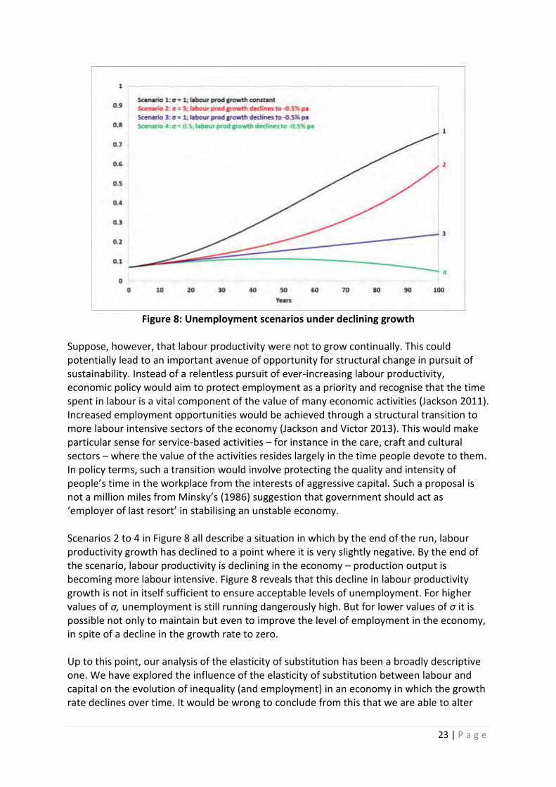
Discussion In his bestselling book, Capital in the 21st Century, French economist Thomas Piketty has proposed a simple and potentially worrying thesis. Declining growth rates, he suggests, give rise to worsening inequalities. This paper has confirmed that, under certain conditions, it is indeed possible for income inequality to rise as growth rates decline. However, we have also established that there is absolutely no inevitability at all that a declining growth rate leads to explosive (or even increasing) levels of inequality. Even under a highly-skewed initial distribution of ownership of productive assets, it is entirely possible to envisage scenarios in which incomes converge over the longer-term, with relatively modest intervention from progressive taxation policies. The most critical factor in this dynamic is the elasticity of substitution, 𝜎, between labour and capital. This parameter indicates the ease with which it is possible to substitute capital for labour in the economy as relative prices change. Higher levels of substitutability (𝜎 > 1) do indeed exhibit the kind of rapid increases in inequality predicted by Piketty, as growth rates decline. In an economy with a lower elasticity of substitution (0 < 𝜎 < 1), the dangers are much less acute. The ease with which capital can be substituted for labour is thus an indicator of the propensity for low growth environments to lead to rising inequality. More rigid capital-labour divisions on the other hand appear to reinforce our ability to reduce societal inequality. From a conventional economic viewpoint, this might appear to be cold comfort. Lower values of σ are often equated with lower levels of development. As Piketty points out (2014a: 222), low levels of elasticity characterised traditional agricultural societies. Other authors have suggested that the direction of modern development, in general, is associated with rising elasticities between labour and capital (Karagiannis et al 2005). Antony (2009a) and Palivos (2008) both argue that typical empirical values of 𝜎 are less than one for developing countries and above one for developed countries. The suggestion in the literature appears to be that progress comprises a continual shift towards higher levels of σ. But this contention embodies numerous ideological assumptions. In particular it seems to be consistent with a particular form of capitalism that has characterised the post-war period: a form of capitalism that has come under increasing scrutiny for its potent failures, not the least of which is the extent to which it has presided over continuing inequality (Davidson 2013, Galbraith 2013). The possibility of re-examining this assumption resonates strongly with suggestions in the literature for addressing the challenge of maintaining full employment under declining growth. In our own work, for example, we have responded to this challenge by highlighting the importance of labour-intensive services both in reducing material burdens across society and also in creating employment in the face of declining growth (Jackson 2009; Jackson and Victor 2011). The findings from the SIGMA model support this view. In fact, with growth and savings rates equal to those in Figure 7, initial distributions of income and capital as assumed there, and constant labour productivity growth of 1.8% per annum, unemployment rises to over 70% (Figure 8: scenario 1), a situation that would clearly be disastrous for any society.

23 | P a g e

Figure 8: Unemployment scenarios under declining growth

Suppose, however, that labour productivity were not to grow continually. This could potentially lead to an important avenue of opportunity for structural change in pursuit of sustainability. Instead of a relentless pursuit of ever-increasing labour productivity, economic policy would aim to protect employment as a priority and recognise that the time spent in labour is a vital component of the value of many economic activities (Jackson 2011). Increased employment opportunities would be achieved through a structural transition to more labour intensive sectors of the economy (Jackson and Victor 2013). This would make particular sense for service-based activities – for instance in the care, craft and cultural sectors – where the value of the activities resides largely in the time people devote to them. In policy terms, such a transition would involve protecting the quality and intensity of people’s time in the workplace from the interests of aggressive capital. Such a proposal is not a million miles from Minsky’s (1986) suggestion that government should act as ‘employer of last resort’ in stabilising an unstable economy. Scenarios 2 to 4 in Figure 8 all describe a situation in which by the end of the run, labour productivity growth has declined to a point where it is very slightly negative. By the end of the scenario, labour productivity is declining in the economy – production output is becoming more labour intensive. Figure 8 reveals that this decline in labour productivity growth is not in itself sufficient to ensure acceptable levels of unemployment. For higher values of σ, unemployment is still running dangerously high. But for lower values of σ it is possible not only to maintain but even to improve the level of employment in the economy, in spite of a decline in the growth rate to zero. Up to this point, our analysis of the elasticity of substitution has been a broadly descriptive one. We have explored the influence of the elasticity of substitution between labour and capital on the evolution of inequality (and employment) in an economy in which the growth rate declines over time. It would be wrong to conclude from this that we are able to alter

24 | P a g e

this elasticity at will. Most conventional analyses (Duffy and Papageorgiou 2000, Pereira 2003, Chirinko 2008) assume that values of σ are given – an inherent property of a particular economy or state of development. Such analyses usually confine themselves to showing how allowing for a range of elasticity facilitates a better econometric description of a particular economy than assuming an elasticity of 1. Our own analysis here also assumes that the elasticities themselves are fixed over time. The production function in equation (21) is predicated precisely on this assumption. There is however a tantalising suggestion inherent in this analysis that changing the elasticity of substitution between labour and capital offers another potential avenue towards a more sustainable macro-economy, and in particular a way of mitigating the pernicious impacts of inequality and unemployment in a low growth economy. Exploring that suggestion fully is beyond the scope of this paper, but is certainly worth flagging here. It would require us first to move beyond the CES production function formulation adopted here. The appropriate functional form for such an exercise would be a Variable Elasticity of Substitution (VES) production function. We note here that there is substantial justification and considerable precedent for such a function (Sato and Hoffman 1968, Revankar 1971). Antony (2009b) suggests that VES functions offer better descriptions of real economies than either CES or Cobb-Douglas functions. Adopting such a function would allow us to explore scenarios in which σ changes over time. An alternative approach might be to adopt an institutionalist framework such as the one proposed by Barbosa-Filho (2014). We should also recall here our assumption that the rate of return to capital is equal to the marginal productivity of capital. As we remarked earlier, this assumption only holds in markets conditions where capital is unable to use its power to command a higher share of income. Clearly, in some of the scenarios we have envisaged, this assumption may no longer hold. Where political power accumulates alongside the accumulation of capital, the danger of rising inequality is particularly severe and is no longer offset simply by changes in the economic structure. This question also warrants further analysis. In summary, this paper has explored the relationship between growth, savings and income inequality, under a variety of assumptions about the nature and structure of the economy. Our principal finding is that rising inequality is by no means inevitable, even in the context of declining growth rates. A key policy conclusion concerns the need to protect wage labour against aggressive cost-reducing strategies to favour the interests of capital. This measure would have the additional benefit of maintaining high employment, even in a low- or degrowth economy.

25 | P a g e

References D’Alisa, G, F Demaria and G Kallis (eds) 2014. Degrowth: a vocabulary for a new era. London:

Routledge. Antony, J 2009a Capital/Labor Substitution, Capital Deepening and FDI. Journal of

Macroeconomics 31 (2009) 699–707. Antony, J 2009b A Toolkit for Changing Elasticity of Substitution Production Functions. The

Hague: CPB Netherlands Bureau for Economic Policy Analysis. Arrow, K H Chenery, B Minhas and R Solow 1961. Capital-Labor Substitution and Economic

Efficiency. The Review of Economics and Statistics 43(3): 225-250. Barbosa-Filho, N 2014. Elasticity of substitution and social conflict: a structuralist note on

Piketty’s Capital in the 21st Century. Contribution to a Symposium on Thomas Piketty’s Capital in the 21st Century – a structuralist response. Online at:

http://www.economicpolicyresearch.org/images/INET_docs/publications/2014/Barbosa_paper2_PikettySymposium.pdf.

Bezemer, D 2010. Understanding financial crisis through accounting models. Accounting, Organizations and Society 35(7): 676-688.

BoE 2014. Money Creation in the Modern Economy. Bank of England Quarterly Bulletin 2014 Q1. Online at: http://www.bankofengland.co.uk/publications/Documents/quarterlybulletin/2014/qb14q1prereleasemoneycreation.pdf#page=1.

Buchanan, A 1982. Marx and Justice: the radical critique of liberalism. New Jersey: Rowman and Littlefield.

Cantore, C, P Levine, J Pearlman and B Yang 2014. CES Technology and Business Cycle Fluctuations. Discussion Papers in Economics D04/14. Guildford: University of Surrey, Economics Department.

Chirinko, R 2008. σ: the long and short of it. Journal of Macroeconomics 30: 671–686. Cohen, A. and G Harcourt 2003. Retrospectives: Whatever Happened to the Cambridge

Capital Theory Controversies?. Journal of Economic Perspectives 17 (1): 199–214. Copeland, M 1949. Social accounting for money flows. The Accounting Review 24(3): 254-

264. Daly, H 1996. Beyond Growth. Washington: Island Press. Davidson, P 2013. Income inequality and hollowing out the middle class. Journal of Post-

Keynesian Economics 36(2): 381-383. Dorman, P 2014. Macroeconomics – a fresh start. New York: Springer-Heidelberg. Duffy, J and C Papageorgiou 2000. A cross-country empirical investigation of the aggregate

production function specification. Journal of Economic Growth 5: 87–120. Galbraith, J 2013. The Third Crisis in Economics. Journal of Economic Issues 47(2): 311-322. Giddens, A 1995. A Contemporary Critique of Historical Materialism. Stanford: Stanford

University Press. Godley, W 1999. Seven Unsustainable Processes: medium term prospects for the US and for

the world. NY: Levy Economics Institute. Online at: http://www.levyinstitute.org/pubs/sevenproc.pdf.

Godley, W and Lavoie, M 2007. Monetary Economics – An Integrated Approach to Credit, Money, Income, Production and Wealth. London: Palgrave Macmillan.

Goodwin, R 1967. Socialism, Capitalism and Growth. Cambridge: Cambridge University Press.

26 | P a g e

Gordon, R 2012. Is US economic growth over? Faltering innovation confronts the six headwinds. National Bureau of Economic Research Working Paper 18315. Cambridge, Mass: NBER. Online at: http://www.nber.org/papers/w18315 (accessed 20th October 2014).

Jackson, T 2009. Prosperity without Growth – economics for a finite planet. London: Routledge.

Jackson, T 2011. Let’s be less productive. Opinion piece. New York Times 26th May 2012. Online at: http://www.nytimes.com/2012/05/27/opinion/sunday/lets-be-less-productive.html?_r=0.

Jackson, T and P Victor 2011. Productivity and Work in the New Economy – Some Theoretical Reflections and Empirical Tests, Environmental Innovation and Societal Transitions, Vol.1, No.1, 101-108.

Jackson, T and P Victor 2013. Green Economy at Community Scale. A report to the Metcalf Foundation. Toronto: Metcalf Foundation. Online at: http://metcalffoundation.com/wp-content/uploads/2013/10/GreenEconomy.pdf.

Jackson, T and P Victor 2014. Does slow growth increase inequality? Some reflections on Piketty’s ‘fundamental laws of capitalism’. PASSAGE Working Paper 14/01. Guildford: University of Surrey.

Jackson, T and P Victor 2015. Stock-Flow Consistency and Ecological Macro-Economics, PASSAGE working paper 15/01. Guildford: University of Surrey.

Jackson, T, B Drake, P Victor, K Kratena and M Sommer 2014. Literature Review and Model Development. Workpackage 205, Milestone 28, Wealth, Welfare and Work for Europe. Vienna: WIFO.

Howard, R and Kennedy 2015. Economic Growth, Inequality and Well-Being. Ecological Economics: this volume.

Kaldor, N 1955. Alternative Theories of Distribution. The Review of Economic Studies 23(2): 83-100

Kalecki, M 1939. Essays in the Theory of Economic Fluctuations. Kallis, G, C Kerschner, and J Martinez-Alier 2012. The economics of degrowth, Ecological

Economics 84:172-180. Karagiannis, G, T Palivos and C Papageorgiou 2005. Variable Elasticity of Substitution and

Economic Growth: Theory and Evidence. In C Diebolt and C Kyrtsou Eds) New Trends in Macroeconomics. New York: Springer.

Krusell P and A Smith 2014. Is Piketty’s ‘Second Law of Capitalism’ fundamental? Working Paper (1st Version). Washington DC: National Bureau of Economic Research.

Latouche S 2007. De-growth: an electoral stake? International Journal of Inclusive Democracy 3(1). Online at: http://www.inclusivedemocracy.org/journal/vol3/vol3_no1_Latouche_degrowth.htm.

MGI 2015. Global growth: can productivity save the day? New York: McKinsey Global Institute. Online at: http://www.mckinsey.com/insights/growth/can_long-term_global_growth_be_saved?cid=other-eml-nsl-mip-mck-oth-1502.

Minsky, H 1986. Stabilizing an Unstable Economy. New Haven: Yale University Press. OECD 2014 Policy challenges for the next fifty years. OECD Economic Policy Paper No 9, July

2014. Paris: OECD. ONS 2014. Wealth and Income 2010-2012. Statistical Bulletin. Office for National Statistics.

Online at: http://www.ons.gov.uk/ons/dcp171778_368612.pdf.

27 | P a g e

Oxfam 2015. Wealth: having it all and wanting more. Oxford: OXFAM. Online at: http://policy-practice.oxfam.org.uk/publications/wealth-having-it-all-and-wanting-more-338125.

Palivos, T 2008. Comment on σ: the long and short of it. Journal of Macroeconomics 30: 687–690.

Papathanasopoulou, E and T Jackson 2009. Measuring fossil resource inequality – a case study for the UK between 1968 and 2000. Ecological Economics 68: 1213 – 1225.

Pereira, C 2003. Empirical Essays on the Elasticity of Substitution, Technical Change, and Economic Growth. North Carolina State University. Online at: http://repository.lib.ncsu.edu/ir/bitstream/1840.16/4460/1/etd.pdf.

Piketty, T 2014. Capital in the 21st Century. Cambridge, Mass: Harvard University Press. Piketty, T 2010. On the Long-Run Evolution of Inheritance: France 1820-2050. Paris: Paris

School of Economics, Working Paper. Piketty, T and G Zucman. 2013. Capital is Back: Wealth-Income Ratios in Rich Countries

1700-2010. Paris: École d’Économie de Paris. Revankar, N 1971. A Class of Variable Elasticity of Substitution Production Functions.

Econometrica 39(1): 61-71. Rezai, A, L Taylor and R Mechler. 2013. Ecological Macroeconomics: An application to

climate change. Ecological Economics 85: 69-76. Robinson, J 1953. The Production Function and the Theory of Capital. Review of Economic

Studies 21: 81. Saez E and G Zucman 2014. Wealth Inequality in the United States since 1913: Evidence

from Capitalized Income Tax Data. Cambridge, Mass: National Bureau of Economic Research. Online at: http://gabriel-zucman.eu/files/SaezZucman2014.pdf.

Sato R and R Hoffman 1968. Production Functions with Variable Elasticity of Factor Substitution: Some Analysis and Testing. Rev Econ and Stats 50(4): 453-460.

Stiglitz, J, A Sen and P Fitoussi 2009. Report of the Commission on the Measurement of Economic Performance and Social Progress. Online at: http://www.stiglitz-sen-fitoussi.fr/documents/rapport_anglais.pdf (Accessed 22nd October 2014).

Stymne, S and T Jackson 2000. Intra-generational equity and sustainable welfare: a time series analysis for the UK and Sweden. Ecological Economics 33: 219–236.

Victor, P 2008. Managing without growth - slower by design, not by disaster. Cheltenham: Edward Elgar.

Wolff, E and A Zacharias 2007. Class Structure and Economic Inequality. Levy Economic Institute Working Paper No 487. NY: Levy Economics Institute. Online at: http://www.levyinstitute.org/pubs/wp_487.pdf.

28 | P a g e