Does Tallness Pay Off in the Long Run?

Height and Life-Cycle Earnings

Elisabeth Lång∗, Paul Nystedt†#

December 4, 2014

Abstract

The existence of a height premium in earnings is well documented, but how it develops over the life cycle is largely unknown. By using data on approximately 43,500 dizygotic and monozygotic twins born in Sweden 1889-1958, we analyze how the height premium in earnings changes over the adult lifespan. OLS regression estimation of the height premium reveals that one decimeter additional height is associated with, on average, 6-10 percent greater earnings. Moreover, the height premium increases over the life cycle for men, but decreases for women. Within twin-pair fixed effects (WTP) estimates are on average about 40 percent lower than the OLS estimates for men, suggesting that genetic endowments and early life environmental conditions operating on a family level explain a significant part of the unconditional returns to tallness throughout adult life. Including education as an explanatory variable induces a similar reduction (about 40 percent) of the estimated OLS height premium, but has no effect whatsoever on the within twin pair estimates, implying that the OLS and WTP estimates tend to coincide. Hence, it seems as if schooling may mediate the association between height and earnings among unrelated male individuals but not among twins. For women, the differences between the OLS and WTP estimations are less precise.

∗ Linköping University

���† Jönköping International Business School # Jönköping Academy for Improvement of Health and Welfare

1

1 Introduction The association between height and labor market outcomes such as earnings is well

known. Scholars from various disciplines have explored this topic for at least 100 years,

documenting a strong positive relationship between adult stature and earnings by employing a

variety of data sources, reaching from historical data from the 18th and 19th centuries (e.g.,

Jacobs and Tassenaar, 2004; Komlos, 1990) to more recent data from developing countries

(e.g., Steckel, 1995; Thomas and Strauss, 1997) as well as modern societies (e.g., Case and

Paxson, 2008; Case et al., 2009; Lundborg et al., 2014; Persico et al., 2004).1

Recent research suggests that in the contemporary western world (e.g., USA, Great

Britain and Sweden) the average increase in earnings resulting from being 10 centimeters

taller is substantial, similar in magnitude to one additional year of schooling (i.e. about 10

percent in the United States and United Kingdom, and about 6 percent in Sweden, Card, 1999;

Case and Paxson, 2008; Lundborg et al., 2014; Persico et al., 2005). The height premium has

been attributed to stature being associated with productivity related characteristics in the form

of non-cognitive (social) skills (Persico et al. 2005) and cognitive skill (Case and Paxson

2008), or both (Lundborg et al. 2014, Schick and Steckel 2010).

Previous studies on height and earnings are mainly based on cross-sectional analysis of

fairly young people (aged 30-40) and it is still not known how the height premium develops

over the life cycle. Moreover, in analysis on unrelated individuals it is uncertain to what

extent unobserved individual or family environmental or genetic characteristics influence the

estimated relationships. Lundborg et al. (2014) neutralizes some of this by studying variation

between brothers who share family environment and, on average, 50 percent of their genes.

Though two brothers share some genes and early-life environmental conditions, they differ in

birth parity implying that one of them grew up with an older brother and the other with a

younger brother. Furthermore, family conditions are generally not static, which means that

siblings may face similar conditions at the same point in time but not necessarily at the same

age. This may be important if family conditions change over time and environmental

influences (or gene-environment interactions) are age sensitive.

The purpose of this paper is to analyze the development of the returns to tallness over

the adult lifespan, for both men and women, and to investigate to what extent unobserved 1 See also: Gowin (1915); Hamermesh and Biddle (1994); Persico, Postlewaite, and Silverman (2004); Steckel (2009).

2

early life environmental conditions and genetic endowments influence the crude (or

unconditional) height premium from this respect. To analyze the association between height

and earnings we utilize longitudinal annual register data on earnings 1968-2007 for 21,740

same sex twin pairs from the Swedish Twin Registry, born 1889-1958. We follow these twins

from early adulthood (age 25) to old age (79) in order to establish how the return to tallness is

developing over the entire labor market career and in retirement age.2 By also studying the

development of the height premium over the life cycle for consecutive birth cohorts, we

address whether it has changed over time for different age groups. A twin differencing design

is employed in order to provide new evidence on the association between height and earnings.

Under the assumption that the height variation among MZ twins is environmentally induced

(i.e. depends on, for example, accidents and diseases striking unevenly between the twins

during childhood and youth), whereas the corresponding variation among DZ twins could be

of either genetic or environmental (or both) origin, a comparison of the height premium in

respective sample will indicate the relative importance of environmentally and genetically

induced variations in height for earnings.

We find that taller people earn more: one decimeter additional height is associated with

about 6-10 percent greater earnings, a magnitude similar to the findings of previous studies

(see Section 2 for further discussion). Whereas the height premium increases with age for

men, it decreases for women. Analysis on three consecutive birth cohorts reveals that the

height premiums have declined somewhat over time. Within twin-pair fixed effects (WTP),

analysis reveals that, for men, about 30-40 percent of the crude height premium is explained

by unobserved factors shared by twins. There is just a slight and imprecisely measured

difference between DZ and MZ twins from this respect, suggesting that the main origin of the

height variation (i.e. whether of genetic or environmental character) does not seem to severely

influence the magnitude of the height premium for men. For women, it seems as if the height

premium generally is somewhat lower when restricting the sample to MZ twin pairs, though

the resulting age patterns are less stable.

The rest of the article is organized as follows. In Section 2 we review literature that is

related to our study and discuss determinants of height and the association between height and

earnings. We present the empirical framework of our study, and descriptions of the variables

2 Note that we obviously cannot follow the same individuals over the entire age span considered in the main analysis (25-79), since data on earnings are only available from 1968 (when the oldest individuals born 1889 were 79 years old) to 2007 (when the youngest individuals born 1958 were 49 years old).

3

used in the analyses in Section 3. Descriptive statistics, the main results of our study, and

sensitivity analyses are presented in Section 4. Section 5 provides a concluding discussion.

2 Background and Previous Literature Determinants of Height

Three broadly defined mechanisms explain disparities in height growth and subsequent

variation of adult stature: heritability of height, environmental factors, and gene-environment

interactions (Silventoinen, 2003). Adult height has therefore been widely utilized as a marker of

secular trends and socioeconomic variations in childhood conditions (Silventoinen 2003; see also

the literature discussion in Section 1). Although an adult individual’s height has been denoted

“probably the best single indicator of his or her dietary and infectious disease history during

childhood” (Elo and Preston, 1992), studies have found that up to 80 percent of the variation in

height can be explained by genetic factors in modern societies (e.g., Stunkard et al. 1986;

Silventoinen et al., 2003). Apart from the aspect of genetics, environmental factors in utero,

infancy and childhood are according to the early-life hypothesis bound to affect health,

cognitive ability, human growth and stature in adulthood (e.g., Barker 2007). Silventoinen

(2003) also emphasizes the importance of nutrition and presence of diseases during the early

stages in life on adult stature.

Although a substantial fraction of the height variation in the western world could be

attributed to genetics, this is obviously not the case for height differences between MZ twins.

Since MZ twins share genetic predispositions, height variations between them are bound to be

environmentally induced. From this perspective, such variations constitute a window of

observation into environmental conditions striking unevenly between the twins. It does not

seem farfetched to suggest that these are more likely to be a result of exogenous variation (i.e.

placement in the womb, accidents and illnesses) than to any systematic discrimination by

parents favoring one of the twins. However, parents may adapt to variation in inherent

capabilities or random insults striking unevenly among their children by compensatory (or

reinforcing) measures, i.e. investing more (or less) time and money in the less (more)

fortunate child. In such case, the pure impact of these insults will be counteracted (or

reinforced) by parental behavior. While some empirical twin-based studies, using various

measures of parental inputs, do not suggest that parents systematically reinforce or

compensate for early life insults (see for instance Royer, 2009; Almond and Currie, 2011),

4

there are some evidence on the contrary presented on US data (compensatory, Lundborg,

2013) and China (reinforcing, Rosenzweig and Zhang, 2009).

Height and Earnings

The empirical evidence on variations in adult height and its return in the labor market

has revealed that being taller is associated with having higher earnings. How this premium

arises is yet not fully understood, even less is known about how it develops over the life cycle

and whether it has changed over time. One conjecture is that there is a general preference for

tallness in the society, implying that tall people are positively discriminated, or vice versa,

short people negatively discriminated against. This means that, regardless of their actual

productivity capabilities, people are to some extent paid according to their height. A second

proposition is that stature is associated with certain productivity related traits that are valued

and rewarded on the labor market. Such associations may in turn arise from height affecting

the development of such characteristics. This is a main feature in the argumentation of Persico

et al. (2005), which, by studying the hourly wage rate at age 33 in the British National Child

Development Study (NCDS) and for people aged 31-38 in the U.S. National Longitudinal

Survey of Youth (NLSY), find that the height premium is reduced when non-cognitive skills

is included as an explanatory variable. They put forth that height during youth promotes

participation in sport and social college clubs facilitating the formation of non-cognitive

(social) skills. If this argument is correct, there is a causal link from height to earnings via

mediation of this type of skills.

It could, however, also be that there is some underlying third factor governing height as

well as earnings. This would be the case if height growth and cognitive development, which is

likely to be valued on the labor market, both are subject to common genetic or environmental

developmental mechanisms in the form of e.g. insulin-like growth factors. Twin-based studies

suggest that this is indeed the case (Silventoinen et al. 2003; Sundet et al. 2005). The overall

association between height and cognition has mainly been attributed to genetic inheritance

and shared environmental factors operating at a family level (the relative importance of the

former being emphasized when assortative mating is taken into account, and plausibly also

when there is less variation in income and nutritional conditions between families in society),

and to a lesser extent to non-shared environmental effects (Beauchamp et al. 2011, Keller et al.

2013). Case and Paxson (2008), studying the US National Child Development Study (NCDS)

data set and data from the British Cohort Study (BCS), find that a large portion of the crude

height premium in earnings among unrelated individuals measured at age 30 (BCS) and 33 or

5

42 (NCDS) is explained by variation in cognitive skills.3 Lundborg et al. (2014) analyzes

180,000 Swedish male brothers 28-38 years old in a sibling fixed-effects framework and find

that cognitive and non-cognitive skills as well as unobserved factors operating at the family

level explain the lion’s share of the crude association between height and earnings. Notably, a

statistically significant height premium still remains once these factors are controlled for.

Closer inspection reveals that this remaining height premium is concentrated to the lower end

of the height distribution, indicating that discrimination may occur among short (but not tall)

people. In recent research, Böckerman and Vainiomäki (2013) analyze the height premium of

average earnings 1990-2004 among 10,000 Finnish MZ twins born 1944-1958. Exploiting

within twin differences in self-reported height, they find a statistically significant premium

among female twins but not for male twins.4

3 Method ��� and Data 3.1 A Simple Model of Height and Earnings To form a basis for the analysis of the height premium in earnings we employ a simple

conceptual, counterfactual framework:5

𝜉!,! ≡ 𝜙!,! ℎ [1]

where 𝜉!,! represents the potential earnings of individual I at age A, and h represents adult

height. In this setting, the earnings of an individual depend on his or her stature, holding other

characteristics constant. In other words, 𝜙!,!! ℎ measures the height premium in earnings at a

given age.

A statistical extension of the deterministic model [1] is:

𝑦!,! = 𝛼! + 𝛽!ℎ! + 𝑋!𝛾 + 𝑍!𝛿 + 𝜇! + 𝜀!,! [2]

where the subscript i refers to individual i, y is earnings, h is adult height, and X is a vector of

individual control variables, Z is a vector of environmental and social family background

3 Schick and Steckel (2010), also studying the NCDS, show that cognitive and noncognitive skills explain equal parts of the unconditional height- earnings association. 4 In an attempt to avoid potential measurement error problems, they also estimate a model where self-reported height in one period is instrumented by self-reported height in another period (under the assumption that measurement errors in height are classical and non-correlated within the twin pair). This inflates the height premium so that the WTP estimates exceeds the crude OLS estimates by almost 300 and 700 percent for men and women, respectively. 5 This framework is similar to the one formulated in Lundborg et al. (2014).

6

variables that are fixed in adult life, and 𝜇 represents heritable traits, all of which are affecting

earnings.6 If the entire vector X, Z, and 𝜇 are observable the estimate of 𝛽 will measure the

height premium in earnings of being one unit of length taller.

3.2 Empirical Framework

When estimating the height premium empirically, model [2] will ideally capture the

causal effect on earnings of being taller. Estimating model [2] by using OLS regression

methods is, however, likely to create problems of inference because of unobservable factors,

resulting in omitted variable bias. If, for instance, unobserved background factors

simultaneously governs height and cognition (which is also unobserved), creating a positive

association between the two – and the latter also influence earning, OLS of height on earnings

will result in biased estimates of the height premium. Insofar such background factors are

shared between two study subjects (for example twins), differencing between them will

neutralize such bias. Hence, the WTP specification is employed, cancelling out the effects of

shared family environmental conditions and genetic inheritance.

Consider model [2] for twin i and j in a pair of (same gender) twins and take the first

difference of these two equations:

𝑦!",! − 𝑦!",! = 𝛽!(ℎ!" − ℎ!")+ (𝑋!" − 𝑋!")𝛾 + (𝑍!" − 𝑍!")𝛿 + (𝜇!" − 𝜇!")+ (𝜀!" − 𝜀!") [3]

where the subscript s refers to a given pair of twins (s=1,2,…,n). Assuming that two twins

within a pair share the same family background, the Z vector cancels out. If genetic heritable

traits are fully shared between two twins within a pair (as for MZ twins), 𝜇 cancels out as well.

Hence the model becomes:

∆𝑦!,! = 𝛽!∆ℎ! + ∆𝑋!𝛾 + 𝑣! [4]

where Δ represents the first difference between twin i and j for each given twin pair s and 𝑣!

represents the first difference in the error.

Albeit utilizing specification [4] will, at least partly, overcome the issue of omitted

variable bias discussed in the text above, it will not tell us if the estimated effect is stationary

or if the height premium in earnings changes over the life cycle. Therefore equation [4] will

be estimated for eleven consecutive 5-year windows of age (age waves) ranging from 25-29

to 75-79. In our base case scenario we will assume that the entire X vector will be neutralized 6For ease of exposition, it is implicitly assumed that the effects of X, Z and 𝜇 are constant over age in this specification.

7

when applying the within twin-pair difference approach.7 Differencing between twins, all

unobserved factors common to the twins within a pair cancel out. This implies that

identification of the regression coefficients in WTP models is obtained solely via within twin-

pair variation in the covariates.8

To fully capture causal effects of interest, the variation in explanatory variables between

twins has to be truly exogenous. In many twin based studies (on, for example, the effects of

education on income), environmentally induced within twin pairs differences pose a threat as,

ideally, the twins should be equal in all (unobserved) respects in order to establish a causal

relationship. It is therefore often implicitly assumed that twins during their childhood fully

share the same environmental conditions. Contrary to such studies, the fundaments of our

study rely explicitly and ultimately on exogenous variation in the early life and childhood

environment conditions, even within MZ twin pairs, resulting in height variations among

them. Given that MZ twins share genetic predispositions, and height growth is a function of

such predispositions, environmental conditions and their interaction, any variation in stature

between them is bound to be a function of variation in their environment. Such variations

occur from conception onwards and twins do differ in outcomes very early in life such as

birth weight. In the case of MZ twins, the height premium could thus be traced back solely to

non-shared environmental factors. Hence, comparing the results obtained in the DZ twin-pair

and the MZ twin-pair cases will give indications of whether height differences induced solely

through environmental variations (MZ twin-pair differences) and those also induced by

genetic differences (DZ twin-pair differences) are associated with similar height premiums.

The twin design brings certain distinct advantages to the analysis of the relation

between height and earnings. It enables analysis of variables that are constant over time (such

as height), which is unfeasible in traditional fixed effects panel data models based on repeated

individual observations (see for example Wildman 2003; Islam et al 2010). Identification

based on twin differencing is obtained via variation within twin pairs, and in the present case

virtually all twins have different earnings (and adult height). It should also be noted that twin

estimates are likely to reflect a population average of the considered effects, as differences

7 In order account for plausible time effects, we also include birth year fixed effects in all OLS regression specifications. 8 In the main specification we will only include height as an explanatory variable. Variables such as years of schooling and birth weight are not included as the effects of height on earnings may well be mediated through them. To analyze the extent to which the height premium is affected by inclusion of such variables in the specification, we also perform several sensitivity analyses in which we include different covariates (see Section 4.2).

8

within twin pairs in for example height are likely to be represented along the entire height

distribution.

3.3 Data

Our main data on height is from the Swedish Twin Registry (STR), managed by the

Karolinska Institute in Stockholm, Sweden. The STR was established in the 1960s and is the

largest of its kind to this date. The registry holds information on about 85,000 pairs of twins

born in Sweden since 1886. The STR defines zygosity status of pairs of twins based on

questions of intrapair similarities in childhood, a method that studies using DNA validation

have shown to have approximately 98 percent accuracy (see Lichtenstein et al., 2002, for a

comprehensive description of STR). The sample used in this paper includes only twin pairs

with known zygosity, DZ or MZ. By the use of personal identification numbers we merge the

STR height data with information on earnings. Below follows a brief description of the main

variables utilized in this study.

Adult Height

Height is self-reported in questionnaires from 1963, 1970, 1973 and 1998-2002. In

order to obtain an appropriate measure of adult height we have followed a procedure where

we, for each and every twin pair, use the information in the first available questionnaire where

the twin couple is at least 18 years old and they both have answered it. Such a procedure will

make sure that the reported height reflects adult height and that it is reported for the same age

of both twins within a pair.9

Since height is self-reported, there is an issue of possible measurement errors in the

explanatory variable. Under the classical errors in variables (CEV), OLS regression estimates

will be biased and inconsistent; in within fixed effects models, such as sibling and twin

models, the problem of CEV will be of even greater magnitude (Bound and Solon, 1999;

Griliches, 1977; Grilches, 1979; Neumark, 1999). However, an analysis by Dahl et al. (2010),

based on a subsample of the STR twins, some of which are followed under a period of 20

years, shows that misclassification in self-reported height is rather small. In their first

investigation wave, when the twins already were rather old (mean age: 63.9, age range; 40-

88) the mean error in reported height was +0.9 cm. The authors also show that the

misclassification increases with age (0.038 cm per year, which is less than 0.8 cm over 20

9 A handful of observations pertaining to reported height above 250 and below 100 cm were excluded.

9

years), probably due to peoples’ self-perceived body image not fully adapting to the fact that,

after the age of 40, they tend to shrink slightly, by about 0-5-1 cm per decade for men and

about 1-2 cm for women, respectively. From this perspective it should be noted that we

control for annual birth cohort in every OLS regression in order to found our height premium

parameter estimates on intra-cohort height variations (rather than age variations due to trends

in height growth or age related decreases in height). Especially Swedish males under the age

of 40 in the birth cohorts who underwent mandatory enlistment (born before 1978) where

height was measured, have a highly valid perception of their height. Moreover, it seems

highly plausible that measurement errors in self-reported height within twin pairs are

positively correlated since they ought to share several characteristics due to their common

genetic and environmental inheritance; they are always in the same age, ought to shrink in

similar pace and be similarly inclined to update their body image according to changes herein,

et cetera. Taken together, this suggests that WTP differences in height should be less plagued

by the problem of measurement errors than if such errors were randomly distributed between

the twins in accordance with CEV. Unfortunately we do not have data on measurement errors

in height and thus cannot make a direct and absolute assessment of the potential problem of

CEV. Nevertheless, we will assess the potential importance of measurement error in height

indirectly by using correlations and variances based on the self-reported height measure (see

Appendix).

Earnings

Data on earnings is provided by Statistics Sweden and given by individual earned

taxable income 1968-2007. The consumer price index has been used to deflate income across

the years to the price level of 2010. Annual income is expected to carry small measurement

errors, since the data is obtained from registers. Income was then aggregated into 5-year

averages for every individual according to age ranging from 25-29 to 75-79, resulting in

eleven consecutive measures. In our empirical specification we will use logarithm of earnings,

implying that a portion of the sample will be dropped due to zero income. It should also be

noted that earned taxable income includes income from employment, self-employment,

parental-leave benefits, unemployment insurance, and sickness-leave benefits (these sources

of income are also included in the earnings measure analyzed in the articles by Lundborg et al.

2014, and by Böhlmark and Lindqvist, 2006). Hence, our earnings measure captures

consumption boundaries rather than pure labor market productivity. Including the last three of

these income sources also serves the purpose of smoothing temporary earnings shifts. In a

10

sensitivity analysis, Lundborg et al (2014) showed that the inclusion of such benefits does not

affect the estimated height premiums for men in their thirties. Note that the effective age of

retirement in Sweden, ranging from 63 to 66 years 1976-2007 (OECD, 2014) is much lower

than the right end point of the studied age span. This implies that the estimated height

premium in earnings for the last age groups (65-69, 70-74, 75-79) in essence will capture how

height related labor market activity spills over on retirement via earned pension system

benefits.

Since the data on earnings covers a time period of 40 years, it is inevitable that there

have been some changes in the tax and social security system rules. The most extensive

reform period from this respect occurred 1973-1974 during an expansion of the social security

system when the reimbursement levels of unemployment, sickness and parental leave benefits,

all based on current and/or previous work experience and income, were increased and became

taxable. This implies that the more limited support given 1968-1972/1973 is not captured in

our earnings data. However, the influence of this should be dampened in a twin difference

setting, since income data on two twins are always taken simultaneously. Finally, the earnings

are winsorized at the 1st and the 99th percentiles in all our specifications in order to neutralize

the potential influence of extreme outliers.10

Birth Weight and Height

Data on birth weight and height is obtained from the STR BIRTH study, which is

available for twins born between 1925 and 1958 and taken from the birth records. Due to the

sampling scheme, the birth weight and height information is only available for twins that

survived until 1972. For the full sample used in the main analysis, we have access to 22,762

observations on birth weight and 22,582 on birth height. The average within twin pair

difference in birth height is about 1.5 cm, and the variation in birth weight ranges from about

300 grams (MZ twins) to about 350 grams (DZ twins), (see Table 1).

Educational Attainment

The education variable originates from several sources. For twins still alive in 1990, it is

based on register data collected by Statistics Sweden from the educational institutions in

Sweden 1990 and 2007. As for the earnings data, this implies that there should be only small

or no measurement errors. Self-reported education is provided in several of the questionnaire

waves, the first conducted in 1961, which means that we have access to information on 10 We also employ winsorized earnings at the 5th and 95th percentiles in a sensitivity analysis, with no significant changes in the height premium estimates. Results available upon request.

11

education also for people in early cohorts. The data have also been linked to self-reported

census information from 1960 and 1970, which contains a higher level of detail compared to

the survey in 1961. The education measure used is years of schooling. Average years of

schooling is about 9.5 years and the mean difference in schooling ranges from 1.3 (MZ

females) to 1.9 (DZ males) (see Table 1). About half of the twin pairs have the same

schooling, (not shown).

4 Results 4.1 Descriptive Statistics The full sample used in the main analysis contains observations on 26,834 DZ twins and

16,646 MZ twins, of which 46 percent are males and 54 percent females. Descriptive statistics

of height, within twin pair height differences, years of schooling, average annual earnings at

age 30-39, and birth weight, and height are presented in Table 1.11 Average height is similar

across zygosity, men being 10 cm taller than women. Average earnings at age 30-39 follow a

similar pattern across zygosity and men having higher earnings. The average height difference

between twins is about 5 cm for DZ and slightly more than 2 cm for MZ twins. The

distribution of height differences between twins within a pair is illustrated in Figure 1.12

The data set at hand is rich since it covers information on several birth cohorts reaching

all the way back to the end of the 19th century, but these cohorts may differ in variables that

have been shown to change over time (such as educational attainment). Therefore we also

present descriptive statistics of height, within twin pair height differences, and years of

schooling for the three different birth cohorts: those born 1900-1919, 1920-1939, and 1940-

1958.13 In Table 2 we see that height has increased over time, about 2.5-3 centimeters per

cohort. The reported height of the male twins rather well matches the average stature

registered by the enlistment authorities for the respective cohorts (Statistics Sweden, 1969).

For the cohorts enlisting 1921-1925 to 1936-1940 the average height of Swedish conscripts

11 We include descriptive statistics of average annual earnings at age 30-39 to enable comparison to previous literature, since many of these use data on people of this age. We also perform a brief analysis of earnings at age 30-39 in Section 4.2. 12 In order to make sure that our main results are not driven by extreme outliers in height differences, we perform several sensitivity analyses in which we only include pairs of twins of which the height difference between the twins are restricted to various boundaries. These sensitivity analysis results do not differ significantly from our main results. Results available upon request. 13 These birth cohorts will also be examined further in Section 4.2 in order to detect plausible time trends in the height premiums of males and females.

12

rose from 172.1 to 174.2, whereas in the twin sample the reported mean height for the first

cohort is 173.3 and 173.1 for DZ and MZ twins respectively.14 For the second cohort the

reported height is 175.6 and 175.1 (DZ, MZ) whereas the conscript mean height records

increases from 174.5 to 176.1 between 1941-1945 to 1956-1960. The corresponding figures

for the third cohort is 178.8 and 178.4 while the conscript records increases from 177.4 to 179

cm between 1961-1965 to 1977. The within twin pair differences in height and the hereto-

related standard deviations seem to be rather constant over the cohorts and thereby also with

age as later cohorts have their height reported at a younger age. Educational attainment has

increased from about 7 to more than 11 years over the cohorts under study.

Average annual earnings for the eleven age waves by zygosity and gender are shown in

Figure 2. As can be seen, average earnings of men are 50-100 percent larger than the average

earnings of women throughout the life cycle. Moreover, earnings are increasing at the

beginning of the adult life, reaching its peak at around the age of 50, to finally decrease and

level off at older ages for both genders. It is also clear that the DZ twin-pair sample and the

MZ twin-pair sample have approximately the same earnings profiles and levels throughout the

life cycle. Figure 3 and 4 illustrates the average earnings by height for different age groups for

men and women respectively. Average earnings tend to be increasing with height for both

genders, although the relationship is weak for males at the youngest age wave 25-29 years.

Though this relationship may also capture possible time trend effects, there seems to be a

positive correlation between average earnings and height.

4.2 Results

The Height Premium at Age 30-39

In order to make comparisons with previous literature possible, since most height

premiums are estimated for individuals aged 30-40, and thus strengthen the external validity

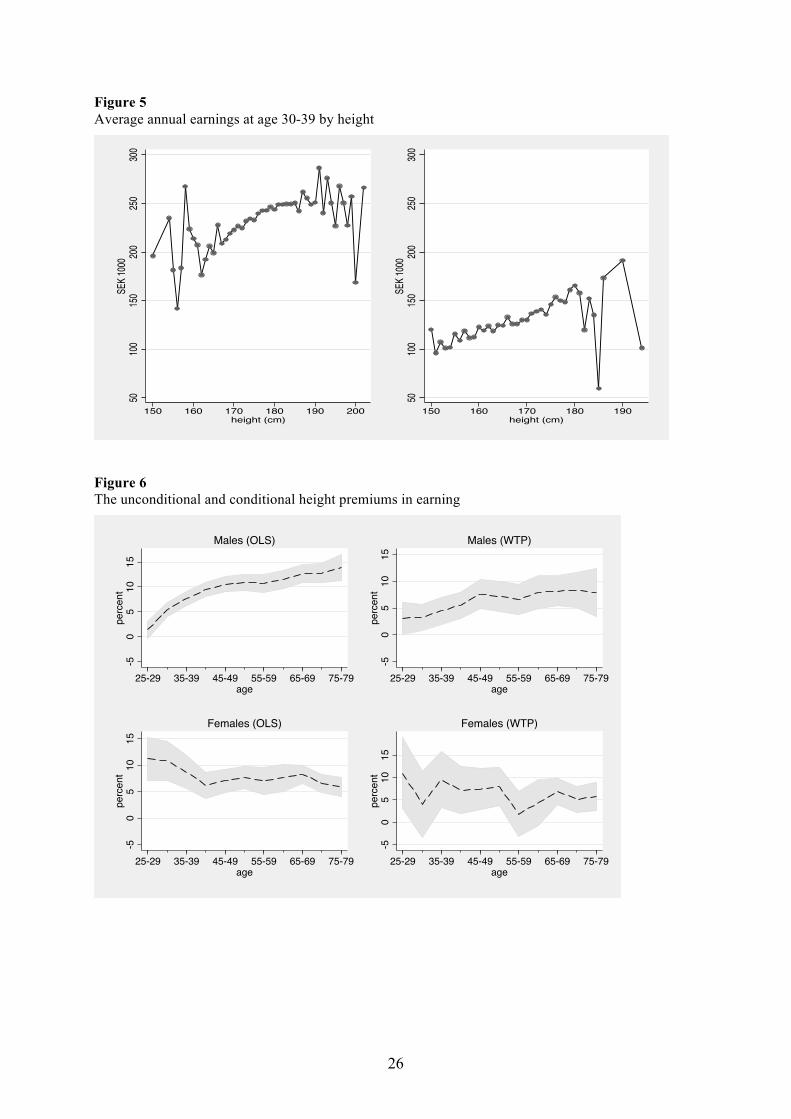
of our study, we start with examining the height premium at age 30-39. As illustrated by

Figure 5, there is a positive relationship between average earnings at age 30-39 and tallness

for both genders. This association is further examined by OLS regression and WTP regression

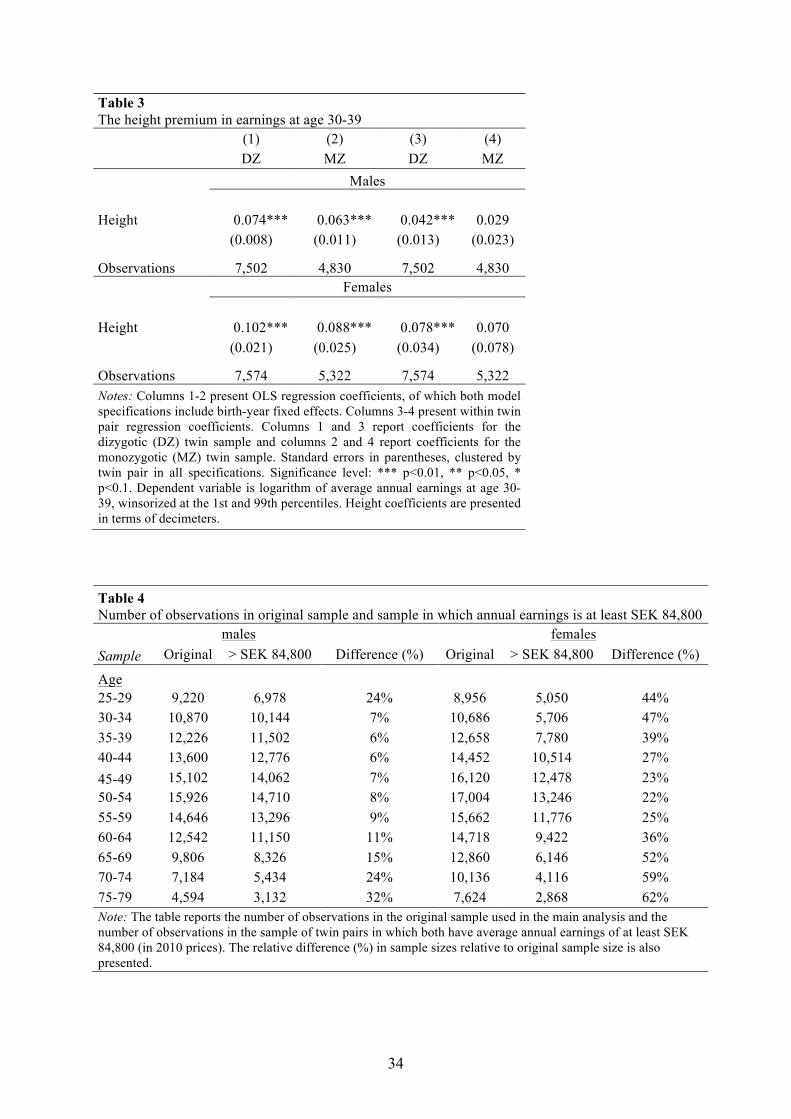
analyses. As presented by Table 3, the OLS coefficients for males are 6.3 (MZ) and 7.4 (DZ)

percent per decimeter in height. This is very similar to the estimates obtained by Lundborg et

al. (2014) for Swedish males aged 28-38. By OLS regression estimation on 448,702

individuals they uncover that being 10 centimeters taller is associated with 6.2 percent higher 14 Age of enlistment was 20 years 1915-1948. 1950-1953 it was 19 years and 1955-1967 it was 18 years.

13

earnings. By applying a within sibling specification they get a height premium of 4.2 percent,

which is equivalent to our WTP height coefficient for the DZ twin-pair sample (see Table 3).

Hence, the associations between height and earnings obtained via differencing between

brothers (who are not MZ twins) are similar in the twin sample using self-reported height

compared to the representative sample analyzed by Lundborg et al. (2014), where height was

administratively recorded by military personnel. The similarity in results indicates that

measurement errors in height are not heavily influencing the estimations of the present study.

WTP regression analysis of the MZ twin-pair sample reduces the height coefficient on

earnings to 2.9 percent and also makes it insignificant. From this it appears that more than

half of the crude height premium at age 30-39 for men can be explained by early life

environmental conditions and genetic predispositions.

The unconditional height premium for women aged 30-39 is 8.8-10.2 percent and the

conditional is about 7.8 percent, both of which are higher than the height coefficients for men.

Restricting the sample to MZ twin pairs, the WTP estimates are just slightly reduced, but

become statistically insignificant.

The Height Premium Over the Life Cycle

Having established a positive relationship between height and earnings at age 30-39, we

now turn to the main focus of this paper: the analysis of the returns to tallness over the life

cycle. The standard OLS regression and the WTP estimations of the height premium for the

pooled sample (DZ and MZ twins) are illustrated in Figure 6 (see also table A.1).15 16 As

shown, the unconditional height premium estimate is insignificant for earnings at age 25-29

for males. This is not surprising since this category may not yet have reached their earnings

potential and some of them may well still undergo further education. From age 30-34 onward,

the height premium is increasing over the life cycle for men, starting out with 5.5 percent

higher earnings to reach a magnitude of 13.9 percent higher earnings at age 75-79.

Differencing between twins lowers these height coefficients by around 30-40 percent. A

significant part of the crude height premium for men can thus be explained by unobserved

factors operating at the twin level. Moreover, the gap between the unconditional and the

conditional height premiums increases as the men grow older.

15 Height coefficients with standard errors clustered by twin pair are also presented in Table A.1 in Appendix. 16 Here we pool the sample and thus do not separate between DZ and MZ twins (as we do in later analyses). OLS regression estimations of the height premium for separate analyses on DZ and MZ twin pairs are performed, with very similar outcomes. Results available upon request.

14

Close to the opposite trend is found for women. Being 10 centimeter taller is associated

with an 11.2 percent increase in earnings for women aged 25-29. As the women grow older,

the height premium decreases and levels off to about 6 percent at age 70-79. Apart from the

age waves 30-34 and 55-59, WTP estimation does not alter the height coefficients to any

major extent, although the confidence intervals get significantly wider. The reason to why the

height coefficient dips at age 30-34 and 55-59 may be explained by labor market participation

choices among the women in our sample. This is investigated further in a sensitivity analysis

presented below.

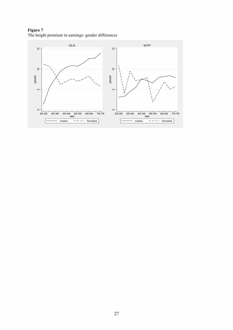
Taken together, apart from the dips in the WTP estimates at age 30-34 and 55-59, the

male and female height premium patterns form a rather symmetric scissor like shape where

the increase in the male premium is mirrored by a corresponding decrease in the female

premium, as illustrated by Figure 7. It appears as that in the long run, tallness is of more

importance for determining earnings for men than it is for women. Moreover, the extent of

which family background and genetics determine the returns to tallness seem to be greater for

men than for women throughout most of an individual’s adult life.

The results are hitherto based on individuals covering several generations and capture

the average height premiums in earnings for the considered age waves over a longer period of

time. Hence the estimates may conceal a plausible time trend in the returns to tallness. In

order to analyze whether the levels and development of these premiums have changed over

time we have re-estimated the unconditional as well as the conditional height premiums in

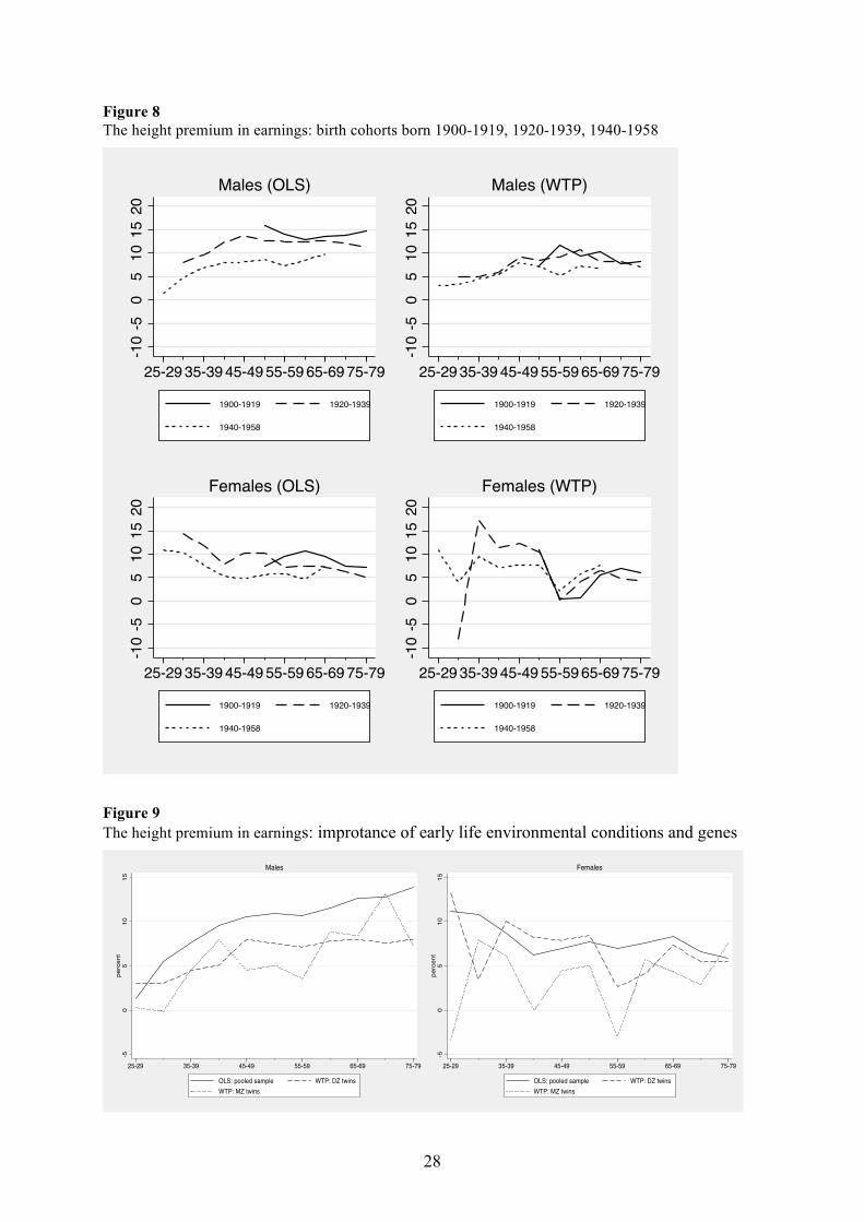
earnings for three different birth cohorts, born 1900-1919, 1920-1939, and 1940-1958 (see

table A.2-5). As shown in Figure 8, both the male and female unconditional height premiums

appear to have decreased over time for the three birth cohorts.17 Differencing between twins

gives a less clear picture; for men, it seems like the WTP height coefficients have decreased

over the cohorts studied whereas, for women, there is no apparent trend. The overall results

from cohort analysis imply that tallness has become a less important determinant of earnings.

Comparison of MZ and DZ twin pairs

Comparing OLS regression estimates with the height coefficients resulting from

differencing out endowments of early life conditions and family genetics, as we have done so

far, does not give the full picture on how important genes are for explaining the returns to

tallness. In order to separate the influences on the height premium that originates from factors

operating at the family (or DZ twin) level from those that originates fully from environmental 17 Height coefficients with standard errors clustered by twin pair are also presented in Tables A.2-5 in Appendix.

15

conditions, we compare WTP estimates for a sample restricted to DZ twin pairs with those for

a sample restricted to MZ twin pairs. WTP analysis of the MZ-twin sample will difference out

all determinants of the height premium that stem from pure genetic endowment. Moreover,

comparing OLS regression height coefficients with WTP height coefficients of the MZ-twin

sample yields insight on to what extent the crude height premium is solely initiated by

variations in other environmental factors than those shared by MZ twins.

Figure 9 (see also table A.6) demonstrates the OLS regression height coefficients for the

pooled sample and the WTP height coefficients obtained from separate analyses on DZ twin

pairs and MZ twin pairs.18 For men, there is no general difference between the two samples

from this respect. The line representing the MZ twins is more unstable curving below and

above the less volatile DZ line indicating that there are no systematic variation in the height

premium depending on whether its origin is solely environmentally (MZ twins) induced or

also a function of genetic inheritance (DZ twins).19

As for men, moving from OLS regression analysis to estimates obtained from WTP

analysis on MZ twins for the female sample, the height coefficients reduce, by on average 50

percent. In contrast to the male sample, however, there is a noticeable difference between the

WTP height coefficient for the DZ and MZ twin-pair samples; on average the conditional

height premium is 40 percent lower for the MZ twins than for the DZ twins. This, along with

the results presented above, implies that genetics have about the same importance for the

returns to tallness over the life cycle for both genders, but that early life environmental

conditions, which most twins share, may have less influence on women’s earnings than it has

on men’s. As can be observed in Figure 9, this pattern seems to hold over most of the life

cycle.20

18 Height coefficients with standard errors clustered by twin pair are also presented in Tables A.1 and A.6 in Appendix. 19 Results for the pooled sample is almost identical to those for a sample including only DZ twins. Comparing OLS regression estimates with WTP estimates for a sample only including MZ twins also give almost identical results to those presented here. Results available upon request. 20 Notably the WTP estimate for the MZ twin sample is fairly inconsistent over the life cycle for both genders. It would be reasonably to suspect that the reason for this is that the height difference between MZ twins is less profound than it is for DZ twins. This possibility was tested with several specifications, by running the analyses only on twin pairs that (1) differ in height, (2) differ by at least 3 centimeters in height, (3) differ at least 1 centimeter but no more than 10 centimeter in height, (4) differ at most 10 centimeters in height, and (5) differ at most 5 centimeters in height. In most model specifications, the results did not change significantly. Hence, we cannot claim that the volatile life-cycle conditional height premium for MZ twin pairs arise because of (a lack of) height differences between these twins. Results available upon request.

16

Labor Market Participation

The path of height premium profile over the female adult lifespan is quite unstable and

no obvious trend can be seen. The underlying cause of this may be that the returns to tallness

are highly dependent on labor market participation.

The sample utilized in this paper constitutes of people born 1889-1958. The majority of

the men of these cohorts did work during most of their adult life, whereas women born during

this period did not participate in the labor market to the same extent. Therefore, many of the

women in the sample very low (or zero) earnings at one or more of the 11 age waves, 25-79.

In order to investigate how strong the association between stature and earnings is over the life

cycle, given labor market participation, we re-estimated the main analyses on twins that had

annual earnings of at least two price base amounts (PBAs, thus used as proxy for labor

market participation),21

Table 4 (see also table A.7) reports the size and difference in size of the original (full)

sample and the sample in which only twin pairs in which both twins earn at least SEK 84,800

(restricted sample). The number of individuals (and thus twin pairs) that have average annual

earnings of less then base amount is significantly greater for women than for men, supporting

the hypothesis of that men participate in the labor market to a larger extent than women (of

this time period) do. The unconditional and the conditional height premiums for the full and

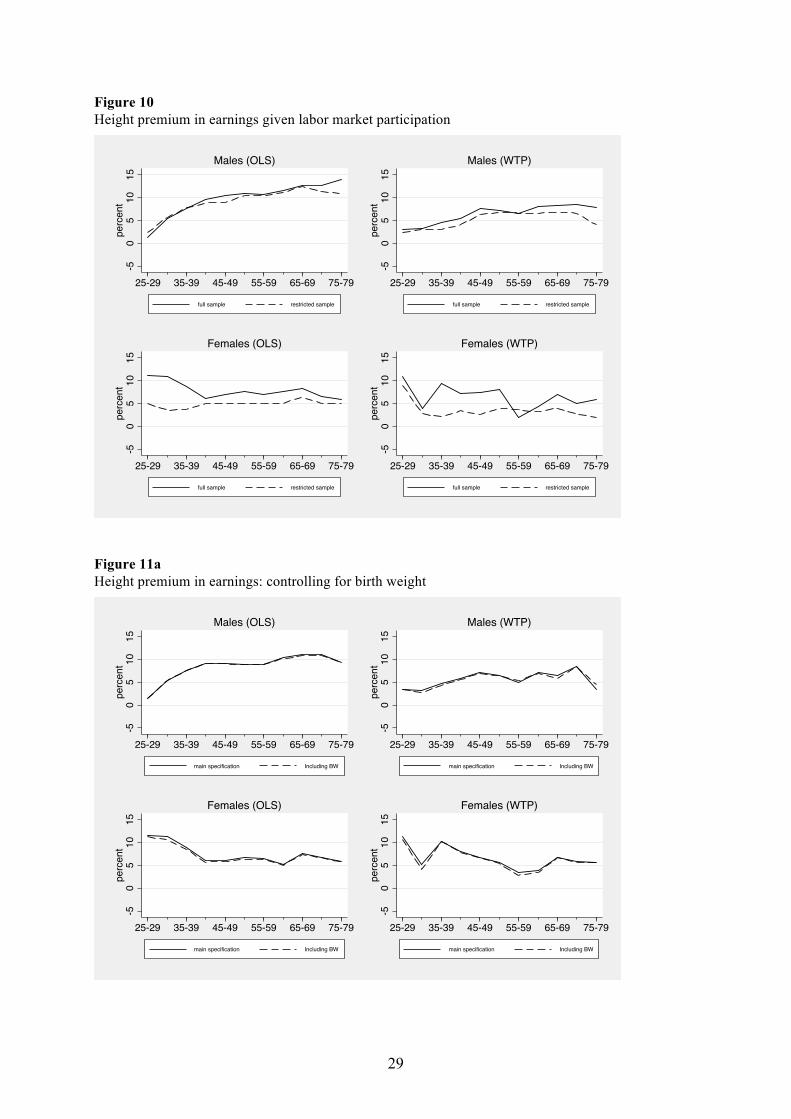
the restricted samples are shown in Figure 10.22 Imposing the earnings restriction described

above leaves the estimates for the male sample almost unchanged. In contrast, the same

restriction decreases the height coefficients for the female sample for most of the considered

age waves. This implies that parts of the unrestricted female height premium could be

attributed to a positive association between height and labor market participation. In this

setting, the return to tallness for women is shown to be relatively constant throughout the life

cycle amounting to about 5 percent in the OLS setting and 3-4 percent in the WTP setting.

21 The PBA is a measure commonly used in Swedish law to define benefits and public insurance terms. It strictly follows the consumer price index over time and amounted to SEK 44,400 (or about USD 6,000) in 2010. Two PBAs is a very low income in Sweden. A study of seven major labor market negotiation sectors in 2004 (there are no legislated minimum wages in Sweden, but wages are set by negotiations between unions and employer organizations) showed that the very lowest monthly full-time salary was 12,790 SEK (Skedinger, 2006). On an annual basis, two PBAs were equivalent to 51 percent of this. Hence, the income restriction excludes individuals whose total earnings do not exceed the revenue from working half-time at the lowest wage. 22 Height coefficients with standard errors clustered by twin pair are also presented in Table A.7 in Appendix.

17

Birth Weight and Height as Proxies for In Utero Environmental Conditions

The relationship between height and earnings could be a function of in utero and

infancy conditions, which in turn should be mirrored by birth weight and birth height.23 If the

association between height and earnings could be traced back to such environmental

conditions, including birth indicators in the model would lower the estimates of the height

premium.24

Introducing birth weight or birth height into our model leaves the estimated height

premium coefficients nearly identical to the main specification, which can be seen in Figure

11a and 11b (see also table A.8).25 Hence, we conclude that within twin-pair differences of in

utero and infancy conditions, do not explain differences in the height premium.

Educational Attainment as a Mediating Variable

Several studies have shown that height and cognitive ability is positively correlated over

the life span, also among twins (Beauchamp et al., 2011; Case and Paxson, 2008a; Case and

Paxson, 2008b; Keller et al., 2013; Richards et al., 2002; Tanner, 1979). If cognitive ability,

and thereby also height, also is related to length of education it seems reasonable to believe

that educational attainment could function as a mediating variable for the height-earnings

relationship over the life cycle.26

Figure 12 (see also table A.9) illustrates the height coefficients for the main

specification and specifications in which we include years of schooling.27 Variations in

educational attainment between individuals as captured in the main unconditional OLS model

decreases the height premium estimates by approximately 40 percent for the male sample and

more than 50 percent for the female sample. However, the conditional WTP height premiums

remain almost unchanged for both genders when introducing years of schooling. Hence, intra-

familial variation in education does not seem to affect the associated estimated height

23 It has been shown that birth weight is correlated with both adult height and labor market outcomes such as earnings (e.g., Black et al., 2007). For the (pooled) sample used in this study, the correlation between adult height and birth weight is 0.19 and statistically significant. 24 The average difference in birth weight for DZ twins is approximately 360 grams for males and about 340 grams for females. The average difference in birth weight for MZ twins is close to 300 grams for both men and women. Close to 91 percent of sample have a birth weight difference of at least 50 grams. 25 Height and birth weight coefficients with standard errors clustered by twin pair are also presented in Table A.8 in Appendix. 26 The average difference in years of schooling for DZ twins is 1.9 years for males and 1.6 years for females. The average difference in schooling for MZ twins is 1.3 years for both men and women. 53 percent of the full sample have nonzero within twin-pair differences in years of schooling. 27 Height and years-of-schooling coefficients with standard errors clustered by twin pair are also presented in Table A.9 in Appendix.

18

premium at all. Moreover, and as shown by Figure 13, introducing years of schooling into the

model specification for men yields almost identical OLS and WTP height coefficients.

Overall, this suggests that the mechanisms behind the height premium that can be traced back

to family background and genetics (that are differenced out in the WTP specifications) are

mediated through variations in educational attainment between families. For women, the

results of including schooling are less transparent (the WTP estimates are mostly larger for

younger ages, but close to the OLS estimates for older ages).

5 Concluding Discussion

It is widely known that tall people earn more than people of limited stature. This study

primarily explores how the height premium in earnings develops with age, whether this

pattern has changed over time, and to which extent the crude height premium can be traced

back to early life conditions (family background) and genetic predispositions. Our estimations

show that the profiles of the returns to tallness over the life cycle vary between men and

women. For men, the height premium increases with age, a pattern that qualitatively remains,

tough less pronounced, when differencing between twins. Moreover, the height premium at a

given age tends to fall across cohorts. A positive development of the height premium for men

is not consistent with discriminatory models in which employers erroneously accredit

capabilities to (young) people according to their height and such misperceptions eventually

unfold. Increasing height premiums with age are consistent with a scenario in which

productivity-related individual characteristics such as cognition and non-cognitive skills (and

skill development) are associated with height, and such characteristics promote career

building and earnings growth. But it would also be consistent with a situation in which taller

individuals throughout their careers are, regardless of their skills, positively discriminated

when it comes to promotions to higher, better paid occupations or positions. The data material

at hand does not allow us to discriminate between these hypotheses. Further, the height

premium in earnings is not limited to active labor market participation but spills over on

retirement via pension reimbursements.

The height premium in earnings tends to decrease with age for women, but the

estimated pattern is more volatile. However, taking labor market participation into account,

the estimated height premiums are rather constant with age. Again, the data at hand does not

allow us to discern whether this may be a function of age independent height related

19

discrimination or a result of height being associated with productivity related traits. Generally,

it appears as that tallness matter more for the earnings of men than of women.

For both males and females, the association between height and earnings has become

somewhat weaker over time. The childhood and youth of the studied birth cohorts, ranging

from 1900-1958, cover a period in which Sweden was transformed into a more modern

welfare state. It seems plausible that this also meant that the total variation in height within

the population became relatively more attributable to genetic and less to environmental

factors. If there is an association between environmentally induced height and cognitive

capability, which is stronger than the corresponding association between genetically induced

height and cognition, it follows that the association between height and earnings should be

expected to decrease when environmentally insults becomes more limited in a developing

society. However, a decrease in the height premium over time would also be consistent with

structural changes of the labor market in which, for example, height-based discrimination is

decreasing.

Within twin-pair fixed effects estimates are on average 40 percent lower than the OLS

estimates for men, suggesting that early life environmental conditions and genetic

endowments explain a significant part of the unconditional returns to tallness throughout most

of an individual’s adult life. Including education as an explanatory variable has no effect on

the within twin pair estimates, whereas it induces a similar reduction (about 40 percent) of the

estimated OLS height premium, implying that the OLS and WTP height premium patterns

now tend to coincide. Hence, it seems as if schooling may mediate the association between

height and earnings among unrelated male individuals, but not twins.

20

References

Almond, D, Currie, J. (2011), “Human Capital Development before Age Five,” Handbook of

Labor Economics, David Card and Orley Ashenfelter (eds.).

Barker, D. (2007). "The origins of the developmental origins theory." Journal of Internal

Medicine, 261: 412-417.

Beauchamp, J.P., Cesarini, D., Johannesson, M., Lindqvist, E., Apicella, C. (2011). “On the

sources of the height-intelligence correlation: New insights from a bivariate ACE model with

assortative mating.” Behavior Genetics, 41 (2), pp. 242-252.

Black, S. E., Devereux, P. J., and Salvanes, K. G. (2007). “From the cradle to the labor

market? The effect of birth weight on adult outcomes.” Quarterly Journal of Economics,

122(1): 409-439

Böckerman, P., & Vainiomäki, J. (2013). ”Stature and life-time labor market outcomes:

Accounting for unobserved differences.” Labour Economics, 24, 86-96.

Böhlmark, A., and M. Lindquist (2006). “Life- Cycle Variations in the Association Between

Current and Lifetime Income: Replication and Extension for Sweden.” Journal of Labor

Economics, 24(4): 879–896.

Bound, John, Solon, Gary, 1999. Double trouble: on the value of twins-based estimation of

the return to schooling. Econ. Educ. Rev. 18 (2), 169–182.

Card, D. (1999). “The Return to Education.” In Handbook of Labor Economics, eds. O.

Ashenfelter and D. Card, 1801–1863. Amsterdam: Elsevier.

Case, A., and C. Paxson (2008). “Stature and status: Height, ability, and labor market

outcomes.” Journal of Political Economy, 116(3): 499-532.

Case, A., C. Paxson, and M. Islam (2009). “Making sense of the labor market height

premium: Evidence from the British household panel survey.” Economic Letters, 102(3): 174-

176.

Dahl, A. K., L. B. Hassing, E. I. Fransson, and N. L. Pedersen, (2010). “Agreement between

self-reported and measured height, weight and body mass index in old age—a longitudinal

study with 20 years of follow-up.” Age and Ageing 39(4): 445-451.

21

Elo, I. T., and S. H.Preston, (1992). “Effects of early-life conditions on adult mortality: a

review.” Population index, 58(2): 186-212.

Gowin, E. B. (1915). The executive and his control of men. New York: Macmillan.

Griliches, Z. (1977). “Estimating the returns to schooling: Some econometric problems.”

Econometrica: Journal of the Econometric Society: 1-22.

Griliches, Z. (1979). “Sibling models and data in economics: Beginnings of a survey.” The

Journal of Political Economy: 37-64.

Hamermesh, D. S., and J. E. Biddle (1994). “Beauty and the labor market.” The American

Economic Review, 84(5): 1174-1194.

Jacobs, J., and V. Tassenaar (2004). “Height, income, and nutrition in the Netherlands: the

second half of the 19th century.” Economics and Human Biology, 2(2): 181-195.

Judge, T. A., and D. M. Cable (2004). “The Effect of Physical Height on Workplace Success

and Income: Preliminary Test of a Theoretical Model.” Journal of Applied Psychology, 89(3):

428-441.

Keller, M.C., Garver-Apgar, C.E., Wright, M.J., Martin, N.G., Corley, R.P., Stallings, M.C.,

Hewitt, J.K., Zietsch, B.P. (2013). “The Genetic Correlation between Height and IQ: Shared

Genes or Assortative Mating?” PLoS Genetics, 9(4).

Komlos, J. (1990). “Height and social status in eighteenth-century Germany.”

Interdisciplinary History, 20(4): 607-621.

Lichtenstein, P., Floderus, B., Svartengren, M., Svedberg, P., & Pedersen, N. L. (2002). ”The

Swedish Twin Registry: a unique resource for clinical, epidemiological and genetic studies.”

Journal of internal medicine, 252(3): 184-205.

Lundborg P. (2013),The health returns to education –what can we learn from twins? Journal

of Population Economics. 26 (2): 673-701.

Lundborg, P., P. Nystedt, and D. O. Rooth (2014). “Height and earnings: The role of

cognitive and noncognitive skills.” Journal of Human Resources, 49(1): 141-166.

Neumark, D. (1999). ”Biases in twin estimates of the return to schooling.” Economics of

Education Review, 18(2), 143-148.

22

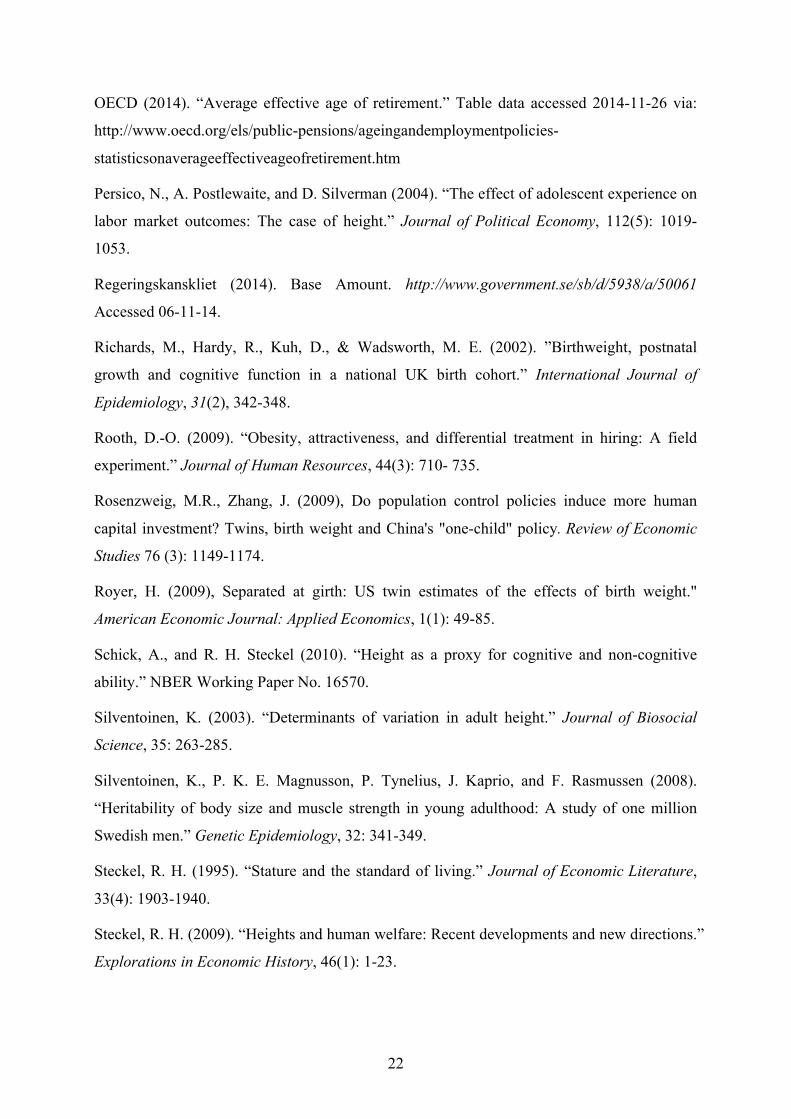
OECD (2014). “Average effective age of retirement.” Table data accessed 2014-11-26 via:

http://www.oecd.org/els/public-pensions/ageingandemploymentpolicies-

statisticsonaverageeffectiveageofretirement.htm

Persico, N., A. Postlewaite, and D. Silverman (2004). “The effect of adolescent experience on

labor market outcomes: The case of height.” Journal of Political Economy, 112(5): 1019-

1053.

Regeringskanskliet (2014). Base Amount. http://www.government.se/sb/d/5938/a/50061

Accessed 06-11-14.

Richards, M., Hardy, R., Kuh, D., & Wadsworth, M. E. (2002). ”Birthweight, postnatal

growth and cognitive function in a national UK birth cohort.” International Journal of

Epidemiology, 31(2), 342-348.

Rooth, D.-O. (2009). “Obesity, attractiveness, and differential treatment in hiring: A field

experiment.” Journal of Human Resources, 44(3): 710- 735.

Rosenzweig, M.R., Zhang, J. (2009), Do population control policies induce more human

capital investment? Twins, birth weight and China's "one-child" policy. Review of Economic

Studies 76 (3): 1149-1174.

Royer, H. (2009), Separated at girth: US twin estimates of the effects of birth weight."

American Economic Journal: Applied Economics, 1(1): 49-85.

Schick, A., and R. H. Steckel (2010). “Height as a proxy for cognitive and non-cognitive

ability.” NBER Working Paper No. 16570.

Silventoinen, K. (2003). “Determinants of variation in adult height.” Journal of Biosocial

Science, 35: 263-285.

Silventoinen, K., P. K. E. Magnusson, P. Tynelius, J. Kaprio, and F. Rasmussen (2008).

“Heritability of body size and muscle strength in young adulthood: A study of one million

Swedish men.” Genetic Epidemiology, 32: 341-349.

Steckel, R. H. (1995). “Stature and the standard of living.” Journal of Economic Literature,

33(4): 1903-1940.

Steckel, R. H. (2009). “Heights and human welfare: Recent developments and new directions.”

Explorations in Economic History, 46(1): 1-23.

23

Stunkard, A. J., T.T. Foch and Z. Hrubec (1986). "A twin study of human obesity." Jama

256(1): 51-54.

Sundet, J. M., Tambs, K., Harris, J. R., Magnus, P., & Torjussen, T. M. (2005). ”Resolving

the genetic and environmental sources of the correlation between height and intelligence: A

study of nearly 2600 Norwegian male twin pairs.” Twin Research and Human Genetics,

8(04), 307-311.

Tanner James M. A Concise History of Growth Studies from Buffon to Boas (1979). Chapter

17. In: Falkner Frank, Tanner JM., editors. Human Growth, Volume 3, Neurobiology and

Nutrition. New York: 1979. pp. 515–593.

Thomas, D., and J. Strauss (1997). Health and wages: Evidence on men and women in urban

brazil. Journal of Econometrics, 77(1): 159-185.

Wildman, J. (2003). Modelling health, income and income inequality: the impact of income

inequality on health and health inequality. Journal of Health Economics, 22(4): 521-538.

24

Figures Figure 1 Distribution of within twin-pair height differences

Figure 2 Average annual earnings by age

0.1

.2.3

.4De

nsity

0 5 10 15 20 25 30 35centimeters

DZ MZ

Males

0.1

.2.3

.4De

nsity

0 5 10 15 20 25 30 35centimeters

DZ MZ

Females

010

020

030

0SE

K 10

00

25-29 35-39 45-49 55-59 65-69 75-79age

DZ males MZ malesDZ females MZ females

25

Figure 3 Average annual earnings (SEK 1000) by height for different age groups, males

Figure 4 Average annual earnings (SEK 1000) by height for different age groups, females

020

040

060

0

150 160 170 180 190 200height (cm)

25-29

020

040

060

0150 160 170 180 190 200

height (cm)

30-34

020

040

060

0

150 160 170 180 190 200height (cm)

35-39

020

040

060

0

150 160 170 180 190 200height (cm)

40-44

020

040

060

0

150 160 170 180 190 200height (cm)

45-49

020

040

060

0

150 160 170 180 190 200height (cm)

50-54

020

040

060

0150 160 170 180 190 200

height (cm)

55-59

020

040

060

0

150 160 170 180 190 200height (cm)

60-64

020

040

060

0

150 160 170 180 190 200height (cm)

65-69

020

040

060

0

150 160 170 180 190 200height (cm)

70-74

020

040

060

0

150 160 170 180 190 200height (cm)

75-79

010

020

030

0

150 160 170 180 190 200height (cm)

25-29

010

020

030

0

150 160 170 180 190 200height (cm)

30-34

010

020

030

0

150 160 170 180 190 200height (cm)

35-39

010

020

030

0

150 160 170 180 190 200height (cm)

40-44

010

020

030

0

150 160 170 180 190 200height (cm)

45-49

010

020

030

0

150 160 170 180 190 200height (cm)

50-54

010

020

030

0

150 160 170 180 190 200height (cm)

55-59

010

020

030

0

150 160 170 180 190 200height (cm)

60-64

010

020

030

0

150 160 170 180 190 200height (cm)

65-69

010

020

030

0

150 160 170 180 190 200height (cm)

70-74

010

020

030

0

150 160 170 180 190 200height (cm)

75-79

26

Figure 5 Average annual earnings at age 30-39 by height

Figure 6 The unconditional and conditional height premiums in earning

5010

015

020

025

030

0SE

K 10

00

150 160 170 180 190 200height (cm)

5010

015

020

025

030

0SE

K 10

00150 160 170 180 190

height (cm)

-50

510

15pe

rcen

t

25-29 35-39 45-49 55-59 65-69 75-79age

Males (OLS)

-50

510

15pe

rcen

t

25-29 35-39 45-49 55-59 65-69 75-79age

Males (WTP)

-50

510

15pe

rcen

t

25-29 35-39 45-49 55-59 65-69 75-79age

Females (OLS)

-50

510

15pe

rcen

t

25-29 35-39 45-49 55-59 65-69 75-79age

Females (WTP)

27

Figure 7 The height premium in earnings: gender differences

05

1015

perce

nt

25-29 35-39 45-49 55-59 65-69 75-79age

males females

OLS

05

1015

perce

nt25-29 35-39 45-49 55-59 65-69 75-79

age

males females

WTP

28

Figure 8 The height premium in earnings: birth cohorts born 1900-1919, 1920-1939, 1940-1958

Figure 9 The height premium in earnings: improtance of early life environmental conditions and genes

-10

-50

510

1520

25-29 35-39 45-49 55-59 65-69 75-79

1900-1919 1920-1939

1940-1958

Males (OLS)

-10

-50

510

1520

25-29 35-39 45-49 55-59 65-69 75-79

1900-1919 1920-1939

1940-1958

Males (WTP)

-10

-50

510

1520

25-29 35-39 45-49 55-59 65-69 75-79

1900-1919 1920-1939

1940-1958

Females (OLS)

-10

-50

510

1520

25-29 35-39 45-49 55-59 65-69 75-79

1900-1919 1920-1939

1940-1958

Females (WTP)

-50

510

15pe

rcen

t

25-29 35-39 45-49 55-59 65-69 75-79

OLS: pooled sample WTP: DZ twinsWTP: MZ twins

Males

-50

510

15pe

rcen

t

25-29 35-39 45-49 55-59 65-69 75-79

OLS: pooled sample WTP: DZ twinsWTP: MZ twins

Females

29

Figure 10 Height premium in earnings given labor market participation

Figure 11a Height premium in earnings: controlling for birth weight

-50

510

15pe

rcen

t

25-29 35-39 45-49 55-59 65-69 75-79

full sample restricted sample

Males (OLS)

-50

510

15pe

rcen

t

25-29 35-39 45-49 55-59 65-69 75-79

full sample restricted sample

Males (WTP)

-50

510

15pe

rcen

t

25-29 35-39 45-49 55-59 65-69 75-79

full sample restricted sample

Females (OLS)

-50

510

15pe

rcen

t

25-29 35-39 45-49 55-59 65-69 75-79

full sample restricted sample

Females (WTP)

-50

510

15pe

rcen

t

25-29 35-39 45-49 55-59 65-69 75-79

main specification Including BW

Males (OLS)

-50

510

15pe

rcen

t

25-29 35-39 45-49 55-59 65-69 75-79

main specification Including BW

Males (WTP)

-50

510

15pe

rcen

t

25-29 35-39 45-49 55-59 65-69 75-79

main specification Including BW

Females (OLS)

-50

510

15pe

rcen

t

25-29 35-39 45-49 55-59 65-69 75-79

main specification Including BW

Females (WTP)

30

Figure 11b Height premium in earnings: controlling for birth height

Figure 12 Height premium in earnings: controlling for educational attainment

-50

510

15pe

rcen

t

25-29 35-39 45-49 55-59 65-69 75-79

main specification Including BL

Males (OLS)

-50

510

15pe

rcen

t

25-29 35-39 45-49 55-59 65-69 75-79

main specification Including BL

Males (WTP)

-50

510

15pe

rcen

t

25-29 35-39 45-49 55-59 65-69 75-79

main specification Including BL

Females (OLS)

-50

510

15pe

rcen

t

25-29 35-39 45-49 55-59 65-69 75-79

main specification Including BL

Females (WTP)

-50

510

15pe

rcen

t

25-29 35-39 45-49 55-59 65-69 75-79

main specification Including years of schooling

Males (OLS)

-50

510

15pe

rcen

t

25-29 35-39 45-49 55-59 65-69 75-79

main specification Including years of schooling

Males (WTP)

-50

510

15pe

rcen

t

25-29 35-39 45-49 55-59 65-69 75-79

main specification Including years of schooling

Females (OLS)

-50

510

15pe

rcen

t

25-29 35-39 45-49 55-59 65-69 75-79

main specification Including years of schooling

Females (WTP)

31

Figure 13 Height premium in earnings and educational attainment: OLS versus WTP estimates

-50

510

15percent

25-29 35-39 45-49 55-59 65-69 75-79

OLS WTP

Males

-50

510

15percent

25-29 35-39 45-49 55-59 65-69 75-79

OLS WTP

Females

32

Tables Table 1 Descriptive statistics

males females

DZ MZ DZ MZ

Height

Height in cm 176.4 176.1 163.6 163.5 (6.8) (6.7) (5.9) (5.8) Within twin pair height difference in cm 5.0 2.3 4.6 2.1

(4.1) (2.5) (3.7) (2.4) Number of zero differences in height 956 1,592 1,224 2,132

Educational Attainment

Years of Schooling 9.6 9.8 9.2 9.7 (3.3) (3.4) (3.2) (3.2) Within twin pair difference in schooling 1.909 1.360 1.607 1.300 (2.286) (1.940) (2.021) (1.828)

Observations 12,372 7,610 14,462 9,036

Annual Earnings

Average annual earnings at age 30-39 237,015 241,796 123,165 128,096

(87,524) (87,257) (69,865) (70,609)

Observations 7,502 4,830 7,574 5,322

Birth weight

Birth weight in grams 2,756 2,661 2,644 2,494 (508) (497) (497) (492)

Observations 6,616 4,190 7,006 4,900

Birth height

Birth height in cm 48.27 47.53 47.56 46.77

(2.739) (2.800) (2.769) (2.828)

Observations 6566 4174 6966 4876

Notes: Mean coefficients with standard deviations in parentheses presented by zygosity and gender. Annual earnings (SEK) in 2010 price levels, winsorized at the 1st and the 99th percentiles. Data on birth weight is restricted to a subsample born 1925-1958.

33

Table 2 Descriptive statistics: Cohorts born 1900-1919, 1920-1939, 1940-1958

Variable males females

DZ MZ DZ MZ Cohort born 1900-1919

Height

Height in cm 173.3 173.1 161.8 161.3 (6.3) (6.1) (5.9) (5.7) Within twin pair height difference in cm 5.2 2.5 4.8 2.6 (4.3) (2.4) (3.9) (3.0) Number of zero difference in height 210 264 286 386

Educational Attainment Years of Schooling 7.4 7.5 7.0 7.2 (2.5) (2.5) (2.1) (2.2)

Observations 2,624 1,542 3,414 1,794 Cohort born 1920-1939

Height Height in cm 175.6 175.1 163.1 163.1 (6.3) (6.4) (5.6) (5.6) Within twin pair height difference in cm 4.9 2.4 4.6 2.0 (3.9) (2.7) (3.6) (2.1) Number of zero difference in height 292 498 372 666 Educational Attainment Years of Schooling 9.0 9.2 8.5 9.0 (3.4) (3.4) (3.0) (3.2)

Observations 4,084 2,344 4,850 2,886 Cohort born 1940-1958

Height Height in cm 178.8 178.4 165.4 164.9 (6.4) (6.3) (5.7) (5.5)

Within twin pair height difference in cm 5.0 2.1 4.5 1.9

(4.0) (2.3) (3.7) (1.9) Number of zero difference in height 436 778 518 1,050

Educational Attainment Years of Schooling 11.1 11.5 11.3 11.5 (2.8) (2.8) (2.6) (2.6)

Observations 5,368 3,514 5,750 4,128 Notes: Mean coefficients with standard deviations in parentheses presented by zygosity and gender. Annual earnings (SEK) in 2010 price levels, winsorized at the 1st and the 99th percentiles.

34

Table 3 The height premium in earnings at age 30-39     (1) (2) (3) (4) DZ MZ DZ MZ Males Height 0.074*** 0.063*** 0.042*** 0.029 (0.008) (0.011) (0.013) (0.023)

Observations 7,502 4,830 7,502 4,830 Females            Height 0.102*** 0.088*** 0.078*** 0.070 (0.021) (0.025) (0.034) (0.078)

Observations 7,574 5,322 7,574 5,322 Notes: Columns 1-2 present OLS regression coefficients, of which both model specifications include birth-year fixed effects. Columns 3-4 present within twin pair regression coefficients. Columns 1 and 3 report coefficients for the dizygotic (DZ) twin sample and columns 2 and 4 report coefficients for the monozygotic (MZ) twin sample. Standard errors in parentheses, clustered by twin pair in all specifications. Significance level: *** p<0.01, ** p<0.05, * p<0.1. Dependent variable is logarithm of average annual earnings at age 30-39, winsorized at the 1st and 99th percentiles. Height coefficients are presented in terms of decimeters.

Table 4 Number of observations in original sample and sample in which annual earnings is at least SEK 84,800

Sample males   females

Original > SEK 84,800 Difference (%) Original > SEK 84,800 Difference (%)

Age 25-29 9,220 6,978 24% 8,956 5,050 44% 30-34 10,870 10,144 7% 10,686 5,706 47% 35-39 12,226 11,502 6% 12,658 7,780 39% 40-44 13,600 12,776 6% 14,452 10,514 27% 45-49 15,102 14,062 7% 16,120 12,478 23% 50-54 15,926 14,710 8% 17,004 13,246 22% 55-59 14,646 13,296 9% 15,662 11,776 25% 60-64 12,542 11,150 11% 14,718 9,422 36% 65-69 9,806 8,326 15% 12,860 6,146 52% 70-74 7,184 5,434 24% 10,136 4,116 59% 75-79 4,594 3,132 32% 7,624 2,868 62% Note: The table reports the number of observations in the original sample used in the main analysis and the number of observations in the sample of twin pairs in which both have average annual earnings of at least SEK 84,800 (in 2010 prices). The relative difference (%) in sample sizes relative to original sample size is also presented.

35

Appendix Measurement Error in Self-Reported Height Among Twins

Measurement errors in explanatory variables may induce an attenuation bias in the

estimation of such variables. In the presence of such errors, the bias of the OLS estimator of

an explanatory variable is given by σv/σS, where σv is the variance of the actual misreports

and σS is the variance in the reported value of the explanatory variable (see, for example,

Neumark, 1999; Bound and Solon, 1999). In the case of classical measurement errors, this

bias is inflated when differencing among, for example, twins, and the bias now becomes

σv/[σS(1-ρS)], where ρS is the correlation between the reported explanatory variable within

twin pairs. Hence, the attenuation bias increases in the correlation (ρS), as long as this

correlation is positive. According to our previous argument, we expect the measurement

errors to be rather mild in the present study, and also non-classical as they ought to be

correlated within twin pairs implying that the actual error of the difference in height between

twins will be less pronounced than any misreports per se. From this perspective it is

reassuring that our WTP height premium estimate (4.2 percent per decimeter height) among

male DZ twins aged 30-39 coincides with the corresponding estimate obtained via

differencing of administratively recorded height data among a large-scale representative

sample of brothers by Lundborg et al. (2014).

If measurement errors were not correlated within twin pairs we would expect the

variance of the difference between twins to grow substantially with age since the

measurement errors per se are likely to grow with age. As indicated by Table 2, however, it

seems that this is not the case. For DZ male twin pairs, the average difference in height and

the corresponding variance hereof (in parenthesis) amounts to 5.0 (4.0), 4.9 (3.9) and 5.2 (4.3)

for the cohorts born 1940-1958, 1920-1939 and 1900-1919, respectively. The corresponding

figures for male MZ twin pairs are 2.1 (2.3), 2.4 (2.7) and 2.5 (2.4). For women the DZ

figures are 4.5 (3.7), 4.6 (3.6) and 4.8 (3.9) and for MZ twins they are 1.9 (1.9), 2.0 (2.1) and

2.6 (3.0). Apart from the oldest female cohort MZ twin sample, the difference in height

between twins and the variance hereof are remarkable stable across cohorts.

Unfortunately we do not have data on the measurement errors in height in our sample

making direct analysis of actual measurement errors impossible. However, an indirect

assessment of the importance of measurement errors could be obtained by comparing MZ and

DZ twins from this respect. The magnitude in WTP parameter estimations of the bias from

measurement errors (assumed to be randomly distributed among the twins) hinges critically

36

on the correlation of the reported heights of the twins within a pair (see, for example,

Griliches, 1977; Griliches, 1979; Neumark, 1999; Bound and Solon 1999). In our sample the

within twin pair correlation of height amounts to (0.55, 0.87) and (0.50, 0.85) for (DZ, MZ)

men and women respectively. Combined with the variance of the reported height in the

respective sample (46, 45; 35,34: see the reported standard errors in Table 1) this implies that

the downward bias should be about four times greater in the MZ sample compared to the DZ

sample. Now, the absolute values of these biases are dependent on the variance of the

measurement error, which we do not have. Fortunately, this has been estimated to amount to

4.4 centimeters in a subsample of the data used here for people aged 40-88 (mean age 63.9)

by Dahl et al. (2010). Using this value (which is probably an overestimate, since the

measurement error increases with age) in our computations, the measurement error bias

would amount to about 10 percent in the OLS, 20-25 percent in the WTP DZ estimations and

75-90 percent in the WTP MZ estimations. Hence, in the presence of randomly distributed

classical measurement errors, we would expect the DZ estimates to be much closer to the

OLS than to the MZ estimates, which in turn should be close to zero. From this respect, the

fact that the DZ estimates is much closer to the MZ ones implies not only that, within twin

pairs, the height variation has similar effect on earnings regardless of whether it is genetically

or environmentally induced, but also that the estimates are rather unaffected by measurement

errors. Though admittedly circumstantial, the arguments above suggest that measurement

errors are not heavily influencing the results.

38

Table A.1 The height premium in earnings over the life cycle (1) (2) (3) (4) (5) (6) (7) (8) (9) (10) (11)

Age 25-29 30-34 35-39 40-44 45-49 50-54 55-59 60-64 65-69 70-74 75-79 Males (A) Height 0.014 0.055*** 0.076*** 0.095*** 0.105*** 0.109*** 0.107*** 0.115*** 0.126*** 0.127*** 0.139*** (0.008) (0.007) (0.007) (0.007) (0.008) (0.008) (0.009) (0.009) (0.009) (0.010) (0.0133) Observations 9,220 10,870 12,226 13,600 15,102 15,926 14,646 12,542 9,806 7,184 4,594 (B) Height 0.031** 0.033*** 0.045*** 0.055*** 0.076*** 0.072*** 0.066*** 0.079*** 0.082*** 0.084*** 0.079*** (0.015) (0.012) (0.013) (0.013) (0.014) (0.015) (0.015) (0.016) (0.014) (0.017) (0.023) Observations 9,220 10,870 12,226 13,600 15,102 15,926 14,646 12,542 9,806 7,184 4,594 Females    (C) Height 0.112*** 0.108*** 0.087*** 0.062*** 0.070*** 0.077*** 0.070*** 0.076*** 0.083*** 0.066*** 0.059*** (0.021) (0.019) (0.016) (0.013) (0.011) (0.011) (0.013) (0.013) (0.008) (0.009) (0.009) Observations 8,956 10,686 12,658 14,452 16,120 17,004 15,662 14,718 12,860 10,136 7,624    (D) Height 0.109*** 0.040 0.095*** 0.072*** 0.074*** 0.080*** 0.018 0.043* 0.069*** 0.051*** 0.058*** (0.040) (0.038) (0.032) (0.027) (0.024) (0.022) (0.025) (0.026) (0.015) (0.015) (0.016) Observations 8,956 10,686 12,658 14,452 16,120 17,004 15,662 14,718 12,860 10,136 7,624 Notes: Columns 1-11 present the height coefficients for earnings at the 11 age waves, 25-79. Row (A) and (C) reports the OLS regression coefficients, of which all model specifications include birth year fixed effects. Row (B) and (D) report within twin pair regression coefficients. All model specifications are for the pooled sample (DZ and MZ twins). Standard errors parentheses, clustered by twin pair in all model specifications. Significance level: *** p<0.01, ** p<0.05, * p<0.1. Dependent variable is logarithm of average annual earnings, winsorized at the 1st and 99th percentiles. Height coefficients are presented in terms of decimeters.

39

Table A.2 The unconditional height premium in earnings: birth cohorts born 1900-1919, 1920-1939, 1940-1958, males (1) (2) (3) (4) (5) (6) (7) (8) (9) (10) (11)

Age 25-29 30-34 35-39 40-44 45-49 50-54 55-59 60-64 65-69 70-74 75-79 Cohort born 1900-1919 (A) Height - - - - - 0.158*** 0.141*** 0.129*** 0.136*** 0.137*** 0.148*** - - - - - (0.033) (0.025) (0.021) (0.018) (0.018) (0.021) Observations - - - - - 1,666 2,834 3,456 3,576 2,910 2,090

Cohort born 1920-1939    (B) Height - 0.080*** 0.096*** 0.123*** 0.137*** 0.127*** 0.125*** 0.125*** 0.126*** 0.121*** 0.112*** - (0.019) (0.015) (0.012) (0.012) (0.012) (0.012) (0.012) (0.011) (0.012) (0.016) Observations - 2,044 3,498 4,968 6,328 6,190 5,912 5,584 5,064 3,880 2,100

Cohort born 1940-1958    (C) Height 0.014 0.049*** 0.069*** 0.079*** 0.081*** 0.086*** 0.073*** 0.086*** 0.098*** - - (0.008) (0.008) (0.008) (0.009) (0.010) (0.012) (0.014) (0.018) (0.027) - - Observations 8,874 8,826 8,728 8,632 8,498 8,070 5,900 3,502 1,084 - -

Notes: Columns 1-11 present the OLS height coefficients for earnings at the 11 age waves, 25-79, of which all model specifications include birth year fixed effects. All model specifications are for the pooled sample (DZ and MZ twins). Standard errors in parentheses, clustered by twin pair in all model specifications. Significance level: *** p<0.01, ** p<0.05, * p<0.1. Dependent variable is logarithm of average annual earnings, winsorized at the 1st and 99th percentiles. Height coefficients are presented in terms of decimeters.

40

Table A.3 The conditional height premium in earnings: birth cohorts born 1900-1919, 1920-1939, 1940-1958, males (1) (2) (3) (4) (5) (6) (7) (8) (9) (10) (11)

Age 25-29 30-34 35-39 40-44 45-49 50-54 55-59 60-64 65-69 70-74 75-79 Cohort born 1900-1919 (A) Height - - - - - 0.074 0.118*** 0.095*** 0.102*** 0.077*** 0.082** - - - - - (0.052) (0.037) (0.032) (0.025) (0.027) (0.036) Observations - - - - - 1,666 2,834 3,456 3,576 2,910 2,090

Cohort born 1920-1939    (B) Height - 0.050 0.050** 0.059*** 0.091*** 0.085*** 0.092*** 0.107*** 0.081*** 0.082*** 0.071** - (0.032) (0.024) (0.021) (0.020) (0.021) (0.020) (0.022) (0.018) (0.020) (0.031) Observations - 2,044 3,498 4,968 6,328 6,190 5,912 5,584 5,064 3,880 2,100

Cohort born 1940-1958    (C) Height 0.031** 0.033*** 0.045*** 0.055*** 0.080*** 0.072*** 0.052*** 0.073*** 0.067*** - - (0.015) (0.012) (0.013) (0.013) (0.014) (0.015) (0.016) (0.018) (0.017) - - Observations 9,220 10,870 12,226 13,600 14,826 14,260 11,812 9,086 6,148 - -

Notes: Columns 1-11 present the WTP height coefficients for earnings at the 11 age waves, 25-79. All model specifications are for the pooled sample (DZ and MZ twins). Standard errors in parentheses, clustered by twin pair in all model specifications. Significance level: *** p<0.01, ** p<0.05, * p<0.1. Dependent variable is logarithm of average annual earnings, winsorized at the 1st and 99th percentiles. Height coefficients are presented in terms of decimeters.

41

Table A.4 The unconditional height premium in earnings: birth cohorts born 1900-1919, 1920-1939, 1940-1958, females (1) (2) (3) (4) (5) (6) (7) (8) (9) (10) (11)

Age 25-29 30-34 35-39 40-44 45-49 50-54 55-59 60-64 65-69 70-74 75-79 Cohort born 1900-1919 (A) Height - - - - - 0.075 0.094* 0.108*** 0.096*** 0.075*** 0.072*** - - - - - (0.058) (0.050) (0.032) (0.015) (0.014) (0.013) Observations - - - - - 1,264 2,256 3,58 4,738 4,152 3,576

Cohort born 1920-1939    (B) Height - 0.144** 0.118*** 0.079*** 0.103*** 0.103*** 0.072*** 0.075*** 0.073*** 0.063*** 0.051*** - (0.067) (0.040) (0.030) (0.022) (0.020) (0.020) (0.018) (0.011) (0.011) (0.014) Observations - 1,348 3,082 4,888 6,500 6,846 6,766 6,996 6,766 5,518 3,516

Cohort born 1940-1958    (C) Height 0.109*** 0.103*** 0.077*** 0.053*** 0.047*** 0.057*** 0.058*** 0.046** 0.076*** - - (0.021) (0.020) (0.016) (0.012) (0.012) (0.011) (0.015) (0.019) (0.024) - - Observations 8,808 9,338 9,576 9,564 9,470 8,894 6,640 4,142 1,266 - -

Notes: Columns 1-11 present the OLS height coefficients for earnings at the 11 age waves, 25-79, of which all model specifications include birth year fixed effects. All model specifications are for the pooled sample (DZ and MZ twins). Standard errors in parentheses, clustered by twin pair in all model specifications. Significance level: *** p<0.01, ** p<0.05, * p<0.1. Dependent variable is logarithm of average annual earnings, winsorized at the 1st and 99th percentiles. Height coefficients are presented in terms of decimeters.

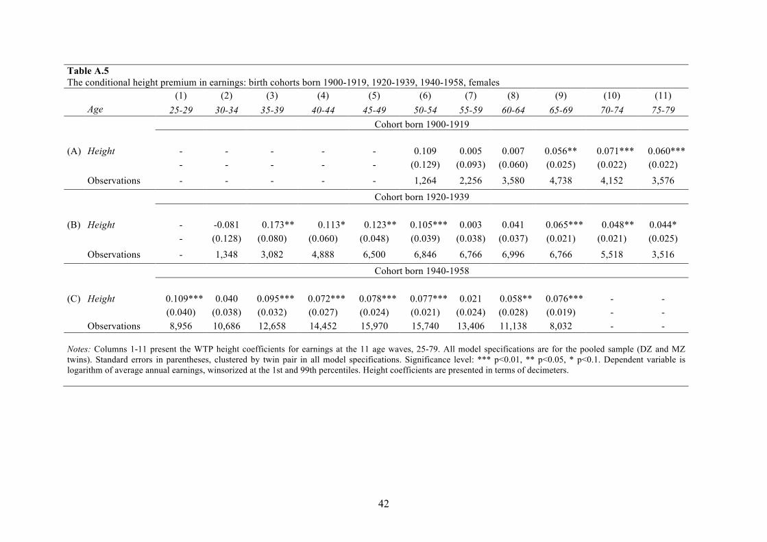
42

Table A.5 The conditional height premium in earnings: birth cohorts born 1900-1919, 1920-1939, 1940-1958, females (1) (2) (3) (4) (5) (6) (7) (8) (9) (10) (11)

Age 25-29 30-34 35-39 40-44 45-49 50-54 55-59 60-64 65-69 70-74 75-79 Cohort born 1900-1919 (A) Height - - - - - 0.109 0.005 0.007 0.056** 0.071*** 0.060*** - - - - - (0.129) (0.093) (0.060) (0.025) (0.022) (0.022) Observations - - - - - 1,264 2,256 3,580 4,738 4,152 3,576

Cohort born 1920-1939    (B) Height - -0.081 0.173** 0.113* 0.123** 0.105*** 0.003 0.041 0.065*** 0.048** 0.044* - (0.128) (0.080) (0.060) (0.048) (0.039) (0.038) (0.037) (0.021) (0.021) (0.025) Observations - 1,348 3,082 4,888 6,500 6,846 6,766 6,996 6,766 5,518 3,516

Cohort born 1940-1958    (C) Height 0.109*** 0.040 0.095*** 0.072*** 0.078*** 0.077*** 0.021 0.058** 0.076*** - - (0.040) (0.038) (0.032) (0.027) (0.024) (0.021) (0.024) (0.028) (0.019) - - Observations 8,956 10,686 12,658 14,452 15,970 15,740 13,406 11,138 8,032 - -

Notes: Columns 1-11 present the WTP height coefficients for earnings at the 11 age waves, 25-79. All model specifications are for the pooled sample (DZ and MZ twins). Standard errors in parentheses, clustered by twin pair in all model specifications. Significance level: *** p<0.01, ** p<0.05, * p<0.1. Dependent variable is logarithm of average annual earnings, winsorized at the 1st and 99th percentiles. Height coefficients are presented in terms of decimeters.

43

Table A.6 The height premium in earnings: importance of early life conditions and genes (1) (2) (3) (4) (5) (6) (7) (8) (9) (10) (11)

Age 25-29 30-34 35-39 40-44 45-49 50-54 55-59 60-64 65-69 70-74 75-79 Males DZ twins     (A) Height 0.035** 0.038*** 0.045*** 0.051*** 0.081*** 0.075*** 0.071*** 0.078*** 0.082*** 0.076*** 0.080*** (0.017) (0.014) (0.014) (0.014) (0.015) (0.016) (0.016) (0.017) (0.016) (0.019) (0.025) Observations 5,568 6,584 7,436 8,294 9,318 9,836 9,090 7,774 6,188 4,516 2,816

MZ twins     (B) Height 0.003 -0.001 0.046 0.079** 0.045 0.050 0.0357 0.089** 0.084*** 0.132*** 0.073 (0.039) (0.031) (0.028) (0.031) (0.029) (0.034) (0.031) (0.041) (0.032) (0.034) (0.052) Observations 3,652 4,286 4,790 5,306 5,784 6,090 5,556 4,768 3,618 2,668 1,778

Females DZ twins        (C) Height 0.132*** 0.034 0.100*** 0.082*** 0.079*** 0.085*** 0.026 0.041 0.073*** 0.055*** 0.055*** (0.044) (0.041) (0.035) (0.029) (0.026) (0.024) (0.028) (0.029) (0.017) (0.016) (0.018) Observations 5,156 6,178 7,424 8,512 9,610 10,208 9,500 9,106 8,138 6,440 4,862

MZ twins        (D) Height -0.034 0.079 0.061 -0.001 0.045 0.050 -0.030 0.057 0.043 0.029 0.076** (0.102) (0.097) (0.082) (0.068) (0.053) (0.052) (0.062) (0.056) (0.034) (0.034) (0.037) Observations 3,800 4,508 5,234 5,940 6,510 6,796 6,162 5,612 4,722 3,696 2,762

Notes: Columns 1-11 present the within twin-pair height coefficients for earnings at the 11 age waves, 25-79. Standard errors parentheses, clustered by twin pair in all model specifications. Significance level: *** p<0.01, ** p<0.05, * p<0.1. Dependent variable is logarithm of average annual earnings, winsorized at the 1st and 99th percentiles. Height coefficients are presented in terms of decimeters.

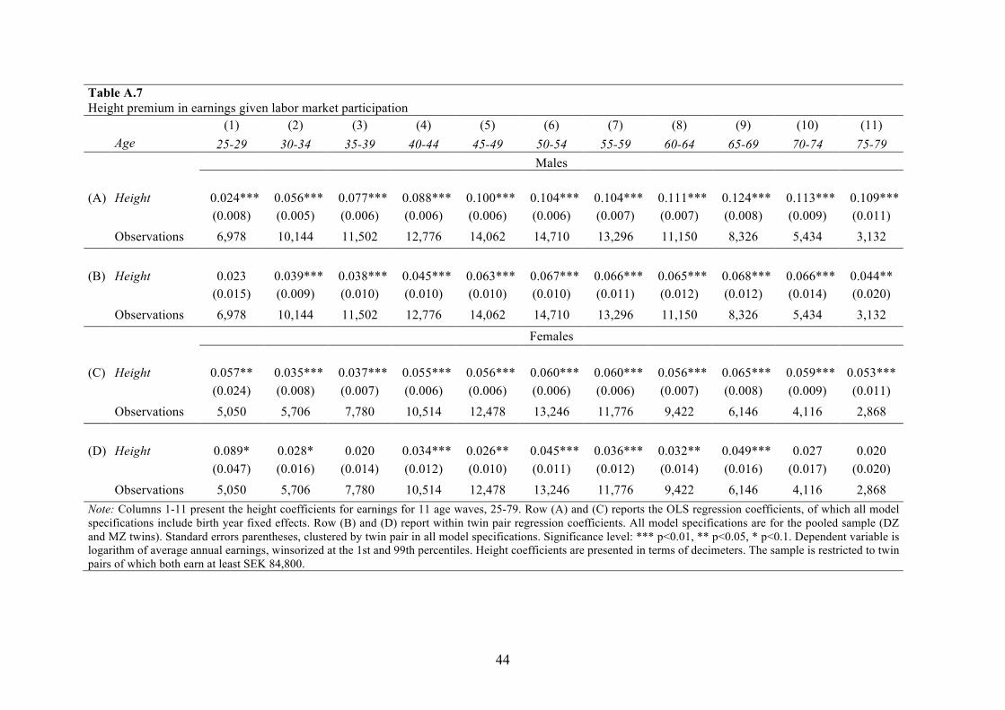
44

Table A.7 Height premium in earnings given labor market participation (1) (2) (3) (4) (5) (6) (7) (8) (9) (10) (11)

Age 25-29 30-34 35-39 40-44 45-49 50-54 55-59 60-64 65-69 70-74 75-79 Males (A) Height 0.024*** 0.056*** 0.077*** 0.088*** 0.100*** 0.104*** 0.104*** 0.111*** 0.124*** 0.113*** 0.109*** (0.008) (0.005) (0.006) (0.006) (0.006) (0.006) (0.007) (0.007) (0.008) (0.009) (0.011) Observations 6,978 10,144 11,502 12,776 14,062 14,710 13,296 11,150 8,326 5,434 3,132

(B) Height 0.023 0.039*** 0.038*** 0.045*** 0.063*** 0.067*** 0.066*** 0.065*** 0.068*** 0.066*** 0.044** (0.015) (0.009) (0.010) (0.010) (0.010) (0.010) (0.011) (0.012) (0.012) (0.014) (0.020) Observations 6,978 10,144 11,502 12,776 14,062 14,710 13,296 11,150 8,326 5,434 3,132

Females    (C) Height 0.057** 0.035*** 0.037*** 0.055*** 0.056*** 0.060*** 0.060*** 0.056*** 0.065*** 0.059*** 0.053*** (0.024) (0.008) (0.007) (0.006) (0.006) (0.006) (0.006) (0.007) (0.008) (0.009) (0.011) Observations 5,050 5,706 7,780 10,514 12,478 13,246 11,776 9,422 6,146 4,116 2,868

   (D) Height 0.089* 0.028* 0.020 0.034*** 0.026** 0.045*** 0.036*** 0.032** 0.049*** 0.027 0.020 (0.047) (0.016) (0.014) (0.012) (0.010) (0.011) (0.012) (0.014) (0.016) (0.017) (0.020) Observations 5,050 5,706 7,780 10,514 12,478 13,246 11,776 9,422 6,146 4,116 2,868 Note: Columns 1-11 present the height coefficients for earnings for 11 age waves, 25-79. Row (A) and (C) reports the OLS regression coefficients, of which all model specifications include birth year fixed effects. Row (B) and (D) report within twin pair regression coefficients. All model specifications are for the pooled sample (DZ and MZ twins). Standard errors parentheses, clustered by twin pair in all model specifications. Significance level: *** p<0.01, ** p<0.05, * p<0.1. Dependent variable is logarithm of average annual earnings, winsorized at the 1st and 99th percentiles. Height coefficients are presented in terms of decimeters. The sample is restricted to twin pairs of which both earn at least SEK 84,800.

45

Table A.8 Height premium in earnings: controlling for birth weight (1) (2) (3) (4) (5) (6) (7) (8) (9) (10) (11)

Age 25-29 30-34 35-39 40-44 45-49 50-54 55-59 60-64 65-69 70-74 75-79 Males (A) Height 0.015* 0.053*** 0.075*** 0.090*** 0.090*** 0.089*** 0.089*** 0.102*** 0.108*** 0.108*** 0.094*** (0.009) (0.007) (0.007) (0.007) (0.008) (0.009) (0.010) (0.012) (0.012) (0.015) (0.024)

Birth weight -0.00032 -0.00005 0.00031 0.00074* 0.00078* 0.00046 0.00027 0.00062 0.00160*** 0.00132* 0.00006 (0.00061) (0.00047) (0.00045) (0.00044) (0.00045) (0.00050) (0.00053) (0.00059) (0.00060) (0.00068) (0.00106)

Observations 9,112 10,748 12,082 12,874 12,680 12,154 9,816 7,270 4,556 2,564 1,118 (B) Height 0.033** 0.028** 0.043*** 0.056*** 0.069*** 0.063*** 0.053*** 0.070*** 0.059*** 0.084*** 0.045 (0.016) (0.013) (0.013) (0.013) (0.014) (0.016) (0.018) (0.022) (0.021) (0.025) (0.046) Birth weight 0.00132 0.00418** 0.00291 0.00205 0.00166 0.00056 -0.00202 0.00105 0.00441 0.00007 -0.00608 (0.00192) (0.00172) (0.00179) (0.00175) (0.00178) (0.00218) (0.00242) (0.00286) (0.00293) (0.00346) (0.00610) Observations 9,112 10,748 12,082 12,874 12,680 12,154 9,816 7,270 4,556 2,564 1,118 Females    (C) Height 0.112*** 0.106*** 0.085*** 0.057*** 0.058*** 0.063*** 0.063*** 0.051*** 0.073*** 0.066*** 0.058*** (0.022) (0.019) (0.016) (0.013) (0.011) (0.010) (0.013) (0.015) (0.012) (0.014) (0.018) Birth weight 0.00162 0.00258** 0.00148 0.00157** 0.00172*** 0.00163*** 0.00136** 0.00070 0.00123** 0.00062 0.00107 (0.00139) (0.00118) (0.00096) (0.00074) (0.00065) (0.00063) (0.00062) (0.00070) (0.00053) (0.00058) (0.00077) Observations 8,794 10,496 12,434 13,812 14,060 13,554 11,220 8,722 5,696 3,458 1,758    (D) Height 0.107*** 0.041 0.102*** 0.078*** 0.067*** 0.054*** 0.028 0.034 0.066*** 0.057** 0.057 (0.042) (0.039) (0.033) (0.029) (0.023) (0.020) (0.023) (0.029) (0.022) (0.025) (0.035) Birth weight 0.00325 0.00669 -0.00118 0.00222 -0.00003 0.00164 0.00543* 0.00304 0.00148 0.00117 -0.00291 (0.00477) (0.00459) (0.00392) (0.00330) (0.00254) (0.00302) (0.00299) (0.00346) (0.00287) (0.00301) (0.00448) Observations 8,794 10,496 12,434 13,812 14,060 13,554 11,220 8,722 5,696 3,458 1,758 Notes: Columns 1-11 present the height coefficients for earnings for 11 age waves, 25-79. Row (A) and (C) reports the OLS regression coefficients, of which all model specifications include birth year fixed effects. Row (B) and (D) report within twin pair regression coefficients. All model specifications are for the pooled sample (DZ and MZ twins). Standard errors parentheses, clustered by twin pair in all model specifications. Significance level: *** p<0.01, ** p<0.05, * p<0.1. Dependent variable is logarithm of average annual earnings, winsorized at the 1st and 99th percentiles. Height coefficients are presented in terms of decimeters. Birth weight coefficients are presented in terms of hectograms (hg).

46

Table A.9 Height premium in earnings: controlling for educational attainment (1) (2) (3) (4) (5) (6) (7) (8) (9) (10) (11)

Age 25-29 30-34 35-39 40-44 45-49 50-54 55-59 60-64 65-69 70-74 75-79 Males (A) Height 0.017** 0.031*** 0.041*** 0.053*** 0.058*** 0.058*** 0.056*** 0.061*** 0.0714*** 0.075*** 0.085*** (0.008) (0.007) (0.007) (0.007) (0.007) (0.008) (0.008) (0.009) (0.008) (0.009) (0.012)

Years of schooling -0.005** 0.036*** 0.050*** 0.059*** 0.062*** 0.065*** 0.062*** 0.064*** 0.064*** 0.061*** 0.067*** (0.002) (0.002) (0.001) (0.001) (0.002) (0.002) (0.002) (0.002) (0.002) (0.002) (0.002)

Observations 9,220 10,870 12,226 13,600 15,102 15,926 14,646 12,542 9,806 7,184 4,594 (B) Height 0.034** 0.025** 0.034*** 0.044*** 0.066*** 0.061*** 0.055*** 0.071*** 0.072*** 0.076*** 0.075*** (0.015) (0.012) (0.012) (0.012) (0.013) (0.014) (0.014) (0.015) (0.014) (0.016) (0.022) Years of schooling -0.009** 0.024*** 0.035*** 0.040*** 0.038*** 0.042*** 0.039*** 0.040*** 0.035*** 0.031*** 0.036*** (0.004) (0.003) (0.003) (0.002) (0.003) (0.003) (0.003) (0.003) (0.003) (0.003) (0.004) Observations 9,220 10,870 12,226 13,600 15,102 15,926 14,646 12,542 9,806 7,184 4,594 Females    (C) Height 0.063*** 0.060*** 0.048*** 0.024* 0.031*** 0.030*** 0.022* 0.031** 0.046*** 0.029*** 0.026*** (0.020) (0.018) (0.015) (0.012) (0.011) (0.010) (0.012) (0.012) (0.008) (0.008) (0.008) Years of schooling 0.106*** 0.098*** 0.071*** 0.068*** 0.070*** 0.077*** 0.078*** 0.075*** 0.067*** 0.066*** 0.063*** (0.005) (0.004) (0.003) (0.003) (0.002) (0.002) (0.002) (0.002) (0.002) (0.002) (0.002) Observations 8,956 10,686 12,658 14,452 16,120 17,004 15,662 14,718 12,860 10,136 7,624    (D) Height 0.102** 0.034 0.086*** 0.064** 0.065*** 0.067*** 0.005 0.031 0.063*** 0.042*** 0.049*** (0.040) (0.037) (0.032) (0.027) (0.024) (0.022) (0.025) (0.026) (0.015) (0.015) (0.016) Years of schooling 0.065*** 0.067*** 0.048*** 0.047*** 0.059*** 0.064*** 0.066*** 0.055*** 0.041*** 0.040*** 0.037*** (0.008) (0.008) (0.007) (0.005) (0.004) (0.004) (0.004) (0.005) (0.003) (0.003) (0.004) Observations 8,956 10,686 12,658 14,452 16,120 17,004 15,662 14,718 12,860 10,136 7,624 Notes: Columns 1-11 present the height coefficients for earnings for 11 age waves, 25-79. Row (A) and (C) reports the OLS regression coefficients, of which all model specifications include birth year fixed effects. Row (B) and (D) report within twin pair regression coefficients. All model specifications are for the pooled sample (DZ and MZ twins). Standard errors parentheses, clustered by twin pair in all model specifications. Significance level: *** p<0.01, ** p<0.05, * p<0.1. Dependent variable is logarithm of average annual earnings, winsorized at the 1st and 99th percentiles. Height coefficients are presented in terms of decimeters.