does the stock market benefit the economy? - efma the... · does the stock market benefit the...
TRANSCRIPT
Does the Stock Market Benefit the Economy?
Kee-Hong Bae
Schulich School of Business
York University
North York, Ontario
Canada, M3J 1P3
Jisok Kang
Cambridge Endowment for Research in Finance
Judge Business School
University of Cambridge
Cambridge, United Kingdom, CB2 1AG
This version: March 2017
Keywords: stock market concentration, capital allocation, IPO, innovation, economic growth
JEL Classifications: E44, G15, O16
We thank seminar participants at York University and participants at the 2016 FMA Asia/Pacific conference. We
thank Lillian Ng, Mark Kamstra, Yeguang Chi, and Yelena Larkin for their comments. All errors are our own.

Does the Stock Market Benefit the Economy?
Abstract
An effectively functioning stock market allocates capital efficiently and provides sufficient funds
to emerging, productive firms, which in turn breeds competition and innovation, ultimately fueling
economic growth. In this paper, we show that concentrated stock markets dominated by a small
number of large firms are functionally inefficient. Using data from 47 countries during 1989–2013,
we find that capital is allocated inefficiently in countries with concentrated stock markets, which
results in sluggish IPO activity, innovation, and economic growth.

1
1. Introduction
In his presidential address “Does finance benefit society?” at the 2015 American Finance
Association meeting, Zingales (2015) points to the lack of evidence that finance promotes
economic growth. In particular, he argues that “there is remarkably little evidence that the existence
or size of an equity market matters for growth” (Zingales, 2015, p.1,341). The lack of evidence
that the stock market promotes growth is troubling, as “without vibrant, innovative financial
markets, economies would invariably ossify and decline” (Rajan and Zingales, 2003, p.1).
Arguably, the most important function of a stock market is to nurture entrepreneurship by
facilitating funding for new, innovative firms. An effectively functioning stock market allocates
capital efficiently and provides sufficient funds to emerging, productive firms, which in turn breeds
competition and innovation and ultimately fuels economic growth. However, the literature has yet
to establish a robust relationship between stock market development and economic growth.1 Even
if one believes that stock market development does promote economic development, much needs
to be learned about the channels through which finance promotes economic growth (Zingales,
2003).
In this paper, we revisit the question of whether, and if so how, stock market development
promotes economic growth. Theoretically, a good proxy for stock market development should
capture the ease with which an entrepreneur or a firm with a good investment project can access
required capital, that is, the functional efficiency of the stock market (Zingales, 2003). We propose
a new measure of stock market functionality termed “stock market concentration” and examine its
relationship with capital allocation efficiency, initial public offerings (IPOs), innovation, and
1 For example, Levine and Zervos (1998) find that stock market size (stock market capitalization over GDP) is not
robustly correlated with economic growth, capital accumulation, or productivity improvements. Although Levine and
Zervos (1998) and Rousseau and Wachtel (2000) find that stock market turnover is correlated with economic growth,
a priori trading volume would not be the most obvious measure of stock market development (Zingales, 2015).

2
economic growth, using data from 47 countries during 1989–2013. We measure the extent of stock
market concentration as the sum of the stock market capitalizations of the largest five or ten firms
divided by the total stock market capitalization of a country’s domestic stock exchanges. The idea
is that the structure of stock market, not just its size, can better capture the functional efficiency of
stock market. In a concentrated stock market dominated by a few large firms, an entrepreneur with
a good investment project may have more difficulty in obtaining required capital than in a stock
market that is not. A more concentrated stock market then leads to less funding available to
potential users of stock market financing. Consider a situation in which the five largest firms take
up, say, 50% of the total stock market capitalization in a country’s stock market.2 Investors would
then be likely to pay most attention to these five firms, the performance of which would mainly
determine their portfolio returns. Under such circumstances, it would be hard for new, small firms
to attract stock market investors, and they would be deprived of financing opportunities. In short,
severe concentration is likely to keep many small firms from accessing the stock market.
The choice of five or ten firms in computing the extent of stock market concentration is
arbitrary. One could use the share of all firms in the stock market and generate a measure similar
to Herfindahl-Hirschman Index. We choose to focus on the share of largest firms, not of all firms,
in the stock market because the effect of largest firms on the economy is fundamentally different
from the rest of the firms. For instance, Gabaix (2011) shows that in modern economies dominated
by largest firms, they disproportionately affect the economy. He finds that idiosyncratic shocks to
the largest firms can translate into nontrivial aggregate shocks to the whole economy. Fogel, Morck,
Yeung (2008) show that the stability of the businesses in a country negatively affects the country’s
economic growth and that it is the stability of the largest firms, not of all firms in an economy, that
2 A stock market concentration ratio of 50% is not unrealistic. In our sample, the average concentration ratios
computed using top 5 and 10 firms are 35% and 48%, respectively.

3
affects growth.
We begin our analysis by investigating the relationship between stock market concentration
and capital allocation efficiency. This experiment is important, because we should see a negative
correlation between the two, to the extent that the concentration measure is a good proxy for the
inverse level of stock market functionality. Following Wurgler (2000), we construct a measure that
captures the efficiency of capital allocation at the industry level of each country. By regressing the
growth rate of gross fixed capital formation (investment) in an industry on the growth rate of value
added in that industry, we estimate the degree of efficiency in allocating capital; that is, the extent
to which a country increases investment in its growing industries and decreases investment in its
declining industries. We then run cross-sectional regressions of the capital allocation efficiency
measure on stock market concentration. We find that stock market concentration is indeed
negatively correlated with the proxy for capital allocation efficiency, suggesting that a
concentrated stock market is less likely to allocate necessary capital to firms that may make more
efficient use of capital.
Next, we examine the relationship between stock market concentration and economic growth.
Following King and Levine (1993), who rely on the “post hoc ergo propter hoc” (after this,
therefore because of this) argument, we regress real per capita GDP growth rates in year t on stock
market concentration in year t–5 or t–10. Using lagged values of stock market concentration allows
us to investigate the long-term effects of concentration on economic growth. We find that stock
market concentration today is significantly and negatively related to economic growth in five or
even ten years. Interestingly, stock market concentration in year t is insignificantly correlated with
contemporaneous (year t) economic growth. This finding may loosely imply a causal effect of
stock market concentration on economic growth. The negative relationship between current stock
4
market concentration and future economic growth rate is economically significant. For example,
a one standard deviation decrease in stock market concentration by the top five firms in our basic
regression predicts an increase of approximately 0.64 percentage point in the real per capita GDP
growth rate in five years. This magnitude is nontrivial, representing 28% of the sample average
real per capita GDP growth rate of 2.26%.
Although using lagged values of stock market concentration in the regressions partially
addresses concerns over reverse causality bias, unknown country characteristic variables may be
correlated with both stock market concentration and future economic growth, causing a spurious
relationship between the two variables. We adopt two approaches to address the omitted variable
problem. First, we run country fixed effect regressions to control for any time-invariant country
characteristics. Second and more importantly, we use the identification method developed in a
seminal paper by Rajan and Zingales (1998) and used in Cetorelli and Gambera (2001) and Hsu et
al. (2014). The insight by Rajan and Zingales (1998) is that better-developed financial markets
should lead to higher economic growth in industries that are heavily dependent on external finance,
to the extent that financial market development helps the economy grow. We find the consistent
evidence with the hypothesis. Less concentrated stock markets, i.e., more functionally efficient
stock markets, promote the growth of industries that are more dependent on external finance. We
also run a battery of robustness tests and find that the negative effect of stock market concentration
on growth is robust.
Next, we examine the relationship of stock market concentration with IPOs and innovation.
We hypothesize that stock market concentration adversely affects future economic growth through
a negative effect on entrepreneurship by constricting the financing and innovative activities of new
firms. Although many studies investigate the relationship between finance and economic growth,

5
the specific channels through which finance affects growth remain relatively unknown. Identifying
the channels also affirms—at least partially—the causal link between finance and growth. To the
extent that the structure of a concentrated stock market hampers financing by new, innovative firms,
we expect a country with high stock market concentration to have fewer IPOs and less innovation,
slowing its economic growth. To test this hypothesis, we run panel regressions of the IPO and
innovation variables in year t on stock market concentration in year t–5. We find that stock market
concentration is indeed negatively associated with the IPO and innovation proxies.
Our study contributes to several strands of the literature. First, we add evidence to the finance
and growth literature that stock market development is beneficial to economic growth. Whether
finance leads to economic growth is a classic issue debated between two opposing views. One
view is that financial markets promote the innovation that boosts a country’s economic growth and
are thus critical to that growth (Schumpeter, 1912; Goldsmith, 1969; McKinnon, 1973; Miller,
1998). The other view is that the financial system is a mere sideshow, responding passively to the
demands created by economic development (Robinson, 1952; Lucas, 1988). Distinguishing
between the two views has enormously important implications for policymakers, particularly in
developing economies. Although the literature generally agrees that financial development
promotes economic growth (King and Levine, 1993; Levine and Zervos, 1998; Beck, Levine, and
Loayza, 2000; Rousseau and Wachtel, 2000; Beck and Levine, 2004),3 it focuses mainly on the
credit market. Furthermore, recent studies find that excessive credit can be problematic. In the
wake of the global credit crisis of 2008, several studies question the benefits of credit market
development, even suggesting that too much credit may not promote but even hurt growth (Arcand,
3 These studies are based on country-level analysis. Jayaratne and Strahan (1996) add evidence on the positive finance-
growth nexus using state-level data for the United States. Rajan and Zingales (1998) provide industry-level evidence.
Demirgüç-Kunt and Maksimovic (1998) and Guiso, Sapienza, and Zingales (2004) suggest that firm-level growth is
associated with financial development. Levine (2005) provides a good survey of the literature on finance and growth.
6
Berkes, and Panizza, 2012; Cecchetti and Kharroubi, 2012; Schularick and Taylor, 2012; Beck,
Degryse, and Kneer, 2014; Mian and Sufi, 2014). In addition, there is little evidence that stock
market development contributes to economic growth (Zingales, 2015). We fill this gap in the
literature and provide evidence that a well-functioning stock market plays a positive role in the
real economy. Our innovation is that we introduce a new measure of stock market development
that better captures the functional efficiency of the stock market and investigate possible channels
through which finance promotes growth.
Second, our study is related to the literature on creative destruction. Schumpeter (1912) asserts
that economic growth is critically attributed to creative destruction, the process in which
technological innovation and growth opportunities evolve by disavowing a battered, established
regime and building a novel, new system. Nelson and Winter (1982) and Aghion and Howitt (1992,
1997, 1998) develop theoretical models based on this argument. Our finding that stock market
concentration by the largest firms is negatively associated with new IPO and innovation activities
is consistent with the Schumpeterian view of the role of creative destruction in economic growth.
Supporting this idea, Fogel, Morck and Yeung (2008) find that big business stability is negatively
associated with future economic growth. Their finding suggests that the long-lasting prosperity of
the largest firms implies that old, large firms in a country are not challenged and replaced by small
new firms, resulting in a slow creative destruction process and economic growth. Although closely
related, our measure of stock market concentration is distinct from the measure of big business
stability considered by Fogel et al. (2008). Our measure is intended to capture the functional
efficiency of stock markets, whereas big business stability captures the extent of creative
destruction (or lack of it) in the economy.
Finally, our study is related to the recent studies documenting evidence that the number of

7
publicly traded firms has significantly decreased over time in the U.S. (Grullon, Larkin, and
Michaely, 2015; Doidge, Karolyi, and Stulz, 2016). Furthermore, Grullon et al. (2015) argue that
U.S. industries have become more concentrated due to the greater barriers to entry for new firms.
Interestingly, global stock markets have also become increasingly concentrated. The degree of
stock market concentration by top five firms around the world increased from 0.25 in 1989 to 0.39
in 2008, representing an increase of 56% (see Figure 1). To the extent that the stock market
concentration measure captures barriers to entry for new firms, global stock markets appear to
have become increasingly difficult for new firms to access.
We proceed as follows. Section 2 describes the data, variable constructions, and summary
statistics. Sections 3 and 4 examine the relationships of stock market concentration with capital
allocation efficiency and economic growth, respectively. Section 5 explores the impact of stock
market concentration on IPOs and innovation, and Section 6 concludes the paper.
2. Data and Summary Characteristics
2.1. Data and variables
Appendix A describes the data sources and variable definitions used in this paper. We start
with the list of countries available in the Datastream. In each country at the end of each year, we
collect stock market capitalization (the stock price times the number of shares outstanding) data
for all firms listed on domestic stock exchanges. We sort the firms by market capitalization to
identify the largest five or ten in each country in each year and then compute the stock market
concentration variables by dividing the sum of the market capitalization of the largest five or ten
firms by the total market capitalization of the country’s domestic stock exchanges. We call the
stock market concentration variables Mkt. Con. (top 5 (10) firms).

8
We compute stock market concentration from 1989, the year reliable market capitalization
data became available for both developed and developing economies. The computation ends in
2008 because we use five-year preceding values of stock market concentration in the regressions
of real per capita GDP growth rates, for which we have data up to 2013. Countries must have at
least 40 listed firms in each year throughout the sample period to be included in the final sample.
The lack of such a restriction would cause bias, giving small countries with few firms high stock
market concentrations. This restriction results in the sample of 47 countries from 1989 to 2008,
which is the base dataset for our analyses. We collect data on other financial development measures
commonly used in the literature from the World Development Indicators (WDI) of the World Bank.
These include the total market capitalization for firms listed on domestic stock exchanges over
GDP (Mkt. Cap./GDP), the value of shares traded on domestic stock exchanges over market
capitalization (Turnover/Cap.), and the domestic credit provided to the private sector over GDP
(Credit/GDP).
We create dependent variables for four different categories: economic growth, capital
allocation efficiency, IPOs, and innovation. The data for these variables are obtained from different
sources and are available for different sets of countries and periods. The proxy for economic
growth is the annual per capita GDP growth rate (𝛥 𝑙𝑛(𝑦𝑐𝑡), %) in real terms, which is computed
as:
𝛥 𝑙𝑛(𝑦𝑐𝑡) = (𝑙𝑛(𝑝𝑒𝑟 𝑐𝑎𝑝𝑖𝑡𝑎 𝐺𝐷𝑃𝑐𝑡) − 𝑙𝑛(𝑝𝑒𝑟 𝑐𝑎𝑝𝑖𝑡𝑎 𝐺𝐷𝑃𝑐𝑡−1)) ×100, (1)
where c and t denote country and year, respectively, and per capita GDP is in constant 2005 U.S.
dollars and collected from the WDI of the World Bank. We obtain the variable for the period 1994–
2013.
Following Wurgler (2000), we measure the elasticity of capital allocation as a proxy for the
9
capital allocation efficiency of each country. We obtain the data to compute the variable from the
Industrial Statistics Database of the United Nations Industrial Development Organization
(UNIDO).4 The 2013 version of the dataset provides industry-level data related to the amount of
investment and value created by 151 manufacturing industries of 135 countries during 1991–2010.
We estimate the elasticity of capital allocation (𝛽𝑐) using the following regression:
𝑙𝑛 𝐼𝑐𝑖𝑡
𝐼𝑐𝑖𝑡−1 = 𝛼𝑐 + 𝛽𝑐 𝑙𝑛
𝑉𝑐𝑖𝑡
𝑉𝑐𝑖𝑡−1 + 𝜀𝑐𝑖𝑡, (2)
where 𝐼𝑐𝑖𝑡 and 𝑉𝑐𝑖𝑡 are the gross fixed capital formation (investment) and value added in industry
i of country c in year t, respectively. The coefficient captures the extent to which a country
increases investment in its growing industries and decreases investment in its declining industries,
and measures the degree of efficiency with which capital is allocated.
We apply the same data screening process as used by Wurgler (2000). First, we require a
country to have at least 50 industry-year pairs of fixed capital formation and value added. Second,
we exclude data for which the absolute value of fixed capital formation growth or value-added
growth is greater than one. Third, we discard industry observations for which the value added is
less than 0.1% of the country’s total value added in each year. This screening process results in
data for 32 countries from the basic dataset of 47 countries.
Following La Porta, Lopez-de-Silanes, Shleifer, and Vishny (1997), we create two variables
as proxies for IPO activity: IPO Amount/Pop. and IPO No./Pop. We calculate IPO Amount
(No.)/Pop. as the natural logarithm of one plus the IPO proceeds (the number of IPOs) in a year
divided by a country’s population. These variables capture the amount of financing by new firms
and the number of new firms entering the market, scaled by the population.
4 The official title of the CD-ROM for the data used is “Industrial Statistics Database at the 3- and 4-digit level of ISIC
Code (Revision 3)” or “INDSTAT4 2013 ISIC Rev.3.” Following Wurgler (2000), we use data at the 3-digit
International Standard Industrial Classification (ISIC) code level.

10
Following Doidge, Karolyi, and Stulz (2013), we collect all equity issuance data flagged as
original IPOs from the SDC Platinum Global New Issues Database of Thomson Reuters. We
exclude international issuances, including American Depository Receipts (ADRs), and IPO data
flagged as private placements. We also delete IPO data related to real estate investment trusts and
investment funds (Standard Industrial Classification (SIC) codes: 6722, 6726, 6798, 6799),
investment advice companies (6282), and special purpose finance companies (6198). In addition
to the restrictions imposed by Doidge et al. (2013), we drop government-related IPOs (SIC codes
in the 9000s) because a government agency’s decision to pursue an IPO may not be affected by
the functional efficiency of the stock market. These restrictions lead to the IPO data for 46
countries in the basic dataset during 1994–2013.
Typically, cross-country studies of innovation use data on patents filed with the U.S. Patent
and Trademark Office (USPTO) as a proxy for innovation (Acharya and Subramanian, 2009; Hsu,
Tian, and Xu, 2014). We collect the innovation data from the National Bureau of Economic
Research (NBER) Patent Database, which provides detailed data related to patents during 1976–
2006. Following Hsu et al. (2014), we construct four innovation proxies. We aggregate various
patent data at the country level in each year. Patent/Pop. is the natural logarithm of one plus the
number of patent applications (subsequently approved) in a year divided by a country’s population.
Citation/Pop. is the natural logarithm of one plus the number of citations received by the patents
in a year divided by the country’s population. As citations can be received beyond 2006, the
number of citations is adjusted for the truncation using Hall, Jaffe, and Trajtenberg’s (2005)
weighting factors, in line with Hsu et al. (2014). Generality/Pop. is the natural logarithm of one
plus the generality level of the patents in a year divided by the country’s population. Generality
measures the number of technology classes of patents that cite the submitted patent.

11
Originality/Pop. is the natural logarithm of one plus the originality level of the patent in a year
divided by the country’s population. Originality measures the number of technology classes of
patents as cited by the submitted patent. Patent/Pop. represents the quantity of patents, and the
other three variables measure the quality of the patents. The U.S. is excluded from the final sample.
As the data source for innovation proxies is the U.S. Patent and Trademark Office, U.S. firms are
more likely to overstate their number of patents when registering with the Office than firms from
other countries. The final sample of patent variables consists of 43 countries from the period 1994–
2006.
2.2. Summary statistics
Panel A of Table 1 presents the average values for the stock market concentration variables,
the financial market development proxies, and the dependent variables of four different categories
by country. First, the average value of stock market concentration displays large variations, even
among developed countries. The Mkt. Con. (top 5 (10) firms) values of Finland, Ireland, and the
Netherlands are 0.51 (0.61), 0.58 (0.73), and 0.53 (0.69), respectively, whereas those of Canada,
Japan, and the U.S. are only 0.14 (0.22), 0.13 (0.20), and 0.09 (0.14), respectively. Among
developing economies, the Mkt. Con. (top 5 (10) firms) values of Hungary and Kenya are
conspicuously large at 0.76 (0.86) and 0.54 (0.74), respectively, whereas those of Brazil and China
are quite low at 0.09 (0.12) and 0.13 (0.18), respectively. Figure 1 presents the time-series trend of
stock market concentration. We plot the stock market concentration computed using the top five
or ten firms averaged across the countries in each year during 1989–2008. A prominent feature in
the figure is that the average stock market concentration continuously increases during the sample
period; the stock market concentration by top five (ten) firms, for example, increases from 0.25
12
(0.35) in 1989 to 0.39 (0.52) in 2008, representing an increase of 56 (49)%.
The sizes of the financial markets of the sample countries also vary significantly. Hong Kong’s
Mkt. Cap./GDP value is the highest at 3.01. In contrast, that of Bangladesh is merely 0.04. Japan’s
Credit/GDP value is 1.96, but those of Argentina and Romania are only 0.17 and 0.18, respectively.
The sample countries’ economies present different levels of economic growth, capital
allocation efficiency, IPOs, and innovation. For example, China’s economy grew almost 9% per
capita annually for two decades, whereas Italy’s grew a mere 0.41% per capita annually during the
same period. In terms of capital allocation efficiency, the elasticities of France and Italy are 1.07
and 1.16, respectively, whereas that of Indonesia is only 0.07. Considering IPO activity, Australia
and Hong Kong show the most dynamism when scaled by their populations. In terms of innovation,
Japan and Switzerland present the highest number of patent applications and citations scaled by
population. By contrast, IPO and innovation activity in countries such as Bangladesh, Pakistan,
and Sri Lanka is dormant.
Panel B of Table 1 reports the correlations between the key variables: financial market
development measures and the dependent variables in four categories. The variables tagged with
“at t–5” (Mkt. Con. (top 5 (10) firms), Mkt. Cap./GDP, Turnover/Cap., and Credit/GDP) are those
observed five years earlier than the dependent variables.
A few interesting features are worth noting. Mkt. Con. (top 5 (10) firms) are only weakly
negatively correlated with Mkt. Cap./GDP (–0.04 and –0.07, respectively) and Turnover/Cap. (–
0.03 and –0.05, respectively). This feature suggests that stock market concentration is a unique
stock market characteristic that differs from the stock market’s size or liquidity. The most
interesting point of the correlation matrix and the main finding of this paper is that stock market
concentration is negatively associated with future per capita GDP growth, the elasticity of the

13
capital allocation, and the proxies for IPOs and innovation. Interestingly, the size variables, Mkt.
Cap./GDP and Credit/GDP, are negatively correlated with per capita GDP growth despite being
positively correlated with the IPO and innovation proxies. We now investigate these findings in
detail using multivariate regression models.
3. Stock Market Concentration and Capital Allocation Efficiency
In this section, we examine the relationship between capital allocation efficiency and stock
market concentration. Specifically, we test whether a more concentrated (less diversified) stock
market allocates capital less efficiently. This experiment is an important step because we should
see a negative correlation between the two, to the extent that the concentration measure is a good
proxy for the inverse level of stock market functionality.
We calculate the elasticity of capital allocation from 1991 to 2010 for 32 countries. 5 We
average the per capita GDP for the same period, and average the concentration and other financial
market characteristics for the period for which the data are available, i.e., 1989–2008.6 Table 2
reports the results of cross-sectional regressions of the efficiency measure (Elasticity) of capital
allocation on stock market concentration and the other financial market characteristics, while
controlling for per capita GDP. These regressions are analogous to the basic regression model used
by Wurgler (2000, p.204, Table 3).
We find that in all regression models, per capita GDP is positively related to the elasticity
measure, indicating that the capital allocation efficiency is higher in developed markets. In column
5 The following 15 countries lack data and are excluded from the regressions: Argentina, Bangladesh, Brazil, Canada,
China, Colombia, Egypt, Hong Kong, Kenya, Pakistan, Peru, South Africa, Sri Lanka, Switzerland, and Thailand. 6 Ideally, we want to determine whether the current level of stock market concentration is correlated with future capital
allocation efficiency to establish a causal relationship. However, the data are short in duration, preventing this line of
investigation. The period of the concentration data is approximately the same as the period of the elasticity measure,
but precedes it by two years.

14
(1), stock market concentration, Mkt. Con. (top 5 firms), is significantly and negatively related to
the elasticity measure. The magnitude of the estimate is also economically significant. A one
standard deviation decrease (0.16) in stock market concentration by the top five firms predicts an
increase of 0.11 (–0.16 × –0.66) in capital allocation efficiency. This magnitude implies an
approximate 18% increase from the average capital allocation efficiency in the sample (0.61). In
column (2), we replace Mkt. Con. (top 5 firms) with Mkt. Con. (top 10 firms). Although the
significance level of the estimate becomes weaker, it is still negative and significant at the 10%
level. In columns (3) and (5), we regress the elasticity on the financial market size variables. Mkt.
Cap/GDP (stock market) and Credit/GDP (credit market) are insignificantly related to the capital
allocation efficiency. The coefficient estimate on Turnover/Cap., the liquidity measure of the stock
market, in column (4) is significantly positive but loses significance when the stock market
concentration variables are included in columns (6) and (7). By contrast, stock market
concentration is significantly and negatively correlated with the elasticity of capital allocation,
even when the other financial market variables are included.
Overall, the results in Table 2 confirm the hypothesis that a more concentrated stock market
is associated with less efficient capital allocation. This assures us that we can proceed to use the
stock market concentration measure as a proxy for the inverse level of stock market functionality
in testing whether the stock market helps economic growth.
4. Stock Market Concentration and Economic Growth
4.1. Regressions of real per capita GDP growth rates on stock market concentration
A common finding in the literature is that finance has a prolonged effect on growth.
Comparisons of contemporaneous financial development measures and economic growth are thus

15
not meaningful. We regress the economic growth of country c in year t on stock market
concentration and other financial development measures in year t–5 by controlling for
macroeconomic variables shown in the literature to affect economic growth. Using lagged values
of stock market concentration allows us to investigate the long-term effects of concentration on
growth and partially addresses concerns over reverse causality bias. Specifically, we estimate the
following regression model:
𝑃𝑒𝑟 𝐶𝑎𝑝𝑖𝑡𝑎 𝐺𝐷𝑃 𝐺𝑟𝑜𝑤𝑡ℎ𝑐,𝑡 = 𝛽0 + 𝛽1 𝑀𝑘𝑡. 𝐶𝑜𝑛 (𝑡𝑜𝑝 5 (10)𝑓𝑖𝑟𝑚𝑠)𝑐,𝑡−5
+ 𝛽2 𝑀𝑘𝑡. 𝐶𝑎𝑝./𝐺𝐷𝑃𝑐,𝑡−5 + 𝛽3 𝑇𝑢𝑟𝑛𝑜𝑣𝑒𝑟/𝐶𝑎𝑝.𝑐,𝑡−5
+ 𝛽4 𝐶𝑟𝑒𝑑𝑖𝑡 /𝐺𝐷𝑃𝑐,𝑡−5 + ∑ 𝛽𝑖 𝐶𝑜𝑛𝑡𝑟𝑜𝑙 𝑉𝑎𝑟𝑖𝑎𝑏𝑙𝑒𝑐,𝑖,𝑡 𝑛𝑖=5 + 𝜀𝑐,𝑡 (3)
In line with the literature, we add the following control variables to the regressions: Initial Per
Capita GDP, the natural logarithm of real per capita GDP in 1993; Initial Education, the natural
logarithm of the average number of years of education received by individuals aged 25 or older in
1990; Gov. Spending/GDP, the general government consumption divided by GDP; Inflation,
inflation rates represented by the GDP deflator; and Openness/GDP, the sum of the export and
import of goods and services divided by GDP. The data on Initial Education are available only
once in the United Nations’ International Human Development Indicators during the 1990s. We
thus use the 1990 data as an alternative measure of the initial education level at the beginning of
the regression period. We cluster standard errors in the regressions by both country and year
(Petersen, 2009).7
Panel A of Table 3 presents the results of the panel regressions of real per capita GDP growth
rates on the five-year lagged variables of stock market concentration, other stock market
characteristics, and the level of credit provided in a country. In column (1), we include the stock
7 We use the country-level clustering only when we run country fixed effects regressions.

16
market concentration variable, Mkt. Con. (top 5 firms), together with the control variables. The
signs of the control variables are in line with the findings of previous studies. Initial Per Capita
GDP and Gov. Spending/GDP are negatively associated with future per capita GDP growth,
confirming the converging effect of economic growth and the crowding-out effect of government
spending. Meanwhile, the initial levels of human capital (Initial Education) and trade openness
(Openness/GDP) of a country are positively related to future growth, implying the positive effect
of human capital and the openness of an economy on growth. Interestingly, Credit/GDP is
negatively related to future economic growth, consistent with the finding of recent studies that a
credit amount exceeding a certain level hurts economic growth.8
The estimate on stock market concentration is negative and highly significant at the 1% level.
The magnitude of the estimate has large economic implications. A one standard deviation decrease
(0.16) in the level of stock market concentration by the top five firms predicts an increase of
approximately 0.64 percentage point in real per capita GDP growth rates in five years (–0.16 × –
3.98). As the average real per capita GDP growth rate in the sample is 2.26%, this increase
represents an increase of 28.3% in the growth rate. The magnitude of the impact becomes even
more substantial if one believes that it accumulates over time. In column (2), we replace Mkt. Con.
(top 5 firms) with Mkt. Con. (top 10 firms) and find similar results.
In columns (3) and (4), we find that stock market size (Mkt. Cap./GDP) and liquidity
(Turnover/Cap.) are insignificantly associated with economic growth five years later. This finding
is consistent with that of Levine and Zervos (1998), who find no robust correlation between stock
market size and economic growth. Yet, unlike Levine and Zervos (1998), we find that the liquidity
measure (Turnover/Cap.) is not significantly correlated with future growth, even though the sign
8 For example, Arcand et al. (2011) find that the credit provided to the private sector over GDP (%) has a negative
impact on economic growth as long as it exceeds 100%.

17
is positive. In columns (5) and (6), we add the stock market concentration and stock market size
and liquidity measures together and find that only the stock market concentration is consistently
negative and significant.
Using lagged values of stock market concentration in the regressions partially addresses
concerns about reverse causality bias. However, if unknown time-invariant country characteristic
variables were correlated with both stock market concentration and future economic growth, the
endogeneity concern would remain. We run country fixed effects regressions to mitigate
endogeneity concerns. Panel B of Table 3 presents the results. The coefficient estimates on all
variables are similar to those obtained from the pooled ordinary least squares (OLS) regressions
in Panel A. Mkt. Con. (top 5 (10) firms) are significantly and negatively associated with future real
per capita GDP growth rates in the regressions, even when we control for time-invariant country
fixed effects.
In unreported regressions, we repeat the regressions in Table 3 by using the 10-year lagged
values of stock market concentration, by excluding China as it has had exceptionally high growth
rates over the years, by winsorizing all variables at the 1% and 99% levels to address the concern
of outliers. The stock market concentration variables remain significant at the 1% level.
4.2. Endogeneity issue
In this section, we further examine the causal relationship between stock market concentration
and growth. We use the identification strategy developed by Rajan and Zingales (1998). Finance
theory suggests that financial markets help a firm overcome the problems of moral hazard and
adverse selection, which reduces the firm’s cost of financing externally. Based on this theoretical
argument, Rajan and Zingales (1998) hypothesize that financial development should
18
disproportionately help firms/industries that are typically dependent on external financing on their
growth. In other words, an industry that requires a lot of external financing should grow faster than
an industry that needs little external financing, in countries that are financially developed. They
argue that such evidence is consistent with the working of theoretical mechanisms through which
finance affects growth. Applying their approach to our context, we hypothesize that more (less)
concentrated stock markets, i.e., less (more) functionally efficient stock markets, demote (promote)
the growth of industries that are more dependent on external financing.
Our identification strategy requires industry-level data. We construct the variables of industry-
level growth, external and equity financing dependences as follows. We compute the industry-
level growth measure as the growth in each industry’s value added (𝑙𝑛(𝑣𝑐𝑖𝑡), %) in real terms:
𝛥𝑙𝑛(𝑣𝑐𝑖𝑡) = (𝑙𝑛(𝑣𝑎𝑙𝑢𝑒 𝑎𝑑𝑑𝑒𝑑𝑐𝑖𝑡) − 𝑙𝑛(𝑣𝑎𝑙𝑢𝑒 𝑎𝑑𝑑𝑒𝑑𝑐𝑖𝑡−1)) ×100, (4)
where c, i, and t denote country, industry, and year, respectively, and 𝑣𝑎𝑙𝑢𝑒 𝑎𝑑𝑑𝑒𝑑𝑐𝑖𝑡 is deflated
by GDP deflator. We collect the data from UNIDO and compute the variable for the 24 three-digit
ISIC industries from 44 countries for the period 1994–2010.
As in the previous studies, we use the U.S. industry data in computing the extent of industry-
level external financing needs and apply them to all sample countries. Notice that the measure of
external financing using the industry data from each country captures not only the demand for
external financing but also supply of capital in that country, whereas our objective is to measure
the demand for external financing. Given that the U.S. has the most developed financial markets
and its external financing supply is least frictionless, one may better capture the demand for
external financing at the industry level using the U.S. data. We measure the degree of external and
equity financing dependences of the U.S. firms from Compustat for the period 1994–2010. We
compute a firm’s external and equity financing dependences as:

19
𝐸𝑥𝑡𝑒𝑟𝑛𝑎𝑙 𝐹𝑖𝑛𝑎𝑛𝑐𝑖𝑛𝑔 𝐷𝑒𝑝𝑒𝑛𝑑𝑒𝑛𝑐𝑒𝑗𝑡 =
∑ Capital Expenditures𝑗𝑡
2010𝑡=1994 − ∑ Cash Flow from Operations𝑗𝑡
2010𝑡=1994
∑ Capital Expenditures𝑗𝑡 2010𝑡=1994
, (5)
𝐸𝑞𝑢𝑖𝑡𝑦 𝐹𝑖𝑛𝑎𝑛𝑐𝑖𝑛𝑔 𝐷𝑒𝑝𝑒𝑛𝑑𝑒𝑛𝑐𝑒𝑗𝑡 = ∑ Net Amount of Equity Issues𝑗𝑡
2010𝑡=1994
∑ Capital Expenditures𝑗𝑡 2010𝑡=1994
, (6)
where j and t denote firm and year, respectively. Summing the firms’ external financing demands
for the period 1994–2010 reduces the effect of temporal fluctuations and helps identify firms’
intrinsic external financing needs. We measure an industry’s external and equity financing
dependences by the median of firms’ external and equity financing dependences in each industry,
where industries are classified according to six-digit North American Industry Classification
(NAIC). Using the median alleviates the effect of outliers. We match NAIC codes with ISIC codes
to merge industry-level external and equity financing dependences with industry-level growth. The
sample includes 24 industries from 44 countries.9 The sample period starts from 1994 and ends in
2010 until which the data on industry-level growth are available. We exclude the U.S. from the
analyses because we employ the U.S. data to measure the external and equity financing
dependences and use them as a benchmark. Following Rajan and Zingales (1998) and Wurgler
(2000), we drop industry-year observations whose growth rates are greater than 100% or less than
–100%.
We run the industry-level growth on the interactions of stock market concentration and the
other financial market indicators with the measures of external and equity financing dependences,
along with their stand-alone variables. In all regressions, we control for the county-industry fixed
effects to absorb unobserved industry characteristics in each country. We do not add time-invariant
external and equity financing dependence proxies in the regressions because they are subsumed
9 Bangladesh and Pakistan lack data and are excluded along with the U.S.

20
by the country-industry fixed effects.
Table 4 presents the results. In columns (1) and (2), the dependence measure we use is for an
industry’s external financing needs. In column (1), the interaction term between Mkt. Con. (top 5
firms) and the dependence is significantly negative at the 5% level. In column (2), we replace Mkt.
Con. (top 5 firms) with Mkt. Con. (top 10 firms). Again, the interaction term is significantly
negative at the 5% level. These results indicate that stock market concentration disproportionately
hampers the growth of industries that are in more needs of external financing. None of the
interaction terms on other indicators of financial market development with the dependence are
significant. In columns (3) and (4), we replace external financing dependence with equity financing
dependence. Here, we expect even stronger results because our measure of financial development
is for stock market. We find that the coefficient estimates on the interaction terms of Mkt. Con.
(top 5(10) firms) with the dependence are significantly negative at the 5% level and the magnitude
of the estimates is bigger in absolute term. We also find that the estimate on the interaction terms
of Mkt. Cap./GDP with the dependence are significantly positive at the 10% level, suggesting that
having a large stock market helps promote the growth of industries that are dependent on equity
financing for their growth.
Overall, we find the evidence consistent with the theory that an industry in more need of
external financing grows more than an industry in less need of external financing in countries with
less concentrated stocks markets, suggesting that finance affects growth.
4.3. Robustness tests
In this section, we run a series of robustness tests to further substantiate the relation between
stock market concentration and economic growth. First, we examine if stock market concentration

21
is simply a manifestation of the stability measure studied in Fogel et al. (2008) who show that the
stability of the largest businesses in a country is negatively associated with the country’s economic
growth. Second, we examine if stock market concentration is induced by bank concentration. Third,
we examine how a country’s institutional quality interacts with the stock market concentration in
affecting the growth. Finally, we run regressions with economic growth rates averaged for the
overlapping five-year period to deal with the concern that the lagged variable regressions do not
abstract from the issue of business cycle fluctuations.
4.3.1. Stock market concentration and stability
Supporting the idea of Schumpeter (1912) that creative destruction is critical to economic
development, Fogel et al. (2008) find that the stability of the largest businesses in a country (or,
conversely, their turnover) is negatively (positively) associated with the country’s economic
growth. We investigate whether the stock market concentration measure is distinct from the
stability measure. We construct the stability measure by counting the number of firms that remain
in the top five (ten) list of firms in both the current year and five years ago and divide this number
by five (ten). This measure lies between zero and one, with the latter corresponding to the perfect
stability of the biggest five (ten) firms.
The stability measure we use differs from that used by Fogel et al. (2008) in several ways.
First, they define a large business as the union of firms or a business group. Second, their proxy
for business size is the number of employees. Third, they consider that big businesses are stable if
they subsequently remain in the top business list or their employment grows no slower than the
country’s GDP.
Table 5 presents the results of the regression models in which the economic growth rates are
22
regressed on both stock market concentration and stability measures. In these regressions, we
simply check whether stock market concentration captures a different aspect of the stock market,
i.e., stock market functionality, and not just the stability of the largest businesses in a country. The
sample period in Table 5 is 1994–2008 because the computation of the stability measure ends in
2008.10 In columns (1)–(3), we compute the stock market concentration and stability measures
using the top five firms, and in columns (4)–(6), we do so using the top ten firms. In column (1),
we find that the stability measure is negatively associated with the real per capita GDP growth
rates with a significance level of 10%. In column (2), the stock market concentration is also
significantly and negatively related to growth. When we include both stability and stock market
concentration in the explanatory variables in column (3), we find that only stock market
concentration is significant. The stability measure using the top five firms may not have enough
variation. Consistent with this conjecture, when we use the top 10 firms to compute the stability
measure, we find that it is significantly and negatively related to the per capita GDP growth rates
as shown in columns (4) and (6), confirming the findings of Fogel et al. (2008). More importantly,
the stock market concentration variables remain statistically significant when included with the
stability measures in columns (3) and (6), suggesting that stock market concentration represents
an aspect of a financial market or an economy distinct from the stability of the largest businesses.
Both the stability and stock market concentration measures remain economically significant when
they are included together in the regressions. For example, in column (6), a decrease of one
standard deviation in the stability (0.16) and stock market concentration (0.19) measures predicts
annual increases of 0.38% (–0.16 × –2.37) and 0.42% (–0.19 × –2.19), respectively, in the per
capita GDP growth rates.
10 The correlation between Mkt. Con. (top 5 (10) firms) at t–5 and Stability computed using the top five (ten) firms in
the sample is 0.26 (0.25).

23
4.3.2. Stock market concentration vs. bank concentration
Cetorelli and Gambera (2001) find a negative effect of bank concentration on economic
growth. One may argue that stock market concentration is simply induced by bank concentration.11
Monopolized banking sector maintaining lending relationship with largest firms may provide more
credit to the largest firms excessively than to small firms, which may lead to stock market
concentration. We formally test the effect of stock market concentration on growth, controlling for
bank concentration in this subsection. We define bank concentration as assets of the three largest
banks as a share of assets of all commercial banks at the end of a year in each country. We obtain
the data from Beck et al. (2000, 2009) and Čihák et al. (2012) for the period 1997 – 2008. As we
lag bank concentration by five years, the regressions are run for the period 2002 – 2013.
Table 6 presents the results. In column (1), we include only bank concentration (Bank Con.)
in the regression together with other control variables. Consistent with the finding by Cetorelli and
Gambera (2001), bank concentration by top three banks is significantly and negatively associated
with economic growth in five years. In columns (3) and (4), we include Mkt. Con. (top 5 (10) firms)
without bank concentration. The regressions are run for the shorter period 2002 – 2013 but we find
the similar results to those in Table 3 using the whole sample period of 1994 – 2013. In columns
(4) and (5), we add Bank Con. along with Mkt. Con. (top 5 (10) firms) and find that the coefficient
estimates on stock market concentration are significant at the 1% level and their magnitude little
changes. Meanwhile, the coefficient estimates on bank concentration become no longer significant.
We conclude that the effect of stock market concentration on growth is not driven by bank
concentration.
11 The correlations of bank concentration with stock market concentration by top five and ten firms are 0.35 and 0.36,
respectively.

24
4.3.3. Stock market concentration and institutional quality
The negative effect of stock market concentration may not be necessarily uniform for all
countries. Assuming the diminishing benefit of marginal funds, the role of finance should be much
more critical for developing countries with poor institutions than for developed countries. We
hypothesize that the negative impact of stock market concentration on growth is more severe in a
corrupt and bureaucratic country. To test the hypothesis, we partition the sample countries in each
year into two groups with respect to their corruption and bureaucracy indices by the median. We
then run the regressions separately for each group of countries.
Table 7 reports the results. We include the same explanatory variables used in Table 3 in all
regressions but do not report their estimates for brevity. In the first regression sets, in which the
countries are divided by the corruption index, stock market concentration is negatively associated
with future economic growth regardless of the level of corruption. However, the group of countries
with a higher level of corruption (lower corruption index) has more negative coefficient estimates
for the stock market concentration variables compared with the group with a lower level of
corruption (higher corruption index). The coefficient estimates on Mkt. Con. (top 5 (10) firms) for
the group with a higher level of corruption are more than twice as large in absolute value as those
of the lower corruption group (–6.74 (–6.21) versus –2.45 (–2.40)).
The regressions in which the countries are partitioned by the bureaucracy index show a similar
pattern. The coefficient estimates on stock market concentration for the group with a higher
bureaucracy level (lower bureaucracy index) are more negative than those with a lower
bureaucracy level (higher bureaucracy index). Overall, the results in Table 7 confirm the prediction
that the negative impact of stock market concentration on economic growth is more severe if a

25
society is more corrupt or more bureaucratic.
One may argue that institutional aspects such as the corruption or bureaucracy level of a
country are latent factors that affect both its stock market concentration and economic growth. A
plausible explanation is that a corrupt or bureaucratic government favors large corporations in
return for bribery and financial benefits that can boost the stock market concentration level and
hamper economic growth in the country. However, the stock market concentration variables
remain statistically and economically significant when we include corruption or bureaucracy
proxies or even country fixed effects in the regressions to control for unknown institutional factors.
Furthermore, Table 7 shows that stock market concentration is significantly and negatively
associated with future economic growth even in less corrupt or bureaucratic countries.
4.3.4. Generalized method of moments regressions with overlapping five-year averages
Thus far, we regress economic growth in year t on stock market concentration in year t–5.
This allows us to investigate the long-term effects of concentration on real economic sectors and
alleviates the concern on reverse causality bias. One concern with this approach is that the lagged
variable regressions do not abstract from the issue of business cycle fluctuations. In this subsection,
we run regressions with dependent variables averaged for the overlapping five-year period to deal
with the concern, following the approach by Bekaert, Harvey, and Lundblad (2005) who study the
effect of financial liberalization on growth.
We average Per Capita GDP growth rates and macroeconomic control variables (Per Capita
GDP, Gov. Spending/GDP, Inflation, and Openness/GDP) from year t to year t+4 for 5 years on a
rolling basis. Stock market concentration and the other financial market characteristics are lagged
by 5 years (i.e., year t–5) as before to investigate the long-term effect. We run generalized method
26
of moments (GMM) regressions. The GMM estimator is an instrumental variable estimator in
nature and thus deals with the endogeneity issue better than the OLS estimator. Standard errors are
corrected for heteroskedasticity and autocorrelation to account for the overlapping nature of the
data.
Table 8 presents the results. In columns (1) and (2), we regress per capita GDP growth rates
averaged for 5 years on stock market concentration. The coefficient estimates on stock market
concentration are significantly negative at the 1% level. In columns (3) and (4), we regress the
growth rates on stock market size and liquidity instead of stock market concentration. None of the
size and liquidity measures are significant. In columns (5) and (6), we add stock market
concentration along with stock market size and liquidity in the regressions. Again, the coefficient
estimates on stock market concentration are significantly negative at the 1% level, controlling for
stock market size and liquidity.
5. Stock Market Concentration, IPOs, and Innovation
In this section, we attempt to identify the channel through which a concentrated stock market
suppresses growth. We hypothesize that a concentrated stock market structure makes it difficult
for new, innovative firms to access the stock market and obtain the financing they need. Therefore,
countries with high stock market concentrations experience fewer IPOs from new firms.
Furthermore, we hypothesize that when young, innovative firms find it difficult to access necessary
financing in a concentrated stock market, less innovation activity is expected under such a structure.
We test these two hypotheses as follows.
5.1. Stock market concentration and IPOs
27
To test the hypothesis that a concentrated stock market is associated with fewer IPOs, we run
panel regressions of the two IPO proxies, IPO Amount/Pop. and IPO No./Pop., on stock market
concentration. To normalize the dependent variables, we take the logarithm of (1 + the IPO
proxies). We add 1 to the IPO proxy before the log transformation because the IPO proxy variables
happen to be zero in some country-year observations. We do the same for innovation proxies in a
later section. As in the regressions of real per capita GDP growth rates, the stock market
concentration variables are lagged by five years to capture the long-term effects on IPO activity
and to avoid the reverse causality bias. The law and finance literature emphasizes the importance
of institutions enforcing minority shareholders’ rights on financing activities including IPOs. We
include country fixed effects in the regressions to control for any time-invariant institutional
factors. We conduct the analysis for 46 countries during 1994–2013.12
Table 9 presents the results. In columns (1) and (2), we regress IPO Amount/Pop. on Mkt. Con.
(top 5 (10) firms), the two financial market size measures (Mkt. Cap./GDP and Credit/GDP), and
the liquidity proxy (Turnover/Cap.) while controlling for macroeconomic variables and country
fixed effects. The signs of the macroeconomic variables are generally consistent with the
predictions: IPO activity is more prominent in high-income countries and open economies and
negatively associated with government size and inflation. Interestingly, the financial market size
(Mkt. Cap./GDP and Credit/GDP) and liquidity (Turnover/Cap.) measures are significantly and
negatively related to IPO Amount/Pop. five years later. Controlling for cross-country variation due
to time-invariant country characteristics, the growth in IPO activity appears to be lower in
countries with bigger financial markets. 13 More importantly, stock market concentration is
12 Peru is excluded from analysis as it is missing from the SDC Platinum Global New Issues Database. 13 When we exclude country fixed effects from the regression, the financial market size variables lose their
significance.
28
significantly and negatively associated with IPO Amount/Pop. at the 5% level in columns (1) and
(2). The effect of concentration on IPO activity is economically nontrivial. A decrease of one
standard deviation (0.16) in the level of stock market concentration by the top five firms leads to
an increase in the dependent variable of approximately 0.17 (–0.16 × –1.09) in column (1). As the
average of IPO Amount/Pop. in our sample is 1.99, this change represents a 9.3% increase from
the average.
In columns (3) and (4), we replace the dependent variable of IPO Amount/Pop. with IPO
No./Pop. and repeat the regressions. The results are largely similar to those using the IPO amount.
Stock market concentration is negatively associated with the number of IPOs scaled by the
country’s population, although the significance level in column (3) appears marginal.
While not reported, we regress IPO Amount/Pop. and IPO No./Pop. on the 10-year lagged
values of stock market concentration controlling time-invariant country fixed effects. The results
are even stronger than those in Table 9; the coefficient estimates on the IPO proxies are significant
at the 1% or 5% level and their magnitude in absolute term is approximately twice as large as that
in Table 9.
5.2. Stock market concentration and innovation
When young, innovative firms find it difficult to access necessary financing in a concentrated
stock market, less innovation activity is likely. To test this hypothesis, we run panel regressions of
the innovation proxies on stock market concentration with a five-year lag for 43 countries in the
basic dataset during 1994–2006.14 As in the regressions of IPO activity, we include country fixed
14 Bangladesh, Pakistan, and Romania are excluded from analysis because they are missing from the patent files of
the NBER. Additionally, the U.S. is excluded in consideration of home bias. The regressions end in 2006 because the
data available in the database end in that year.
29
effects in the regressions to control for any institutional effects that may affect a country’s
innovation activity. We use four innovation proxies: one quantity (Patent/Pop.) and three quality
measures (Citation/Pop., Generality/Pop., and Originality/Pop.). As in the previous section
focusing on IPO proxies, to have dependent variables that conform to the normal distribution, we
take a logarithm of (1 + the innovation proxies).
Table 10 presents the results. In columns (1) and (2), we regress the proxy for innovation
quantity (Patent/Pop.) on stock market concentration (Mkt. Con. (top 5 (10) firms)), the two
financial market size measures (Mkt. Cap./GDP and Credit/GDP), and the liquidity proxy
(Turnover/Cap.) while controlling for macroeconomic variables and country fixed effects. We find
that innovation activity is less vibrant in high-income countries. Although this seems
counterintuitive, it may suggest that when we control for country fixed effects, which removes any
cross-country variations in time-invariant country characteristics, the growth in innovation activity
is lower in high-income countries. In fact, when we exclude country fixed effects, per capita GDP
turns significantly positive. We also find that a high inflation environment discourages innovation
activity. As in the regressions of IPO activity in the previous section, the two financial market size
measures (Mkt. Cap./GDP and Credit/GDP) and the liquidity proxy (Turnover/Cap.) are
significantly negatively associated with innovation activity five years later. The finding that Mkt.
Cap./GDP is negatively associated with innovation activity seems inconsistent with the findings
of Hsu et al. (2014), who show that a larger stock market promotes innovation in industries that
are more dependent on external finance. However, their main finding is a positive correlation
between contemporaneous stock market capitalization and innovation activity.15 Here, we examine
the long-term effects (at least five years) of stock market concentration and other financial market
15 We also find that Mkt. Cap./GDP is significantly and positively associated with contemporaneous innovation
proxies.
30
characteristics including size and liquidity on innovation.
The stock market concentration measures are significantly and negatively associated with the
number of patents scaled by a country’s population. The effect of concentration on the innovation
activity is economically large. For example, a decrease of one standard deviation (0.16) in the level
of stock market concentration by the top five firms is associated with an increase of approximately
0.38 (–0.16 × –2.39) in column (1), which represents 19.2% increase from the average of 1.98
patents per the population of a million.
In columns (3)–(8), we replace the quantity measure of innovation with the three quality
measures of innovation (Citation/Pop, Generality/Pop., and Originality/Pop.) as dependent
variables and repeat the regressions in the same manner as in columns (1) and (2). The results
consistently show that stock market concentration is significantly and negatively associated with
all of the quality measures of innovation. The magnitude of the effect of concentration on the
quality innovation measures is even more considerable. A decrease of one standard deviation (0.16)
in the level of stock market concentration by the top five firms is associated with increases of
26.0%, 48.0%, and 19.4% in the averages of Citation/Pop, Generality/Pop., and Originality/Pop,
respectively.
Following Hsu et al. (2014), we re-run the regressions of the innovation proxies for
manufacturing industries only, as it is more critical for manufacturing industries than other sectors
to innovate and gain patents.16 The unreported results are qualitatively similar to those in Table 10.
We also regress the innovation proxies on the 10-year lagged values of stock market concentration
controlling time-invariant country fixed effects and find the similar results.
16 We use a data file matching 3-digit class codes of the USPTO with 2-digit SIC codes provided by Hsu et al. (2014)
to identify manufacturing industries.

31
6. Conclusion
The primary function of any financial system is to facilitate the efficient allocation of capital
and economic resources (Merton and Bodie, 1995). A developed financial market should allocate
more capital to more productive, innovative firms. In investigating the relationship between
financial market development and economic growth, finance researchers have commonly used
financial market size as a proxy for the degree of financial market development. The implicit
assumption is that financial market size is commensurate with financial market development.
However, a larger financial market is not necessarily functionally more efficient. In this study, we
propose a new measure of stock market functionality—stock market concentration—and explore
the relationship between stock market functionality and economic growth. We also investigate the
channel through which stock market concentration affects growth. We provide evidence that stock
market concentration is negatively associated with capital allocation efficiency, IPOs, innovation,
and finally economic growth, and that the negative effect of stock market concentration on growth
is economically large.
32
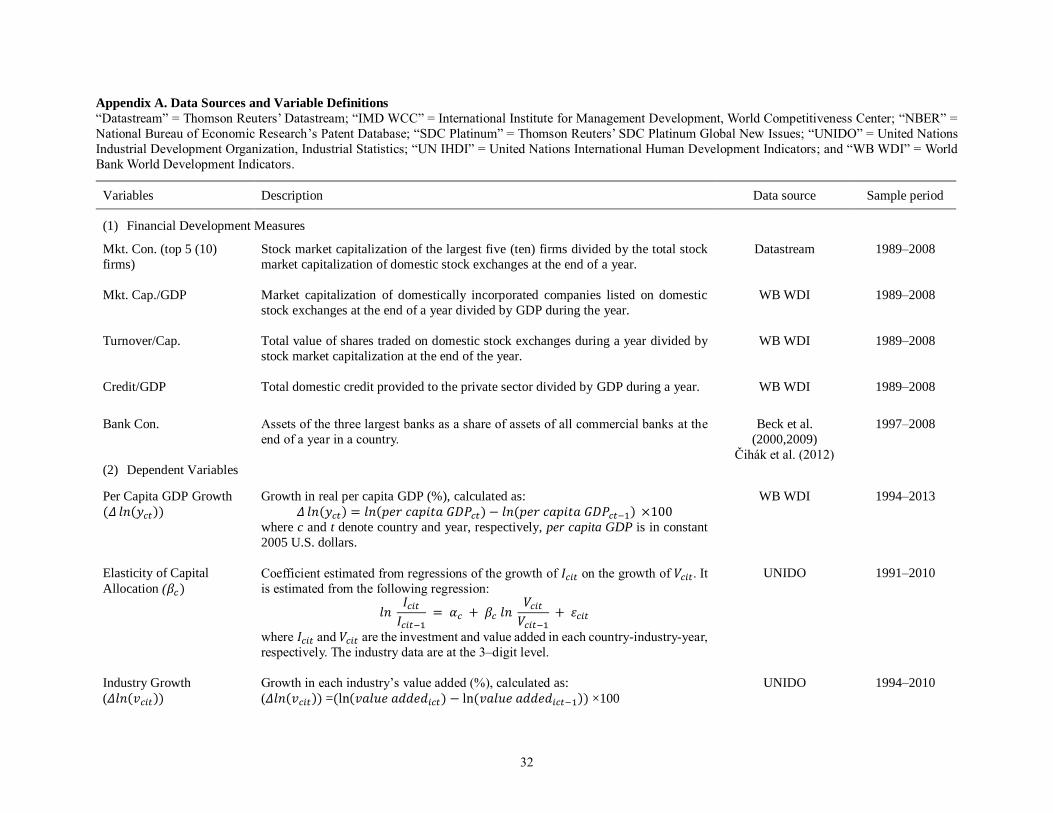
Appendix A. Data Sources and Variable Definitions
“Datastream” = Thomson Reuters’ Datastream; “IMD WCC” = International Institute for Management Development, World Competitiveness Center; “NBER” =
National Bureau of Economic Research’s Patent Database; “SDC Platinum” = Thomson Reuters’ SDC Platinum Global New Issues; “UNIDO” = United Nations
Industrial Development Organization, Industrial Statistics; “UN IHDI” = United Nations International Human Development Indicators; and “WB WDI” = World
Bank World Development Indicators.
Variables Description Data source Sample period
(1) Financial Development Measures
Mkt. Con. (top 5 (10)
firms)
Stock market capitalization of the largest five (ten) firms divided by the total stock
market capitalization of domestic stock exchanges at the end of a year.
Datastream 1989–2008
Mkt. Cap./GDP Market capitalization of domestically incorporated companies listed on domestic
stock exchanges at the end of a year divided by GDP during the year.
WB WDI 1989–2008
Turnover/Cap. Total value of shares traded on domestic stock exchanges during a year divided by
stock market capitalization at the end of the year.
WB WDI 1989–2008
Credit/GDP Total domestic credit provided to the private sector divided by GDP during a year.
WB WDI 1989–2008
Bank Con. Assets of the three largest banks as a share of assets of all commercial banks at the
end of a year in a country.
Beck et al.
(2000,2009)
Čihák et al. (2012)
1997–2008
(2) Dependent Variables
Per Capita GDP Growth
(𝛥 𝑙𝑛(𝑦𝑐𝑡))
Growth in real per capita GDP (%), calculated as:
𝛥 𝑙𝑛(𝑦𝑐𝑡) = 𝑙𝑛(𝑝𝑒𝑟 𝑐𝑎𝑝𝑖𝑡𝑎 𝐺𝐷𝑃𝑐𝑡) − 𝑙𝑛(𝑝𝑒𝑟 𝑐𝑎𝑝𝑖𝑡𝑎 𝐺𝐷𝑃𝑐𝑡−1) ×100
where c and t denote country and year, respectively, per capita GDP is in constant
2005 U.S. dollars.
WB WDI 1994–2013
Elasticity of Capital
Allocation (𝛽𝑐 )
Coefficient estimated from regressions of the growth of 𝐼𝑐𝑖𝑡 on the growth of 𝑉𝑐𝑖𝑡. It
is estimated from the following regression:
𝑙𝑛 𝐼𝑐𝑖𝑡
𝐼𝑐𝑖𝑡−1 = 𝛼𝑐 + 𝛽𝑐 𝑙𝑛
𝑉𝑐𝑖𝑡
𝑉𝑐𝑖𝑡−1 + 𝜀𝑐𝑖𝑡
where 𝐼𝑐𝑖𝑡 and 𝑉𝑐𝑖𝑡 are the investment and value added in each country-industry-year,
respectively. The industry data are at the 3–digit level.
UNIDO 1991–2010
Industry Growth
(𝛥𝑙𝑛(𝑣𝑐𝑖𝑡))
Growth in each industry’s value added (%), calculated as:
(𝛥𝑙𝑛(𝑣𝑐𝑖𝑡)) =(ln(𝑣𝑎𝑙𝑢𝑒 𝑎𝑑𝑑𝑒𝑑𝑖𝑐𝑡) − ln(𝑣𝑎𝑙𝑢𝑒 𝑎𝑑𝑑𝑒𝑑𝑖𝑐𝑡−1)) ×100
UNIDO 1994–2010
33
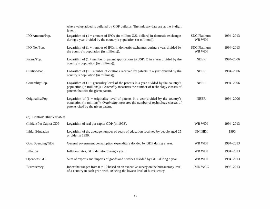
where value added is deflated by GDP deflator. The industry data are at the 3–digit
level.
IPO Amount/Pop. Logarithm of (1 + amount of IPOs (in million U.S. dollars) in domestic exchanges
during a year divided by the country’s population (in millions)).
SDC Platinum,
WB WDI
1994–2013
IPO No./Pop. Logarithm of (1 + number of IPOs in domestic exchanges during a year divided by
the country’s population (in millions)).
SDC Platinum,
WB WDI
1994–2013
Patent/Pop. Logarithm of (1 + number of patent applications to USPTO in a year divided by the
country’s population (in millions)).
NBER 1994–2006
Citation/Pop. Logarithm of (1 + number of citations received by patents in a year divided by the
country’s population (in millions)).
NBER 1994–2006
Generality/Pop.
Logarithm of (1 + generality level of the patents in a year divided by the country’s
population (in millions)). Generality measures the number of technology classes of
patents that cite the given patent.
NBER 1994–2006
Originality/Pop.
Logarithm of (1 + originality level of patents in a year divided by the country’s
population (in millions)). Originality measures the number of technology classes of
patents cited by the given patent.
NBER 1994–2006
(3) Control/Other Variables
(Initial) Per Capita GDP Logarithm of real per capita GDP (in 1993).
WB WDI 1994–2013
Initial Education Logarithm of the average number of years of education received by people aged 25
or older in 1990.
UN IHDI 1990
Gov. Spending/GDP General government consumption expenditure divided by GDP during a year.
WB WDI 1994–2013
Inflation Inflation rates, GDP deflator during a year.
WB WDI 1994–2013
Openness/GDP Sum of exports and imports of goods and services divided by GDP during a year.
WB WDI 1994–2013
Bureaucracy Index that ranges from 0 to 10 based on an executive survey on the bureaucracy level
of a country in each year, with 10 being the lowest level of bureaucracy.
IMD WCC 1995–2013

34
Corruption Index that ranges from 0 to 10 based on an executive survey on the bribery and
corruption level of a country in each year, with 10 being the lowest level of bribery
and corruption.
IMD WCC 1995–2013
Stability Index from 0 to 1 generated by counting the number of firms that stay in the top 5
(10) in both the current year and 5 years ago and dividing it by 5 (10).
Datastream 1994–2008
External Financing
Dependence
Median of external financing dependences of U.S. firms in each industry. A firm’s
external financing dependence is calculated as:
∑ Capital Expenditures𝑗𝑡 2010𝑡=1994 − ∑ Cash Flow from Operations𝑗𝑡
2010𝑡=1994
∑ Capital Expenditures𝑗𝑡 2010𝑡=1994
where j and t denote firm and year and each item is summed up for the period of
1994–2010.
Compustat 1994–2010
Equity Financing
Dependence
Median of equity financing dependences of U.S. firms in each industry. A firm’s
equity financing dependence is calculated as:
∑ Net Amount of Equity Issues𝑗𝑡
2010𝑡=1994
∑ Capital Expenditures𝑗𝑡 2010𝑡=1994
where j and t denote firm and year and each item is summed up for the period of
1994–2010.
Compustat 1994–2010
35
References
Acharya, V., Subramanian, K., 2009. Bankruptcy codes and innovation. Review of Financial
Studies 22, 4949–4988.
Aghion, P., Howitt, P., 1992. A model of growth through creative destruction. Econometrica 60,
323–351.
Aghion, P., Howitt, P., 1997. A Schumpeterian perspective on growth and competition. In: Krepts,
D., Wallis, K. (Eds.), Advances in Economics and Econometrics: Theory and Application,
pp. 279–317. Cambridge, UK: Cambridge University Press.
Aghion, P., Howitt, P., 1998. Endogenous Growth Theory. MIT Press, Cambridge, MA.
Arcand, L., Berkes, E., Panizza, U., 2011. Too much finance? IMF Working Paper, WP/12/161.
Beck, T., Degryse, H., Kneer, C., 2014. Is more finance better? Disentangling intermediation and
size effects of financial systems. Journal of Financial Stability 10, 50–64.
Beck, T., Demirgüç-Kunt, A., Levine, R., 2000. A New Database on Financial Development and
Structure. World Bank Economic Review 14, 597-605.
Beck, T., Demirgüç-Kunt, A., Levine, R., 2009. Financial Institutions and Markets across
Countries and over Time: Data and Analysis. World Bank Policy Research Working Paper
4943.
Beck, T., Levine, R., 2004. Stock markets, banks and growth: Panel evidence. Journal of Banking
and Finance 28, 423–442.
Beck, T., Levine, R., Loayza, N., 2000. Finance and the sources of growth. Journal of Financial
Economics 58, 261–300.
Bekaert, G., Harvey, C., Lundblad, C., 2005. Does Financial Liberalization Spur Growth? Journal
of Financial Economics 77, 3–55.
Cecchetti, S., Kharroubi, E., 2012. Reassessing the Impact of Finance on Growth. BIS Working
Paper Series, No. 381.
Cetorelli, N., Gambera, M., 2001. Banking market structure, financial dependence and growth:
International evidence from industry data. Journal of Finance 56, 617–648.
Čihák, M., Demirgüç-Kunt, A., Feyen, E., Levine, R., 2012. Benchmarking Financial
Development around the World. World Bank Policy Research Working Paper 6175.
Demirgüç-Kunt, A., Maksimovic, V., 1998. Law, finance, and firm growth. Journal of Finance 53,
2107–2137.
Doidge C., Karolyi, A., Stulz, R., 2013. The U.S. left behind? Financial globalization and the rise
of IPOs outside the U.S. Journal of Financial Economics 110, 546–573.

36
Doidge C., Karolyi, A., Stulz, R., 2016. The U.S. listing gap. Journal of Financial Economics.
Forthcoming.
Fogel, K., Morck, R., Yeung, B, 2008. Big business stability and economic growth: Is what’s good
for General Motors good for America? Journal of Financial Economics 89, 83–108.
Gabaix, X., 2011. The Granular Origins of Aggregate Fluctuations. Econometrica 79-3, 733–772.
Goldsmith, R., 1969. Financial Structure and Economic Development. New Haven, CT: Yale
University Press.
Grullon, G., Larkin, Y., Michaely, R., 2015. The disappearance of public firms and the changing
nature of U.S. industries. Working Paper.
Guiso, L., Sapienza, P., Zingales, L., 2004. Does local financial development matter? Quarterly
Journal of Economics 119, 929–969.
Hall, B., Jaffe, A., Trajtenberg, M., 2005. The NBER patent citation data file: Lessons, insights
and methodological tools. In: Jaffe, A., Trajtenberg, M. (Eds.), Patents, Citations and
Innovations: A Window on the Knowledge Economy. Cambridge, MA: MIT Press.
Hsu, P., Tian, X., Xu, Y., 2014. Financial development and innovation: Cross-country evidence.
Journal of Financial Economics 112(1), 116–135.
Jayaratne, J., Strahan, P., 1996. The finance–growth nexus: Evidence from bank branch
deregulation. Quarterly Journal of Economics 111, 639–670.
King, R., Levine, R., 1993. Finance and growth: Schumpeter might be right. Quarterly Journal of
Economics 108(3), 717–738.
La Porta, R., Lopez–de–Silanes, F., Shleifer, A., Vishny, R., 1997. Legal determinants of external
finance. Journal of Finance 52, 1131–1150.
Levine, R., 2005. Finance and growth: Theory and evidence. In: Aghion, P., Durlauf, S. (Eds.),
Handbook of Economic Growth, Vol. 1A. Amsterdam, Netherlands: Elsevier.
Levine, R., Zervos, S., 1998. Stock markets, banks, and economic growth. American Economic
Review 88, 537–558.
Lucas, R., 1988. On the mechanics of economic development. Journal of Monetary Economics,
22, 3–42.
McKinnon, R., 1973. Money and Capital in Economic Development. Washington, D.C.: Brooking
Institution.
Merton, R., Bodie, Z., 1995. A conceptual framework for analyzing the financial environment. In:
D. B. Crane, et al. (Eds.), The Global Financial System: A Functional Perspective.
Cambridge, MA: Harvard Business School Press.
37
Mian, A., Sufi, A., 2014. House of Debt: How They (and You) Caused the Great Recession, and
How We Can Prevent it from Happening Again. Chicago, IL: University of Chicago Press.
Miller, M., 1998. Financial markets and economic growth. Journal of Applied Corporate Finance
11, 8–14.
Nelson, R., Winter, S., 1982. An Evolutionary Theory of Economic Change. Cambridge, MA:
Harvard University Press.
Petersen, M., 2009. Estimating standard errors in finance panel data sets: Comparing approaches.
Review of Financial Studies 22, 435–480.
Rajan, R., Zingales, L., 1998. Financial dependence and growth. American Economic Review 88,
559–586.
Rajan, R., Zingales, L., 2003. Saving Capitalism from Capitalists: Unleashing the Power of
Financial Markets to Create Wealth and Spread Opportunity. New York: Crown Business.
Robinson, J., 1952. The generalization of the general theory. In: The Rate of Interest and Other
Essays. London: MacMillan.
Rousseau, P., Wachtel, P., 2000. Equity markets and growth: Cross-country evidence on timing
and outcomes, 1980–1995. Journal of Business and Finance 24, 1933–1957.
Schularick, M., Taylor, A., 2012. Credit booms gone bust: Monetary policy, leverage cycles, and
financial crises, 1870–2008. American Economic Review 102(2), 1029–1061.
Schumpeter, J., 1912. Theorie der Wirtschaftlichen Entwichlung. Leipzig, Dunker und Humbolt.
Translated by Opie, R. (1934). The Theory of Economic Development: An Inquiry into
Profits, Capital, Credit, Interest, and Business Cycle. Cambridge, MA: Harvard University
Press.
United Nations Industrial Development Organization, 2014. International Yearbook of Industrial
Statistics (20th Edition). New York: United Nations.
Wurgler, J., 2000. Financial markets and the allocation of capital. Journal of Financial Economics
58, 187–214.
Zingales, L., 2003. Commentary on more finance more growth. The Federal Reserve of St. Louis
Review.
Zingales, L., 2015. Presidential address: Does finance benefit society? Journal of Finance 70,
1327–1363.

38
Figure 1
Average Stock Market Concentration by Year
Figure 1 plots the average stock market concentration computed using the top five (ten) firms in each year during
1989–2008.
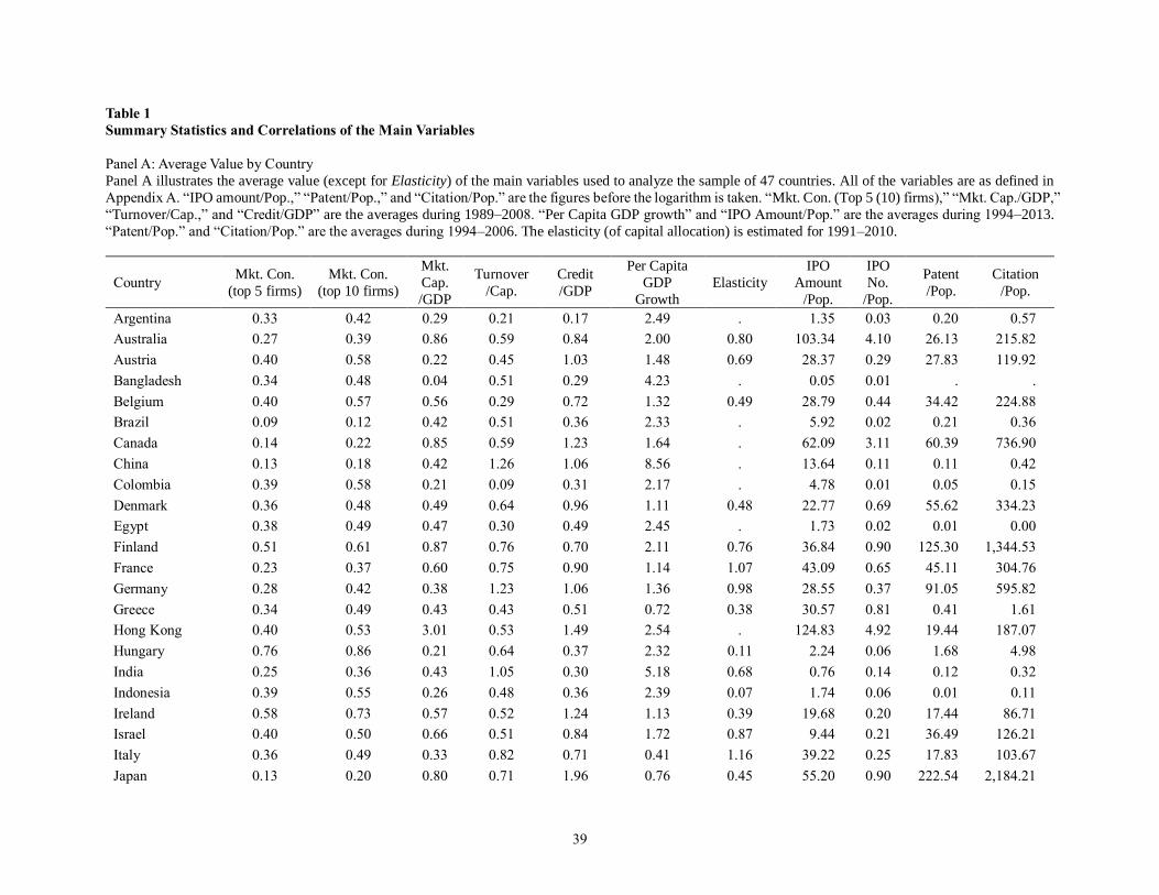
39
Table 1
Summary Statistics and Correlations of the Main Variables
Panel A: Average Value by Country
Panel A illustrates the average value (except for Elasticity) of the main variables used to analyze the sample of 47 countries. All of the variables are as defined in
Appendix A. “IPO amount/Pop.,” “Patent/Pop.,” and “Citation/Pop.” are the figures before the logarithm is taken. “Mkt. Con. (Top 5 (10) firms),” “Mkt. Cap./GDP,”
“Turnover/Cap.,” and “Credit/GDP” are the averages during 1989–2008. “Per Capita GDP growth” and “IPO Amount/Pop.” are the averages during 1994–2013.
“Patent/Pop.” and “Citation/Pop.” are the averages during 1994–2006. The elasticity (of capital allocation) is estimated for 1991–2010.
Country Mkt. Con.
(top 5 firms)
Mkt. Con.
(top 10 firms)
Mkt.
Cap.
/GDP
Turnover
/Cap.
Credit
/GDP
Per Capita
GDP
Growth
Elasticity
IPO
Amount
/Pop.
IPO
No.
/Pop.
Patent
/Pop.
Citation
/Pop.
Argentina 0.33 0.42 0.29 0.21 0.17 2.49 . 1.35 0.03 0.20 0.57
Australia 0.27 0.39 0.86 0.59 0.84 2.00 0.80 103.34 4.10 26.13 215.82
Austria 0.40 0.58 0.22 0.45 1.03 1.48 0.69 28.37 0.29 27.83 119.92
Bangladesh 0.34 0.48 0.04 0.51 0.29 4.23 . 0.05 0.01 . .
Belgium 0.40 0.57 0.56 0.29 0.72 1.32 0.49 28.79 0.44 34.42 224.88
Brazil 0.09 0.12 0.42 0.51 0.36 2.33 . 5.92 0.02 0.21 0.36
Canada 0.14 0.22 0.85 0.59 1.23 1.64 . 62.09 3.11 60.39 736.90
China 0.13 0.18 0.42 1.26 1.06 8.56 . 13.64 0.11 0.11 0.42
Colombia 0.39 0.58 0.21 0.09 0.31 2.17 . 4.78 0.01 0.05 0.15
Denmark 0.36 0.48 0.49 0.64 0.96 1.11 0.48 22.77 0.69 55.62 334.23
Egypt 0.38 0.49 0.47 0.30 0.49 2.45 . 1.73 0.02 0.01 0.00
Finland 0.51 0.61 0.87 0.76 0.70 2.11 0.76 36.84 0.90 125.30 1,344.53
France 0.23 0.37 0.60 0.75 0.90 1.14 1.07 43.09 0.65 45.11 304.76
Germany 0.28 0.42 0.38 1.23 1.06 1.36 0.98 28.55 0.37 91.05 595.82
Greece 0.34 0.49 0.43 0.43 0.51 0.72 0.38 30.57 0.81 0.41 1.61
Hong Kong 0.40 0.53 3.01 0.53 1.49 2.54 . 124.83 4.92 19.44 187.07
Hungary 0.76 0.86 0.21 0.64 0.37 2.32 0.11 2.24 0.06 1.68 4.98
India 0.25 0.36 0.43 1.05 0.30 5.18 0.68 0.76 0.14 0.12 0.32
Indonesia 0.39 0.55 0.26 0.48 0.36 2.39 0.07 1.74 0.06 0.01 0.11
Ireland 0.58 0.73 0.57 0.52 1.24 1.13 0.39 19.68 0.20 17.44 86.71
Israel 0.40 0.50 0.66 0.51 0.84 1.72 0.87 9.44 0.21 36.49 126.21
Italy 0.36 0.49 0.33 0.82 0.71 0.41 1.16 39.22 0.25 17.83 103.67
Japan 0.13 0.20 0.80 0.71 1.96 0.76 0.45 55.20 0.90 222.54 2,184.21
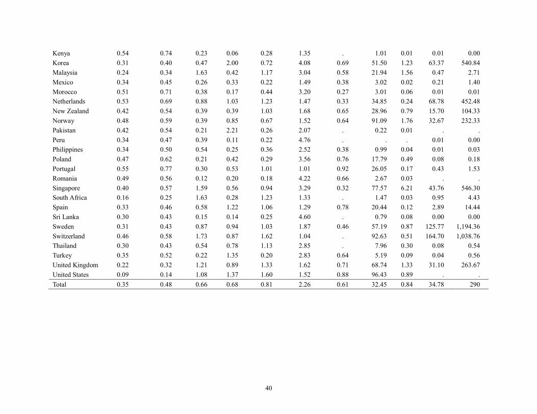
40
Kenya 0.54 0.74 0.23 0.06 0.28 1.35 . 1.01 0.01 0.01 0.00
Korea 0.31 0.40 0.47 2.00 0.72 4.08 0.69 51.50 1.23 63.37 540.84
Malaysia 0.24 0.34 1.63 0.42 1.17 3.04 0.58 21.94 1.56 0.47 2.71
Mexico 0.34 0.45 0.26 0.33 0.22 1.49 0.38 3.02 0.02 0.21 1.40
Morocco 0.51 0.71 0.38 0.17 0.44 3.20 0.27 3.01 0.06 0.01 0.01
Netherlands 0.53 0.69 0.88 1.03 1.23 1.47 0.33 34.85 0.24 68.78 452.48
New Zealand 0.42 0.54 0.39 0.39 1.03 1.68 0.65 28.96 0.79 15.70 104.33
Norway 0.48 0.59 0.39 0.85 0.67 1.52 0.64 91.09 1.76 32.67 232.33
Pakistan 0.42 0.54 0.21 2.21 0.26 2.07 . 0.22 0.01 . .
Peru 0.34 0.47 0.39 0.11 0.22 4.76 . . . 0.01 0.00
Philippines 0.34 0.50 0.54 0.25 0.36 2.52 0.38 0.99 0.04 0.01 0.03
Poland 0.47 0.62 0.21 0.42 0.29 3.56 0.76 17.79 0.49 0.08 0.18
Portugal 0.55 0.77 0.30 0.53 1.01 1.01 0.92 26.05 0.17 0.43 1.53
Romania 0.49 0.56 0.12 0.20 0.18 4.22 0.66 2.67 0.03 . .
Singapore 0.40 0.57 1.59 0.56 0.94 3.29 0.32 77.57 6.21 43.76 546.30
South Africa 0.16 0.25 1.63 0.28 1.23 1.33 . 1.47 0.03 0.95 4.43
Spain 0.33 0.46 0.58 1.22 1.06 1.29 0.78 20.44 0.12 2.89 14.44
Sri Lanka 0.30 0.43 0.15 0.14 0.25 4.60 . 0.79 0.08 0.00 0.00
Sweden 0.31 0.43 0.87 0.94 1.03 1.87 0.46 57.19 0.87 125.77 1,194.36
Switzerland 0.46 0.58 1.73 0.87 1.62 1.04 . 92.63 0.51 164.70 1,038.76
Thailand 0.30 0.43 0.54 0.78 1.13 2.85 . 7.96 0.30 0.08 0.54
Turkey 0.35 0.52 0.22 1.35 0.20 2.83 0.64 5.19 0.09 0.04 0.56
United Kingdom 0.22 0.32 1.21 0.89 1.33 1.62 0.71 68.74 1.33 31.10 263.67
United States 0.09 0.14 1.08 1.37 1.60 1.52 0.88 96.43 0.89 . .
Total 0.35 0.48 0.66 0.68 0.81 2.26 0.61 32.45 0.84 34.78 290

41
Panel B: Correlations
Panel B presents Pearson’s correlations among the main variables. The sample includes country-year observations for 47 countries during 1994–2013 except for
the elasticity of capital allocation, which is estimated for 1991–2010, and “Patent/Pop.” and “Citation/Pop.,” whose data are collected for 1994–2006. The asterisks
denote statistical significance at or below the 5% level.
Variables [1] [2] [3] [4] [5] [6] [7] [8] [9] [10] [11]
[1] Mkt. Con. (top 5 firms) at t–5 1.00
[2] Mkt. Con. (top 10 firms) at t–5 0.97* 1.00
[3] Mkt. Cap./GDP at t–5 –0.04 –0.07* 1.00
[4] Turnover/Cap. at t–5 –0.03 –0.05 0.04 1.00
[5] Credit/GDP at t–5 –0.20* –0.21* 0.52* 0.25* 1.00
[6] Per Capita GDP Growth –0.14* –0.16* –0.11* –0.04 –0.23* 1.00
[7] Elasticity of Capital Allocation –0.29* –0.30* –0.03 0.21* 0.18* –0.07 1.00
[8] IPO Amount/Pop. –0.24* –0.25* 0.25* 0.03 0.33* 0.21* 0.22* 1.00
[9] IPO No./Pop. –0.18* –0.18* 0.36* –0.05 0.26* 0.15* 0.03 0.74* 1.00
[10] Patent/Pop. –0.13* –0.18* 0.16* 0.01 0.45* –0.11* 0.19* 0.47* 0.43* 1.00
[11] Citation/Pop. –0.20* –0.24* 0.11* –0.04 0.40* –0.09* 0.19* 0.47* 0.45* 0.97* 1.00
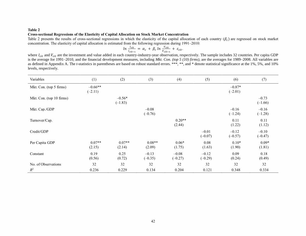
42
Table 2
Cross-sectional Regressions of the Elasticity of Capital Allocation on Stock Market Concentration
Table 2 presents the results of cross-sectional regressions in which the elasticity of the capital allocation of each country (𝛽𝑐 ) are regressed on stock market
concentration. The elasticity of capital allocation is estimated from the following regression during 1991–2010:
𝑙𝑛 𝐼𝑐𝑖𝑡
𝐼𝑐𝑖𝑡−1 = 𝛼𝑐 + 𝛽𝑐 𝑙𝑛
𝑉𝑐𝑖𝑡
𝑉𝑐𝑖𝑡−1 + 𝜀𝑐𝑖𝑡.
where 𝐼𝑐𝑖𝑡 and 𝑉𝑐𝑖𝑡 are the investment and value added in each country-industry-year observation, respectively. The sample includes 32 countries. Per capita GDP
is the average for 1991–2010, and the financial development measures, including Mkt. Con. (top 5 (10) firms), are the averages for 1989–2008. All variables are
as defined in Appendix A. The t-statistics in parentheses are based on robust standard errors. ***, **, and * denote statistical significance at the 1%, 5%, and 10%
levels, respectively.
Variables (1) (2) (3) (4) (5) (6) (7)
Mkt. Con. (top 5 firms) –0.66** –0.87*
(–2.11) (–2.01)
Mkt. Con. (top 10 firms) –0.56* –0.73
(–1.83) (–1.66)
Mkt. Cap./GDP –0.08 –0.16 –0.16
(–0.76) (–1.24) (–1.28)
Turnover/Cap. 0.20** 0.11 0.11
(2.44) (1.22) (1.12)
Credit/GDP –0.01 –0.12 –0.10
(–0.07) (–0.57) (–0.47)
Per Capita GDP 0.07** 0.07** 0.08** 0.06* 0.08 0.10* 0.09*
(2.15) (2.14) (2.09) (1.75) (1.63) (1.90) (1.81)
Constant 0.19 0.25 –0.13 –0.08 –0.12 0.09 0.18
(0.56) (0.72) (–0.35) (–0.27) (–0.29) (0.24) (0.49)
No. of Observations 32 32 32 32 32 32 32
R2 0.236 0.229 0.134 0.204 0.121 0.348 0.334

43
Table 3
Panel Regressions of Per Capita GDP Growth on Stock Market Concentration at t–5
Table 3 presents the results of the panel regressions in which per capita GDP growth rates are regressed on stock market concentration at t–5. This sample includes
country-year observations for 47 countries during 1994–2013. All variables are as defined in Appendix A. The t-statistics in parentheses are based on standard
errors clustered by both year and country (panel A) and by country (panel B). ***, **, and * denote statistical significance at the 1%, 5%, and 10% levels,
respectively.
Panel A. Pooled OLS Regressions of Per Capita GDP Growth on Stock Market Concentration at t–5
Variables (1) (2) (3) (4) (5) (6)
Mkt. Con. (top 5 firms) at t–5 –3.98*** –4.27***
(–3.44) (–3.42)
Mkt. Con. (top 10 firms) at t–5 –3.88*** –4.23***
(–3.57) (–3.61)
Mkt. Cap./GDP at t–5 –0.50 –0.63 –0.72*
(–1.41) (–1.62) (–1.78)
Turnover/Cap. at t–5 0.16 0.21 0.18
(0.77) (1.09) (0.98)
Credit/GDP at t–5 –1.39*** –1.45*** –0.66 –0.99** –1.14*** –1.16***
(–3.24) (–3.62) (–1.14) (–2.06) (–2.98) (–3.21)
Initial Per Capita GDP –0.54 –0.53* –0.54 –0.55 –0.54* –0.52*
(–1.64) (–1.69) (–1.49) (–1.49) (–1.69) (–1.74)
Initial Education 1.07** 0.91* 1.11** 1.17** 1.15** 0.97*
(2.23) (1.95) (2.43) (2.42) (2.23) (1.93)
Gov. Spending/GDP –7.51* –6.70* –11.57*** –10.77*** –8.40** –7.67*
(–1.93) (–1.68) (–2.89) (–2.59) (–2.24) (–1.96)
Inflation –0.03 –0.03 –0.03 –0.03 –0.03 –0.03
(–1.34) (–1.33) (–1.27) (–1.30) (–1.37) (–1.35)
Openness/GDP 0.57*** 0.64*** 0.43*** 0.23 0.88*** 1.00***
(3.69) (3.84) (3.14) (1.40) (4.41) (4.37)
Constant 8.53*** 9.01*** 7.48*** 7.41*** 8.40*** 8.95***
(4.31) (4.55) (3.67) (3.68) (4.47) (4.78)
No. of Observations 834 834 834 832 832 832
R2 0.170 0.178 0.142 0.137 0.181 0.192

44
Panel B. Country Fixed Effects Regressions of Per Capita GDP Growth on Stock Market Concentration at t–5
Variables (1) (2) (3) (4) (5) (6)
Mkt. Con. (top 5 firms) at t–5 –4.19*** –3.66**
(–3.00) (–2.41)
Mkt. Con. (top 10 firms) at t–5 –4.11*** –3.79***
(–3.26) (–2.77)
Mkt. Cap./GDP at t–5 –1.17** –1.05** –1.06**
(–2.69) (–2.19) (–2.21)
Turnover/Cap. at t–5 –0.05 0.01 0.02
(–0.24) (0.04) (0.12)
Credit/GDP at t–5 –1.85*** –1.82*** –1.81*** –1.88*** –1.77*** –1.74***
(–3.48) (–3.48) (–3.39) (–3.33) (–3.21) (–3.22)
Gov. Spending/GDP –60.07*** –58.47*** –62.60*** –63.71*** –59.16*** –57.53***
(–3.52) (–3.46) (–3.59) (–3.64) (–3.39) (–3.33)
Inflation –0.05 –0.05 –0.05 –0.05 –0.05 –0.05
(–1.39) (–1.40) (–1.34) (–1.34) (–1.37) (–1.39)
Openness/GDP 1.72** 1.71** 2.39** 1.19* 2.68** 2.70**
(2.45) (2.50) (2.35) (1.74) (2.57) (2.60)
Constant 11.78*** 11.92*** 10.84*** 11.01*** 11.49*** 11.66***
(5.52) (5.71) (5.17) (5.26) (5.19) (5.39)
Country Fixed Effects Yes Yes Yes Yes Yes Yes
No. of Observations 834 834 834 832 832 832
R2 0.325 0.326 0.327 0.311 0.336 0.338
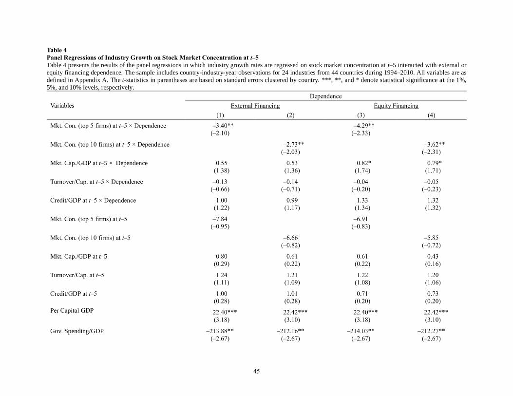
45
Table 4
Panel Regressions of Industry Growth on Stock Market Concentration at t–5
Table 4 presents the results of the panel regressions in which industry growth rates are regressed on stock market concentration at t–5 interacted with external or
equity financing dependence. The sample includes country-industry-year observations for 24 industries from 44 countries during 1994–2010. All variables are as
defined in Appendix A. The t-statistics in parentheses are based on standard errors clustered by country. ***, **, and * denote statistical significance at the 1%,
5%, and 10% levels, respectively.
Variables
Dependence
External Financing Equity Financing
(1) (2) (3) (4)
Mkt. Con. (top 5 firms) at t–5 × Dependence –3.40** –4.29**
(–2.10) (–2.33)
Mkt. Con. (top 10 firms) at t–5 × Dependence –2.73** –3.62**
(–2.03) (–2.31)
Mkt. Cap./GDP at t–5 × Dependence 0.55 0.53 0.82* 0.79*
(1.38) (1.36) (1.74) (1.71)
Turnover/Cap. at t–5 × Dependence –0.13 –0.14 –0.04 –0.05
(–0.66) (–0.71) (–0.20) (–0.23)
Credit/GDP at t–5 × Dependence 1.00 0.99 1.33 1.32
(1.22) (1.17) (1.34) (1.32)
Mkt. Con. (top 5 firms) at t–5 –7.84 –6.91
(–0.95) (–0.83)
Mkt. Con. (top 10 firms) at t–5 –6.66 –5.85
(–0.82) (–0.72)
Mkt. Cap./GDP at t–5 0.80 0.61 0.61 0.43
(0.29) (0.22) (0.22) (0.16)
Turnover/Cap. at t–5 1.24 1.21 1.22 1.20
(1.11) (1.09) (1.08) (1.06)
Credit/GDP at t–5 1.00 1.01 0.71 0.73
(0.28) (0.28) (0.20) (0.20)
Per Capital GDP 22.40*** 22.42*** 22.40*** 22.42***
(3.18) (3.10) (3.18) (3.10)
Gov. Spending/GDP –213.88** –212.16** –214.03** –212.27**
(–2.67) (–2.67) (–2.67) (–2.67)
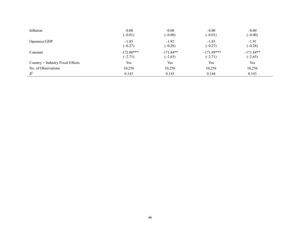
46
Inflation –0.00 –0.00 –0.00 –0.00
(–0.01) (–0.00) (–0.01) (–0.00)
Openness/GDP –1.85 –1.92 –1.83 –1.91
(–0.27) (–0.28) (–0.27) (–0.28)
Constant –172.00*** –171.84** –171.99*** –171.84**
(–2.71) (–2.65) (–2.71) (–2.65)
Country × Industry Fixed Effects Yes Yes Yes Yes
No. of Observations 10,256 10,256 10,256 10,256
R2 0.143 0.143 0.144 0.143
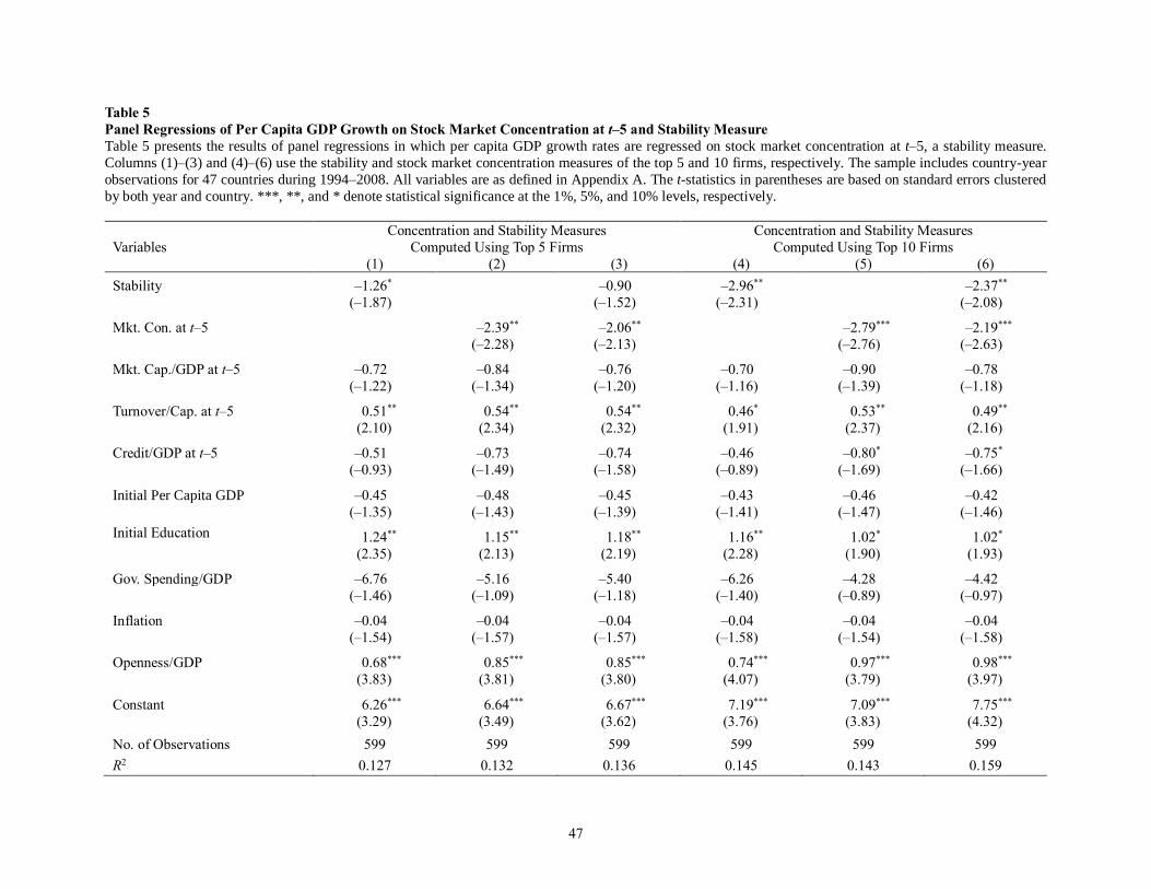
47
Table 5
Panel Regressions of Per Capita GDP Growth on Stock Market Concentration at t–5 and Stability Measure
Table 5 presents the results of panel regressions in which per capita GDP growth rates are regressed on stock market concentration at t–5, a stability measure.
Columns (1)–(3) and (4)–(6) use the stability and stock market concentration measures of the top 5 and 10 firms, respectively. The sample includes country-year
observations for 47 countries during 1994–2008. All variables are as defined in Appendix A. The t-statistics in parentheses are based on standard errors clustered
by both year and country. ***, **, and * denote statistical significance at the 1%, 5%, and 10% levels, respectively.
Variables
Concentration and Stability Measures
Computed Using Top 5 Firms
Concentration and Stability Measures
Computed Using Top 10 Firms
(1) (2) (3) (4) (5) (6)
Stability –1.26* –0.90 –2.96** –2.37**
(–1.87) (–1.52) (–2.31) (–2.08)
Mkt. Con. at t–5 –2.39** –2.06** –2.79*** –2.19***
(–2.28) (–2.13) (–2.76) (–2.63)
Mkt. Cap./GDP at t–5 –0.72 –0.84 –0.76 –0.70 –0.90 –0.78
(–1.22) (–1.34) (–1.20) (–1.16) (–1.39) (–1.18)
Turnover/Cap. at t–5 0.51** 0.54** 0.54** 0.46* 0.53** 0.49**
(2.10) (2.34) (2.32) (1.91) (2.37) (2.16)
Credit/GDP at t–5 –0.51 –0.73 –0.74 –0.46 –0.80* –0.75*
(–0.93) (–1.49) (–1.58) (–0.89) (–1.69) (–1.66)
Initial Per Capita GDP –0.45 –0.48 –0.45 –0.43 –0.46 –0.42
(–1.35) (–1.43) (–1.39) (–1.41) (–1.47) (–1.46)
Initial Education 1.24** 1.15** 1.18** 1.16** 1.02* 1.02*
(2.35) (2.13) (2.19) (2.28) (1.90) (1.93)
Gov. Spending/GDP –6.76 –5.16 –5.40 –6.26 –4.28 –4.42
(–1.46) (–1.09) (–1.18) (–1.40) (–0.89) (–0.97)
Inflation –0.04 –0.04 –0.04 –0.04 –0.04 –0.04
(–1.54) (–1.57) (–1.57) (–1.58) (–1.54) (–1.58)
Openness/GDP 0.68*** 0.85*** 0.85*** 0.74*** 0.97*** 0.98***
(3.83) (3.81) (3.80) (4.07) (3.79) (3.97)
Constant 6.26*** 6.64*** 6.67*** 7.19*** 7.09*** 7.75***
(3.29) (3.49) (3.62) (3.76) (3.83) (4.32)
No. of Observations 599 599 599 599 599 599
R2 0.127 0.132 0.136 0.145 0.143 0.159
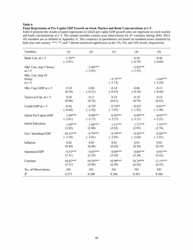
48
Table 6
Panel Regressions of Per Capita GDP Growth on Stock Market and Bank Concentrations at t–5
Table 6 presents the results of panel regressions in which per capita GDP growth rates are regressed on stock market
and bank concentrations at t–5. The sample includes country-year observations for 47 countries during 2002–2013.
All variables are as defined in Appendix A. The t-statistics in parentheses are based on standard errors clustered by
both year and country. ***, **, and * denote statistical significance at the 1%, 5%, and 10% levels, respectively.
Variables (1) (2) (3) (4) (5)
Bank Con. at t–5 –1.29** –0.56 –0.46
(–2.01) (–0.79) (–0.60)
Mkt. Con. (top 5 firms) –3.98*** –3.82***
at t–5 (–3.93) (–3.55)
Mkt. Con. (top 10
firms) –3.75*** –3.64***
at t–5 (–3.73) (–3.29)
Mkt. Cap./GDP at t–5 0.10 –0.06 –0.14 –0.06 –0.13
(0.39) (–0.21) (–0.47) (–0.18) (–0.44)
Turnover/Cap. at t–5 0.20 0.17 0.14 0.19 0.15
(0.80) (0.76) (0.61) (0.79) (0.63)
Credit/GDP at t–5 –0.38 –0.79* –0.79** –0.82* –0.81**
(–0.68) (–1.92) (–1.97) (–1.92) (–1.98)
Initial Per Capita GDP –1.04*** –0.99*** –0.95*** –0.99*** –0.95***
(–2.81) (–3.17) (–3.27) (–3.11) (–3.21)
Initial Education 1.69*** 1.68*** 1.51*** 1.71*** 1.53***
(3.02) (2.88) (2.65) (2.95) (2.74)
Gov. Spending/GDP –10.53*** –8.79*** –8.79*** –8.56*** –8.60***
(–3.39) (–3.01) (–2.95) (–2.94) (–2.91)
Inflation 0.02 0.01 0.01 0.01 0.01
(0.49) (0.44) (0.24) (0.36) (0.19)
Openness/GDP 0.53*** 0.83*** 0.89*** 0.86*** 0.91***
(3.31) (5.23) (5.24) (5.34) (5.52)
Constant 10.42*** 10.54*** 10.99*** 10.76*** 11.15***
(5.51) (5.96) (6.20) (6.26) (6.53)
No. of Observations 541 541 541 541 541
R2 0.273 0.300 0.306 0.301 0.306
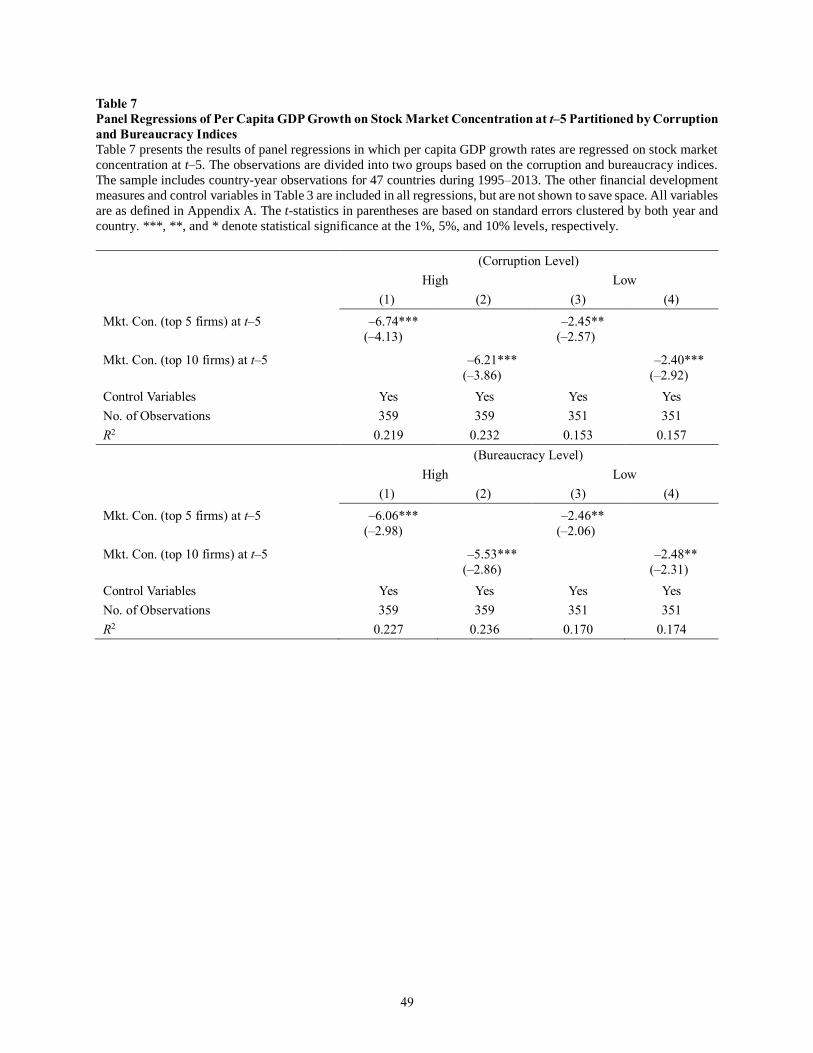
49
Table 7
Panel Regressions of Per Capita GDP Growth on Stock Market Concentration at t–5 Partitioned by Corruption
and Bureaucracy Indices
Table 7 presents the results of panel regressions in which per capita GDP growth rates are regressed on stock market
concentration at t–5. The observations are divided into two groups based on the corruption and bureaucracy indices.
The sample includes country-year observations for 47 countries during 1995–2013. The other financial development
measures and control variables in Table 3 are included in all regressions, but are not shown to save space. All variables
are as defined in Appendix A. The t-statistics in parentheses are based on standard errors clustered by both year and
country. ***, **, and * denote statistical significance at the 1%, 5%, and 10% levels, respectively.
(Corruption Level)
High Low
(1) (2) (3) (4)
Mkt. Con. (top 5 firms) at t–5
–6.74*** –2.45**
(–4.13) (–2.57)
Mkt. Con. (top 10 firms) at t–5
–6.21*** –2.40***
(–3.86) (–2.92)
Control Variables Yes Yes Yes Yes
No. of Observations 359 359 351 351
R2 0.219 0.232 0.153 0.157
(Bureaucracy Level)
High Low
(1) (2) (3) (4)
Mkt. Con. (top 5 firms) at t–5
–6.06*** –2.46**
(–2.98) (–2.06)
Mkt. Con. (top 10 firms) at t–5
–5.53*** –2.48**
(–2.86) (–2.31)
Control Variables Yes Yes Yes Yes
No. of Observations 359 359 351 351
R2 0.227 0.236 0.170 0.174
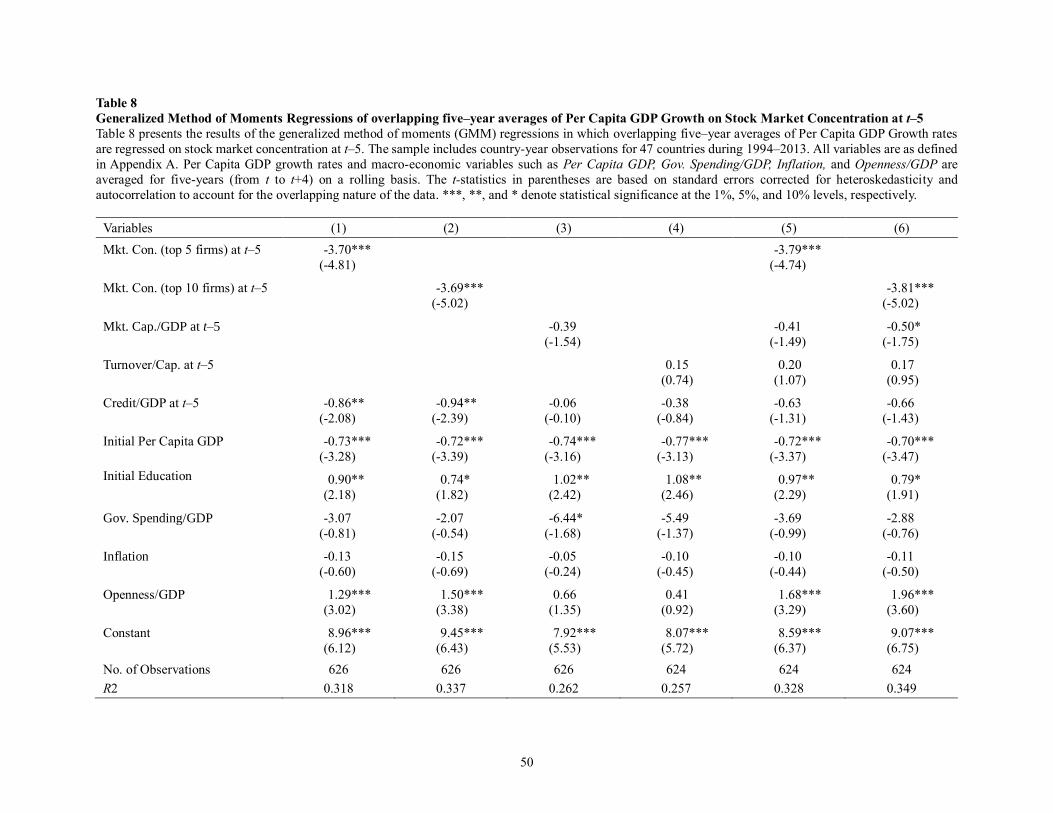
50
Table 8
Generalized Method of Moments Regressions of overlapping five–year averages of Per Capita GDP Growth on Stock Market Concentration at t–5
Table 8 presents the results of the generalized method of moments (GMM) regressions in which overlapping five–year averages of Per Capita GDP Growth rates
are regressed on stock market concentration at t–5. The sample includes country-year observations for 47 countries during 1994–2013. All variables are as defined
in Appendix A. Per Capita GDP growth rates and macro-economic variables such as Per Capita GDP, Gov. Spending/GDP, Inflation, and Openness/GDP are
averaged for five-years (from t to t+4) on a rolling basis. The t-statistics in parentheses are based on standard errors corrected for heteroskedasticity and
autocorrelation to account for the overlapping nature of the data. ***, **, and * denote statistical significance at the 1%, 5%, and 10% levels, respectively.
Variables (1) (2) (3) (4) (5) (6)
Mkt. Con. (top 5 firms) at t–5 -3.70*** -3.79***
(-4.81) (-4.74)
Mkt. Con. (top 10 firms) at t–5 -3.69*** -3.81***
(-5.02) (-5.02)
Mkt. Cap./GDP at t–5 -0.39 -0.41 -0.50*
(-1.54) (-1.49) (-1.75)
Turnover/Cap. at t–5 0.15 0.20 0.17
(0.74) (1.07) (0.95)
Credit/GDP at t–5 -0.86** -0.94** -0.06 -0.38 -0.63 -0.66
(-2.08) (-2.39) (-0.10) (-0.84) (-1.31) (-1.43)
Initial Per Capita GDP -0.73*** -0.72*** -0.74*** -0.77*** -0.72*** -0.70***
(-3.28) (-3.39) (-3.16) (-3.13) (-3.37) (-3.47)
Initial Education 0.90** 0.74* 1.02** 1.08** 0.97** 0.79*
(2.18) (1.82) (2.42) (2.46) (2.29) (1.91)
Gov. Spending/GDP -3.07 -2.07 -6.44* -5.49 -3.69 -2.88
(-0.81) (-0.54) (-1.68) (-1.37) (-0.99) (-0.76)
Inflation -0.13 -0.15 -0.05 -0.10 -0.10 -0.11
(-0.60) (-0.69) (-0.24) (-0.45) (-0.44) (-0.50)
Openness/GDP 1.29*** 1.50*** 0.66 0.41 1.68*** 1.96***
(3.02) (3.38) (1.35) (0.92) (3.29) (3.60)
Constant 8.96*** 9.45*** 7.92*** 8.07*** 8.59*** 9.07***
(6.12) (6.43) (5.53) (5.72) (6.37) (6.75)
No. of Observations 626 626 626 624 624 624
R2 0.318 0.337 0.262 0.257 0.328 0.349

51
Table 9
Panel Regressions of IPO Activity on Stock Market Concentration at t–5
Table 9 presents the results of panel regressions in which measures of IPO activity are regressed on stock market
concentration at t–5. The sample includes country-year observations for 46 countries during 1994–2013. All variables
are as defined in Appendix A. The t-statistics in parentheses are based on standard errors clustered by country. ***,
**, and * denote statistical significance at the 1%, 5%, and 10% levels, respectively.
Dependent Variable IPO Amount/Pop. IPO No./Pop.
(1) (2) (3) (4)
Mkt. Con. (top 5 firms) at t–5 –1.09** –0.24
(–2.05) (–1.63)
Mkt. Con. (top 10 firms) at t–5 –1.20** –0.29**
(–2.26) (–2.13)
Mkt. Cap./GDP at t–5 –0.68*** –0.68*** –0.21*** –0.21***
(–4.16) (–4.24) (–3.56) (–3.62)
Turnover/Cap. at t–5 –0.23** –0.23** –0.06* –0.05
(–2.03) (–2.02) (–1.68) (–1.66)
Credit/GDP at t–5 –1.26*** –1.25*** –0.20** –0.20**
(–3.40) (–3.40) (–2.07) (–2.06)
Per Capita GDP 1.21*** 1.23*** 0.05 0.06
(3.18) (3.27) (0.33) (0.39)
Gov. Spending/GDP –27.25*** –26.71*** –4.17*** –4.03***
(–5.23) (–5.06) (–2.83) (–2.73)
Inflation –0.02*** –0.02*** –0.00*** –0.00***
(–5.67) (–5.73) (–3.08) (–3.13)
Openness/GDP 0.36 0.37 0.10 0.10
(1.03) (1.04) (0.65) (0.66)
Constant –5.54 –5.71 0.29 0.24
(–1.58) (–1.64) (0.21) (0.18)
Country Fixed Effects Yes Yes Yes Yes
No. of Observations 820 820 820 820
R2 0.571 0.572 0.725 0.726

52
Table 10
Panel Regressions of Innovation on Stock Market Concentration at t–5
Table 10 presents the results of panel regressions in which measures of innovation are regressed on stock market concentration at t–5. The sample includes country-
year observations for 43 countries during 1994–2006. All variables are as defined in Appendix A. The t-statistics in parentheses are based on standard errors
clustered by country. ***, **, and * denote statistical significance at the 1%, 5%, and 10% levels, respectively.
Dependent Variable Patent/Pop. Citation /Pop. Generality/Pop. Originality/Pop.
(1) (2) (3) (4) (5) (6) (7) (8)
Mkt. Con. (top 5 firms) at t–5 –2.39** –4.60*** –2.97*** –2.12**
(–2.58) (–3.04) (–3.78) (–2.58)
Mkt. Con. (top 10 firms) at t–5 –2.52*** –4.90*** –3.13*** –2.24***
(–2.97) (–3.56) (–4.46) (–3.01)
Mkt. Cap./GDP at t–5 –0.40* –0.40** –1.05** –1.03** –0.85*** –0.84*** –0.41** –0.40**
(–2.01) (–2.10) (–2.31) (–2.42) (–2.91) (–3.10) (–2.15) (–2.24)
Turnover/Cap. at t–5 –0.28* –0.27* –0.47* –0.46* –0.17 –0.17 –0.25* –0.24*
(–1.95) (–1.97) (–1.84) (–1.87) (–1.21) (–1.21) (–1.99) (–2.01)
Credit/GDP at t–5 –1.11* –1.05* –1.86* –1.76* –0.68 –0.61 –0.87 –0.82
(–1.89) (–1.85) (–1.83) (–1.79) (–1.36) (–1.27) (–1.66) (–1.61)
Per Capita GDP –1.68** –1.67** –4.73*** –4.72*** –2.83*** –2.82*** –1.19* –1.19**
(–2.30) (–2.44) (–2.97) (–3.19) (–3.06) (–3.33) (–1.92) (–2.02)
Gov. Spending/GDP 4.95 5.98 3.59 5.67 –4.47 –3.19 3.61 4.53
(0.68) (0.85) (0.29) (0.46) (–0.52) (–0.37) (0.56) (0.71)
Inflation –0.01*** –0.01*** –0.02*** –0.02*** –0.01*** –0.01*** –0.01*** –0.01***
(–2.83) (–2.88) (–2.74) (–2.82) (–3.33) (–3.40) (–2.75) (–2.80)
Openness/GDP –0.19 –0.18 –1.05 –1.03 –0.05 –0.04 –0.14 –0.13
(–0.46) (–0.44) (–1.07) (–1.02) (–0.10) (–0.08) (–0.36) (–0.34)
Constant 15.20** 15.29** 43.12*** 43.25*** 26.21*** 26.33*** 10.94** 11.01**
(2.48) (2.65) (3.16) (3.41) (3.28) (3.57) (2.11) (2.24)
Country Fixed Effects Yes Yes Yes Yes Yes Yes Yes Yes
No. of Observations 473 473 473 473 473 473 473 473
R2 0.842 0.845 0.808 0.814 0.765 0.775 0.824 0.827