Does Wage Rank Affect Employees’ Well-being?

September 2007

Forthcoming in Industrial Relations

Gordon D.A. Brown

Department of Psychology, University of Warwick, Coventry, CV4 7AL, United

Kingdom. Tel: +44 (0) 24 765 24672

Jonathan Gardner

Research & Development, Watson Wyatt Worldwide, Watson House, London Road

Reigate, Surrey, RH2 9PQ, United Kingdom. Tel: +44 (0) 1737 274097

Andrew J. Oswald

Department of Economics, University of Warwick, Coventry, CV4 7AL, United

Kingdom. Tel: +44 (0) 24 765 23032

Jing Qian

ABC Research Group, Max Planck Institute for Human Development, Lentzeallee 94,

14195 Berlin, Germany. Tel: +49 (0) 30 82406692

We are grateful to three anonymous referees for extremely valuable suggestions. This research was supported by grants 88/S15050 from BBSRC (UK) and grants R000239002 and R000239351 from ESRC (UK). Oswald’s work was supported by an ESRC Professorial Fellowship. The first version of this paper was written in 2002. Opinions in this article are those of individual authors only; they do not necessarily reflect views or policies of Watson Wyatt. For helpful suggestions, we thank Dick Easterlin, Richard Freeman, Carol Graham, Larry Katz, Tatiana Kornienko, George Lowenstein, Erzo Luttmer, Karl Schag, and Frank Vella. We also thank participants in presentations at a 2003 Brookings Institution conference; Gary Becker’s evening seminar at the University of Chicago; the 2005 American Economic Association Meeting in Washington DC; and research seminars at the universities of Edinburgh, Essex, the European University Institute (Florence), Harvard, Oxford, Paris, Warwick, and York.

1

Does Wage Rank Affect Employees’ Well-being?

Abstract

How do workers make wage comparisons? Both an experimental study and an

analysis of 16,000 British employees are reported. Satisfaction and well-being levels

are shown to depend on more than simple relative pay. They depend upon the ordinal

rank of an individual’s wage within a comparison group. ‘Rank’ itself thus seems to

matter to human beings. Moreover, consistent with psychological theory, quits in a

workplace are correlated with pay distribution skewness.

JEL codes: J3; J28; I31.

Key words: Range-frequency theory; relative wages; rank; job satisfaction; well-being;

happiness; comparison income; pay differentials.

2

“Negatively skewed distributions of events … are the most conducive to

happiness… Thus, the contextual theory of happiness differs from the

theory of expected utility so popular in economics and decision

analysis.” Allen Parducci (1995, p. 102)

I. Introduction

This paper argues that human well-being depends in a particular way upon

comparisons with others. An individual is influenced not just by relative income but

by the rank-ordered position of his or her wage within a comparison set (for example,

whether the individual is the fourth most highly paid person in the organization, or the

forty-fourth most highly paid). Human beings, in other words, value ordinal position

per se.

Economists’ formal models rarely consider a role for income rank in utility

functions (although the idea is discussed in Layard 1980 and Frank 1985, and

Hopkins and Kornienko 2004 consider related ideas). Nevertheless, there are natural

intuitive arguments. First, if preferences are strongly shaped by evolutionary biology,

it might be expected that rank would be of importance to humans. For a female who is

searching for a mate, for example, the desirability of a male depends on his ordered

position -- where the ordering is over resources that will be available to offspring --

within a hierarchy of possible sexual partners. Second, casual observation of the

world suggests that human beings are deeply interested in rankings -- over sports

outcomes, over incomes as described in newspaper ‘rich lists’, over even lists of

economists (as in repec.org) -- to an extent that seems hard to understand if the sole

purpose of rankings is the provision of information. Third, if people care about

ordinal standing rather than absolute income, this would be one way to rationalize the

famous observation of Richard Easterlin (1974) that reported happiness does not rise

as a nation becomes wealthier. Moreover, as discussed later, concern about rank is not

synonymous with concern over relative wages (as defined, say, by the individual’s

income divided by mean group income). Hopkins and Kornienko (2004) and Layard

(1980, 2005) point out that behavior and socially optimal allocations are not identical

under these two different assumptions.

This paper draws upon a model known as Range Frequency Theory (Parducci,

1965; 1995). Although unfamiliar to economists and most industrial relations

researchers, this model leads to the theoretical prediction that well-being is shaped by

3

the ordinal position of a person’s wage within a comparison set of others’ wage levels.

As we try to show later, the theory fits the patterns observed in data.

Textbook economics assumes that a person’s utility varies positively with

their absolute pay level and negatively with the number of hours worked. Workers

like income and dislike effort. This can be expressed as a utility function:

u = u(wabs, h, i, j) (1)

where u is the utility or well-being gained from working, wabs is the absolute level of

wage income, h is hours of work, and the additional parameters are characteristics of

the individual worker (i) and the job (j). Much research within psychology has also

focussed on absolute, rather than relative, pay levels.

Nevertheless, some researchers have attempted to capture the intuition that

relative wages may be an important determinant of utility. For example, Hamermesh

(1975) argued that utility might be derived from obtaining wages greater than the

average wage of an appropriate comparison group. Rees (1993) discussed a number of

informal arguments for the importance of relative wages in determining perceived

fairness and wage satisfaction. Clark and Oswald (1996), using data collected from

5,000 UK workers, found evidence consistent with the idea that utility depends partly

on income relative to some reference or comparison income level. Groot and Van den

Brink (1999) concluded that pay satisfaction is determined by relative rather than

absolute wages. Using panel data, Clark (2003) showed that the impact of

unemployment on well-being is subject to social-comparison effects. Blanchflower

and Oswald (2004) and Luttmer (2005) argued, using somewhat different methods,

that Americans are happier in areas where their neighbors are poorer. More generally,

attitudes are known to be correlated with well-being (for example, Di Tella &

MacCulloch 2005). A number of other studies have emphasized the importance of

some kind of reference group in determining pay and job satisfaction.i This way of

thinking leads to an expression for the utility function such as:

u = u(wabs, wmean, h, i, j) (2)

where the additional term, wmean, is a reference wage that is taken to be negatively

associated with utility. Comparison effects of the type embodied in Equation 2 have

4

been a concern of the social sciences outside economics, most notably in studies of

relative deprivation (Runciman, 1966) and in epidemiological research (Marmot,

1994).

More recently, it has been emphasised that disutility may stem from

discrepancies between the current state and an aspiration level (e.g. Gilboa &

Schmeidler, 2001; Stutzer, 2004). A related idea, that losses and gains are assessed

not in absolute terms but in terms of the change from a reference point (such as the

current state), has received wide currency in prospect theory (Kahneman & Tversky,

1979; see also Munro & Sugden, 2003). The theoretical implications for economic

models of a concern for relative income have also been discussed.ii However, only a

little research has focussed on how people actually determine the reference group (e.g.

Bygren, 2004; Law & Wong, 1998).

In principle, more than one reference point may be used to determine worker

satisfaction (cf. Kahneman, 1992). Then, in some form, income ‘rank’ effects can

occur.iii A concern for rank-based status might have neurobiological underpinnings or

serve an evolutionarily useful informational role (Zizzo, 2002; Samuelson, 2004). It

should be mentioned in passing that our paper’s attempt to employ a psychologically

motivated model of rank-dependent satisfaction is consistent with a body of medical

research that has been concerned -- in part by following longitudinally a Whitehall

sample of British civil servants -- with the effects of position and inequality upon

health (e.g. Deaton, 2001; Marmot, 1994; Marmot & Bobak, 2000).

The issue of rank-dependence has received little direct attention in the context

of employee satisfaction, but some empirical findings have been consistent with a

multiple-reference perspective. Ordonez, Connolly and Coughlan (2000) presented

evidence that the judged fairness of a salary level was determined by comparisons to

more than one referent (cf. also Highhouse, Brooks-Laber, Lin, & Spitzmueller, 2003;

Seidl, Traub, & Morone, 2003). Mellers (1982) examined how individuals chose to

achieve fairness when they were given a sum of money to allocate between

hypothetical members of a university faculty. The results demonstrated that the

distribution of merit was relevant. Mellers (1986) showed that a concern for rank

helped account for judgments of “fair” allocations of costs (taxes). Ratings of

happiness also seem to be determined by the skewness of the distribution of events

(Smith, Diener, & Wedell, 1989), and by the shape of nations’ income distributions

(Hagerty, 2000). Yet, within the economics literature, little attention is paid to the

5

distribution of gains, losses, probabilities, or risks on the treatment of any individual

loss, gain, or probability (although see e.g. Cox & Oaxaca, 1989; Lopes, 1987).

We now lay out an approach based on Range Frequency Theory, which is due

to Allen Parducci of the University of California (RFT: Parducci, 1965, 1995). Later

we relate RFT to models of inequality aversion (Fehr & Schmidt, 1999).

While economists’ modelling is traditionally individualistic, Parducci’s

argument is that context matters, and in a fundamental way. Contextual effects on

judgment have been investigated empirically (for example, Parducci, 1965, 1995).

Models of context have begun to be applied in economic and consumer psychology.iv

In a different domain, Oswald and Powdthavee (2007) study how obesity relative to

others’ weight may affect utility.

The possibility that judgments, for example of a wage, are made relative to a

single reference point is reminiscent of Helson’s (1964) Adaptation Level Theory.

This theory assumes that judgments about simple perceptual magnitudes -- such as

weights, loudnesses, or brightnesses -- are made in relation to the weighted mean of

contextual stimuli. While “reference point” models often assume that judgments are

made in relation to a mean level of some kind, there is evidence that human beings are

influenced by the endpoints and variance of a distribution (see Volkmann, 1951;

Janiszewski & Lichtenstein, 1999).

A central idea in Range Frequency Theory is that the ordinal position of an

item within a ranking is important. The conceptual issues are illustrated in Figure 1.

Here the items can be thought of as magnitudes along any continuum (such as prices,

wages, probabilities, weights, line lengths). Consider point X in Figure 1. How will its

magnitude be judged? Point X has the same arithmetical value in distribution A as in

distribution B. In both cases, X is the same distance from the mean. It is also the same

distance from the mid-point, and from the end points. Simple reference theory, such

as that underlying the idea that a worker’s utility depends on the ratio of pay to mean

pay, then makes a clear prediction. It suggests that people should be indifferent

between point X in distribution A and in distribution B. Yet it has been confirmed by

empirical observation in a number of settings that human beings tend to judge the

magnitude of X as lower in distribution A (where X is the second lowest stimulus

rather than the fifth lowest one). Analogous considerations apply, in reverse, for a

stimulus like that represented by point Y (see Parducci, 1995, for a review).

6

Range Frequency Theory was initially designed for uni-dimensional stimuli

such as weights, line lengths, or tones. The conceptual model developed by Parducci

(1965, 1995) rests on the idea that feelings triggered by a stimulus are determined by

both its position within a range and its ordinal position. This can be expressed as

follows.

Assume an ordered set of n items:

{x1, x2,….. xi,…. xn}

Then, if Mi is the subjective psychological magnitude of xi, that magnitude is taken to

be given by the simple convex combination:

iii FwwRM )1( −+= (3)

where w is a weight and Ri is the range value of stimulus i :

Ri = xi − x1

xn − x1

(4)

and Fi is the frequency value (in the language of Parducci), or, perhaps in more

natural terminology, the ranked ordinal position of SI, within the ordered set:

Fi = i −1

n −1. (5)

In other words, for a worker who is the 20th best-paid employee out of the 101 people

in her workplace, Fi will be 0.19.

The subjective magnitude of a stimulus is thus assumed by Range Frequency

Theory to be given by a weighted average of R and F. It is a convex combination of (a)

the position of the stimulus along a line made up of the lowest and highest points in

the set and (b) the rank ordered position of the stimulus with regard to the other

contextual stimuli. To get consistency of units, Mi is constrained to values between 0

and 1. If subjective magnitude estimates are given on, e.g., a 1 to 7 scale, then an

appropriate linear transformation into the unit interval is done. Here w is a weighting

7

parameter. In physical judgments in the laboratory, this is often estimated at

approximately 0.5. We might hypothesize that an employee’s feelings of satisfaction

will be governed equivalently within a set of comparison wages (see Seidl et al., 2003,

for a related hypothesis).

Various testable ideas can be viewed as being nested within the following

utility equation:

u = u(wabs, wmean, wrank, wrange, h, i, j) (6)

where wrank and wrange are, respectively, defined for wages as in Equations 4 and 5. In

this formulation, wabs and wmean remain in the model. If pure RFT were to govern

satisfaction, the variables wabs and wmean would have no influence on u.

Smith, Diener, and Wedell (1989), in a laboratory-based study, found that

RFT gave a fairly good account of both overall happiness ratings, and individual

event ratings, when the happiness-giving events were drawn from positively and

negatively skewed distributions. Hagerty (2000) concluded that, as predicted by RFT,

mean happiness ratings were greater in communities where the income distributions

were less positively skewed. He found that this effect held both within and across

countries. In addition, Mellers (1982, 1986) concluded that RFT could give a coherent

account of the judged fairness of wage distributions. Finally, Highhouse et al. (2003)

found that salary expectations conformed to RFT principles, and Seidl et al. (2003)

used RFT to model categorisation of incomes in a hypothetical currency. Yet this

analytical approach has made almost no impression on the discipline of economics.

The next three sections of the paper test the idea that RFT can be used to

understand workers’ wellbeing using complementary methods: a laboratory-based

study (Section II); analysis of self-rated workplace well-being using large-scale

surveys (Section III); an analysis of quits (Section IV).

II Investigation 1: A Small Experiment

The paper’s first test, Investigation 1, uses wage-satisfaction data from a laboratory

setting.

We asked undergraduates -- a relatively homogeneous group -- to rate how

satisfied they would be with wages that they might be offered for their first job after

8

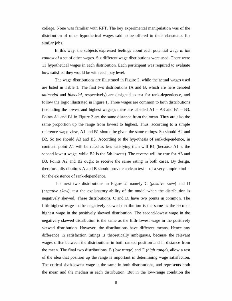
college. None was familiar with RFT. The key experimental manipulation was of the

distribution of other hypothetical wages said to be offered to their classmates for

similar jobs.

In this way, the subjects expressed feelings about each potential wage in the

context of a set of other wages. Six different wage distributions were used. There were

11 hypothetical wages in each distribution. Each participant was required to evaluate

how satisfied they would be with each pay level.

The wage distributions are illustrated in Figure 2, while the actual wages used

are listed in Table 1. The first two distributions (A and B, which are here denoted

unimodal and bimodal, respectively) are designed to test for rank-dependence, and

follow the logic illustrated in Figure 1. Three wages are common to both distributions

(excluding the lowest and highest wages); these are labelled A1 – A3 and B1 – B3.

Points A1 and B1 in Figure 2 are the same distance from the mean. They are also the

same proportion up the range from lowest to highest. Thus, according to a simple

reference-wage view, A1 and B1 should be given the same ratings. So should A2 and

B2. So too should A3 and B3. According to the hypothesis of rank-dependence, in

contrast, point A1 will be rated as less satisfying than will B1 (because A1 is the

second lowest wage, while B2 is the 5th lowest). The reverse will be true for A3 and

B3. Points A2 and B2 ought to receive the same rating in both cases. By design,

therefore, distributions A and B should provide a clean test -- of a very simple kind --

for the existence of rank-dependence.

The next two distributions in Figure 2, namely C (positive skew) and D

(negative skew), test the explanatory ability of the model when the distribution is

negatively skewed. These distributions, C and D, have two points in common. The

fifth-highest wage in the negatively skewed distribution is the same as the second-

highest wage in the positively skewed distribution. The second-lowest wage in the

negatively skewed distribution is the same as the fifth-lowest wage in the positively

skewed distribution. However, the distributions have different means. Hence any

difference in satisfaction ratings is theoretically ambiguous, because the relevant

wages differ between the distributions in both ranked position and in distance from

the mean. The final two distributions, E (low range) and F (high range), allow a test

of the idea that position up the range is important in determining wage satisfaction.

The critical sixth-lowest wage is the same in both distributions, and represents both

the mean and the median in each distribution. But in the low-range condition the

9

critical wage is 60% up the range from lowest to highest wage, while it is 40% up the

range in the high range condition. A difference in the satisfaction from this critical

wage ought then to be unambiguous evidence for a ‘range’ effect on well-being.

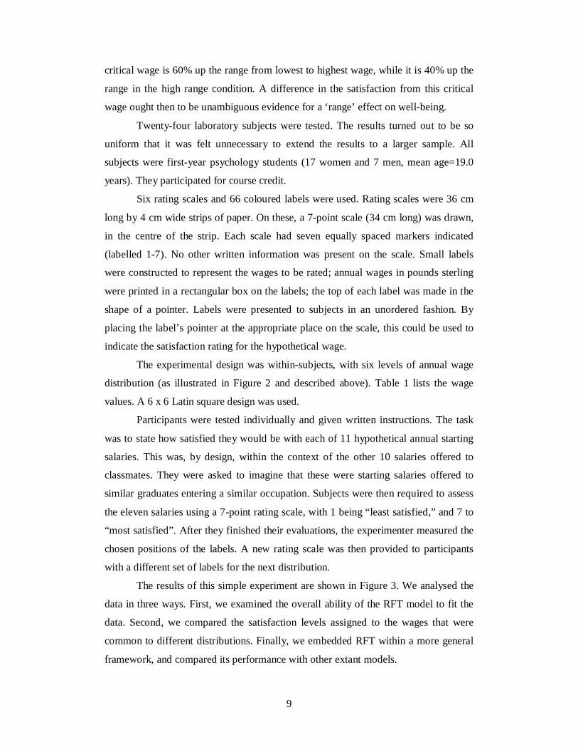
Twenty-four laboratory subjects were tested. The results turned out to be so

uniform that it was felt unnecessary to extend the results to a larger sample. All

subjects were first-year psychology students (17 women and 7 men, mean age=19.0

years). They participated for course credit.

Six rating scales and 66 coloured labels were used. Rating scales were 36 cm

long by 4 cm wide strips of paper. On these, a 7-point scale (34 cm long) was drawn,

in the centre of the strip. Each scale had seven equally spaced markers indicated

(labelled 1-7). No other written information was present on the scale. Small labels

were constructed to represent the wages to be rated; annual wages in pounds sterling

were printed in a rectangular box on the labels; the top of each label was made in the

shape of a pointer. Labels were presented to subjects in an unordered fashion. By

placing the label’s pointer at the appropriate place on the scale, this could be used to

indicate the satisfaction rating for the hypothetical wage.

The experimental design was within-subjects, with six levels of annual wage

distribution (as illustrated in Figure 2 and described above). Table 1 lists the wage

values. A 6 x 6 Latin square design was used.

Participants were tested individually and given written instructions. The task

was to state how satisfied they would be with each of 11 hypothetical annual starting

salaries. This was, by design, within the context of the other 10 salaries offered to

classmates. They were asked to imagine that these were starting salaries offered to

similar graduates entering a similar occupation. Subjects were then required to assess

the eleven salaries using a 7-point rating scale, with 1 being “least satisfied,” and 7 to

“most satisfied”. After they finished their evaluations, the experimenter measured the

chosen positions of the labels. A new rating scale was then provided to participants

with a different set of labels for the next distribution.

The results of this simple experiment are shown in Figure 3. We analysed the

data in three ways. First, we examined the overall ability of the RFT model to fit the

data. Second, we compared the satisfaction levels assigned to the wages that were

common to different distributions. Finally, we embedded RFT within a more general

framework, and compared its performance with other extant models.

10

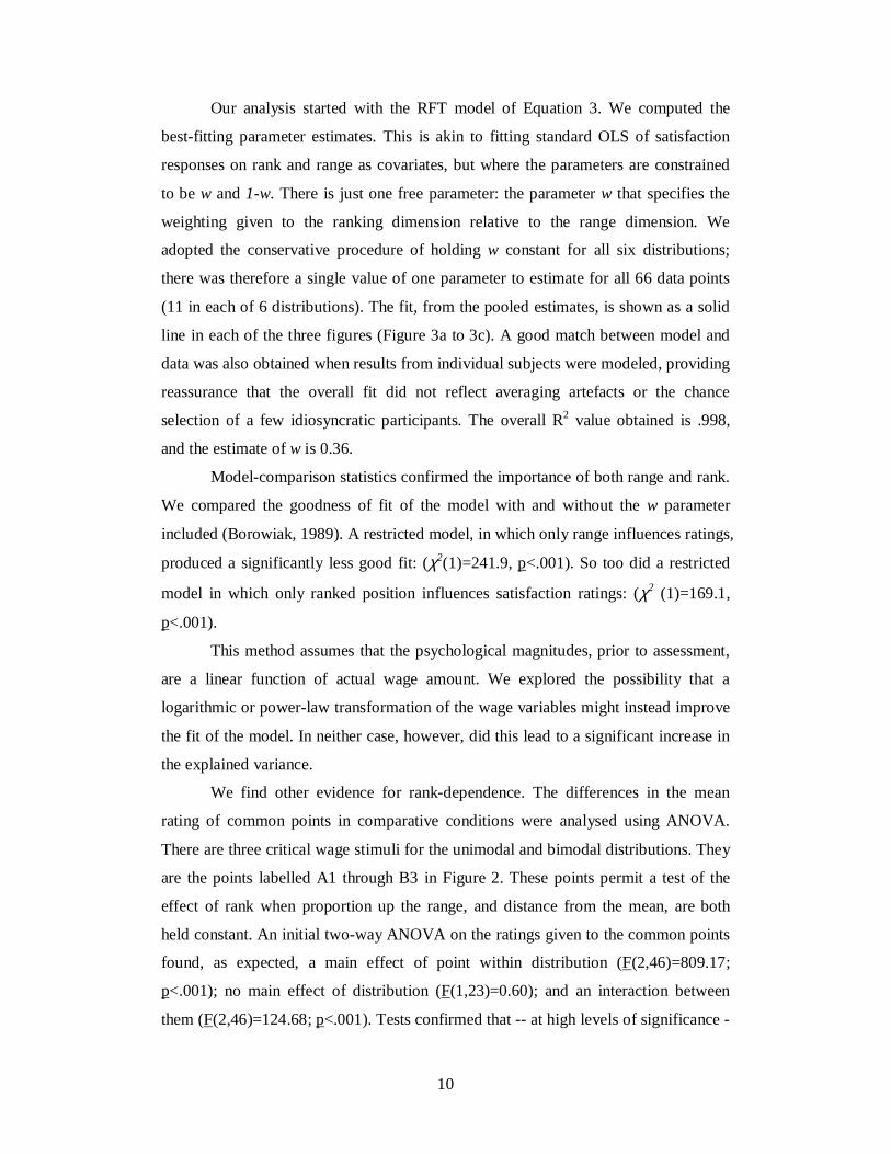
Our analysis started with the RFT model of Equation 3. We computed the

best-fitting parameter estimates. This is akin to fitting standard OLS of satisfaction

responses on rank and range as covariates, but where the parameters are constrained

to be w and 1-w. There is just one free parameter: the parameter w that specifies the

weighting given to the ranking dimension relative to the range dimension. We

adopted the conservative procedure of holding w constant for all six distributions;

there was therefore a single value of one parameter to estimate for all 66 data points

(11 in each of 6 distributions). The fit, from the pooled estimates, is shown as a solid

line in each of the three figures (Figure 3a to 3c). A good match between model and

data was also obtained when results from individual subjects were modeled, providing

reassurance that the overall fit did not reflect averaging artefacts or the chance

selection of a few idiosyncratic participants. The overall R2 value obtained is .998,

and the estimate of w is 0.36.

Model-comparison statistics confirmed the importance of both range and rank.

We compared the goodness of fit of the model with and without the w parameter

included (Borowiak, 1989). A restricted model, in which only range influences ratings,

produced a significantly less good fit: (χ2(1)=241.9, p<.001). So too did a restricted

model in which only ranked position influences satisfaction ratings: (χ2 (1)=169.1,

p<.001).

This method assumes that the psychological magnitudes, prior to assessment,

are a linear function of actual wage amount. We explored the possibility that a

logarithmic or power-law transformation of the wage variables might instead improve

the fit of the model. In neither case, however, did this lead to a significant increase in

the explained variance.

We find other evidence for rank-dependence. The differences in the mean

rating of common points in comparative conditions were analysed using ANOVA.

There are three critical wage stimuli for the unimodal and bimodal distributions. They

are the points labelled A1 through B3 in Figure 2. These points permit a test of the

effect of rank when proportion up the range, and distance from the mean, are both

held constant. An initial two-way ANOVA on the ratings given to the common points

found, as expected, a main effect of point within distribution (F(2,46)=809.17;

p<.001); no main effect of distribution (F(1,23)=0.60); and an interaction between

them (F(2,46)=124.68; p<.001). Tests confirmed that -- at high levels of significance -

11

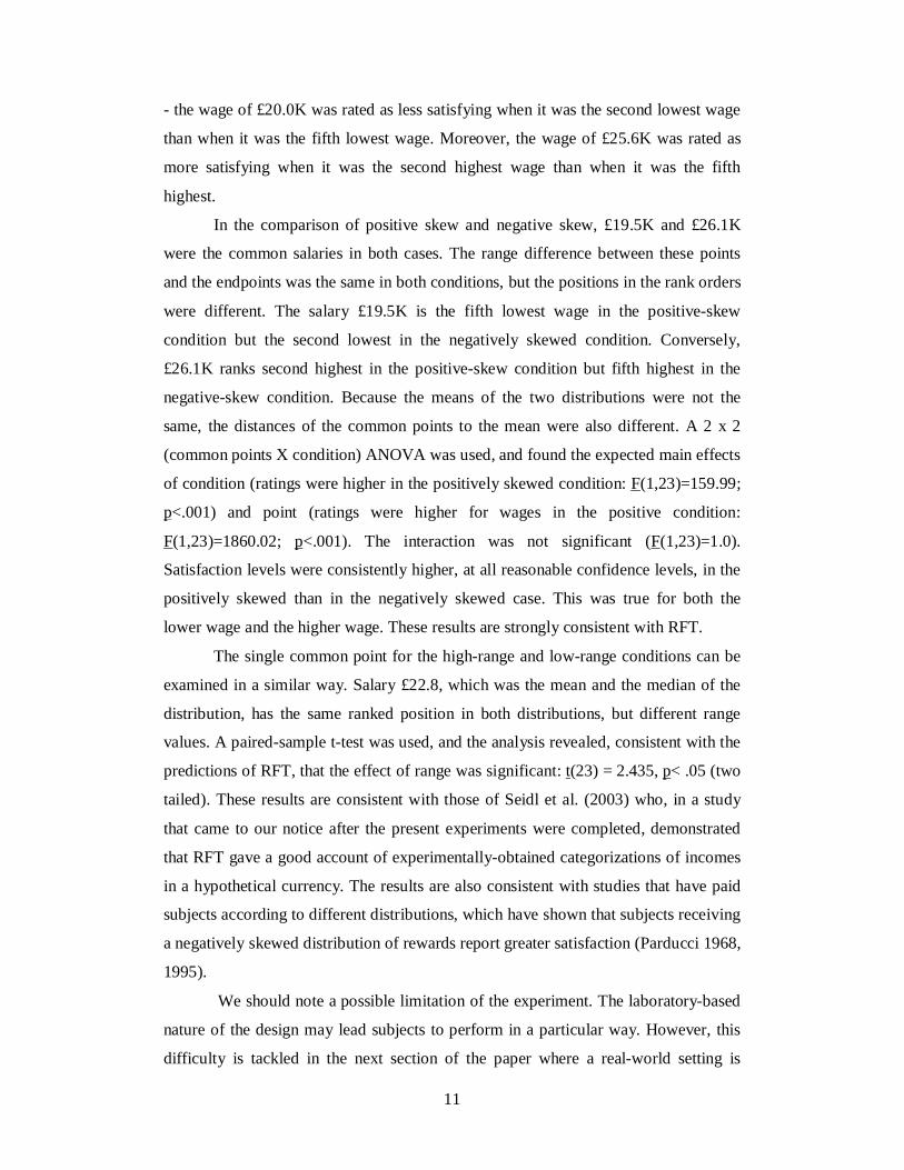
- the wage of £20.0K was rated as less satisfying when it was the second lowest wage

than when it was the fifth lowest wage. Moreover, the wage of £25.6K was rated as

more satisfying when it was the second highest wage than when it was the fifth

highest.

In the comparison of positive skew and negative skew, £19.5K and £26.1K

were the common salaries in both cases. The range difference between these points

and the endpoints was the same in both conditions, but the positions in the rank orders

were different. The salary £19.5K is the fifth lowest wage in the positive-skew

condition but the second lowest in the negatively skewed condition. Conversely,

£26.1K ranks second highest in the positive-skew condition but fifth highest in the

negative-skew condition. Because the means of the two distributions were not the

same, the distances of the common points to the mean were also different. A 2 x 2

(common points X condition) ANOVA was used, and found the expected main effects

of condition (ratings were higher in the positively skewed condition: F(1,23)=159.99;

p<.001) and point (ratings were higher for wages in the positive condition:

F(1,23)=1860.02; p<.001). The interaction was not significant (F(1,23)=1.0).

Satisfaction levels were consistently higher, at all reasonable confidence levels, in the

positively skewed than in the negatively skewed case. This was true for both the

lower wage and the higher wage. These results are strongly consistent with RFT.

The single common point for the high-range and low-range conditions can be

examined in a similar way. Salary £22.8, which was the mean and the median of the

distribution, has the same ranked position in both distributions, but different range

values. A paired-sample t-test was used, and the analysis revealed, consistent with the

predictions of RFT, that the effect of range was significant: t(23) = 2.435, p< .05 (two

tailed). These results are consistent with those of Seidl et al. (2003) who, in a study

that came to our notice after the present experiments were completed, demonstrated

that RFT gave a good account of experimentally-obtained categorizations of incomes

in a hypothetical currency. The results are also consistent with studies that have paid

subjects according to different distributions, which have shown that subjects receiving

a negatively skewed distribution of rewards report greater satisfaction (Parducci 1968,

1995).

We should note a possible limitation of the experiment. The laboratory-based

nature of the design may lead subjects to perform in a particular way. However, this

difficulty is tackled in the next section of the paper where a real-world setting is

12

employed. We also should note that the pay information was simultaneously and

visually available to subjects, perhaps increasing the likelihood that it would be

processed in the same way as other physical stimuli. A further experiment, not

reported here, addressed this issue by presenting wages for sequential evaluation, and

RFT fitted the data.

Compared to RFT theory, how well might other models do? It has been argued

that the notion of fairness needs to be incorporated into conceptions of utility.v If pay

satisfaction depends on perceived unfairness, then models of inequity perception

could be applied to the present case. Given that RFT has already been shown to

provide a good fit to fair-salary increases and tax assignments (Mellers, 1982, 1986),

the present data provide an opportunity to examine the different predictions of RFT

and economic models of inequity as applied to wage satisfaction.

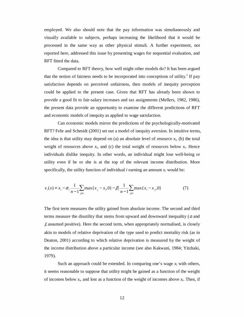
Can economic models mirror the predictions of the psychologically-motivated

RFT? Fehr and Schmidt (2001) set out a model of inequity aversion. In intuitive terms,

the idea is that utility may depend on (a) an absolute level of resource xi, (b) the total

weight of resources above xi, and (c) the total weight of resources below xi. Hence

individuals dislike inequity. In other words, an individual might lose well-being or

utility even if he or she is at the top of the relevant income distribution. More

specifically, the utility function of individual i earning an amount xi would be:

vi (x) = xi −α i

1

n −1max{x j − xi,0}

j ≠ i

∑ − β i

1

n −1max{xi − x j ,0}

j≠ i

∑ (7)

The first term measures the utility gained from absolute income. The second and third

terms measure the disutility that stems from upward and downward inequality (α and

β assumed positive). Here the second term, when appropriately normalised, is closely

akin to models of relative deprivation of the type used to predict mortality risk (as in

Deaton, 2001) according to which relative deprivation is measured by the weight of

the income distribution above a particular income (see also Kakwani, 1984; Yitzhaki,

1979).

Such an approach could be extended. In comparing one’s wage xi with others,

it seems reasonable to suppose that utility might be gained as a function of the weight

of incomes below xi, and lost as a function of the weight of incomes above xi. Then, if

13

the sign of the third term in (7) above is reversed, and α and β are both positive, the

Fehr-Schmidt formulation can be extended to provide a potential model of

comparison-based wage utility.

This version of Fehr-Schmidt model differs from Range Frequency Theory in

one important way. It assumes that higher and lower earners are weighted more

heavily as their distance from xi increases. According to RFT, however, only the

numbers of people with higher and lower incomes matter. Both models contrast with

an alternative approach, developed below, in which incomes similar to xi carry most

weight in determining the utility associated with xi. A further difference between the

Fehr-Schmidt model and RFT is that only the former can accommodate individual

differences in relative concern with upward and downward comparisons. Such

differences exist. For example, Stutzer (2004) found that, when income and other

individual characteristics are controlled for, well-being is lower among people with

higher income aspiration levels.

The principles embodied in RFT, and those incorporated in the Fehr-Schmidt

model, can be seen as special cases of a more general conceptual framework. In

intuitive terms, we can distinguish three different ways in which income-derived

utility might be rank-dependent.

First, as in the Fehr-Schmidt model, higher and lower wages may be weighted

by their difference from xi. Such an approach receives support from the plausibility

and empirical success of similar models of relative deprivation.

Second, as in RFT, the mere ordinal rank of xi may matter.

Third, and contrary to the Fehr-Schmidt approach, incomes relatively close to

xi may contribute more strongly than distant incomes in determining rank-dependent

utility for xi. This idea would be consistent with the considerable weight of evidence

suggesting that social comparisons occur with generally similar agents (e.g. Festinger,

1954) and that pay referents tend to be similar (e.g. Law & Wong, 1998).

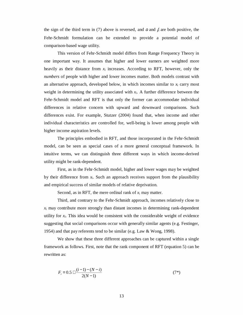
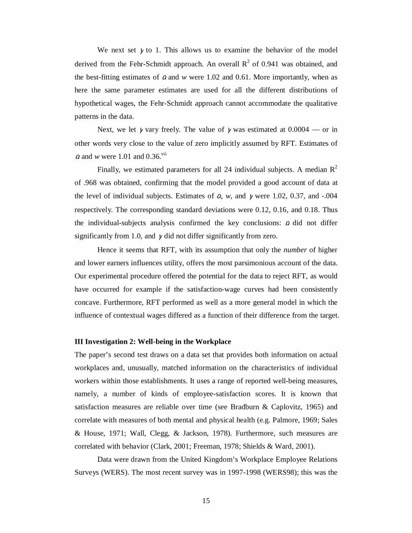
We show that these three different approaches can be captured within a single

framework as follows. First, note that the rank component of RFT (equation 5) can be

rewritten as:

Fi = 0.5+ (i −1) − (N − i)2(N −1)

(7*)

14

where Fi is the frequency value of wage xi and N is the number of incomes in the

comparison set. Thus for a fixed comparison set, Fi decreases linearly with the

number of higher incomes (N-i) and increases linearly with the number of lower

incomes (i-1).

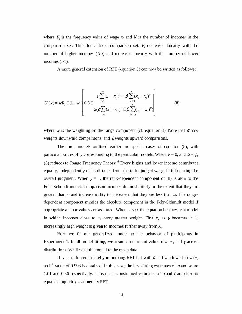
A more general extension of RFT (equation 3) can now be written as follows:

U i (x) = wRi + (1− w ) 0.5+α (

j =1

i−1

∑ xi − x j )γ − β (

j= i +1

N

∑ x j − xi )γ

2(α (j =1

i−1

∑ xi − x j )γ + β (

j = i+1

N

∑ x j − xi )γ )

(8)

where w is the weighting on the range component (cf. equation 3). Note that α now

weights downward comparisons, and β weights upward comparisons.

The three models outlined earlier are special cases of equation (8), with

particular values of γ corresponding to the particular models. When γ = 0, and α = β,

(8) reduces to Range Frequency Theory.vi Every higher and lower income contributes

equally, independently of its distance from the to-be-judged wage, in influencing the

overall judgment. When γ = 1, the rank-dependent component of (8) is akin to the

Fehr-Schmidt model. Comparison incomes diminish utility to the extent that they are

greater than xi and increase utility to the extent that they are less than xi. The range-

dependent component mimics the absolute component in the Fehr-Schmidt model if

appropriate anchor values are assumed. When γ < 0, the equation behaves as a model

in which incomes close to xi carry greater weight. Finally, as γ becomes > 1,

increasingly high weight is given to incomes further away from xi.

Here we fit our generalized model to the behavior of participants in

Experiment 1. In all model-fitting, we assume a constant value of α, w, and γ across

distributions. We first fit the model to the mean data.

If γ is set to zero, thereby mimicking RFT but with α and w allowed to vary,

an R2 value of 0.998 is obtained. In this case, the best-fitting estimates of α and w are

1.01 and 0.36 respectively. Thus the unconstrained estimates of α and β are close to

equal as implicitly assumed by RFT.

15

We next set γ to 1. This allows us to examine the behavior of the model

derived from the Fehr-Schmidt approach. An overall R2 of 0.941 was obtained, and

the best-fitting estimates of α and w were 1.02 and 0.61. More importantly, when as

here the same parameter estimates are used for all the different distributions of

hypothetical wages, the Fehr-Schmidt approach cannot accommodate the qualitative

patterns in the data.

Next, we let γ vary freely. The value of γ was estimated at 0.0004 — or in

other words very close to the value of zero implicitly assumed by RFT. Estimates of

α and w were 1.01 and 0.36.vii

Finally, we estimated parameters for all 24 individual subjects. A median R2

of .968 was obtained, confirming that the model provided a good account of data at

the level of individual subjects. Estimates of α, w, and γ were 1.02, 0.37, and -.004

respectively. The corresponding standard deviations were 0.12, 0.16, and 0.18. Thus

the individual-subjects analysis confirmed the key conclusions: α did not differ

significantly from 1.0, and γ did not differ significantly from zero.

Hence it seems that RFT, with its assumption that only the number of higher

and lower earners influences utility, offers the most parsimonious account of the data.

Our experimental procedure offered the potential for the data to reject RFT, as would

have occurred for example if the satisfaction-wage curves had been consistently

concave. Furthermore, RFT performed as well as a more general model in which the

influence of contextual wages differed as a function of their difference from the target.

III Investigation 2: Well-being in the Workplace

The paper’s second test draws on a data set that provides both information on actual

workplaces and, unusually, matched information on the characteristics of individual

workers within those establishments. It uses a range of reported well-being measures,

namely, a number of kinds of employee-satisfaction scores. It is known that

satisfaction measures are reliable over time (see Bradburn & Caplovitz, 1965) and

correlate with measures of both mental and physical health (e.g. Palmore, 1969; Sales

& House, 1971; Wall, Clegg, & Jackson, 1978). Furthermore, such measures are

correlated with behavior (Clark, 2001; Freeman, 1978; Shields & Ward, 2001).

Data were drawn from the United Kingdom’s Workplace Employee Relations

Surveys (WERS). The most recent survey was in 1997-1998 (WERS98); this was the

16

first to include employee questionnaires and it is these that provide the data for the

research reported here. The data set allows us to match up information on individual

workers with information on the plants that employ them.

All places of employment in Britain -- including schools, shops, offices and

factories -- with ten or more employees were eligible to be sampled. For this study,

the usable sample is 1782 workplaces. Approximately 28,000 employees contributed

completed questionnaires (a response rate of 64%). Up to 25 employee questionnaires

were distributed to randomly-selected employees within each organisation. The

design of WERS98 is summarised in Cully (1998); initial findings from the study are

described in Cully et al. (1998).

Employees were given self-completion questionnaires. They could return them

either via the workplace or directly to the survey agency. Questions focussed on a

range of issues including Employee Attitudes to Work, Payment Systems, Health &

Safety, Worker Representation, and other related areas.

The variables of particular interest to us are four measures of worker

satisfaction, as listed below. Question A10 from the Survey was phrased as follows:

“How satisfied are you with the following aspects of your job?”

Four aspects were listed:

“The amount of influence you have over your job”;

“The amount of pay you receive”;

“The sense of achievement you get from your work”, and

“The respect you get from supervisors/line managers”.

A primary interest here will be on satisfaction with the amount of pay. It would not be

surprising if measures such as satisfaction with influence are determined by an

individual’s wage rank. Because we do not have an overall job-satisfaction measure in

the data set, we present satisfaction equations for all measures available.

Answers were on a five-point scale ranging from 1 (Very Satisfied) to 5 (Very

Dissatisfied). A sixth “Don’t Know” option was also available. For ease of

interpretation, the scaling here is reversed. Thus the number 5 represents the highest

level of satisfaction. The satisfaction distributions themselves have thicker tails at the

upper than the lower end. For example, on satisfaction with achievement, which is

representative, approximately 15% of respondents give the answer ‘very satisfied’,

50% say ‘satisfied’, 21% say ‘neither satisfied nor dissatisfied’, 11% say ‘dissatisfied’,

and 4% say ‘very dissatisfied’.

17

The independent influences upon satisfaction include wage-related variables

and background variables (which are included as controls within later regression

equations). These background variables, listed in Table 2, are the age of the worker,

the size of the plant, whether the worker is on a temporary contract, the educational

level of the worker, gender, race, a union dummy, occupation, industry, region, hours

worked by the employee, and the marital status of the employee.

It is necessary for the analysis to construct a variety of wage measures. The

variables we test as determinants of well-being include:

1. wabs. Weekly pay of individual i

2. wmean. Average pay in workplace j

3. wrank. Rank of individual i in workplace j as proportion of number of workers,

where greater rank indicates the worker is, in an ordinal sense, higher up the

pay scale. This rank variable is calculated as (rankij - 1)/(number of

observations workplacej - 1)

4. wrange. The distance the individual worker is up the range of payi in workplace

j. This is calculated as a proportion as: (payi - payjmin)/(payj

max - payjmin).

For consistency with earlier literature, we work with mean wage rather than median

wage. Both Rank and Range are defined so as to lie in the unit interval. Moreover,

wabs and wmean are logarithmically transformed except where otherwise stated. Finally,

rank and range (and mean wage) are calculated empirically over the samples drawn

from each establishment.

These different measures of pay are, of course, somewhat correlated.

Nevertheless, the large number of observations makes it possible, in practice, to

estimate the separate variables’ effects. The paper tests whether, with other factors

held constant, wrank and wrange help to determine workers’ satisfaction levels.

We generally worked with data collected from all workplaces that had at least

15 employee-pay observations. The resulting sample contained 16,266 individuals

from 886 separate workplaces.

The raw correlations between the main variables are shown in Table 3. Not

surprisingly, workers’ reported well-being levels are in all but 3 of the 16 cases

positively correlated with their (various measures of) remuneration. Four different

satisfaction measures are available. These could be combined into a single average,

but we decided it would be more transparent not to do so. Within Table 3, there are

four wage measures. These are the log of the worker’s pay, the log of mean pay in the

18

plant, the worker’s rank in the wage ordering, and the range of pay within the plant.

Out of necessity, they are calculated within the available sample, and are thus best

thought of as estimates. In other words, here the rank and range for worker i are for

the sample of workers available within WERS. Compared to the true model of the

whole workplace, this means that Rank and Range are measured with error, which

will tend to make it harder to find statistically significant effects. The pay measures

are intercorrelated, with wabs (log transformed) having a correlation greater than 0.6

with all of wrank, wrange, and wmean (log transformed). Even in the raw data depicted in

Table 3, wrank is more highly correlated with satisfaction than any other pay measure.

For instance, in the case of a sense of achievement, the correlation coefficient is 0.086

with pay rank, compared to only 0.021 with actual pay.

Ordered probit analysis was undertaken. The background measures listed in

Table 2 were always included; we do not report the coefficients for these variables,

although the results are available on request. All columns in the regression tables

reported below were estimated by the ordered probit technique. Standard errors are in

parentheses and are robust to arbitrary heteroscedasticity and clustering bias. The

Pseudo R2 values were calculated using the McKelvey-Zavoina method. Pay

measures were log transformed, but the findings were checked with untransformed

measures and similar results were obtained. Although, in general, ordered probit

coefficients do not have the simple interpretation of OLS coefficients, we have

checked that in later equations the coefficients can typically be read off in a fairly

intuitive way.

After controlling for other factors, does satisfaction depend upon the level of

pay? Table 4a shows the results for the largest possible sample. Table 4b gives the

results for a restricted sample that excludes small plants. There are four satisfaction

equations: for Influence, Pay, Achievement and Respect. Each well-being regression

equation is to be read vertically. In both the full and the restricted sample, the

logarithm of absolute pay wabs has a statistically significant effect within the four

satisfaction equations. The coefficients are similar in both samples. This preliminary

analysis provides reassurance that the restricted sample is representative; subsequent

analysis focuses on the restricted sample alone as it was deemed more reliable for

analysis of wrange and wrank.

Next, we test for comparison effects. Our data are rich in that they allow us to

compute the average pay within the workplace. Hence we can do a more direct test

19

than Clark and Oswald (1996), who define an individual’s comparison group as those

workers in the data set who have similar characteristics to the individual. The result of

adding wmean into the equation is shown in Table 5. In each case, the own-wage

variable, which is denoted Ln(pay), remains positive, and its coefficient is statistically

significantly different from zero in all of the four columns. Money continues,

therefore, to buy extra well-being. For Table 5’s satisfaction equations for Influence,

Achievement and Respect, the comparison wage wmean enters with a negative

coefficient, with a standard error generally of approximately one third of the

coefficient. Interestingly, wmean accounts for little or no significant additional variance

within the 2nd column’s equation for pay satisfaction. Moreover, it has a positive sign.

It is possible that this is the ‘ambition’ effect of Senik (2006), namely, that workers

are pleased to work somewhere where their pay may rise through future promotions.

But that can only be a conjecture.

To summarize, we find quite strong evidence for a relative-wage effect upon

satisfaction. This is true for three of the four measures of reported well-being, and

after controlling for a set of worker and workplace characteristics. Table 5 therefore

adds to an accumulating econometric literature on comparison effects upon well-being.

Next, to nest Range Frequency Theory within the framework, the wrank and

wrange measures are added into each well-being equation. The results are shown in

Table 6a. This is the specification for the more general model set out earlier in

equation 6.

The results seem quite striking. To an economist, particularly given the likely

amount of measurement error, it might be viewed as surprising that variables such as

rank – where I lie in an ordinal sense in a sample of 25 workers from my

establishment – partially predicts reported satisfaction with pay. Nevertheless, that is

what the data seem to show.

In Table 6a, the variable measuring the individual worker’s position in the pay

ordering wrank works strongly in the equations. It has an independent positive effect in

a way consistent with the hypothesis of rank-dependence. This is perhaps the main

finding of the paper: in both the laboratory and in real-world data there is evidence

that ordinal rank matters, and indeed may matter more than the level of pay itself.

The coefficient for wmean in the pay satisfaction equation is, rather

unexpectedly, positive.viii The coefficients on wmean in the other three columns in

Table 6a are not significantly different from zero at the 5% level. One possible

20

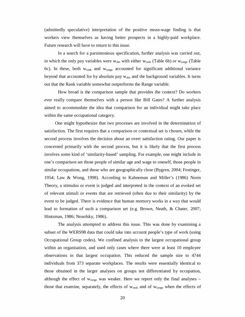
(admittedly speculative) interpretation of the positive mean-wage finding is that

workers view themselves as having better prospects in a highly-paid workplace.

Future research will have to return to this issue.

In a search for a parsimonious specification, further analysis was carried out,

in which the only pay variables were wabs with either wrank (Table 6b) or wrange (Table

6c). In these, both wrank and wrange accounted for significant additional variance

beyond that accounted for by absolute pay wabs and the background variables. It turns

out that the Rank variable somewhat outperforms the Range variable.

How broad is the comparison sample that provides the context? Do workers

ever really compare themselves with a person like Bill Gates? A further analysis

aimed to accommodate the idea that comparison for an individual might take place

within the same occupational category.

One might hypothesize that two processes are involved in the determination of

satisfaction. The first requires that a comparison or contextual set is chosen, while the

second process involves the decision about an overt satisfaction rating. Our paper is

concerned primarily with the second process, but it is likely that the first process

involves some kind of ‘similarity-based’ sampling. For example, one might include in

one’s comparison set those people of similar age and wage to oneself, those people in

similar occupations, and those who are geographically close (Bygren, 2004; Festinger,

1954; Law & Wong, 1998). According to Kahneman and Miller’s (1986) Norm

Theory, a stimulus or event is judged and interpreted in the context of an evoked set

of relevant stimuli or events that are retrieved (often due to their similarity) by the

event to be judged. There is evidence that human memory works in a way that would

lead to formation of such a comparison set (e.g. Brown, Neath, & Chater, 2007;

Hintzman, 1986; Nosofsky, 1986).

The analysis attempted to address this issue. This was done by examining a

subset of the WERS98 data that could take into account people’s type of work (using

Occupational Group codes). We confined analysis to the largest occupational group

within an organisation, and used only cases where there were at least 10 employee

observations in that largest occupation. This reduced the sample size to 4744

individuals from 373 separate workplaces. The results were essentially identical to

those obtained in the larger analyses on groups not differentiated by occupation,

although the effect of wrange was weaker. Here we report only the final analyses –

those that examine, separately, the effects of wrank and of wrange when the effects of

21

wabs, are partialled out. The results are in Tables 7a and 7b. It is evident that wage

satisfaction, as well as most other satisfaction measures, is independently predicted by

wrank. As before, the Rank effect is positive and seems highly robust. Because of the

size of the sample, it was not possible to estimate simultaneously the effects of range

and rank in workplaces and occupations.

Although the emphasis here has been on whether rank and range have

statistically significant effects, their size is also of interest. As one fairly

representative example, consider the variable ‘satisfaction with achievement’. In this

case, a movement in Rank from zero to unity raises quite noticeably the likelihood of

being satisfied. The probability of giving either the top or second-top satisfaction

answer here increases, holding the other independent variables constant, from

approximately 61% to 70%. To put this in perspective, in most specifications the level

of absolute pay would have to more than triple to get the same effect.

Some potential criticisms and counter-arguments should be mentioned.

• First, there is no guarantee in these workplaces that workers actually

know other people’s wage rates. All we can say is that people act as

though they are able to form a reasonable estimate of where, as

individuals, they lie in the pay ordering and the range. It would be

interesting to examine plants and offices with confidential pay scales,

and to ascertain whether people want others to be able to see that they

are high in income-rank.

• Second, it seems important to understand exactly how a person

chooses a reference group. Our paper has little to contribute to this

issue. We are forced in our econometric specification simply to assume

that the workplace is the comparison set.

• Third, given the sometimes positive nature of comparisons in the pay

satisfaction equations, it would be interesting to be able to say more

about the lifetime dynamics of pay. Low wages today may be

compensated by high wages after promotion tomorrow. More research

here will be needed.

• Fourth, we are unable to control directly for job titles, and this kind of

‘rank’ is likely also to play a role in well-being, even though it is

unobservable in our data set.

22

• Fifth, without enormous samples, measurement error is inevitably a

problem in the construction of our Rank and Range variables. In this

study, probably the best that can be done is to check, as we have done,

that the findings go through for sub-samples of small as well as large

workplaces.

• Sixth, in principle, it might be that wage variables such as Rank are

merely proxying for an omitted non-linearity in the form that absolute

pay takes in the well-being equations. Our checks with higher-order

pay polynomials, however, suggest that this is not the explanation.

• Seventh, it might perhaps be argued that an allowance for additional

‘moments’ of the pay distribution is bound to improve upon simpler

specifications, so that, by Occam’s razor, standard models should be

preferred. Yet that objection seems to miss the key point. Our data

suggest that, when a direct comparison is done, a rank variable

strongly outperforms a simple relative-wage variable.

• Eighth, could it be that Rank is merely a proxy for omitted variables

like job autonomy, and it is those omitted factors that raise well-being?

It is never feasible in empirical research to dispose entirely of this kind

of possibility. Nevertheless, the first section of the paper shows that

RFT fits the data in an experimental setting where there is no influence

from job characteristics like autonomy.

IV Investigation 3: Quits in Workplace Data

Up to this point, the paper has concentrated on reported levels of well-being, and has

viewed those numbers as providing proxy utility data. Such an approach seems to be

of some worth in its own right. It also fits with much recent literature, such as Luttmer

(2005). However, to show that RFT also has implications for observable actions, we

now estimate labor-turnover equations.

Information on the individual workers who choose to leave is not available

within our data set. Hence it is not possible to do a micro-data test on people’s labor

turnover decisions.

Nevertheless, workplaces do provide data on the total number of quits in the

previous year. This makes it possible, by using information on workplace size, to

23

calculate the quit rate per plant. Range Frequency Theory has the implication that

workers will tend to quit more when -- following a version of equation 6 -- the

distribution of wages at the plant produces a low level of utility from the job.

A key prediction of RFT is that negative skewness of a pay distribution leads

to workers who are more content. This prediction arises because the mean level of

happiness is greater if the majority of workers are near the top of the salary range paid

by the employer. Will a measure of the skewness of wages independently predict the

level of quits in a regression equation? We construct a test of this sort.

After discarding the plants where fewer than 15 workers provided details to

the survey, we are left with a usable sample of approximately 900 workplaces. Table

8 describes the raw data. The quit rate in the sample is approximately 14% of

employees per annum. Mean pay in the sample is approximately 258 pounds per week.

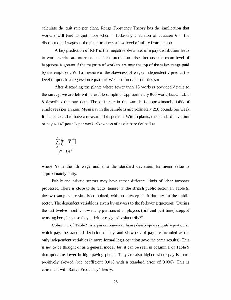
It is also useful to have a measure of dispersion. Within plants, the standard deviation

of pay is 147 pounds per week. Skewness of pay is here defined as:

Yi −Y( )3

i=1

N

∑

(N −1)s3

where Yi is the ith wage and s is the standard deviation. Its mean value is

approximately unity.

Public and private sectors may have rather different kinds of labor turnover

processes. There is close to de facto ‘tenure’ in the British public sector. In Table 9,

the two samples are simply combined, with an intercept-shift dummy for the public

sector. The dependent variable is given by answers to the following question: "During

the last twelve months how many permanent employees (full and part time) stopped

working here, because they ... left or resigned voluntarily?".

Column 1 of Table 9 is a parsimonious ordinary-least-squares quits equation in

which pay, the standard deviation of pay, and skewness of pay are included as the

only independent variables (a more formal logit equation gave the same results). This

is not to be thought of as a general model, but it can be seen in column 1 of Table 9

that quits are lower in high-paying plants. They are also higher where pay is more

positively skewed (see coefficient 0.018 with a standard error of 0.006). This is

consistent with Range Frequency Theory.

24

Column 2 of Table 9 adds in region dummies, industry dummies (to try to

account for, among other things, ‘sunset technologies’ where there is high level of

quits), a public-sector dummy, and measure of workplace size. The coefficient on

Skewness falls somewhat, from 0.18 to 0.10, and marginally loses significance at the

5% level. However, a fuller, and arguably the most natural, specification is set out in

the third and final column of Table 9. Here the quits equation allows also for a

number of controls of the sort suggested by labor economics -- including the

proportion of people with occupational pensions, whether the workplace is formally

unionized, the proportion of female workers, and two variables that capture the age

composition of the workplace. Now the coefficient on the skewness variable is

estimated at 0.12. This coefficient is significantly different from zero at the 5% level.

Moreover, on these estimates, the effect that the shape of the pay distribution has

upon quits is not trivially small. A one-standard-deviation increase in Skewness here

raises the quit rate by a little more than one percentage point per annum. This is close

in size to, for example, the effect of a one-standard-deviation drop in the proportion of

workers over 50 years of age.

Standard deviation of pay does not enter statistically significantly in the

equations, but is retained as a control to ensure that skewness is not standing in for

some simpler measure of the second moment of a distribution. Nothing of substance

alters by removing the standard-deviation variable from the regressors. We also

checked whether various controls for workers’ education levels entered the quits

equation, but their coefficients were never statistically significantly different from

zero.

Table 10 gives the equivalent quits equation for private-sector workers alone.

Our sample size is now slightly less than 600 workplaces, and the coefficients are not

always precisely estimated. But the broad pattern is the same. Skewness enters in a

statistically significant way in columns 2 and 3 of Table 10. Here the coefficient is

approximately 0.02, and again the standard deviation of skewness is approximately

unity, so the size of this effect is actually a little larger than in the public-plus-private-

sector full sample. Once again, the findings are consistent with a Parducci-style model.

Finally, we experimented with another variable -- one for the average value of

‘range’ within each establishment. This mean range variable worked with the correct

sign but its t-statistic was not reliably larger than 2. Our instinct is that skewness here

is a better measure theoretically, because it goes some way to capture the fact that it is

25

disproportionately the workers low down a pay distribution who are likely to quit. As

explained earlier, skewness is also directly emphasised by Parducci.

V Conclusion

This paper is an attempt to understand wage comparisons and the determinants of

well-being in the workplace. By combining laboratory and econometric evidence, the

paper draws three conclusions.

First, human beings do not care solely about their absolute level of pay.

Workers are concerned, the paper shows, with their income relative to the

remuneration levels around them in their workplace. In this sense, the work is in the

spirit of a tradition that includes in the modern era Frank (1985), Clark and Oswald

(1996) and Luttmer (2005), and before them Duesenberry (1949). Comparisons matter.

Second, although we uncover some econometric evidence for a simple

relative-income formulation in which utility is given by a function u = u(pay, relative

pay), the main contribution of the paper is an attempt to go beyond this. Using a

sample of 16,000 workers from 900 workplaces, the paper argues that ordinal rank

has a statistically significant effect upon well-being, and that to understand what

makes human beings content it is therefore necessary to look at the whole distribution

of incomes. The paper appears to be one of the first in the industrial relations and

economics literatures to provide workplace evidence for the importance of income

rank.

Third, using data on quits, the paper finds evidence that greater positive-

skewness in the pay distribution is, as Allen Parducci’s work predicts, associated with

higher labor turnover.

It is natural to think of possible evolutionary motives behind a concern for

ordinal position among human beings, but it is currently not possible to say exactly

why rank, range and skewness have the effects we observe in workplace data.

Nevertheless, the results in this paper suggest that Range Frequency Theory -- a

conceptual account still unknown to most economists and industrial relations

researchers -- may be valuable to the disciplines of labor economics and industrial

relations.

26

References

Akerlof, George A., and Janet L. Yellen. 1990. “The Fair Wage-effort Hypothesis and

Unemployment.” Quarterly Journal of Economics 105 (May):255-283.

Birnbaum, Michael H. 1992. “Violations of Monotonicity and Contextual Effects in

Choice-Based Certainty Equivalents.” Psychological Science 3

(September):310-314.

Blanchflower, David, and Andrew J. Oswald. 2004. “Well-being over Time in Britain

and the USA.” Journal of Public Economics 88 (July):1359-1386.

Bolton, Gary E. 1991. “A Comparative Model of Bargaining: Theory and Evidence.”

American Economic Review 81 (December):1096-1136.

Borowiak, Dale S. 1989. Model Discrimination for Nonlinear Regression Models.

New York: Marcel Dekker.

Boskin, Michael, and Eytan Sheshinski. 1978. “Optimal Redistributive Taxation when

Individual Welfare Depends upon Relative Income.” Quarterly Journal of

Economics 92 (November):589-601.

Bradburn, Norman, and David Caplovitz. 1965. Reports on Happiness. Chicago, IL:

Aldine.

Brown, Gordon D.A., Neath, Ian., and Nick Chater. 2007. “A Temporal Ratio Model

of Memory.” Psychological Review 114 (July):539-576.

Brown, Gordon D.A., and Jing Qian. 2004. “The Origin of Probability Weighting: A

Psychophysical Approach.” Manuscript Submitted for Publication.

Bygren, Magnus. 2004. “Pay Reference Standards and Pay Satisfaction: What Do

Workers Evaluate Their Pay Against?” Social Science Research 33 (June):206-

224.

Cappelli, Peter, and Peter D. Sherer. 1988. “Satisfaction, Market Wages, and Labor

Relations: An Airline Study.” Industrial Relations 27 (January):56-73.

Clark, Andrew E. 2000. “Is Utility Absolute or Relative? Some Recent Findings.”

Revue Economique 51 (May):459-471.

Clark, Andrew E. 2001. “What Really Matters In A Job? Hedonic Measurement

Using Quit Data.” Labour Economics 8 (May): 223-242.

Clark, Andrew E. 2003. "Unemployment as a Social Norm: Psychological Evidence

from Panel Data.” Journal of Labor Economics 21 (April):323-351.

Clark, Andrew E., and Andrew J. Oswald. 1996. “Satisfaction and Comparison

Income." Journal of Public Economics 61 (September):359-381.

27

Cox, James, and Ronald Oaxaca. 1989. “Laboratory Experiments With a Finite

Horizon Job Search Model.” Journal of Risk and Uncertainty 2

(September):301-329.

Cully, Mark. 1998. A Survey in Transition: The Design of the 1998 Workplace

Employee Relations Survey. London: Department of Trade and Industry.

Cully, Mark, Woodland, Stephen, O’Reilly, Andrew, Dix, Gill, Millward, Neil,

Bryson, Alex, and John Forth. 1998. The 1998 workplace employee relations

survey: First findings. London: Department of Trade and Industry.

Deaton, Angus. 2001. “Relative Deprivation, Inequality, and Mortality”. Unpublished

manuscript.

Di Tella, Rafael., and Robert MacCulloch. 2005. “Social Partisan Happiness.”

Review of Economic Studies 72 (April):367-393.

Easterlin, Richard A. 1974. “Does Economic Growth Improve the Human Lot? Some

Empirical Evidence.” In Nations and Households in Economic Growth: Essays

in Honor of Moses Abramowitz, edited by Paul A. David and Melvin W. Reder.

New York: Academic Press.

Easterlin, Richard A. 1995. “Will Raising the Incomes of All Increase the Happiness

of All?” Journal of Economic Behavior and Organization 27 (June):35-48.

Fehr, Ernst, and Klaus M. Schmidt. 1999. “A Theory of Fairness, Competition, and

Cooperation.” Quarterly Journal of Economics 114 (August):817-868.

Fehr, Ernst, and Klaus M. Schmidt. 2001. “Theories of Fairness and Reciprocity-

Evidence And Economic Applications.” CEPR Discussion Paper Series,

February.

Festinger, Leon. 1954. “A Theory of Social Comparison Processes.” Human

Relations 7 (May):117-140.

Frank, Robert H. 1985. Choosing the Right Pond: Human Behaviour and the Quest

for Status. London: Oxford University Press.

Freeman, Richard B. 1978. “Job Satisfaction as an Economic Variable.” American

Economic Review 68 (May):135-141.

Frey, Bruno S., and Alois Stutzer. 2002. Happiness and Economics. Princeton and

Oxford: Princeton University Press.

Gilboa, Itzhak., and David Schmeidler. 2001. “A Cognitive Model of Individual

Well-Being.” Social Choice Welfare 18 (2):269-288

28

Goodman, Paul S. 1974. “An Examination of Referents Used in the Evaluation of

Pay.” Organizational Behavior and Human Performance 12 (October):170-195.

Groot, Wim, and Henriette M. Van Den Brink. 1999. “Overpayment and Earnings

Satisfaction: An Application of an Ordered Response Tobit Model.” Applied

Economics Letters 6 (April):235-238.

Hagerty, Michael R. 2000. “Social Comparisons of Income in One’s Community:

Evidence from National Surveys of Income and Happiness.” Journal of

Personality and Social Psychology 78 (April):764-771.

Helson, Harry. 1964. Adaptation-Level Theory. Oxford, England: Harper and Row.

Hamermesh, Daniel S. 1975. Interdependence in the labor market. Economica 42

(November):420-429.

Highhouse, Scoot, Brooks-Laber, Margaret E., Lin, Lilly, and Christiane Spitzmueller.

2003. “What Makes a Salary Seem Reasonable? Frequency Context Effects on

Starting-Salary Expectations.” Journal of Occupational and Organizational

Psychology 76 (March):69-81.

Hills, Frederick S. 1980. “The Relevant Other In Pay Comparisons.” Industrial

Relations 19 (Fall):345-350.

Hintzman, Douglas L. 1986. “Schema Abstraction in a Multiple-Trace Memory

Model.” Psychological Review 93 (October):411-428.

Hopkins, Ed, and Tatiana Kornienko. 2004. “Running to Keep in the Same Place:

Consumer Choice as a Game of Status.” American Economic Review 94

(September):1085-1107.

Janiszewski, Chris and Donald R. Lichtenstein. 1999. “A Range Theory Account of

Price Perception.” Journal of Consumer Research 25 (March):353-368.

Kahneman, Daniel. 1992. “Reference Points, Anchors, Norms, and Mixed Feelings.”

Organizational Behavior and Human Decision Processes 51 (March):296-312.

Kahneman, Daniel, and Dale T. Miller. 1986. "Norm Theory: Comparing Reality to

its Alternatives." Psychological Review 93 (April):136-153.

Kahneman, Daniel, and Amos Tversky. 1979. "Prospect Theory: An Analysis of

Decision under Risk." Econometrica 47 (March):263-291.

Kakwani, Nanak. 1984. "The Relative Deprivation Curve and its Applications."

Journal of Business & Economic Statistics 2 (October):384-394.

Kapteyn, Arie., and Tom Wansbeek. 1985. "The Individual Welfare Function: A

Review." Journal of Economic Psychology 6 (December):333-363.

29

Kornienko, Tatiana. 2004. "A Cognitive Basis for Cardinal Utility." Unpublished

manuscript.

Kosicki, George. 1987. "A Test of the Relative Income hypothesis." Southern

Economic Journal 54 (October):422-434.

Law, Kenneth S., and Chi-Sum Wong. 1998. "Relative Importance of Referents on

Pay Satisfaction: A Review and Test of a New Policy-capturing Approach."

Journal of Occupational and Organizational Psychology 71 (March):47-60.

Layard, Richard. 1980. "Human Satisfactions and Public Policy." Economic Journal

90 (December):737-750.

Layard, Richard. 2005. Happiness: Lessons from a New Science. London: Allen-Lane.

Levine, David I. 1993. "Fairness, Markets, and Ability to Pay: Evidence from

Compensation Executives." American Economic Review 83 (December):1241-

1259.

Lommerud, Kjell E. 1989. "Educational Subsidies when Relative Income Matters."

Oxford Economic Papers 41 (July):640-652.

Lopes, Lola L. 1987. “Between Hope and Fear: The Psychology of Risk.”

In Advances in Experimental Social Psychology (Vol. 20), edited by Leonard

Berkowitz, pp.255-295. San Diego, CA: Academic Press.

Luttmer, Erzo. 2005. "Neighbors as Negatives: Relative Earnings and Well-being."

Quarterly Journal of Economics 120 (August):963-1002.

Marmot, Michael G. 1994. "Social Differences in Health within and between

Populations." Daedalus 123 (Fall):197-216.

Marmot, Michael G., & Bobak, Martin. 2000. "International Comparators and Poverty

and Health in Europe." British Medical Journal 321 (November):1124-1128.

McBride, Michael. 2001. "Relative-income Effects on Subjective Well-being in the

Cross-section." Journal of Economic Behavior and Organization 45 (July):251-

278.

Mellers, Barbara A. 1982. "Equity Judgment: A Revision of Aristotelian Views."

Journal of Experimental Psychology: General 111 (June):242-270.

Mellers, Barbara A. 1986. "“Fair” allocations of salaries and taxes." Journal of

Experimental Psychology: Human Perception and Performance 12 (1):80-91.

Mellers, Barbara A., Ordoñez, Lisa D., and Michael H.Birnbaum. 1992. "A Change-

of-process Theory for Contextual Effects and Preference Reversals in Risky

30

Decision Making." Organizational Behavior and Human Decision Processes 52

(August):331-369.

Munro, Alistair, and Robert Sugden. 2003. "On the Theory of Reference-dependent

Preferences." Journal of Economic Behavior and Organization 50 (April):407-

428.

Niedrich, Ronald W., Sharma, Subhash, and Douglas H. Wedell. 2001. “Reference

Price and Price Perceptions: A Comparison of Alternative Models.” Journal of

Consumer Research 28 (December):339-354.

Nosofsky, Robert M. 1986. "Attention, Similarity and the Identification-

categorization Relationship." Journal of Experimental Psychology: General 115

(March):39-57.

Ok, Efe A., and Levent Koçkesen. 2000. "Negatively Interdependent Preferences."

Social Choice and Welfare, 17 (May):533-558.

Ordoñez, Lisa.D., Connolly, Terry, and Richard Coughlan. 2000. "Multiple Reference

Points in Satisfaction and Fairness Assessment." Journal of Behavioral Decision

Making 13 (July):329-344.

Oswald, Andrew J. 1983. "Altruism, Jealousy and the Theory of Optimal Non-linear

Taxation." Journal of Public Economics 20 (February):77-88.

Oswald, Andrew J. 1997. "Happiness and Economic Performance." Economic Journal

107 (November):1815-1831.

Oswald, Andrew J. and Nattavudh Powdthavee. 2007. "Obesity, Unhappiness and the

Challenge of Affluence: Theory and Evidence." Economic Journal, forthcoming.

Palmore, Erdman. 1969. "Predicting Longevity: A Follow-up Controlling for Age."

Gerontologist 9 (4):247-250.

Parducci, Allen. 1965. "Category Judgment: A Range-frequency Theory."

Psychological Review 72 (November):407-418.

Parducci, Allen. 1995. Happiness, Pleasure, and Judgment: The Contextual Theory

and its Applications. Mahwah, NJ: Erlbaum.

Patchen, Martin. 1961. The Choice of Wage Comparisons. Englewood Cliffs, NJ:

Prentice-Hall.

Rabin, Matthew. 1993. "Incorporating Fairness into Game Theory and Economics."

American Economic Review 83 (December):1281-1302.

Rees, Albert. 1993. "The Role of Fairness in Wage Determination." Journal of Labor

Economics 11 (January):243-252.

31

Runciman, W. Garry. 1966. Relative Deprivation and Social Justice. London: RKP.

Sales, Stephen. M., and James House. 1971. "Job Dissatisfaction as a Possible Risk

Factor in Coronary Heart Disease." Journal of Chronic Diseases 23 (May):861-

873.

Samuelson, Larry. 2004. "Information-based Relative Consumption Effects."

Econometrica 72 (January):93-118.

Schmeidler, David. 1989. "Subjective Probability and Expected Utility without

Additivity." Econometrica 57 (May):571-587.

Seidl, Christian, Traub, Stefan, and Andrea Morone. 2003. "Relative Deprivation,

Personal Income Satisfaction, and Average Well-being under Different Income

Distributions." Unpublished manuscript. Christian-Albrechts-University of Kiel.

Senik, Claudia. 2006. "Ambition and Jealousy: Income Interactions in the "Old"

Europe versus the "New" Europe and the United States." IZA Discussion Papers

2083, Institute for the Study of Labor (IZA).

Shields, Michael, and Melanie Ward. 2001. "Improving Nurse Retention in the

National Health Service in England: The Impact of Job Satisfaction on

Intentions to Quit." Journal of Health Economics 20 (September):677-701.

Smith, Richard H., Diener, Ed., and Douglas H. Wedell. 1989. "Interpersonal and

Social Comparison Determinants of Happiness: A Range-frequency Analysis."

Journal of Personality and Social Psychology 56 (March):317-325.

Stewart, Neil., Chater, Nick., and Gordon D.A. Brown. 2006. "Decision by

Sampling." Cognitive Psychology 53 (August):1-26.

Stutzer, Alois. 2004. "The Role of Income Aspirations in Individual Happiness."

Journal of Economic Behavior & Organization 54 (May):89-109.

Van Praag, Bernard M.S. 1968. Individual Welfare Functions and Consumer

Behavior: A Theory of Rational Irrationality. North-Holland, Amsterdam.

Van Praag, Bernard M.S. 1971. "The Welfare Function of Income in Belgium: An

empirical investigation." European Economic Review 2 (Spring):337-369.

Volkmann, John. 1951. “Scales of Judgment and Their Implications for Social

Psychology.” In Social Psychology at the Crossroads: The University of

Oklahoma Lectures in Social Psychology, edited by John H. Rohrer and

Muzafer Sherif, pp. 273-294. New York: Harper and Row.

32

Wall, Toby D., Clegg, Chris W., and Paul R. Jackson. 1978. "An Evaluation of the

Job Characteristics Model." Journal of Occupational Psychology 51 (June):183-

196.

Yitzhaki, Shlomo. 1979. "Relative Deprivation and the Gini Coefficient." Quarterly

Journal of Economics 93 (May):321-324.

Zizzo, Daniel J. 2002. "Between Utility and Cognition: The Neurobiology of Relative

Position." Journal of Economic Behavior & Organization 48 (May):71-91.

33

Footnotes

i E.g. Bolton, 1991; Capelli & Sherer, 1988; Goodman, 1974; Hills, 1980; Law &

Wong, 1998; McBride, 2001; Patchen, 1961.

ii For example, in Blanchflower & Oswald, 2004; Bolton, 1991; Clark, 2000; Easterlin,

1995; Frey & Stutzer, 2002; Ok & Kockesen, 2000; for earlier research see e.g.

Boskin & Sheshinski, 1978; Frank, 1985; Kosicki, 1987; Layard, 1980; Lommerud,

1989; Oswald, 1983, 1997.

iii See Easterlin, 1974; Frank, 1985; Hopkins & Kornienko, 2004; Kapteyn &

Wansbeek, 1985; Kornienko, 2004; Van Praag, 1968, 1971.

iv E.g. Birnbaum, 1992; Brown & Qian, 2004; Hagerty, 2000; Mellers, Ordonez, &

Birnbaum, 1992; Niedrich, Sharma, & Wedell, 2001; Smith et al., 1989; Stewart,

Chater, & Brown, 2006.

v E.g. Akerlof & Yellen, 1990; Fehr & Schmidt, 1999, 2001; Levine, 1993; Rabin,

1993.

vi This is most transparent when α = β = 1. As estimation of both α and β is

redundant (equation 8) we set β to 1.0 and estimate only α.

vii We also examined the behavior of a model in which the distances between wages

prior to transformation by γ were assumed to be given by their ratio rather than by the

absolute difference between them. Such a model fits the data equally well. Here,

however, we maintain a focus on absolute differences to preserve comparability with

the Fehr-Schmidt approach.

viii This effect was smaller in the analysis in which pay values were not

logarithmically transformed.

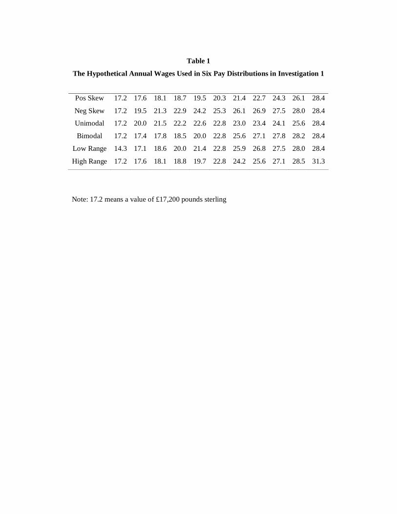
Table 1

The Hypothetical Annual Wages Used in Six Pay Distributions in Investigation 1

Note: 17.2 means a value of £17,200 pounds sterling

Pos Skew 17.2 17.6 18.1 18.7 19.5 20.3 21.4 22.7 24.3 26.1 28.4

Neg Skew 17.2 19.5 21.3 22.9 24.2 25.3 26.1 26.9 27.5 28.0 28.4

Unimodal 17.2 20.0 21.5 22.2 22.6 22.8 23.0 23.4 24.1 25.6 28.4

Bimodal 17.2 17.4 17.8 18.5 20.0 22.8 25.6 27.1 27.8 28.2 28.4

Low Range 14.3 17.1 18.6 20.0 21.4 22.8 25.9 26.8 27.5 28.0 28.4

High Range 17.2 17.6 18.1 18.8 19.7 22.8 24.2 25.6 27.1 28.5 31.3

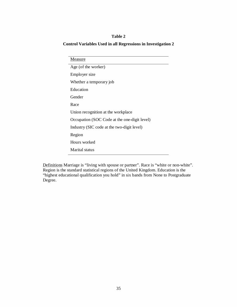
35

Table 2

Control Variables Used in all Regressions in Investigation 2

Measure

Age (of the worker)

Employer size

Whether a temporary job

Education

Gender

Race

Union recognition at the workplace

Occupation (SOC Code at the one-digit level)

Industry (SIC code at the two-digit level)

Region

Hours worked

Marital status

Definitions Marriage is “living with spouse or partner”. Race is “white or non-white”. Region is the standard statistical regions of the United Kingdom. Education is the “highest educational qualification you hold” in six bands from None to Postgraduate Degree.

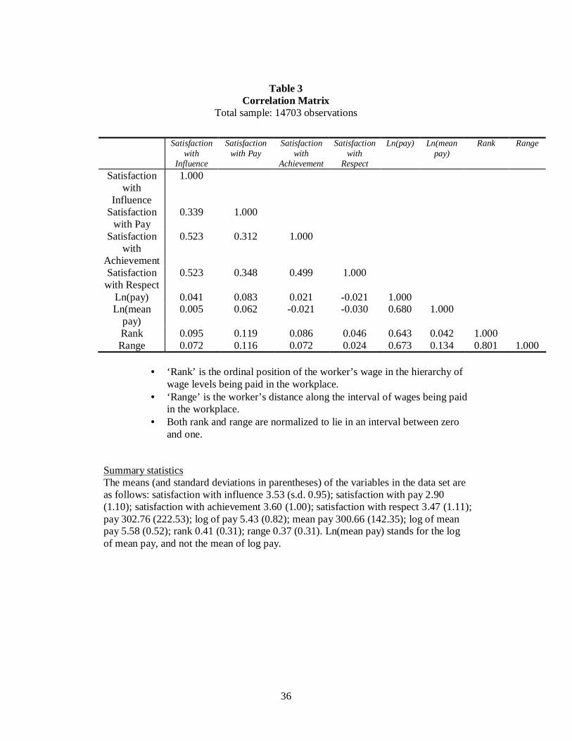
36

Table 3 Correlation Matrix

Total sample: 14703 observations

Satisfaction with

Influence

Satisfaction with Pay

Satisfaction with

Achievement

Satisfaction with

Respect

Ln(pay) Ln(mean pay)

Rank Range

Satisfaction with

Influence

1.000

Satisfaction with Pay

0.339 1.000

Satisfaction with

Achievement

0.523 0.312 1.000

Satisfaction with Respect

0.523 0.348 0.499 1.000

Ln(pay) 0.041 0.083 0.021 -0.021 1.000 Ln(mean

pay) 0.005 0.062 -0.021 -0.030 0.680 1.000

Rank 0.095 0.119 0.086 0.046 0.643 0.042 1.000 Range 0.072 0.116 0.072 0.024 0.673 0.134 0.801 1.000

• ‘Rank’ is the ordinal position of the worker’s wage in the hierarchy of

wage levels being paid in the workplace. • ‘Range’ is the worker’s distance along the interval of wages being paid

in the workplace. • Both rank and range are normalized to lie in an interval between zero

and one. Summary statistics The means (and standard deviations in parentheses) of the variables in the data set are as follows: satisfaction with influence 3.53 (s.d. 0.95); satisfaction with pay 2.90 (1.10); satisfaction with achievement 3.60 (1.00); satisfaction with respect 3.47 (1.11); pay 302.76 (222.53); log of pay 5.43 (0.82); mean pay 300.66 (142.35); log of mean pay 5.58 (0.52); rank 0.41 (0.31); range 0.37 (0.31). Ln(mean pay) stands for the log of mean pay, and not the mean of log pay.

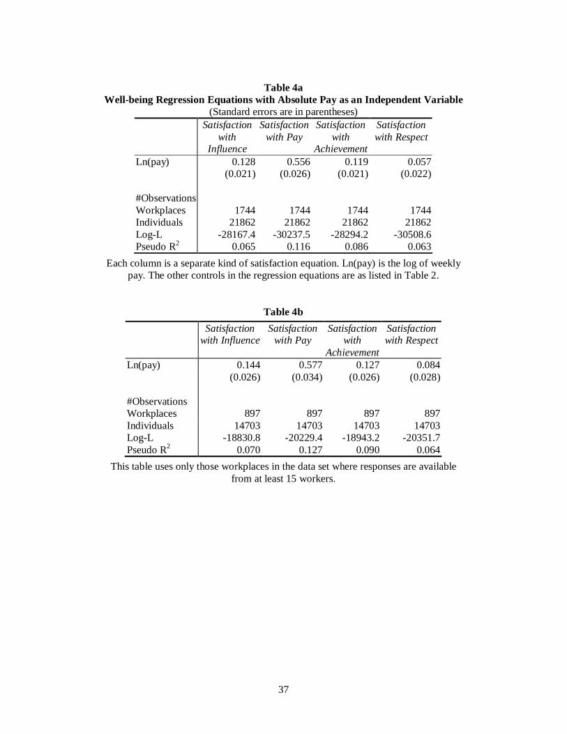
37

Table 4a Well-being Regression Equations with Absolute Pay as an Independent Variable

(Standard errors are in parentheses) Satisfaction

with Influence

Satisfaction with Pay

Satisfaction with

Achievement

Satisfaction with Respect

Ln(pay) 0.128 0.556 0.119 0.057 (0.021) (0.026) (0.021) (0.022) #Observations Workplaces 1744 1744 1744 1744 Individuals 21862 21862 21862 21862 Log-L -28167.4 -30237.5 -28294.2 -30508.6 Pseudo R2 0.065 0.116 0.086 0.063

Each column is a separate kind of satisfaction equation. Ln(pay) is the log of weekly pay. The other controls in the regression equations are as listed in Table 2.

Table 4b

Satisfaction with Influence

Satisfaction with Pay

Satisfaction with

Achievement

Satisfaction with Respect

Ln(pay) 0.144 0.577 0.127 0.084 (0.026) (0.034) (0.026) (0.028) #Observations Workplaces 897 897 897 897 Individuals 14703 14703 14703 14703 Log-L -18830.8 -20229.4 -18943.2 -20351.7 Pseudo R2 0.070 0.127 0.090 0.064

This table uses only those workplaces in the data set where responses are available from at least 15 workers.

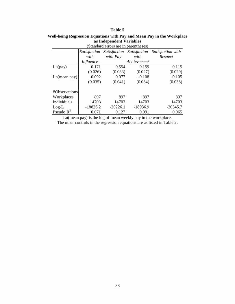
38

Table 5

Well-being Regression Equations with Pay and Mean Pay in the Workplace as Independent Variables

(Standard errors are in parentheses) Satisfaction

with Influence

Satisfaction with Pay

Satisfaction with

Achievement

Satisfaction with Respect

Ln(pay) 0.171 0.554 0.159 0.115 (0.026) (0.033) (0.027) (0.029) Ln(mean pay) -0.092 0.077 -0.108 -0.105 (0.035) (0.041) (0.034) (0.038) #Observations Workplaces 897 897 897 897 Individuals 14703 14703 14703 14703 Log-L -18826.2 -20226.1 -18936.9 -20345.7 Pseudo R2 0.071 0.127 0.091 0.065

Ln(mean pay) is the log of mean weekly pay in the workplace. The other controls in the regression equations are as listed in Table 2.

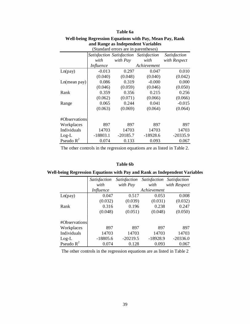
39

Table 6a

Well-being Regression Equations with Pay, Mean Pay, Rank and Range as Independent Variables

(Standard errors are in parentheses) Satisfaction

with Influence

Satisfaction with Pay

Satisfaction with

Achievement

Satisfaction with Respect

Ln(pay) -0.013 0.297 0.047 0.010 (0.040) (0.048) (0.040) (0.042) Ln(mean pay) 0.086 0.319 -0.000 0.000 (0.046) (0.059) (0.046) (0.050) Rank 0.359 0.356 0.215 0.256 (0.062) (0.071) (0.066) (0.066) Range 0.065 0.244 0.041 -0.015 (0.063) (0.069) (0.064) (0.064) #Observations Workplaces 897 897 897 897 Individuals 14703 14703 14703 14703 Log-L -18803.1 -20185.7 -18928.6 -20335.9 Pseudo R2 0.074 0.133 0.093 0.067

The other controls in the regression equations are as listed in Table 2.

Table 6b

Well-being Regression Equations with Pay and Rank as Independent Variables

Satisfaction with

Influence

Satisfaction with Pay

Satisfaction with

Achievement

Satisfaction with Respect

Ln(pay) 0.047 0.517 0.053 0.008 (0.032) (0.039) (0.031) (0.032) Rank 0.316 0.196 0.238 0.247 (0.048) (0.051) (0.048) (0.050) #Observations Workplaces 897 897 897 897 Individuals 14703 14703 14703 14703 Log-L -18805.6 -20219.5 -18928.9 -20336.0 Pseudo R2 0.074 0.128 0.093 0.067

The other controls in the regression equations are as listed in Table 2

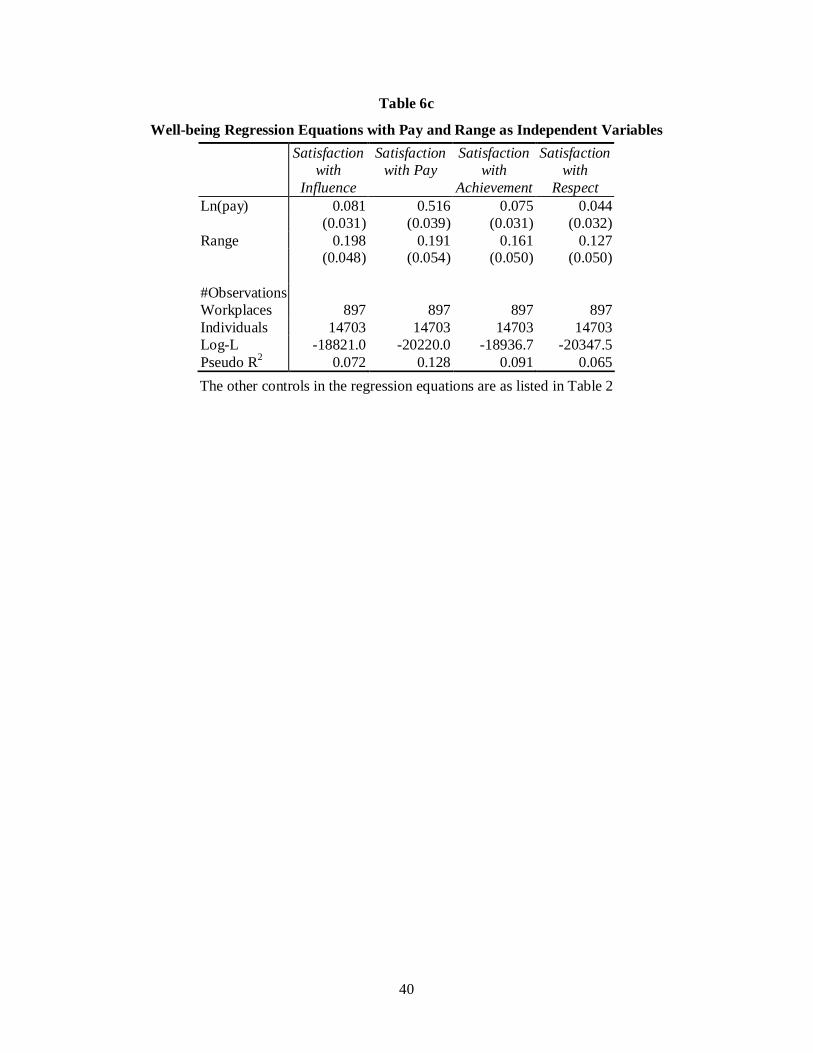
40

Table 6c

Well-being Regression Equations with Pay and Range as Independent Variables

Satisfaction with

Influence

Satisfaction with Pay

Satisfaction with

Achievement

Satisfaction with

Respect Ln(pay) 0.081 0.516 0.075 0.044 (0.031) (0.039) (0.031) (0.032) Range 0.198 0.191 0.161 0.127 (0.048) (0.054) (0.050) (0.050) #Observations Workplaces 897 897 897 897 Individuals 14703 14703 14703 14703 Log-L -18821.0 -20220.0 -18936.7 -20347.5 Pseudo R2 0.072 0.128 0.091 0.065

The other controls in the regression equations are as listed in Table 2

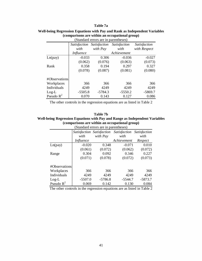
41

Table 7a

Well-being Regression Equations with Pay and Rank as Independent Variables (comparisons are within an occupational group)

(Standard errors are in parentheses) Satisfaction

with Influence

Satisfaction with Pay

Satisfaction with

Achievement

Satisfaction with Respect

Ln(pay) -0.033 0.306 -0.036 -0.027 (0.062) (0.076) (0.063) (0.073) Rank 0.358 0.194 0.297 0.327 (0.078) (0.087) (0.081) (0.080) #Observations Workplaces 366 366 366 366 Individuals 4249 4249 4249 4249 Log-L -5505.8 -5784.3 -5550.2 -5869.7 Pseudo R2 0.070 0.143 0.127 0.086

The other controls in the regression equations are as listed in Table 2

Table 7b Well-being Regression Equations with Pay and Range as Independent Variables

(comparisons are within an occupational group) (Standard errors are in parentheses)

Satisfaction with

Influence

Satisfaction with Pay

Satisfaction with

Achievement

Satisfaction with

Respect Ln(pay) -0.020 0.348 -0.071 0.010 (0.061) (0.072) (0.062) (0.072) Range 0.304 0.092 0.346 0.227 (0.071) (0.078) (0.072) (0.073) #Observations Workplaces 366 366 366 366 Individuals 4249 4249 4249 4249 Log-L -5507.0 -5786.8 -5544.7 -5873.7 Pseudo R2 0.069 0.142 0.130 0.084 The other controls in the regression equations are as listed in Table 2

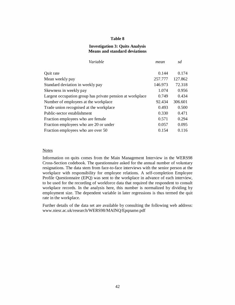
42

Table 8

Investigation 3: Quits Analysis Means and standard deviations

Variable mean sd

Quit rate 0.144 0.174 Mean weekly pay 257.777 127.862 Standard deviation in weekly pay 146.973 72.318 Skewness in weekly pay 1.074 0.956 Largest occupation group has private pension at workplace 0.749 0.434 Number of employees at the workplace 92.434 306.601 Trade union recognised at the workplace 0.493 0.500 Public-sector establishment 0.330 0.471 Fraction employees who are female 0.571 0.294 Fraction employees who are 20 or under 0.057 0.095 Fraction employees who are over 50 0.154 0.116

Notes

Information on quits comes from the Main Management Interview in the WERS98 Cross-Section codebook. The questionnaire asked for the annual number of voluntary resignations. The data stem from face-to-face interviews with the senior person at the workplace with responsibility for employee relations. A self-completion Employee Profile Questionnaire (EPQ) was sent to the workplace in advance of each interview, to be used for the recording of workforce data that required the respondent to consult workplace records. In the analysis here, this number is normalized by dividing by employment size. The dependent variable in later regressions is thus termed the quit rate in the workplace.

Further details of the data set are available by consulting the following web address: www.niesr.ac.uk/research/WERS98/MAINQ/Epqname.pdf

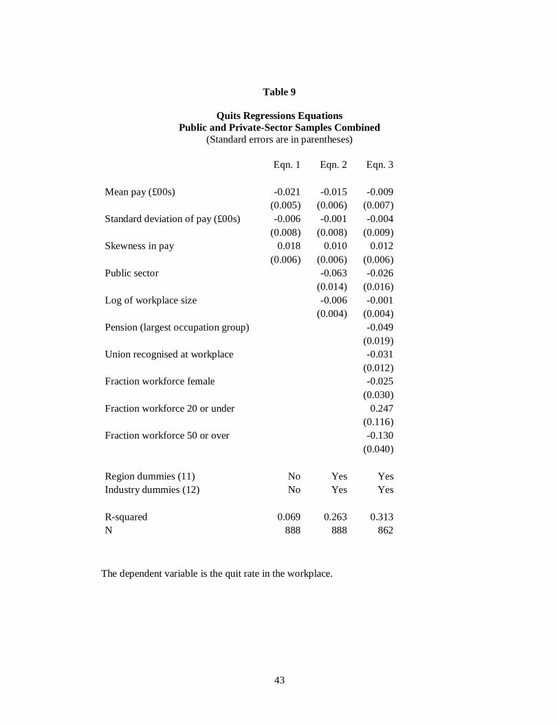
43

Table 9

Quits Regressions Equations Public and Private-Sector Samples Combined

(Standard errors are in parentheses)

Eqn. 1 Eqn. 2 Eqn. 3 Mean pay (£00s) -0.021 -0.015 -0.009 (0.005) (0.006) (0.007) Standard deviation of pay (£00s) -0.006 -0.001 -0.004 (0.008) (0.008) (0.009) Skewness in pay 0.018 0.010 0.012 (0.006) (0.006) (0.006) Public sector -0.063 -0.026 (0.014) (0.016) Log of workplace size -0.006 -0.001 (0.004) (0.004) Pension (largest occupation group) -0.049 (0.019) Union recognised at workplace -0.031 (0.012) Fraction workforce female -0.025 (0.030) Fraction workforce 20 or under 0.247 (0.116) Fraction workforce 50 or over -0.130 (0.040) Region dummies (11) No Yes Yes Industry dummies (12) No Yes Yes R-squared 0.069 0.263 0.313 N 888 888 862

The dependent variable is the quit rate in the workplace.

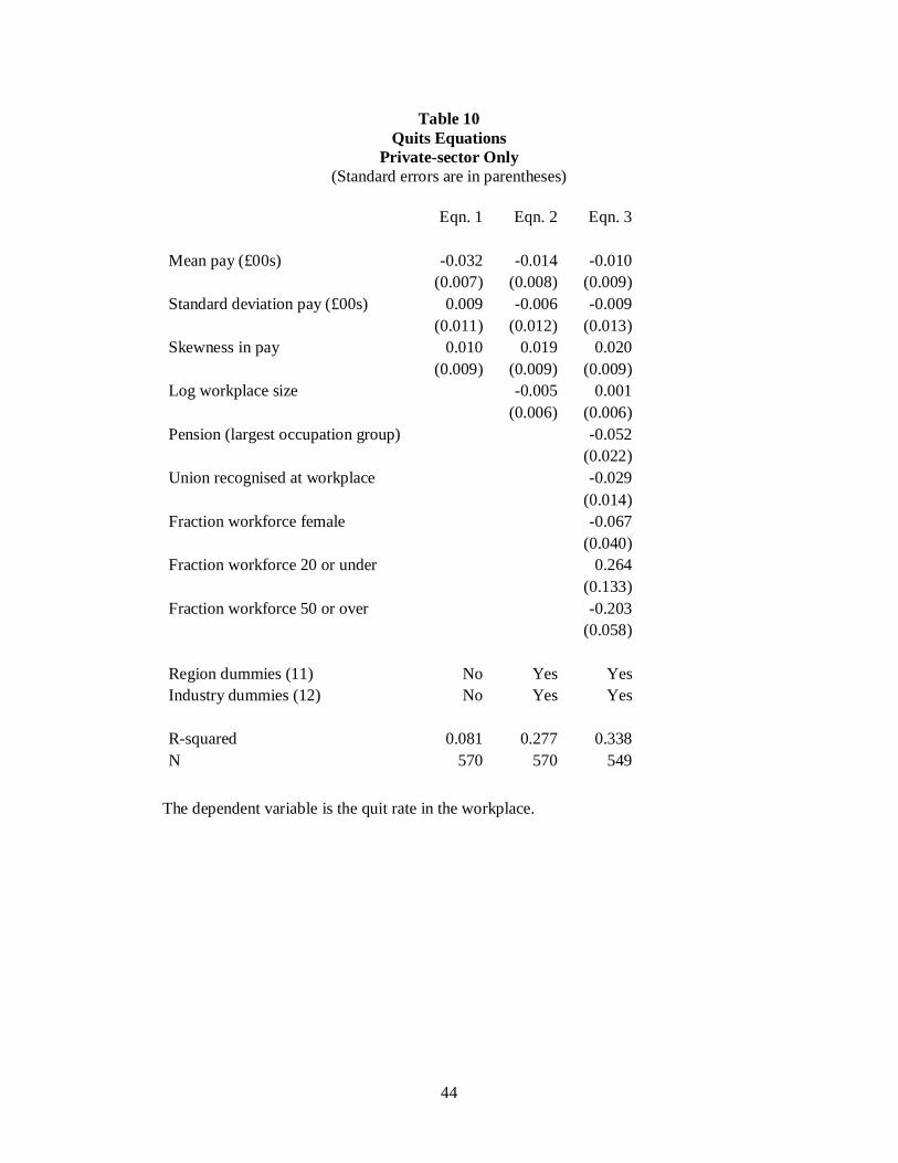
44

Table 10 Quits Equations

Private-sector Only (Standard errors are in parentheses)

Eqn. 1 Eqn. 2 Eqn. 3 Mean pay (£00s) -0.032 -0.014 -0.010 (0.007) (0.008) (0.009) Standard deviation pay (£00s) 0.009 -0.006 -0.009 (0.011) (0.012) (0.013) Skewness in pay 0.010 0.019 0.020 (0.009) (0.009) (0.009) Log workplace size -0.005 0.001 (0.006) (0.006) Pension (largest occupation group) -0.052 (0.022) Union recognised at workplace -0.029 (0.014) Fraction workforce female -0.067 (0.040) Fraction workforce 20 or under 0.264 (0.133) Fraction workforce 50 or over -0.203 (0.058) Region dummies (11) No Yes Yes Industry dummies (12) No Yes Yes R-squared 0.081 0.277 0.338 N 570 570 549

The dependent variable is the quit rate in the workplace.

45

Figure Captions

Figure 1. Two hypothetical distributions to illustrate the predictions of rank-

dependence.

Figure 2. The six stimulus distributions used in Experiment 1.

Figure 3. Data (symbols) and fit of the range-frequency model (solid lines) for the six

different distributions used in Experiment 1. Each data point represents the mean of

24 observations.

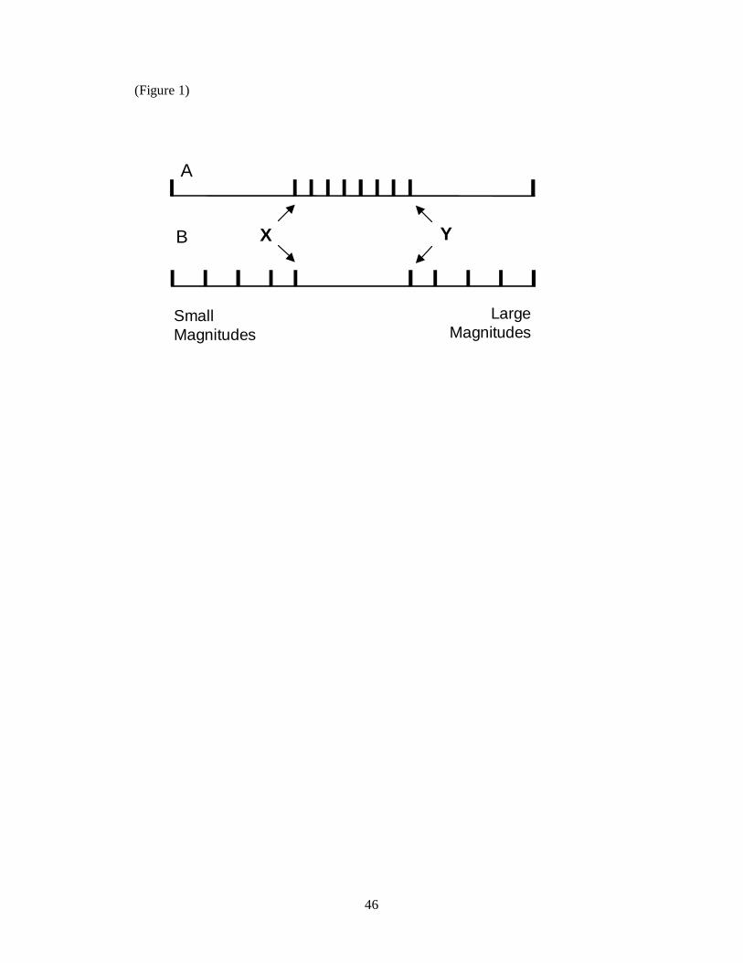
46

(Figure 1)

A

B X Y

SmallMagnitudes

LargeMagnitudes

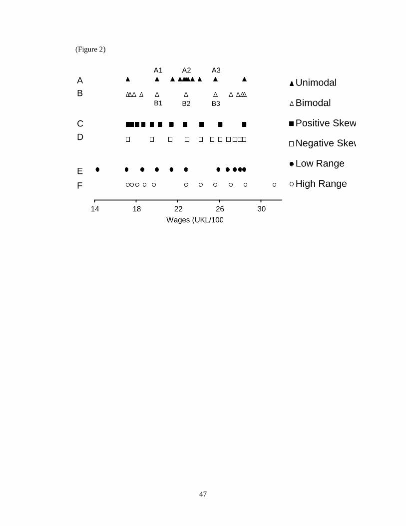
47

(Figure 2)

14 18 22 26 30

Wages (UKL/1000)

Unimodal

Bimodal

Positive Skew

Negative Skew

Low Range

High Range

AB

C

D

E

F

B1 B2 B3

A1 A2 A3

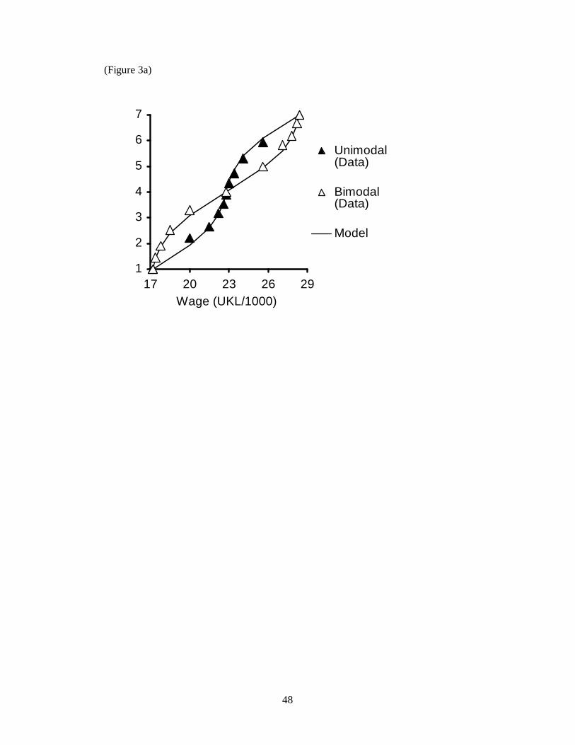
48

(Figure 3a)

1

2

3

4

5

6

7

17 20 23 26 29Wage (UKL/1000)

Unimodal(Data)

Bimodal(Data)

Model

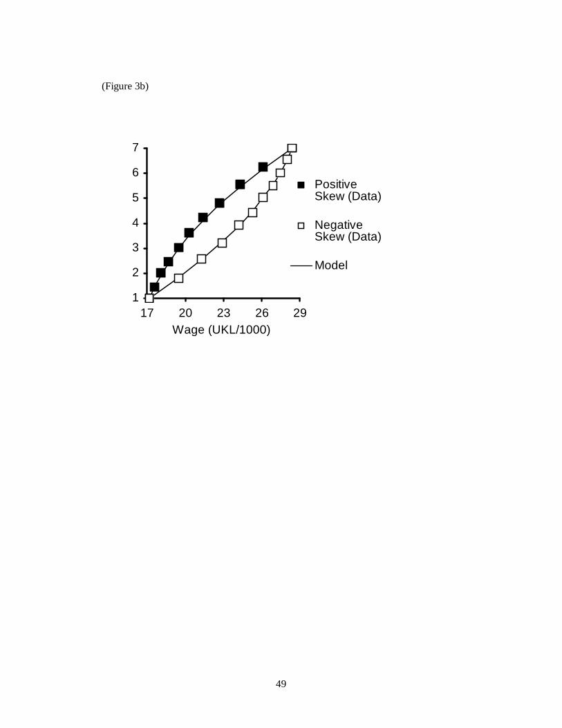
49

(Figure 3b)

1

2

3

4

5

6

7

17 20 23 26 29Wage (UKL/1000)

PositiveSkew (Data)

NegativeSkew (Data)

Model

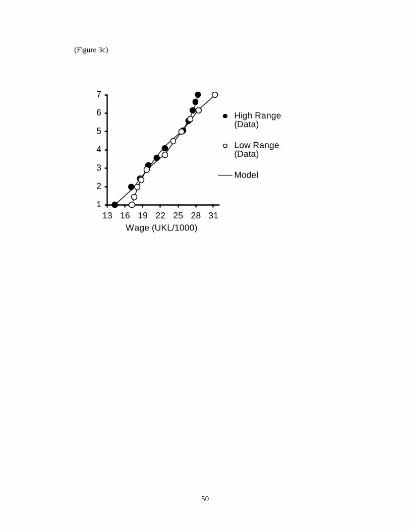
50

(Figure 3c)

1

2

3

4

5

6

7

13 16 19 22 25 28 31Wage (UKL/1000)

High Range(Data)

Low Range(Data)

Model