c

UNIVERSITÉ de BRETAGNE OCCIDENT ALE

U. E. R. DES SCIENCES DE LA MATIÈRE ET DE LA MER

THE SE

PRÉSENTÉE POUR OBTENIR LE TITRE DE

Doèteur de 3e Cycle

Spécialité OCEANOGRAPHIE PHYSIQUE

PAR

A.S. UNNIKRISHNAN

NUMERICAL MODELING TECHNIQUES FOR THE STUDY OF

HORIZONTAL CIRCULATION IN ESTUARIES

APPLICATION TO THE GIRONDE

Soutenue Je 4 Février 1985 devant la commission d'examen

Monsieur J.C. SALOMON Professeur, Université de Bretagne Occidentale

Messieurs G. PASCAL· - Professeur, Université de Bretagne Occidentale

P. CASTAING Assistant, Université de Bordeaux 1

R. MAZE Maître Assistant, Université de Bretagne Occidentale

J.L. MAUVAIS Chef du Département ELGMM, IFREMER, Brest

IFREMER Bibliotheque de BREST

11111111111111111111111111111111111111111111111111 OEL07919

} Président

Examinateurs

UNIVERSITÉ de BRETAGNE OCCIDENT ALE

U. E. R. DES SCIENCES DE LA MATIÈRE ET DE LA MER

Tuc ce 1 IL .. '-1

PRÉSENTÉE POUR OBTENIR LE TITRE DE

Docteur de 3e Cycle

Spécialité : OCEANOGRAPHIE PHYSIQUE

PAR

A.S. UNNIKRISHNAN

NUMERICAL MODELING TECHNIQUES FOR THE STUDY OF

HORIZONTAL CIRCULATION IN ESTUARIES

APPLICATION TO THE GIRONDE

Soutenue le 4 Février 1985 devant la commission d'examen

Monsieur J.C. SALOMON Professeur, Université de Bretagne Occidentale } Président

Messieurs G. PASCAL Professeur, Université de Bretagne Occidentale

P. CASTAING Assistant, Université de Bordeaux 1 Examinateurs

R. MAZE Maître Assistant, Université de Bretagne Occidentale

J.L. MAUVAIS Chef du Département ELGMM, IFREMER, Brest

).

ACKNCWLEDGEMENTS

I express my thanks to Prof. LE FLOCH who welcomed me to this·

laboratory and provided ~~e necessary facilities.

I wish to express my deep sense of gratitude to Prof. J.·c.

SALOMON, who has be en guiding me throughou.t the duration of three years of

work.

I would like to thank Prof. G. PASCAL, Professer, Université de

Bretagne Occidentale, Dr. J.L. ~AUVAIS, Head of the department of ELGMM,

IFREMER, Brest, Or. Ré ~AZE, Maitre Assistant, Université de Bretagne Occiden­

tale and or. P. CASTAING,Assistant, Université de Bordeaux I who have given

me the honour of participating in the committee of examiners.of the thesis.

I express my thanks to the Port Autonome de Bordeaux for giving

me an authorisation to consult the documents of the Laboratoire National

·d'Hydraulique about the Gironde estuary.

My sincere.thanks are to all the collegues of the laboratory who

have always encouraged me. In particular, I thank Dr. G. ROUGIER, Dr. v. MARIETTE, Dr. G. LANGLOIS and Mr. s. GHIRON, with whom I had useful discussions

often.

The services made by Mr. P. OO.P.RE and Mr. R. MARCHERON, IFREMER

in preparing the diagrams are acknowledged.

Finally, I thank Miss Pascale MAZO, Who patiently typed the ma-

nus cri pt.

The financial assistance in the form of a fellowship awarded by

the Ministry of External Affaires, Gov. of France under the Indo French cul­

tural ex change programme is duly acknowledged •.

CONTENTS

INTRODUCTION

CHAPTER I DESCRIPTION OF THE GIRONDE ESTUARY

I. Introduction

II. Geomorphology

III. River discharges

IV. Tides and tidal currents

CHAPTER II DESCRIPTION OF THE NUMERICAL METHODS USED

CHAPTER III

I. Review of literature

II. Application of a two dimensional madel

in the horizontal plane

III. Link node madel

IV. Irregular grid finite difference madel for

estuarine applications

CIRCULATION IN THE GIRONDE

Introduction

PART I - WATER SURFACE ELEVATION

I. Introduction

4

4

6

7

8

9

14

20

27

28

)

1

II. Calibration 28

III. Longitudinal variations 28

IV. Lateral variations 35

PART II - CIRCULATION

I. Introduction 43

II. Brief review of circulation studies in the

Gironde 43

III. Discussion of simulation results 47

IV. Comparison between observed and computed currents 54

V. Conclusion 59

Appendix I

Appendix II

Appendix III

CHAPTER IV RESIDUAL CIRCULATION IN THE GIRONDE

I. Introduction

II. Residual circulation studies in the Gironde

III. Depth averaged residual parameters

IV. Conclusion

CONCLUSION

APPENDIX IV. PERFORMANCE OF DIFFERENT MODELS IN TERMS OF COMPUTATIONAL

ASPECTS

BIBLIOGRAPHY

1 16

1 16

1 19

131

132

134

135

INTRODUC'PION

- 1 -

Recent advances in fast computers have helped in developing

numerical models for the study of estuarine and coastal dynamics. Sc far, 1

different workers have·made definitions of an estuary mainly based on

salinity considerations. For example, following PRITCHARD (1965), an

estuary may be defined as "a semi enclosed body of water having a free

connection with the open sea within which sea water is mesurably diluted with

fresh water derived from land drainage". In the case of european estuaries,

which are caracterised by high tidal ranges, the tidal action extends well

beyond the penetration of salinity. SALOMON (personal communications),

gives a more appropriate definition for the limits of an estuary as follows

at the mouth, where a cross sectional line shows the influence of river

by a slight decrease of salinity and at the head, where the periodic

oscillations of water surface elevation disappear.

The necessity of learning estuarine dynamics is becoming increa­

singly important because of navigational purposes 1 sedimentological appli­

cations, pollution resulting from industrial discharges, thermal pollution

due tc the discharge of heat from nuclear power plants etc. The estuarine

water: are highly nutrient rich and they are the spawning grounds for many

fishes and the nursing grounds for many ethers. Bence any damage tc the

environment will cause subsequent effects on fish production.

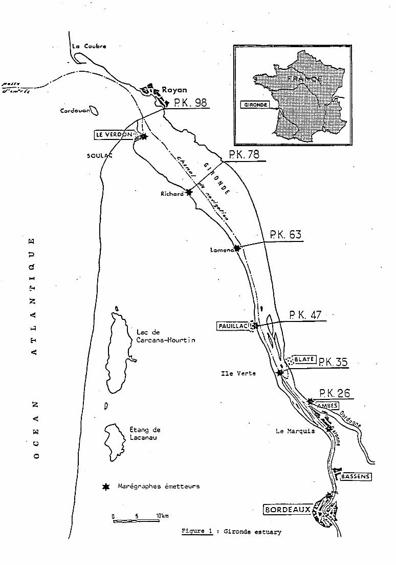
The Gironde estuary(fig 1), situated at the southwestern part of France,

near Bordeaux, has been an abject of study since a number of years. This estu-

ary is.caracterised by a number of channels, longitudinal bars and islands.

Historically, along the Gironde, there had been deposition of sediments in 1

seme regions and erosion in seme ether parts, where as certain regions-have

·suffered alternate erosion and deposition. In arder tc learn the sedimen­

tation problems, various workers have studied the circulation patterns based

on the numerous observations available about the hydrology and currents.

These measurements were carriedoutmainly by the Port Autonome de Bordeaux

(P. A. B.), Institut Géologique du Bassin d'Aquitaine and the Electricité de

France, besides the systematic data obtained from different tide gauges

installed by P. A. B.

Recently, the E. o. F. has decided tc choose the median channel

at PK 52 of the e~tu~nr f~r. thermal discharcres from the nuclear power. nlant

of Braud-et-Saint-Louis. This also has arisen a lot of interest among different

-~

z <

z < ~

0

0

ta Coubre

Cordouan\J

D

Lac de Carcans-Hourtin

)\Etang de v lacanau

~ Marégraphes émetteurs

0 5 10km ~~i:=;;;;:;;;;;;;o

P. K. 47

Ile Verte

!BORDEAUX

Figure 1 Gironde estuary

•

- 3 -

workers in studying this estuary.

In this study, we ~ttempt to develop numerical models to study

the horizontal circulation in the Gironde. This involves the computation of

depth averaged tidal currents and water surface elevations and to study the

lateral variations of these physical parameters during a tidal period. The

models used are two dimensional in the horizontal plane (x-y directions) •.

In order to take into account of the geomorphological peculiarities of the

estuary, such as the pr~sence of channels and islands, we.have used different

numerical methods in modelling. The second objective of this work is to

compare the relative advantages and disadvantages of the different techniques

used •

CHAPTER I

DESCRIPTION OF THE GIRONDE ESTUARY

- 4 -

I. INTRODUCTION

The Gironde estuary is formed by the junction of two·rivers,

Dordogne and the Garonne. It is the largest of the French estuaries in

area (450 km2

during high tide). The rivers Dordogne and the Garonne

drain from the Pyrènées and the Massif Central respectively. The total

drainage basin (74000 km2) is the fourth largest in France, after the Loire,

the Rhône, and the Seine.

II. GEOMORPHOLOGY .

The Gironde is caracterised by a regular geometry with its breadth,

mean depth and surface area decreasing exponentially tow~a:rds the head.

The distances are marked in kilometers as •rpoi~t kilométrique" (P.K-.)

from the pointe de Grave towards the head. A detailled examination of the - -

bathymetrie chart of-the Gironde reveals the following features.

1) Lower estuary

The lower estuary is caracterised by a typical two channel

system with the navigation channel at the southern side and the Saintonge

channel at the northern side .(figure 2). The two channels are separated by

regions of sand bars. The depth in the southern channel varies between 6 to

8 m. At PK 81, there is a break in its slope and downstream further, the

depth increases. The Saintonge channel is wider and its depth is of-the order

of 3 to 5 m. From PK 80 onwards, its depth increases. Towards the mouth,

the navigation channel marges with the northern channel where the depths

attain upto 30 metres.

Between PK 91 and PK 78, there are a series of longitudinal bars

situated in between the two principal channels. They are called "banc de

Marguerites", "banc de Talais", "banc de Mets" and "banc de Goulée" in the or­

der from PK 91 onwards towards the head. Besides, near PK 70 there is a

submerged dike called" digue de Valeyrac':

d~s

Bo.ne det Talais

Banc de Mets

nanc de

/ '<-} P1(70

St. Christoly

Figure 2

- 5 -

E~n~ èe St-Est~pho

Pl(. 60 -

I.lœ Tro~:~poloup

Pk. so

Pouillac

rain

1 N

.J.

d'Ambès

0 ~--;.,._ __ _ D ·Zonas ,

int·ertidües

1>'="''::·,1· o 5mtod . '1

0 5 -10 m..., ~ 0 . = Q.

mill] 10 -20 m ~ '1 1:11 f;,iiJ > 20 m

Bathymetrie charts of the estuary a lower estuary b upper estuary (in, TESSON GILET, 1981)

• 1

'

- 6 -

2) Upper estuary

The.upper estuary is the region between Bec d'Ambes and St

Christoly approximately. The geomorphological peculiarity of this region

is the presence of numerous islands and longitudinal sand banks. Between

Bec d'Ambes and Ile Verte, the principal channel is situated along and

right side of a series of islands such as Ile cazeau, Ile du Nord and

Ile Verte. Downstream, up to St Christoly, tne navigational channel con­

tinues along the southern side. Its depth is in between 7 to 10 m and

breadth 400-800 m. The Blaye channel starting from PK 35 onwards towards

the mouth is less wide and the depths are of the order of 5 m, with a

maximum of 10 m at Blaye. Still further towards the mouth of the estua­

ry, the northern channel is situated between the "banc de St Louis" and

the north bank. Between Blaye and PK 50, there a series of islands name­

ly, "Ile Sans Pain", "Ile Bouchaud", "Ile Patiras" and "Ile St Louis",

situated in between the two principal channels. Downstream of PK 50,

there are two main longitudinal sand banks, "banc de St Louis", be.tween

PK 50 and PK 55 approximately and "banc St Estephe" near PK 60, the former

situated near the northern channel and the latter near the southern

channel.

III. RIVER DISCHARGES

ALLEN (1972) gives the following figures for the river discharge

rates of the Garonne and the Dordogne. These figures are calculated between

1961 and 1970.

3 The mean discharge rate of the Garonne is 444 m /s, with a maxi-

mum of 854 m3/s in January and a minimum of 96 m3/s in August. In the case

of Dordogne, the mean value·is 322 m3/s with a maximum of 598m3/sin

January and a minimum of 139 m3/s in August.

Recent studies made by the P .A.B. (FERAL. et al., 1982) show

that the discharge rates are higher than those mentioned above.

It is estimated that the ratio of the tidal prism to the volume

of water introduced by the rivers is more than 500 when the total discharge

- 7 -

rates are less than 500 m3/s, where as in the case of exceptionally high

river flow rates (7500 m3/s), this ratio is of the order of 10 (CASTAING,

1981).

IV. TIDES AND TIDAL CURRENTS

Tides are sem! diurnal in the Bay of Biscay (period of 12 hours

and 25 minutes). Measurements by CAVANIE and HYACINTHE (1976) at a few stations

near 200 m. isobath show that the tidal range varies between 1.50 to 2 m.

during neap 4ide (coeff. 40 to 50), while during spring tide (coeff. 77

to 86) the range attains 3.50 m. Near the mouth of the Gironde, the tidal

ranges are almost same at Cordouan and Coubre and is about 0.20 m. less than

that of the Pointe de Grave (FICEOT, 1916). There is a tide gauge station

at Cordouan (Fig. 1), through there are no stations near the north bank side.

Eowever, a few surface elevation measurements made by P.A.B. exist at Royan

near the north bank side. A co tidal line passing near Cordouan (Fig. 15)

indicates that the tidal wave comes from western direction before entering

into the estuary.

The variations of surface elevations and currents inside the es­

tuary will be discussed during the course of this dissertation. Eere, it is

only mentioned that the magnitudes of tidal currents at the surface are of

the order of 1-2 m/sec, depending on the coefficient of tide and river flow

rates.

CHAPTER II

DESCRIPTION OF THE NUMERICAL

METHODS USED

- 8 -

This chapter deals with two aspects (Il a brief review of the

different numerical methods existing for the calculation of tidal currents

in the littoral zone and (II) a description of the various numerical tech­

niques used in this work.

I. REVIEW OF LITERATURE

There exists various numerical techniques for computing tidal·

currents in the estuarine and coastal zone. He re, 'Ire discuss mainly

2D models in the horizontal plane. One of the main problems facing a

numerical modeller is in giving a good representation of the coastline.

The classical method consists of ~ rectangular grid with the coastline

approximated by a stair step boundary, and the equations being solved

with a ·finite difference scheme. An example of this method is given by

SALOMON (1976). The method will be discussed in detail later, in this chap­

ter. This technique has the disadvantage of giving a poor representation

of the coastline often resulting in poor values very near the coast.

In order to overcome this difficulty, certain workers have used

the finite element method which uses meshes of variable dimensions usually

triangular. The method described by CONNOR and WANG (1973) may be briefly ...

summarised as follows. It consists·of solution of boundary value problem

with a function of piece wise continuous polynomials. The entair domain

is discretised into a system of finite elements. The elementsatre triangular

in their method and the nodes are the vertices of the triangles. The values

of the variables in the elements are assumed to be a linear function of the

values at the nodes. The whole domain is treated by summation of the contri­

butions of each element. However, finite element methods are found to be

computationally expansive and need a lot of comouter memory space. In the

method of CONNOR and WANG, the authors point out that it needs 4·5 memory

locations to describe eacn nôdal pciint.

PEABSON and WINTER (1977) used a modified scheme in order to mini­

mise the computational expense s of the fini te element technique. l\ brief

account of the method is as follows. The time dependent equations are written

by a set of modal equations obtained by fourier decomposition, except for the

- 9 -

non linear terms which are treated by an iteration technique. The boundary

value problem is then rephrased in terms of variational principles. The va­

riational principle is then used together with a finite element method for

the solution of the variables.

Another approach consists of an application of a hydraulic model,

commonly referred to "link-node IJPdel". The method was utilised by KENNETH D.

FEIGNER et.al (1970) for the San Fransisco delta systems. In this method, the

grid network consists of polygons of variable dimensions whose centres of gra­

vi ty are call ed j unctions. Any two j unctions are connected by a "channel

element". The method consists of calculating velocities for the channel

elements using the equation of momentum in the one dimensional form and the

water surface elevations are computed at the junctions based on the flux

of water entering and leaving a polygon. The method uses an explicit finite

difference scheme. In 1978, LANGLEY R. MUIR used a similar principle with

an implicit scheme for estuarine applications.

THACKER (1979), used a scheme called "Irregular grid finite

difference scheme" for the forecast of storm surfaces. This method is simi­

lar to the finite element technique, as far as the grid net work is concerned,

but the equations written in finite difference form. This scheme will be

discussed in detail later, in this chapter.

II. APPLICATION OF A TWO DIMENSIONAL IV!ODEL TN TEE HO?..IZONTAL PLANE

Here, we apply a two dimensional model in the horizontal plane

using a rectangular grid and the coastline represented cy a stair step

boundary. Hereafter, this model is referred to "stair step boundary model" •

. for the sake of notation. The model was developed for the French estuaries by

SALOMON ( 1976) •

The model consists of e{uations of momentum and continuity inte­

grated in the vertical plane, ~fter being integrated over a very small inter­

val of time, initially, in order to eliminate aleatory movements.

~+ at 0au + rx

vau _ ô y fV + 3~+

9àX

~+ ôt . U~+ a x v:av +

a y fU + 3 z; 9!y

3 z; - + at

3 (HU) + 3 (HV) = O ôx ôy

where

U and V

h

H= h + z;

g

f

c

AU, AV

gU

+ gV

- 10 -

(U2 + c2 H

(U2

c2

1 V2)2 't'

sx e:t..U • 0 ( 1-) + -+ pS

1

+ V2) Ï + 't' sy + e:t..V - 0 (2} pH

H

(3)

the vertically integrated values of

velocity components in the x and.y

directions, the integration being carried

out between - h to z;

depth of hottom

water surface elevation

total depth of water

acceleration due to gravity

coriolis parameter

coefficient of Chezy

wind stress components in the x and y

directions

coefficient of pseudo viscosity

Laplacians of velocities U and v.

- 11 -

x and y are the cartesian coordinates in the horizontal plane

and t is the time.

Equations (1) and (2) are the equatior~of momentum in the x and y

directions and (3), the equation of continuity. The terms e: fj, u ande: fj,V are

the terms of pseudo viscosity, introduced in the model by SALOMON, in arder

to dissipate small wave length energy.

The bottom friction is parameterised in terms of the coefficient of

Chezy, by the following relation based on the hypothesis of PRANDTL. The coeffi­

cient of Chezy is a function of the total height of water column.

C • 7.83 Log (0.37 H/ ) Zo {4)

where Zo is the thickness of rugosity.

The wind stress components in the x and y directions are given as

follows.

T

T

where

pa CD (u - U) = sx x

sy pa CD (u - V) y

density of air

drag coefficient'

~eux.- 2 U) + (u

y V)2

~(ux .. - U) 2 + (u V)2 y

wind velocities in the x and y directions.

1) Numerical Resolution

(5)

(6)

The madel uses an implicit in alternate direction scheme. This nume­

rical scheme was introduced by PEACEr~N and RACHFORD in meteorology. The prin­

ciple of the method is as follows.

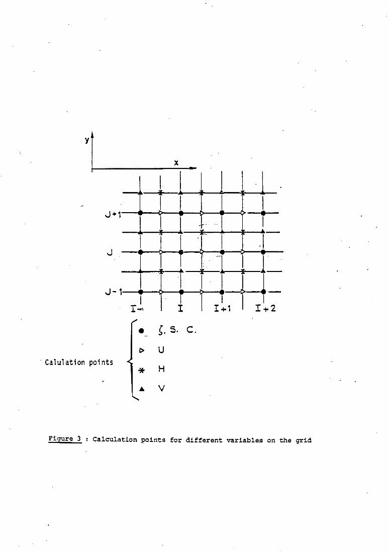
In the computational grid, u, V and ~ are calculated at different

points as shawn in figure 3.

Y~+------x --

J

J-1

I

· Calulation points

1

T1 1

1 _,

•

i T ~ .:...

T I

~. s. c .

u

H

v

1 1

1 1

- ... 1 ~ ---

1 .1 : ~ ...

-1 -

1 Io~-1 I+2

Figure 3 Calculation points for different variables on the grid

- 13 -

The computation procedure may be described briefly as follows.

For the first half time interval, the equation of momenturr in the x direction

and the equation nf continuity are solved for each row of the matr ix •

The variables situated at the row concerned are treated implicitly, while the

variables situated at the adjacent rows are solved explicitly. For the next half

timé interval, the momentum equation in the y ëir.ection and the equation of

continuity are solved for each column of the matrix in a similar manner. The

equations ( 1) to ( 3) can be written in finite difference form and may be ex­

oressed as tridiaganal matrices. Finally, the solution is made by an inversion

of matrix.

2) Stability

I~ENDERTf:E (1971) showed that the scheme is unconditionally

stable, when the equations are linearised. When non linear terms are in­

cluded, the stability is governed by the following relation.

2 ~t < 2g (~x)

c2 HU (7)

3) Conservation

The system is conservative for a constant topography. In the case of

variations in depths, an oscillation of small wave length was observed in the

case of the Seine (SALOMON, 1980). This is overcome by the introduction of

the pseudo viscosity as discussed earlier.

4). Application

In the present wark, the madel is applied to the Gironde estuary

in the following manner. The entair domain consists of a matrix of 93•20 grid

points. Each of the rivers, namely, Dordogne and the Garonne is represented

by a one dimensional madel and they are connected to the 2D madel. This method

was utilised by SALOMON in the case of the Loire. The lD models fa·r the Dordogne

and the Garonne consist of 94 and 74 grid points respectively. In the 10 models,

tx is the same as in the 2D madel and ~y is varies according to the breadth of

the section concerned.

In the Gironde, the reference point of depths i.e, the lowest law

water mark of ~ivellement General de la France (N. G. F.) varies irre­

gularly from the p,inte de Grave tow~r~s the head of the estuary. The

1owest law water mark at the Pointe de Grave is used as a reference

- 14 -

point and the depths are corrected accordingly so as to bring all the depths

of the domain to a horizontal plane. The grid spacing is 960 metres and the

time step used is 180 seconds. The value of the coefficient of viscosity chosen

is 850 and it is the same troughout the domain.

5) Open boundary conditions

The seaward boundary conditions are given in terms of water surface

elevations. This is done supposing that the tidal wave enters in the form of

an arc of a circle, with the amplitude varying as a sinusoidal function and the

phase determined by the distance from the centre of the arc The amplitudes

are defined based on the tide gauge data at Cordouan. It is true that this

method of defining the open bound~ry conditions needs more precision. Limitations

lie in the fact that the tidal variations near the seaward boundary are known

only at one point, namely Cordouan. At the river sides, the open boundary

conditions are given in terms of the river discharge rates.

I!I. LINK NODE MODEL

The second type of modcl u~ed in the present study is a hydraulic

model, commonly referred to as link node model. This type of model is origi­

nally designed to describe the flow in open channels, where the flow is mainly

one directional. We have chosen the method described by FEIGNER, which is

briefly described in page 9, for the application of the Gironde estuary. The

·model is one dimensional. By laying a grid netw~rk of polygons of variable

sizes, two dimensional aspects of the flow can be represented.

1) Model equations

The model consists of momentum equation in one dimensional form

applied to the channel elements and the equation ~f continuity to the june­

tiens.

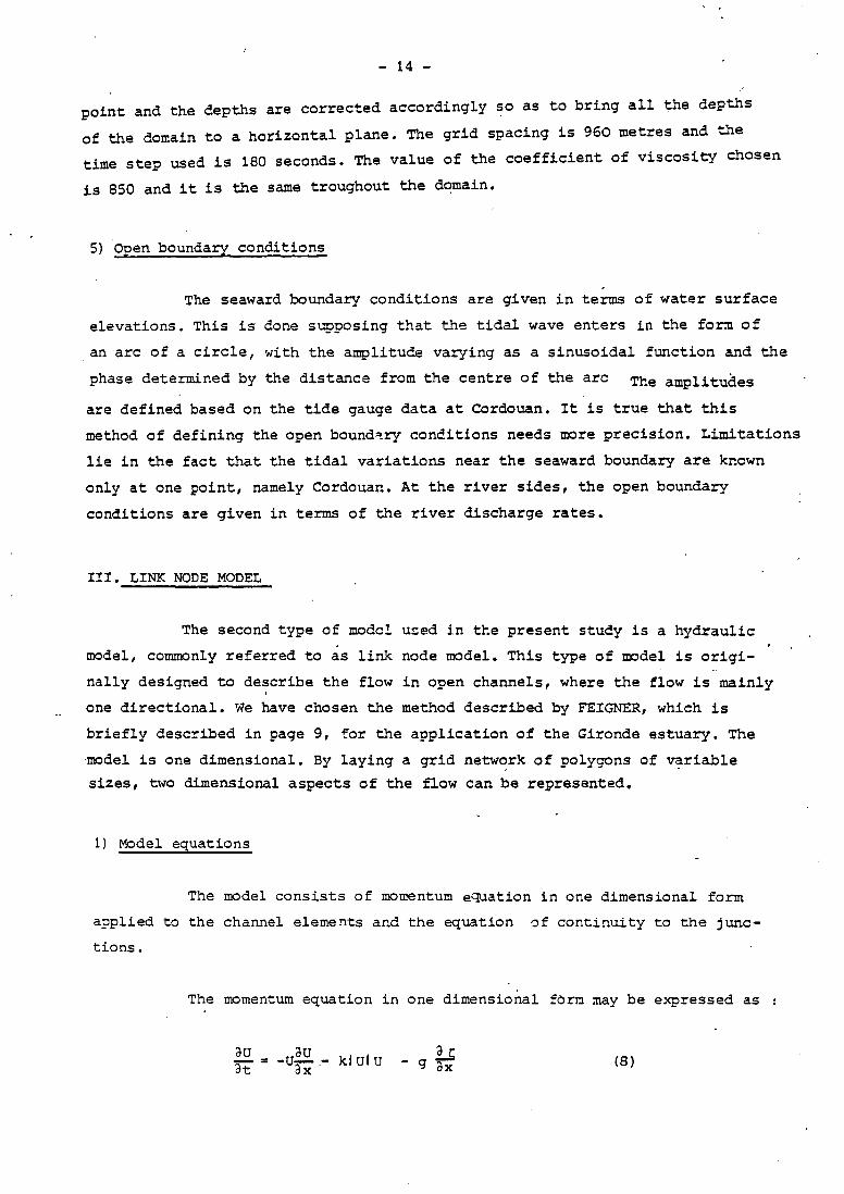
The momentum equation in one dimensional fèrm may be expressed as

au au at= -uax.- klutu ~ - g ax (8)

where

u K

z;

velocity along the channel element

coefficient of friction

water surface elevation

the direction x is taken positive towards the head of the estuary.

The equation of continuity is written as

- 1 ô E"ax

(UA) (9)

It is to be noted that in applying this hydraulic mode! to the

case an estuary, the following assumptïons are madg·.

(i) The wind and Coriolis forces are negligible.

(ii) The parameters like velocity, depth and area of cross section are

constant for a channel element.

(iii)

(iV)

(V)

(Vi)·

A channel element is a straight line.

The cross sectional area is uniform along a channel.

The tidal wave length is at least twice the channel d~pth.

Acceleration normal to the direction of the channel element is

neglected.

Since velocity is constant for à channel element, adve.ction term

cannet be evaluated directly. FEIGNER c9mputed the advection term indirectly

using the continuity equation by a method proposed by LAI (1966).

Expanding (9) and rearranging the terms,

( 10)

where

b m~an channel width

A area of cross section of the channel element.

~ 16 -

2) Method of Resolution

follows

The equations ( 8 ) can be written in finite difference form as

6.Ui 6.Ui fi= -ui x

1

6.z; - ku fu·l -q-i J. x1

(11)

where i indicates the index of the channel element.

The equation of continuity ( 9 ) becomès :

- ( 12) A

n

where n is the index of the junction and 1: -Qn is the algebraic sum of the

flux of water enterinq and leaving a· polyqon and A is the surface area n

of a polygon.

3) Computation procedure

(i)

(ii) ..

(iii)

It involves the following stages

Velocities are calculated for the éhannel elements at time

t+6. t~ using the momentum equation based on the initial conditions

at time t. The initial conditions are the velocities, cross sec­

tional areas and water surface elevations.

Flux of water through each side of a polygon is calculated at

t+6t/z using the velocities obtained above and the cross sectional

areas at t.

The water surface elevations are computed at t~ t/2 based on the con­

tinuity equation using the flux obtained in the second stage.

(iV) The cross sectional areas are calculated at t+6.t/2 using the water

surface· f'Ü~vations comnuted in t:l-to::- t:,i.rd .-;taqe.

(V)

- 17 -

The velocities are computed at t+~t utilising the cross sectional

areas and water surface elevations at t~ t/. . 2

The procedure is continued for the following time step~.

4) Stability

The explicit nature of calculation makes a constraint on the time

step given by the following relation.

where

x > i

(13)

the length of a channel

the velocity of the tidal wave in the channel element.

For shallow water, cri=~, where h is the depth of a channel element.

5) Evaluation of the coefficient of friction

The coefficient of friction is evaluated using a quadratic ~w

based on Mannings equation. It i~ given as follows :

K =

where

n

R

2 gn

4 3

2. 208 R

(14)

• 1 Mann~nq s roughness coefficient

hydraulic radius

R = 1; + h, where h is the depth.

6) Application gf the link node model ~0 the Gironde

GAtmETTE (Rapport Intern, 1980) adapted the algorithm of FEIGNER

and we have applied the mod~l to the Gironde estuary. In the application of

the Gironde, the model ·:domain extends fromJ plateau de Cordouan at the seaward

side and upto Pessac in the Dordogne river and the Réole in the Garonne.

- 18 -

In the case of the Gironde, the calculation of the advection term by the above

mentioned method gave numerical instabilities. Accordingly, we have omitted

the advection term for the simulations.

7) Construction of the grid

The composition of the grid is made in such a way as to take into

account the islands , natural channels, longitudinal sand banks etc. The

channel elements are oriented in such a manner as to minimise the variations of

depth along them.

Let us see how a polygon is constructed (figure 4) •

9 1 1

' 1 0 Junction

' 1 'A--- ---0 / \

/ \ \

\

Figure 4

Channel element s--

A typical polygon in the grid

A junction is situated at the centre of gravity of the polygon.

The distance between any two junctions corresponds to the length of a channel

elem=nt. The side of a polygon is the width of the channel element concerned.

The whole network consists of 407 channel elements and 241 junctions.

The channel length varies from 900 to 7000 metres, with typical values between

2000 to 3000 metres. The channel widths have variations between 120 to 6000 me­

tres, lower values occuring in the rivers. A tvoical channel width is of the.

- 19 -

order of 2000 to 2500 metres. The time step used for simulation is 60 seconds.

To calibrate the model, the coefficient of Manning used are in

between .04 to .02, with lower values assigned to the channel elements si­

tuated near to the head of the estuary.

7) Open boundary conditions

The sea\"lard boundary conditions are given in terms of vr1ri ations of

water surface elevation. This is done in a similar way as in the case of the

stair step boundary model, as discussed in page 1~

The open boundary conditions at the river sides are given in terms

of river discharge rates.

8) Tidal flats

The model takes into account of the tidal flats which get exposed

above the water surface elevation durinq low tide. Consider the situation in

which the surface elevation at a junction becomes inferior to the depth of

an adjacent junction. In that case, the polygon containing the former june­

tien will be removed from the calculations until the surface elevation in it

attains sufficient height. It means that the flux of water through all sides

of the removed polygon is zero. •Hence, the temporary disappearance of a few

polygons makes the calculations done on a redefined grid.

Moreover, when the depth of water of any channel element becomes

inferior to a "critical value", the equations for the velocities are no lon­

ger utilised and they are replaced by the following equations.

Figure 5

"'Channel element

plane

Situations in which depth of a channel element becomes inferior to a critical value

- 20 -

In figure 5, if Pi < HLÏM,

(17)

where

flux of water in m3/s. Q

p· i depth of the channel element.

h1' h2 are the surface elevations at the first and second junctions

respectively.

HLIM critical value of depth.

' Velocity can be calculated from ( 17) as follows !

U=K'~hl-hz

where

K' • (2,208) 1/ 2 • (HLIM) 2/ 3

1/2 n. • (x.) .1 1

(18)

IV. IRREGULAR GRID FINITE DIFFERENCE MODEL FOR ESTUARINE APPLICATIONS

This part of the work consists of developing a numerical model for

estuarine and coastal applications using irregular grid finite difference scheme.

The purpose is to adopt a technique which could give a better representation of

the coastline and islands. This attempt is particularly relevant in the case of

the Gironde, which is caracterised by complex geomorphological features •

1) Origin

Irregular grid finite difference scheme was introduced for oceanic

problems by THAC~R (1976) for the simulations of shallow water oscillations,

- 21 -

where the equations were linearised. Later, in. 1979, he developed a full

fledged model, with non linear terms included, for the forecast of sto.rm

surges. In this work, we try to develop a 2D model in the horizontal plane

for the computation of tidal currents in estuaries.

2) Principle

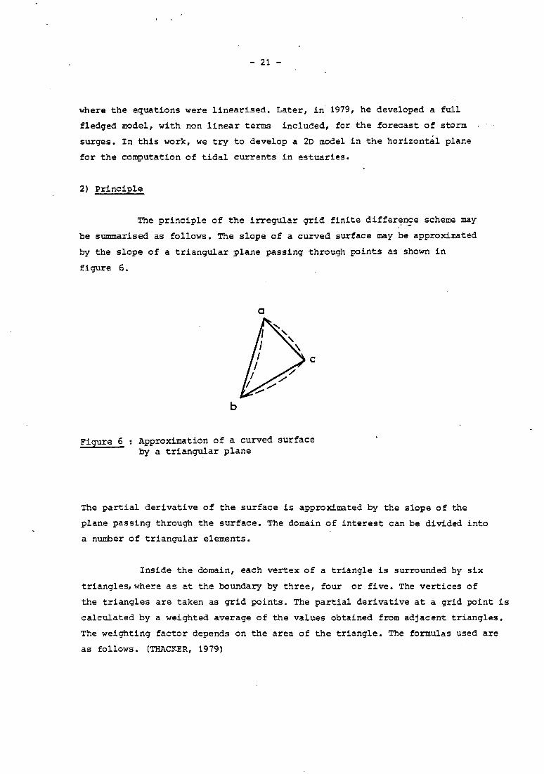
The principle of the irregular grid finite differ~n~e scheme may

be summarised as follows. The slope of a curved surface may be approximated

by the slope of a triangular plane passing through points as shown in

figure 6.

Figure 6

0

c

b

Approximation of a curved surface by a triangular plane

The partial derivative of the surface is approximated by the slope of the

plane passing through the surface. The domain of interest can be divided into

a number of triangular elements.

Inside the domain, each vertex of a triangle is surrounded by six

triangles,where as at the boundary by three, four or five. The vertices of

the triangles are taken as grid points. The partial derivative at a grid point is

calculated by a weighted average of the values obtained from adjacent triangles.

The weighting factor depends on the area of the triangle. The formulas used are

as follows. (THACKER, 1979)

- 22 -

N

!·f "' ! fi (Yi+1 - yi-1 / ô oX ·i=1

where f is iabl V any var e u, or 1;

i is the index of the grid point and N varies from 3 to 6.

3) Model eguatio~s

( 19)

(20)

The above mentioned principle of approximating the partial deriva­

tives is used in developing a numerical model in the present study. Model

equations are the equations of momentum in the x and y directions and the

equation of continuity. The equations are in the vertically integrated form.

1

au ~u ·au ar; gU (U2 + V2) Ï -+ orx+ V-- fV+ 9"r,C + 0 at a y 2 =

c El. (21)

1

av âv v!!+ ar; + qV (U2 + V2) 2 at+ uax + fU+

~ .. 0 a y c2 H

(22)

a r; ·-· + at

[23)

where the symbols have the same meaning as in the stair step boundary

madel (see page 10).

The model contains advection terms and the Coriolis term. It is to be

noted that in the present scheme, there is no direct method for approximating

the second derivatives. Accordingly, we have not introduced the viscosity term

in the momentum equations.

- 23 ...

4) Numerical resolution

The madel uses a leap frog time scheme. The equations (21) to

(23) c~n be wtitten in finite difference scheme as follows.

1 n-. 2

ui +

~t

1 1 n+t n- 1 1 v. 2 1 v. n- n- n+-]. ].

+ u 2 (av~. ·2 v. 2 ~t

+ i ax ' l.

çn~. çn +2.. a i - i (HU).n (HV)? + a y ~t a x 1 1

where i is the index of the triangl:e

5) Stability and Convergence

1

<avf:Z ay '

+

1 n+r

. gVi

= 0

1 n+r

fVi

1 n+-

fU 2 i

1 n-

(U2 2 i·

c2

= 0

+ (!I)? g ay,

1 1

+ v: n--2) 2

]. 0 =

H. l.

and n corresponds to the time step.

( 24.)

(26)

THACKER '(1978 a,b) determined the stability and convergence condi­

tions of the scheme as follows. The stability is governed by a term called

courant number given as

than 1 •

.....:..< g~h.;.;.)_ll_~.;..._~~t y = - (27)

The condition for the scheme to be stable is that y should be less

By the application ofG reen's theorem on ?n irregular grid, it is

proved that the numerical scheme is convergent as long as there is no flow across

the boundaries.

- 24 -

6) Sensibilitv of the scheme

It is to be noted that the formulas for partial derivatives

depend on the s~atial distribution of grid points. Hence, for a highly irre­

qular grid the system may ëe unstable. Sunderman (1966) introduced a factor

called numerical viscosity, which is given as follows.

f (x) = af + , 1 - a N

N

i=- 1

(28)

Where O'a'1 and fis any variable u, V orÇ. The summation is done over the

values of the variable at ehe neighbouring grid points multiplied by a.

7) Application in the Gironde

The exten.t of model domain and grid resolution is thè same as the

stair step boundary model. The whole domain consists of 1330 triangles

(fig B) In the estuarine region isoceles triangles of equal dimensions are

used with ~x = ~y =960 metres. In the region of Ile Verte, triangles of

smaller size are used. Inside the rivers, the grid is very irregular, with

~x· same as in the estuar~ne region and ~y varying according to the breadth

of the section cc;mcerned. In fact, the grid can be made more irregular than

INTE;:RIOR POINT

p[S] p

BOUNDARY POINTS

Figure 7 Types of triangles used for the application of the Gironde

Figure 8 (b) upper estuary

Figure 8 : Irregular grid used for the application of Gironde

(The shaded areas represent the islands)

- 26 -

the present one. Using bigger triangles near the seaward side, where the depths

are high, is useful in increasing the time step. ·In the present application,

the grid spacing is taken constant and it is equal to that of the stair step

boundary model. This permits to compare the pet:fo.rmance of the two models

more closely. However, in the upper estuary, the triangles are oriented in

such a way as to répresent the coastline and the islands in a better way. In

the lower estuary, such a procedure is not necessary, mainly because of the

regular geometry of the region.

Initial conditions are given as follows, The~water surface eleva­

tions are defined to be equal to the mean tide and velocities to be zero. The

model is run for more than two tidal periods, before the utilisation of the

results. The time step chosen is 30 seconds. This corresponds to about one

third of the maximum allowed time step (formula 27). In the present application,

. a time step much less than the maximum allowed value is found to give a better

solution. The value of a used is equal to 0.99. For the region of islands, the

value of a taken is 0.97. ·

All the variables u, V and ~ are calculated at the same point i.e.,

at the vertices of the triangles. Each grid point is given only one index,

ascending from the open boundary towards the head. For each grid point, a table

of values of neighbouring grid points is stored and recalled at each time step.

The neighbouring points are arranged in a counter clockwise sense. The partial

derivatives are calculated according to the formulas (19) to (20). The equa­

tions (24) to (26) can be solved for n + 1 time step, by knowing the variables

t -1 and ti t

2 a n - 2 n me s eps.

8) apen boundary conditions

The open boundary conditions at the seaward side as well as river

ends are given as in the case of the stair step boundary madel, as discussed

in page 14.

9) Lateral boundarv conditions

Lateral boundary condition states that the flow across a closed

boundary is zero. For those points situated on the closed boundary, the velo­

city variables are projected on to a line parallel to the boundary so as to

guarentee this condition. '

CHAPTER III

CIRCULATION IN THE GIRONDE

- 27 -

Introduction

This chapter deals with a brief review of the circulation studies

in the Gironde and discussion of numerical simulation results obtained from

the models applied during the course of this work. Here, the emphasis is

made on studying the lateral variations of different physical parameters and

the circulation in the region of islands. Attempt has been made to compare

the simulated results to the observed data.

The circulation in the Gironde is relatively well known, thanks

to numerous observed data available from various cruises. These cruises have

been conducted by the following organisations.

(i) Port Autonome de Bordeaux (PAB) . ·.

(ii) Institut Géologique du Bassin d'Acquitaine (IGBA)

(iii) Electricité de France (Laboratoire National d'Hydraulique)

Based on these data, various workers have studied the different

aspects of tidal propagation and circulation in the estuary. Their important

conclusions will be discussed during the course of this chapter. Numerical

modelling studies were made by DE GRANDPRE and DU PENHOAT (1978). They deve­

loped a two dimensional madel in the x-z plane to study the vertical circula­

tion in the Gironde.

In the present work, the horizontal circulation in the Gironde is

studied. The different physical parameters discussed are water surface eleva­

tion and currents. The current chapter consists of two parts, namely,

Part I dealing with the water surface elevation and Part II circulation.

- 28 -

PART I - WATER SURFACE ELEVATION

I. INTRODUCTION

The characteristics of the propagation of the tidal wave in the

Gironde estua~ are relatively well understood. This is made possible mainly

due to the availability of data from different tide gauges installed at

different places (fig 1 ) • It is to be noted that all the tide gauges,except the

one at PK 26, are placed near the south bank side. This limits the knowledge

of tidal propagation to the navigation channel, wher.~ as the phenomenon

is less understood in the other channels. However, surface elevation data

in the north bank side is available from a few cruises, which are mentioned

above. SIMMON (1979) made a prediction of different harmonie constants of

tide at different points along the abscisse of the estuary by harmonie ana­

lysis method and ether ~ethods.

II. CALIBRATION

The three models used in the present study are calibrated using

the tide gauge data. The curves of gemetrical positions of high tide and

low tide dressed by DE GRANDPRE and DU PENHOAT (1976) have also been used

for this purpose. The calibration procedure consists of adjusting the coeffi­

cients of friction at various points in the domain in such a way that the

differences between computed and observed surface elevations are minimum.

The models are calibrated from Pointe de Grave towards the head.

III. LONGITUDINAL VARIATIONS

In the Gironde, as the tidal wave advances towards the head of

the estuary, the following modifications are observed. Fig 9 (a) indicates the

geometrie positions of high tide and low tide along the abscisse of the

-estuary. It is seen that modifications in tidal range depend on the coeffi­

cient of tide. For a given coefficient of tide, when the river discharges are

high, the positions of the cürves get elevated in thë upper estuary. In all

cases, the shape of the sinusoidal curve, representing the variations of wa­

ter surface elevation with time, gets gradually deformed towards the head of

the estuary. A few tide gauges curves (fig 9 (b)) indicate the nature of the

variations of surface elevations with time along the abscisse of the estuary.

The duration of ebb increases from the Pointe de Grave towards the head.

• 1

, f • F .. I . , • 1 s . • 1 z . .. ~ . 2

0 0 z •

Fig 9(b)

POINTE Cie GRAVE

P.K. 96

•

-! . 1 r • . . • ! . .. : a

i

• 10 IZ 14 " ... '"

• $

-1 • 1

â• . • • i• • • • : a • • % • a 1

0

1 ' \ ' ' ' ' ' ', PAUILLAC

' P.K.47 ,_

0 a • ' • 10 12 14-

- V.E. ( coetf. 110 )

-- M.E. ( coeff. 45 )

:a ., BORDEAUX

P. K. 0 Figure 9(a) Tide guage curves

0

•

..

a

? ••

i 1

• • • ·10

~I.IU& • ' ry

,. "·····

··~er

V.E. , •• , .,.o ,.., . •o•·oO'

-M. M. s .... . , ••

,.., 7J·"

M.E. , ....... CMf )9 e40

Geometrical positions of high tide and low tide in the Gironde

{·After .ALI.EN, 1972 1 in CASTAING, 1981)

1

- 30 -

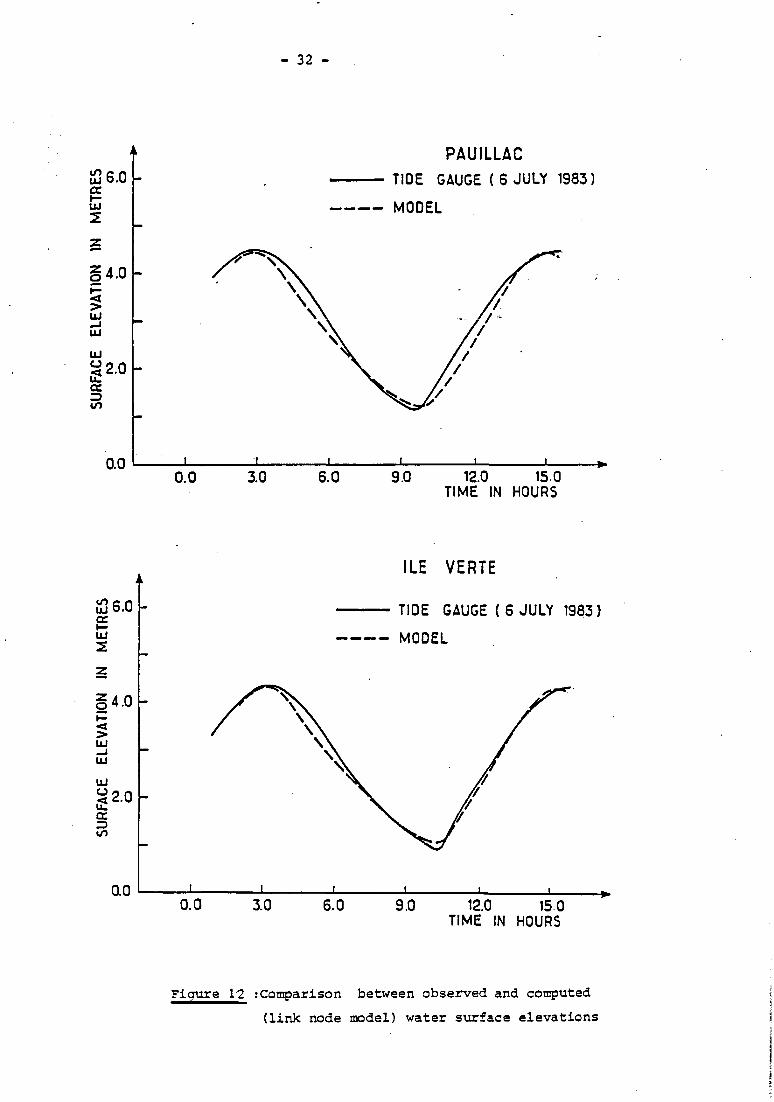
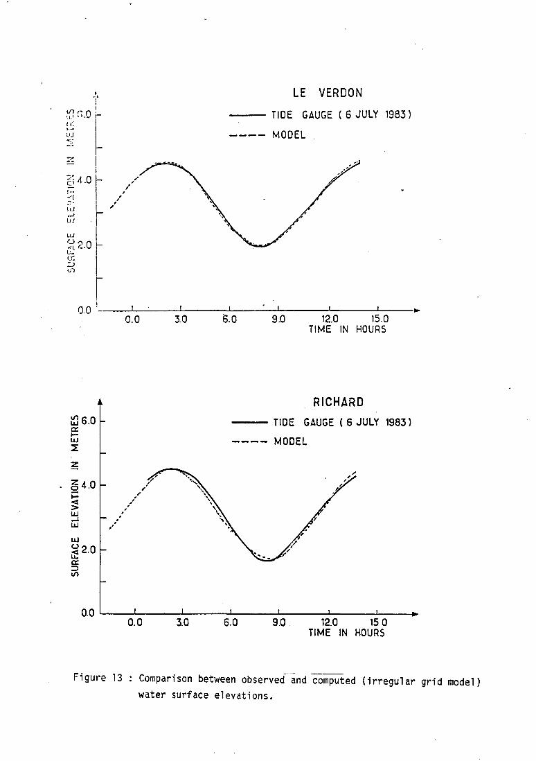
Simulation results

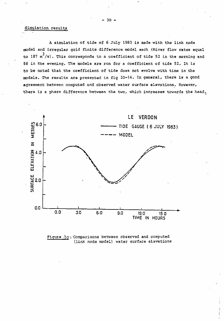
A simulation of tide of 6 July 1983 is made with the link node

model and irregular grid finite difference model each (River flow rates equal

to 187 m3 /s). This corresponds to a ·coefficient of tide 52 in the morning and

56 in the evening. The models are run for a coefficient of tide 52. It is

to be noted that the coefficient of tide does not evolve with time in the

models. The results are presented in fig 10-14. In general, there is a good

agreement between computed and observed water surface elevations. However,

there is a phase difference between the two, which increases towards the head.

§4.0 1-<t > UJ ...J UJ

UJ

~2.0 u.; a: :J Il')

LE VERDON

Tl DE GAUGE ( 6 JULY 1983)

---- MODEL

12.0 15.0 TIME IN HOURS

Figure •ÏO: ·comparisons between observed and computed (link node madel) water surface elevations

~6.0 a: 1-UJ ~

§4.0 1-

;! UJ _. UJ

UJ

~2.0 L.L.; a: ::J c.n

~6.0 ·0::

1-UJ ~

~4.0 1-~ > UJ _. UJ

UJ

~2.0 L.L.; a: ::J c.n

0.0 3.0

3.0

- 31 -

RICHARD

-- TIDE GAUGE ( 6 JULY 1983)

---- MODEL, ,

6.0 9.0 12.0 15.0 TIME IN HOURS

LA MENA

--- TIOE GAUGE ( 6 JULY 1983)

---- MOOEL

'/ v

9.0

'/ '/

'1 '/

'/'/

12.0 15.0 TIME IN HOURS

Figure 11 Comparison. between observed and computed (link node model) water surface elevations

:il 6.0 0: t;j ~

a4.a ~ > UJ ...J UJ

UJ

~2.0 u:; c: ~ lof)

::a 6.0 c: ..... UJ ~

à4.0 ~ ~ > UJ ...J UJ

UJ

~2.0 u:; a: ~

"'

- 32 -

PAUILLAC -- TIOE GAUGE ( 6 JULY 1983)

---- MODEL

0.0 3.0 6.0 9.0 12.0 15.0 TIME IN HOURS

ILE VERTE

-- TIOE GAUGE ( 6 JULY 1983)

---- MODEL

0.0 3.0 6.0 9.0 12.0 15.0 TIME IN HOURS

Figure 12 :Comparison between observed and computed

(link node model) water surface elevations

• 'i' j

cf),~ n! i';~ .~ .... ~ r-•·-:.•J ~··

=-= 1 i

~~tt .0 ~ ~:i 1 ~~ 1 • ..J r-liJ . 1

~2.0 ~ ~ 1 UJ

r

1 , , ,

1

,. ;'

'

LE VERDON

-- Tl DE GAUGE ( 6 JULY 1983)

---- MODEL

·.'-../ .

.· ,•

0.0 i _ ___t__: _ ___J __ --:-L,__---=~-----=-=--=--~~--12.0 15.0 0.0 3.0

~6.0 0:: 1-UJ ~

~4.0 1-

~ UJ ...J UJ •'

. .

TIME IN HOURS

RICHARD

-- TIOE GAUGE ( 6 JULY 1983)

---- MOOEL

o.o L__o_L.o __ _l3.o __ ---.J6.L....o---9.1..-.o----:,~2.-=-o--=,s:-:o~_. TIME IN HOURS

Figure 13 Comparison between observed and computed (irregular grid model) water surface elevations.

~6.0 0:: w ~

UJ

;:12.0 u.; 0: :::> 1,()

~6.0 0: ..... UJ ~

à4.0 ..... <X > I.&J ..J UJ

UJ

;:12.0 u.: 0: :::> 1,()

0.0

, 1

1

1

/

1 , 1 ,

0.0

1 1

1

/

, 1

3.0

3.0

LA MENA

--- TIOE GAUGE ( 6 JULY 1983)

---- MOOEL

6.0 9.0 12.0 15.0 TIME IN HOURS

PAUILLAC -- TIOE GAUGE ( 6 JULY 1983)

---- MOOEL

6.0 9.0 12.0 15.0 TlME IN HOURS

Fiqure 14 Comparison between observed and computed (irregular grid finite difference model) water surface elevations

- 35 -

IV. LATERAL VARIATIONS

The transversal variations of tidal propagation are mainly

due to the depth variations across the section. The lateral differences also

occur due to meandering effects, presence of islands, sand banks etc. In fact,

these small lateral differences in phase speed of tidal wave gen~rate trans­

versal currents.

In shallow water, the tide propagates with a velocity, which is

approximately equa1 to .{:;:"(in the absence of friction), where h is the

depth. Thus in deep channels, the tide propagates fast (further if friction

is taken into account, the deeper regions are subjected to less bottom

friction than shallow regions) • The tidal wave propagates with lateral varia­

tions due to the presence of islands, sand banks etc.

Since the data from tide gauges is available only at the southern

bank side, comparison of transversal differences of surface elevation between

two bank sides is not always possible. In a study of lateral differences in

tidal propagation, TESSON GILET (1981) compared the observed surface elevation

data with calculations done by the author herself by an interpolation of tide

gauge data. The results showed much difference between the observed and compu­

ted values. The calculations seem to be susceptible to errors and the results

are not reliable.

--.... -.... ~ .. ~ \

.. -t•·

,. ' ~0 ',

r \ \ \

1 1 \ 1 \ \ \

' \ ' \

'

':/lf>'c:orcl..,con 1 \ \ '.

\

' \ \

Figure 14

;;,~ i.;.---

co tidal lines in lower estuary

·- 36 -

Fig 15 represents the cotidal lines for lower estuary. It can be

seen that the tide propagates in advance in the Saintonge channel. From

Mortagne (PK 74), onwards the phase differences between two banks are absent.

·At Pauillac, the observations (ALLEN, 1972) show that the tidal wave propaga­

tes faster in the navigation channel.

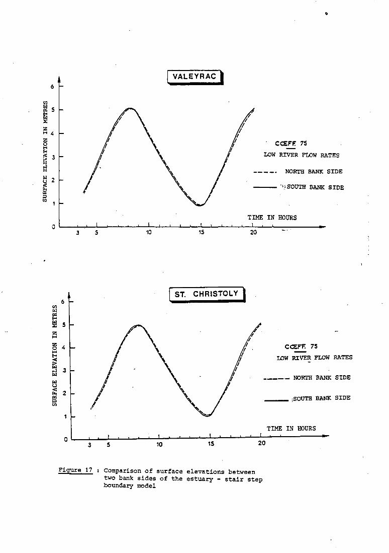
Simulation results

Stair step boundary model results presented in fig. 16 to-18 show

that at Richard, Valeyrac and St. Christoly, the phase differences between the

two bank sides is more along the southern side and these differences increase

gradually towards the head. It is to be noted that the compa;ison is made along

the'y direction.of the model domain,

6

Cil

fiJ 5 tl ::E:

z 4 1-1

z 0 1-1 E-4 s: r:w

3

...::1 r:w r:w 2

~ ::;l Cil

0 3

Fiaure 16

RICHARD 1

cœ:FF. 75

LOW RIVER FLOW RATES

--- - NORTH EANK SIDE

s 10 15 20

Comparison of surface elevations between two bank sides of the~stuary - stair step boundary model

SOUTH EANK SIDE

TIME IN HOURS

0 3 5

6 en CzJ Ile: .... ~ 5 z 1-1

z

" 0 1-1 .... ~ CzJ

3 ...:1 CzJ

CzJ u < ~ Ile: ::J en

Figure 17

'1 '1

'1 '1

'1

VALEYRAC 1

'1 '/

'/ '/

'1 '1

JI' '1

0

CCEFF. 75

LOW RIVER FLOW RZ\.TES

NORTH BANK SIDE

--- ''.•SOUTH BANK SIDE

TIME IN HOURS

10 15 20

ST. CHRISTOL Y 1

'1 '1

'/ '/

'/ '1

'1 '/

'1 '/

Comparison of surface elevations between two bank sidas of the estuary - stair step boundary modal

CŒFF. 75

LOW RIVER FLOW RATES

----NORTH BANK SIDE

------ 1soUTB BANK SIDE

TIME IN HOURS

rn ~ tl ::t

:z .... s .... ~ ::> [:IJ o-1 r:a r:a u

~ :J rn

rn ~ tl ::t z ....

a .... ~ &i

-,, o-1 r:a r:a u

~ :J rn

•

PAUILLAC., 6

5

~ C:Œff. 7S

LOW RIVER FLOW RATES 3 ~.

---- NOEmi BANK SIDE

2 SOUTH BANK SIDE

1

TIME IN HOURS

0 3 5 10 1S 20

ILE VERTE 1 6

5

~

CCEFF. 75

LOW RIVER FLOW RATES

---- NOR'l'H BANK SIDE

SOUTH BANK SIDE

TIME IN HOURS

0 3 5 10 15 20

Figure 18 Comparison of surface elevations between two bank sides of the estuary (stair step boundary madel) .

e.a

en rz:l c:z::

tl ::E :z: 1-4 4-.a :z: 0 1-4

~ > rz:l fj rz:l t.a t.J < r:. c:z:: ;::) Cil

a.'

e.a Cil ra ~ E-t ra :t

z .... 4.0

z 0 .... E-t ~ > ra ~ ra LO

ra CJ ~ r.. ~ 0 Cil

a. •

Figure 19

LOW RIVER FLOW RATES COEF 75

\ -NORTH BANK S IDE

_ SOtrrH BANK SIDE

.. ... ... .. - TIME IN HOURS

RICHARD

LOW RIVER FLOW RATES

COEF 75

-NORTH B~NK SIDE

SOUTH BANK SIDE

' ... ... ... .. - !IME ·IN HOURS

VALEYRAC

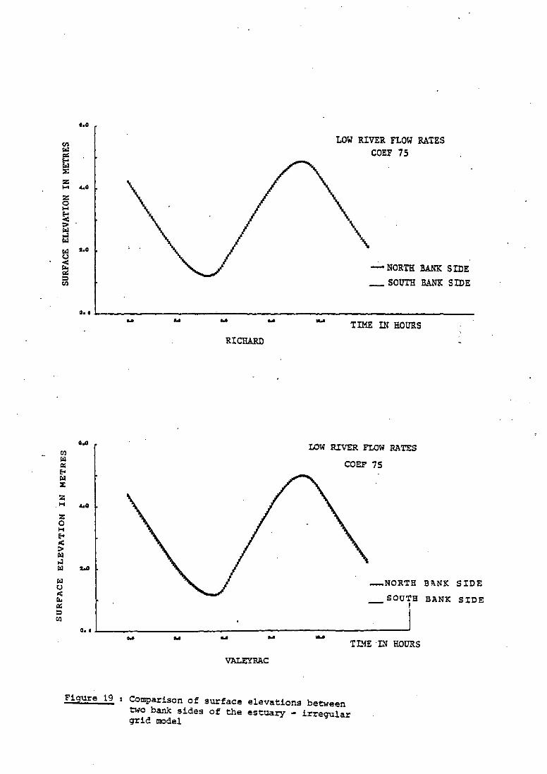
Comparison of surface elevations between two bank sides of the estuary - irregular grid model

tl) loO ~ Il:: E-< ~ ::t

::z: 1-4

::z: .&.0

0 1-4 E-< < > ~ ..:l ~

LO ~ u < "" Il:: c ~

o. 1

tl)

l%l Il:: E-< l%l ::t

::z: 1-4

.&.0

::z: 0 1-4 E-< < ::> l%l ..:l l%l LO

l%l u < "" Il:: c tl)

o. 1

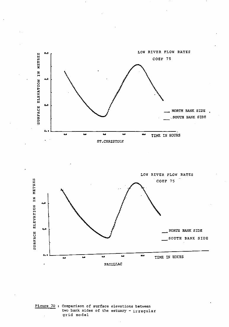
Fiqure 20

LOW RIVER FLOW RATES

COEF 75

- NORTH BANK SIDE

., SOUTH BANK SIDE

... .. ... .. - TIME IN HOURS

ST.CHRISTOLY

LOW RIVER FLOW RATES

COEF 75

NORTH BANK SIDE

SOUTH BANK SIDE

... .. - TIME IN HOURS ... .. PAUILLAC

Comparison of surface elevations between two bank sides of the estuary - irregular grid model

.

~ L&J 0::: 1-- .5 L&J ::E:

z -z 0 4 -1--< > L&J -' L&J '3 L&J u < u.. c::: :::1 ~

a

1 1

~ L&J 0::: 5 1--L&J ::E:

z -z 4-0 -1--< > L&J -' 3 L&J

L&J u < u.. 0::: ::::l ~

COEF 70

't+t+t N:lRTB BANK SIDE

SOO'l'B BANK SIDE

~

3. 4-

Il

TIME IN HOURS 13

Figure 21(a) Comparison of surface elevations between two bank si des

of the· estuary (link node model)

COEF 70

E.

s ~

3 l.

1 13

1 lJ

TIME IN HOURS

a 3 4- 5' G

GRAVE RICHARD LAMENA ST.CHRISTOLY PAUILLAC ILE VERTE

Figure 2l(b), Surface elevations along the axis of the estuary during high river discharges (link node model)

- 42 -

It means that in the region of regular geometry of the estuary,

the tidal wave accelerates in the deeper region i.e., along the navigation cha­

nnel, which is situated near the south bank side. Co tidal lines (fig. 15)

indicate that the tidal wave enters into the estuary with a slight advance

along the north bank side and the phase differences between the two bank

sides are absent from Mortagne onwards. Upstream, from the middle region of

the estuary, there is no data regarding the tidal variations along the north

bank side. At Pauillac, the simulated curve of surface elevations indicates

that the tidal wave is in advance along the north bank side. It is to be noted

that along the lateral section considered for comparison at Pauillac, the dis­

tance travelled by the tidal wave is less at the north bank side than at the

southern side. However, observations (page 36) show that the tidal wave moves

faster in the navigation channel at Pauillac. Upstream, at Ile Verte, the

lateral differences in phase speed between two bank sides are absent, as

the width of the estuary reduces considerably towards the head.

A comparison of surface elevations between two bank sides is made

using irregular grid finite difference model, (fig. 19-20). The lateral diffe­

rence are less significant in these results so as to make comparisons between

the two bank sides.

Fig. 21 (a) indicates that small lateral variations in surface

elevation are p~actically absent in the link node model. This explains the fact

that this type of model cannot fully describe two dimensional aspects of the

fLow.

Fig. 21 (b) represents the surface elevation curves as a function

of time along the abscisse of the Gironde during high river flow rates (1300 m3/s).

For those points in the upper estuary, these curves get shifted upwards com-

pared to fig. 21 (a), though there is not much change in tidal ranges •

•

- 43 -

PART II - CIRCULATION

I. INTRODUCTION

The French estuaries such as the Seine, Loire and the Gironde

are caracterised by high tidal ranges. In these estuaries, the dynamics is

controlled by the action of tide. The currents produced by density gradients,

which are observed in the estuaries of certain other continents, for example,

Vellar estuary (India), are negligible. In fact, in the case of the Gironde,

DU PENHOAT and SALOMON (1979) proved that the effect of introducing a

density gradient in their 2D model in the vertical plane (X-Z) made little

influence on the current patterns. In the present study, the models do not

take into account of the density gradient currents.

Since the Gironde is a hypersynchronous estuary (ALLEN and SA~MON~

1983), in general, the intensities of currents increase from the mouth towards

the head. Variations of velocities in different lateral sections are determined

by the topographical variations. Generally, maximum currents are observed in

deep regions. Modifications in circulation patterns are caused due to meandering

effects, presence of islands, sand banks etc.

II. BRIEF REVIEW OF CIRCULATION STUDIES IN THE GIRONDE

Various workers have described the circulation patterns in the

Gironde. Here, only a few of them will be mentioned. ALLEN (1972) deduced

the circulation patterns in the estuary based on the data between 1965 and

1972. He described the main features of longitudinal and lateral variations

of currents. Some of his conclusions may be summarised as follows. At PK 93

and PK 89 maximum flood currents are observed in the Saintonge channel. However,

at PK 89,. the bottom flood currents are found to be maximum in the navigation

channel. This is explained due to the curvature of the Pointe de Grave which

directs the flood currents towards the northern channel. Further upstream,

upto Pauillac (PK 47) both.flood and ebb currents are found to be maximum in

the navigation channel. Between PK 41 to PK 35, the ebb currents are of same

intensity in navigation and Blaye channel, during spring tide and mean river

flow rates. In the same region, during the same conditions, flood currents

are found to be stronger in the navigation channel at PK 35.

- 44 -

TESSON GILET (1981) made a study of lateral variations of velocity

maximum along a few lateral sections. These informations are synthe~sed for

a coefficient of tide equal to 80 and slightly above. The river discharge rates 3 -1 are 1000-1500 m sec • At PK 89, intensity maximum of flood currents occur in

the Saintonge channel, where as ebb is stronger in navigation channel. At PK 71,

the lateral variations are less with slightly higher values found in navigation

channel. Along this lateral section, surface ebb currents are stronger towards

the right of the dike of Valeyrac, which is due to the presence of the dike.

At PK 52, during flood, the velocities aie found t~~e maximum in the median

channel, whereas the ebb currents have their maximum lntensities in the navi­

gation channel • Accordingly, median channel is referred to flood channel at PK 52.

Figure 22

FLOOD

EBB

__ Vitess.e ma:d.,.;a,l.a. c!u courant (1 cm • 1 m/s) · S~&ce -

J'on4 -- • Lieu c!u ~ cie courant c!&ns 1& section

S~&ce • J'on4 · .lfo

t4cère c!•viation c!es.masses c!'eau S~ace ~ J'one! 7if

Observed velocity maximum along a few lateral sections of the Gironde (After TESSON GILET,1981)

CASTAING (1981) gave much additional informations to ALLEN's work

on circulation. This includes a study of the influence of river discharges

on currents. Fig 23 gives an example indicating that the intensities of sur­

face currents during ebb are considerably increased, when discharges are high.

However, at the bottom, there is not much change in the magnitude of currents.

- 45 -

1.5 Q-150 m 5 s 1.5 ,.,_ 1 ,,\

• 1 \ ; ....... _, \ 0.5 • 1 1

1 0 0

,,..'. h

_o.:s \\ /1 -0.5

-1 ' •' -1 ' , ., -1.5

'0 -1.5

-2 -2

-2.5 -2.5

,.-, /. ,, .

1 ' \ 1 \ 1 ' . ~ '

, . '\ Flot

.\\ // -, 1 Jusant \./

•

\) -:--- surface .. •----- 1 m 1 fond - bottom

Figure 23 : Variation of velocity due to an in the navigation channel at PK

increase in river discharges 89(After CASTAING,1981)"

AMONT

Figure 24

1 Sens de motion des direc:tiOM ou C:OUI"' du flot - du jusant.

w ---= . -r

Hydrological exchanges between different channels (After CREMER, 1975)

... ,

AVAL

-----

CREMER (1975) and CASTAING (1981) studied the significance of

transverse currents.in certain regions of the estuary (Fig 24). For example,

near PK 49, the currents are parallel to the axis of median channel. Near

PK 56, the ebb currents tend.to move towards the north bank side. At stations

3 and 4 (PK 62), the currents are found to be parallel to the sand bank i~

the beginning of flood and later become more inclined, where fs at station 5,

flood currents are parallel to the bank.

- 46 -

Laboratoire National d'Hydraulique (L.N.H,) made various studies on

the circulation and hydrology of the Gironde. Besides numerous in situ measu­

rements, these studies include mathematical modelling and hydraulic modelling.

Two of the hydraulic models developed are (Rapport n° 32 - 1975 and n° 17 -

1971 : personal communications) the one developed for the region between ·

Pointe de Grave and St. Christoly and the· ether for the region between St.

Christoly and Bec d'AJn.bes. Based on tidal variations and salinity (at the sea­

ward side) at the left h and side of the boundary and river discharge rates at

the right hand side, the current pattern in the domain was simulated, The re­

sults are presented in the form of instantaneous current vector diagrams for

every one hour during a tidal period together with a few comparisons with

observed currents at the surface. A few of these results will be discussed

later in this chapter in relation to a comparison with simulation results

obtained during the present study.

The current measurements made by L.N.H. give a few additional de­

tails to the circulation in the estuary described above. The surface current

charts for the lower estuary show the predominance of flood in the northern

channel between Pointe de Grave and Talmont (PK 85). However, ebb currents are

found tc be slightly more intense in the navigation channel than those in the nor-

them channel in this region. Near Lamena, at PK 64, a few measurements across

the section show that flood currents are stronger towards the north bank side,

where as duriog ebb, currents are of maximum intensities in the navigation cha­

nnel in that section. The current measurements also show the presence of an

eddy between PK 67 and PK 65 during the slack from ebb to flood.

In the upper estuary, observed data across a few lateral sections

reveals the following features.

(i) At PK 54, there is a sharp gradient of axial velocities across the navi­

gation channel during flood and ebb, with higher values found towards the south

bank side,

(ii) At PK 50, high intensities of currents are observed very near the south

bank side.

(iii) At PK 38, the surface currents have almost same magnitudes in the navi­

gation channel and the Blaye channel, with slightly higher values found in

the former than in the latter during flood and vice versa, during ebb.

The hydraulic madel simulations show a relatively good agreement

between simulated currents and observed currents. In the madel of St. Christoly,

at Grave, flood starts five hours before high tide and lasts until two hours

- 47 -

after high tide. Three transient eddies are present in the current field. They

are found near PK 92, PK 83 and PK 66. Sufficient observed data is not availa­

ble to verify this point; except for the one present at PK 66

The hydraulic modal developed for the region of islands shows the

following aspects. Flood currents start at four hours before high tide and

continue upto the hour of high tide at Pauillac. Slack of flood occurs one

hour after the high tide at Pauillac: The düra~ion of ebb is in between one

hour after high tide at Pauillac and four hours before high tide. The slack

of ebb is produced slightly in advance than in nature.

III. DISCUSSION OF SIMULATION RESULTS

Numerical experiments are done with the stair step boundary model

and the irregular grid finite difference mcdel for a coefficient of tide 75 3

and low river discharge rates (183 m /s for both the Dordogne and Garonne

combined) • The results are presented in Appendix I - III. A simulation of tide of·~·­

coefficient 70 and for the same discharge rates, as mentioned above, is made

with the link node model. The computed currents are presented at every one

hour.

1) Stair step boundary modal

The general features of circulation may be described as follows

(Appe~dix I) • In the lower estuary, the currents flow parallel to the coast

with intensities decreasing from the centre towards either coast. This pattern

continues upto PK 60. Between PK 85 - 90, the ebb currents are found to be

intense in Saintonge channel. During slack, a few transient eddies are present

in the current field, a prominent one being observed between Valeyrac and

St. Christoly. Their lifetime is about one hour. During the transition from

ebb to flood.J the eddies are clockwise and vice versa. These transient eddies

get dissipated due to bottom friction and viscosity.

Between PK 60 and PK 50, flood currents are very small in intensi­

ties near both the bank sides, though navigation channel has high depths in

this region. This is probably due to the fact that the navigation channel is

situated very near the coast in this region and any possible poor representa­

tion of the coast can affect the computed values of currents. During ebb, the

currents are equally intense in this channel as those found at the central

region. This confirms the fact that navigation channel is an ebb channel in

this zone.

- 48 -

In the region of islands, the notable features are as follows.

Between Pauillac and the island of Philippe, flood currents are strong near

the north bank side. U~stream, between PK 41 and PK 35, flood is more predo­

minant in the navigation channel. In the Blaye channel, along the same longi­

tudinal distance, beth flood and ebb currents are fo~d tc be less in magnitude

than those of navigation channel. Ouring ebb, all along the upper estuary,

maximum intensities of currents in different lateral sections are found in

the navigation channel

2) Irregular qrid finite difference model

The computed currents are shown in aooendix II • It is tc be

recalled that this model has the same topography and open boundary conditions

as the stair step boundary moael. Accordingly, the discussion of the results

is made in comparison with those obtained in the previous model.

The current field in the region between the Pointe de Grave and

seaward boundary is different from the one obtained from the stair step boun­

dary_model. Considering the fact that the calipration is done from the Pointe

de Grave towards the head of the estuary, this aspect is not discussed here.

In the lower estuary, the computed currents are very much similar

and comparable to those values obtained from the previous model. In the diffe­

rent lateral sections, the velocity gradients are less marked and currents

near the coast are less feeble than those found in the previous model. A .

transient eddy is present at the same location as the previous model, i.e.,

between Valeyrac and St. Christoly. In this model, the eddy dissipation

is only by bottom friction, viscosity being absent.

In the upper estuary, the grid configuration near the coast is

different from the previous madel. Between Pauillac and St. Christoly, the

ebb currents are represented in a better way than the previous madel.

Again, lateral differences are less visible in this region. At PK 50, ebb

is the strongest in the navigation channel between the island of Trompeloup

and left bank side in that section. It is re~alled that in the stair step

boundary madel, high intensities in ebb are observed in the passage between

the islands of Trompeloup and Philippe. Considering the high depths of the

navigation channel in this region, the results obtained from this madel seem

to be more reliable.

In this madel, lateral differences in the computed parameters are

less present compared to the stair step boundary madel. This may be attributed

to the effect of the procedure of smoothing (equation 28). For the present

- 49 -

simulations, a small value of the smoothing factor of the order of o.ol

(corresponds to a = 0.99 in the equation 28) is found to be necessary tc

guarantee numerical stability. This procedure does not have much physical si­

gnificance and it is found to be necessary because of the difficulties in

introducing the viscosity term in the madel.

In the region of islands, the comp~ted currents are not much pre­

cise. It may be necessary to choose smaller triangles than those used tc impro­

ve this point. The circulation in this region, based on this model, is not

included in the discussions.

3) Link node model

The computed currents are shown in (Appendix III) , the simulation

being made for a coefficient of tide 70 and low.discharge rates (189 m3/s for

beth the Dordogne and Garonne combined). As discussed earlier in page 42, in this

madel the tidal wave ·propagates without any significant phase difference in

the lateral. Moreover, since the centrifugal forceis absent, the phenomenon

caused by meandering cannet be reproduced by this mo~el. Lateral and longitu­

ainal variations in velocities are determined uniquely by the depth variations.

A few of the salient features can be mentioned as follows. Near

PK 90, beth flood and ebb currents are found to be of maximum intensity in

the Saintonge channel : upstream, maximum currents are observed in the navi­

gation channel in the lower estuary. In the upper estuary, between PK 35 to

PK 45, the currents in Blaye channel are slightly more intense than those va­

lues found in navigation channel. This is in accordance with the observations

(page, 43) and a significant improvement from the ether two models.

Small transversal currents are present at certain regions and du­

ring certain stages of tidal propagation. These currents are present due to

the grid configuration. Their significance lies in the fact that they are pre­

sent only during slack. These transversal currents are, probably, comparable

to the presence of transient eddies in a 2D model. Tc indicate a few examples,

during ebb, feeble lateral currents flow downward from the bank of Plessac

at PK 35 ~owards the navigation channel. In the lower estu~ry, between PK 80

and PK 85, lateral currents towards the north bank side are present. Downstream,

near Verdon, feeble currents flow towards t~e southern side. During flood, the

direction of transverse currents is opposite tc those of ebb.

- 50 -

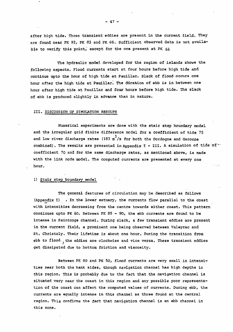
4) Trajectories

The simulated current field can be used ta compute the trajectory

of a water particle at different points in the domain. This allows ta deter­

mine two lagrangian parameters, namely, the displacement made by a water par­

ticle and the residual displacement during one tidal period. The former

parameter willbe discussed here and the latter during the V chapter. The cal­

culation is done as follows.

t X (t) = ]

0 U(x,t) dt + X 0

where X0 is the starting point, U, the velocity and x is the co-ordinate of

the point of arrival.

COEF 70 Tl!AJECTORIES Pl::98

MEAN RIVER FLOW RATES

Figure 25

h"""'~ 1 l"' LE VE CON

PTE AUX !SEAUX

D"""" " S'l'AR'l'ING POINT

ARRIVING POINT

Computed trajectories of water particles at a few points in the lower estuary (stair step boundary madel) •

- 51-

The calculation·is done using the stair step boundary model,

the integration being carried out over an interval of time equal to 6 minutes.

A few examples of results are presented in fig 25 to 27. In figure 25, èonsider

two particles of water starting at PK 85, one travelling through the navigation

channel and the second through the Saintonge channel. It can be seen that the

displacement of the particle is more in the northern·channel. This shows the

predominance of flood and ebb near the north bank side in this region.

Upstream, betwcen PK 78 and PK 62, during flood as well as ebb,

displacements are maximum for the trajectroies of particles near the centre

(fig. 26). In this region, velocities are the strongest at the centre with

intensities decreasing towards either coast, as may be observed in current

vector diagrams.

A few trajectories drawn for. upper estuary are shown in figure 27.

Let us consider the particles starting at PK 54 and PK 52 travelling downstream.

It is seen that the displacements are maximum for those passing through the

centre and the navigation· channel. During ebb, the displacement is maximum

in the navigation channel, showing the importance of this channel in this

region in canalysing ebb currents.

Between Bec d'Ambes and Pauillac, the computed trajectories have

displacements slightly higher in the navigation channel than in the Blaye cha­

nnel.

A few trajectories are dra'm from the current field obtained from 3 a simulation made for high river flow rates (1300 m /s). In the upper estuary

(fig 27), the displacements of water particles are maximum in the navigation

channel. Moreover, these increases in displacements are more pronounced during

ebb.

A few informations about the observed trajectories are available

in the form of displacements obtained by the release of drifting peles. These

give the displace~ents along a column of water. CASTAING (1981) computed a

few trajectories based on the observed residual currents using a method pro­

posed by SIMMONS ( 1966). These results are supplemented wirh a few data obtained

from the release of drifting peles and are presented in figure 28· The trajec­

tories are outside the model domain or very near to the seaward boundary

so as to make comparisons with the computed trajectories. Also, a few release

!'0:78 J '"T Pt_4

.....----: ~ ~

...... -_,=-

--1

1 ST .CH?.!S!~!..'!

1

,. J VALEYRAC

POINT OE AICHARO COEF 75

LOW RIVER .:FLOW RA 'l'ES

TRAJECO'l'RIES

-- lo371 KH

. STARTING POINT

. ARRIVING POINl'

- -- -

"'<78 1 ""r P~4

____. ~1 - . ~ 1

1

1

::::---

1 ST ,CHRISTOLY 1

1 VALEYRAC

P!JINT OE R!CHARO COEF 75

High river flow rates

TRAJECTORIES

!o371 '<H

STARTING POINl'

ARRIVING POINl'

Fiqure 26 Computed trajectories of water particles at a few points in the middle part of the Gironde

STARTING POINT

ARIUVING POINT

• STARTING POINT

ARRIVING POINT;: .

Figure 27

COEF 75

-- lo371 KM

COEF 75 TRAJEC'l'ORIES

A - ILE PHILIPS

B - ILE PATIRAS

C - ILE NOUVELLE

HIGB RIVER FLOW RATES

-- 1.371 KM

A - ILE PHILIPS

B - ILE PATIRAS

ILE NOUVELLE

ILE VERTE

ë.omputed trajectori es in the upper estuary

- 54 -

of drifting peles were made by Laboratoire. Municipal de Bordeaux in 1962

and 1970 in the region of Bordeaux. For the estuarine region, much data is not

available for comparing with the computed trajectories from the stair step boun­

dary model.

Figure- 28

N

ô 0 4km . .._. __ __

• 3

+3 Flot

Jusant

Trajectories of cuxrents during spring tide (after CASTAING, 1981).

COMPARISONS WITH OBSERVATIONS

The simulation results obtained from the different numerical models

are compared with the measurements and simulation results obtained from the

hydraulic models developed by the L.N.H. (page 46). The ccmp.arisons show that

the 2 D models reproduce well the hours at which slack occurs and the presence

- 55 -

of transient eddies during slack. In the hydraulic model of st. Christoly,

the transient eddies are located in the principal channel. In the case of

numerical models, the width of the estuary is found to determine the size

of eddies. The link node model also reproduces well the hour of slack.

A few of the differences found with reference to the L.N.H.· results

may be mentioned as follows. In the case of stair step boundary model, the

computed values of currents near the south bank side between PK 50 - 60 are

found to be very small, in spite of the presence of the principal channel. This

is explained (page 47) due to the representation of the coast by a stair step

boundary in this region. The current measurements in the navigation channel

at PK 50 by L.N.H. (Rapport no 17) show that the magnitude of surface currents

are of the order of 2 rn/sec, during spring tide. Upstream, at PK 38, the

computed currents in the Blaye channel are found to have less magnitudes than

those in the navigation channel, in the case of beth the 20 models. Observa­

tions show that the magnitudes of currents in these two channels are comparable.

This aspect is reproduced only in the case of the link node model. This illus­

trates that the flexibility of the link node model is useful in describing

the circulation around the islands.

The computed currents obtained from the different models are

compared with observations at a few points in the estuary. The measured currents

(MOYES, 1975), exist at the surface, mid depths and bottom. During the period

of measurements, the river discharge rates were 600 m3/sec. for both the.·rivers

together. Figure 29, gives observed values at a few stations. The depth averaged

currents obtained from different models are compare~ with these observed

currents at mid depths (see figure 29) • 1o

It can be seen that the stair step boundary model is giving the

maximum precision. The irregular grid modal is also sufficiently precise

in the comparison~. The link node model resulta show that the magnitudes of

computed currents are less than those of observed. In this model, for a

given polygon, the flux of water occurs through various sides of the polygon,

whose dimensions are not the same. So the velocities obtainad may not be

compared with 9bserved velocities.

11 ·Fig. 30 shows observed currents at two stations near the south bank

side of PK 86. The first station is situated at zero metre isobath and the

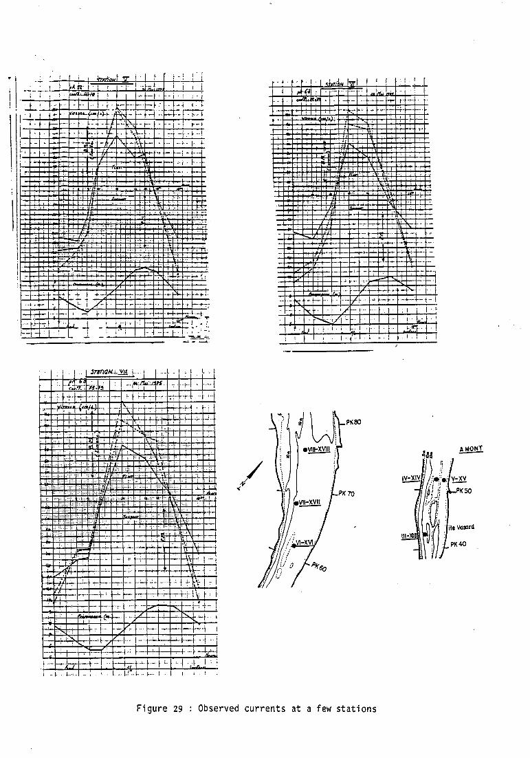
: ': 1 ii~, .. , v!· i lJ . .. ~ ; ) A.k· i·. 1 ;· -~- 1 ·- -... J. 1 j

--------·~Fr~~-~--... .;...+--'--+-..2!-ll~Z+---l--l--+ : : : 1 ,.wa.~-""•MJ : 1-~ -r· :·i · '·;

:..L.! -~- .. f . ; . r- ·---·=+ .. -+-i 1 .•

, . , • , ... .. ........... (·H ~~~ -~- , + ... :r~p::.-r:-r--r 11- -1-·- ···t·f-+-·1 ,:,;"-; ·f-··f· .,. ~-· 1 ! ' ! . - . .. 1-::-~ -~ ' ~ '·.i\.:- --! -! - f . ! i . - ' ~~-- ~ -1-.f~•+-li-·/· .:-.., --•\t ... -+· 1· ~-i.". . 1"' C.,...f-+-·! -i---l i.

':-· -~- ··i·l-·­

·- l-

'Il:.· ''.

1 r.- -',

1

i i

' 1

1- : ;- !-..-. t-" '.

1-'-!-

: ; . J 1 JriTJQN..i.~ j .... 1 .. i ' 1 ' i

1· ' .. ;.. . ·"-----;-.. ""!'" .... - .... ".. •· . , . .1.. ...... . ,. --:·: ....... c.. . . .. i· ' ... .. , .. ~:cr.:~:u" <•,.JtJ ...... \.· ... r-· ··:· -r r-· ·+···1 f .. :.

H-+-1--+ .. H-+1-+-'.. ·-+j .;r~- + ~- ; :!-- · !- '"' ·- ...

• 1 1

. ; •.. 1.

... i

--·!'·. . 1

"1 ..... --1

• ~- f +- .. ·f- '·

' . i::

;: :); ., .•·" .. ;\ ' l ... i....

. ,.. l'' . • ~ .. ,.: f,. ..

'"'' .. ,, ... ' ...... ~±--' .. ' : ,, ·:·:; ~~ .. !'!r+ ..

,., ......... ~r--~r--.. ·lt'· '"ï

,:;: .. ..: i

.. ' ' ................ "" -..... :~ ·\-+--·-.. 1

---1 " .... , .... - + -·-\\ ... , 1 .: .. :

., ... '". : ... ;. 1-r-- ~t- -+~r·! . ·! -i4=:-+f:~, ' .• :.. .. ~ ':''" --' ....... ... .. . .. - - -· ...... ' ,;, ·! j .. ' '-.:- ! ' ! ~~·-·-.;. ........... ; ... i.. -· ~- ·;- .. .,.. ..• ,.[\ ~'

t--+'...;'-+-·'--1'--+· --·· ·~· .. t'' ••••. --· 7 --rç· ···-+···~ +·-: !

" +--'1·7 ... , ..... 1..... r-;--'-·· ··· -·i .... :.

i .. j ••. 1 ... • ... ~- •• ~- .... j .... ~ .... 1

/ <

r . . f • . 1 . jlf '·4 1 .... ~ I!H. - ' . : l 1

-rr-r .... -:-· .; ' . .... ~- .,.:f'+-...-···-··

·-~ +- ~

-r

·f · · r- ···· -~ ... ! · -.:.1 -·1- ...;.... - t-:-!f'- __ ,__!- "ël~tT ~- ·~r-· ... ~--.

- ~~ -r- .;..~- ··-+ -· -·r- .... - -'-·!-'-·· • + ···--

-- - ~"';:· - - · · r --f.f ·· 1~

. r-- .... v' . ''J . ! ' 1 ' ' ' lU.ë 1 ' .. ' 1 .. > .

1 .. --1' 1 •.

PKSO

't '

·--·~ i i

j· 1

! ' ~

1' '. .. :l' j

1.! i

Figure 29 Observed currents at a few stations

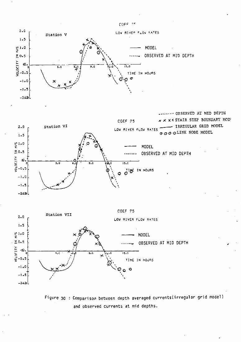
2.G Station v

~ 1.0 r

! 0.5

>-: a;J. L----------- ---u 0 0

~ -0.5 >

-1.0

-1.5

-2-ill

2.0

1.5

!C l. 0 x: ~ 0.5

>­

3.0

Station VI

' ' 0 •, ' ' ~

' -----·

--~- ---- ___ __. ··.o • !5.o

MO DEL

OBSERVED AT MID DEPTH

\ '. ')(\. \ TlME lN HOURS

\\ (!)\~ Q

' ' ' '

COEF 75

••..•.. ··· OBSERVED AT MID DEPTH

x x )( l( STAIR STEP BOUNDAF.Y MODï

------ IRREGULAR GRID MODEL LOW RlVER FLOW RATES

o 0 0 0 LINK NODE MODEL

MO DEL OBSERVED AT MID DEPTH

: a:J-r----------~~-----~~--------~ u 0 3.0 s.o 15.0" c ii -0. s >

-J .o

-1.5

2.0 -

1. 5

~ 1.0 x: ~ o.s

-1.0

-1.5

Station VII

, /

, , ,

Figure 30

T]Mf lN HO\JRS \o<::>v-

,x\ \ ' \.\

COEF 75

LOW RlVER FLOW R~TES

MO DEL

··-· ---- OBSERVED AT MID DEPTH

s.e. J.:,.c J ~.: ~ \.

'>:;-._ TIME

~'\:·~ Q ~ lN HO\JP,S

' ' '

Compariso~ between depth averaged currents(irregular grid model)

and observed currents at mid depths.

,

.• , ~ sYrfoce

1 ~ ~ 1 m du fond

· ...••• t. .. ·v ~~·., . ,_ . ,.• . '

'7... . , ., . 1 • •

1 . \ 1 ·~

i '

COEF 75 z.o loS

~loO

!OoS

lt ,..

!~~1 -1.0

_,,, -~

·1 ' J

: \

~ '• •

u~-l f ~\ s icte ST·I·

\ ,• . ,

A ·~·

• 4- 10 /10/7'3 '-..../· N 7.6 • 82

.... TIM! IN HOUIIS

(b) Computed (irregular grid model)

T

y ml•

"

ST- 14-

10/10/74

76- 86

1975) ~2~ -~~:-:..

~15~

.18

l'K !Ill

Figure 31 Observed and computed currents near the south bank side at PK 86

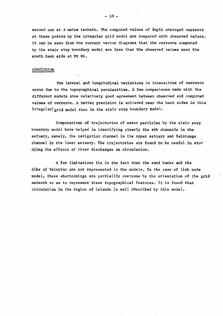
- 59-

second one at 4 metre isobath. The computed values of depth averaged currents

at these points by the irregular grid model are compared with observed values.

It can be seen from the current vector diagrams that the currents computed

by the stair step boundary model are less than the observed values near the

south bank side at PK 86.

CONCLUSION

The lateral and longitudinal variations in intensities of currents

occur due to the topographical pecularities. A few cornparisons made with the

different rnodels show relatively good agreement be~ween observed and cornputed

values of currents. A better precision is achieved near the bank sides in this

irregular'l grid model than in the stair step boundary model.

Computations of trajectories of water particles by the stair step

boundary model have helped in identifying clearly the ebb channels in the

estuary, namely, the navigation channel in the upper estuary and Saintonge

channel in the lower estuary. The trajectories are found to be useful in stu­

dying the effects of river discharges on circulation.

A few limitations lie in the fact that the sand banks and the

dike of Valeyrac are not represented in the models. In the case of link node

model, these shortcomings are partiallly overcome by the orientation of the grid

network so as to represent these topographical features. It is found that

circulation in the region of islands is well described by this model.

APPENDIX I

Instantaneous current vector diagrams

(Stair step boundary madel)

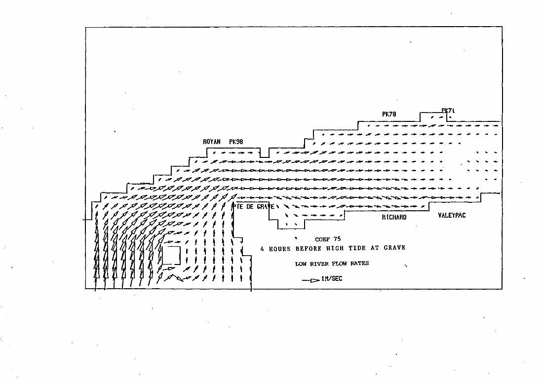
ROYAN PK98

' .. ' .. ..

VALE't'PAC

PK64

4 HOURS BEFORE HIGH TIDE AT GRAVE

COEF 75

LOW RIVER FLOW RATES

lN/SE~

" ILE PHILIPS

ST.CHRISTOLY 8 ILE PATIRAS

·- c ILE NOUVELLE

BEC 0 AMBES

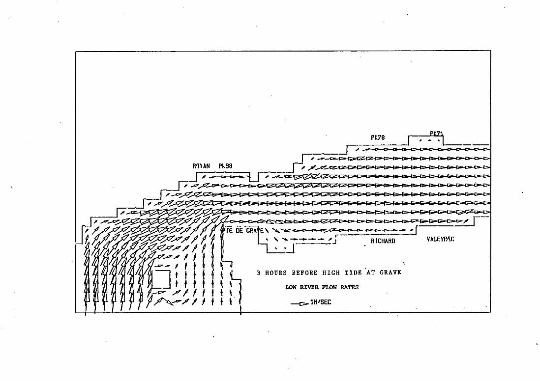
P~7B _j~----

. 3 HOURS BEFORE HIGH TIDE AT GRAVE

LOW RIVER FLOW RATES

--c>1tt'SEC

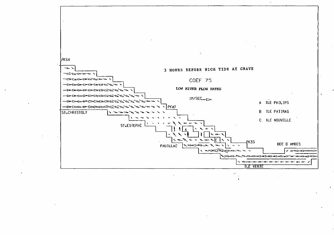
PK64

~---c::..-c:...'-(::,. ~-- '

~---c::..--c::..-c:... ~ 'c::.. ~-- ' ~--c::..~ ""-c::,.. 'c::.. ~ 'c::.. 'c::,:._-c> ____ .... -

3 HOURS BEFORE HIGH TIDE AT GRAVE

COEF 75 LOW RIVER FLOW RATES

lM/SE~

~~~~~'t::....~~----... ...... ...

ST.CHRISTOLY

A ILE PHIUPS

B ILE PAT IRAS

C ILE NOUVELLE

BEC 0 AMBES

P.OYAN Pt-.99

LOW RIVER FLOW RATES

--t:> tH/SEC

VALEYMC

PK64

2 HOURS BEFORE HIGH TIDE AT GRAVE

COEF 75

LOW RIVER FLOW RATES

lM/SE~ A ILE PHILIPS

B ILE PAT IRAS

C ILE NOUVELLE

•

PK78 _EK7 J

1 . - 1 J / _.,.

-"' " --- - w ~ ~ -

ROYAN PK98 /,;rf~- ... ... ... -~ -.. ,.

COEF 75

LOW RIVER FLOW RATES

-C> lM/SEC

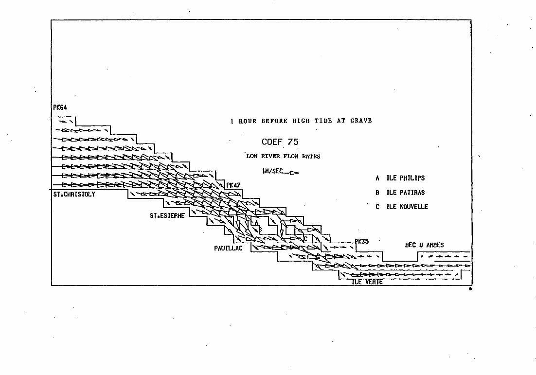
P~64

HOUR BEFORE HIGH TIDE AT GRAVE

COEF 75 .LOW RIVER FLOW RATES

lH/SEC-.t> A ILE PHILIPS

B ILE PAT lAAS

C ILE NOUVELLE

, ..................

•

l

. PK71 PK78 l 1 1 , ---- __.,..

.. _ _.,..~~~ -ROYAN PK98 / _/_..(7'-'Z -~

, .- -V""---t:7_A;?"_..ç?'"__.ç;>"~ ~ ~ ..... ,.._ J' .-po ---c:::---c>-e:... ... .. .. .. -- ...

... ..-/,. ~ ~ - - - ~ ~ ,.._ .,., ,..., - -.. .... ,...-/~

~ ~ .. ... -. ~ ...... -,. - ..... -,_ , "' / _.t7 _......ç7 A ..-? ~ .. - -... "' -... -.. ... " .. ...

1, -....t7--v""_v"'//~~/~.-?" -~ -·~ .,... - ~

~ • - -./...<?..-<T.-<7.-<7/// _, YfX~~~- ~ ... r-/ ////~~~_//',#/ / ~ ~I>TE DE GRA E\. ~----~_.po~-'' 1 / //////// / / / ~ ' -- - -- -- - " r RICHARD VALEYRAC

\ t 1. 1 /.~ //// 1 1 1 , t J ~ etl.l/_,,,,, tt HIGH TIDE AT GRAVE ~ . a t 1 , ' ' ' \ \ ' ' ) ( 'D , , , ' , \ COEF 75

1 1 ' t t ' \ \

1. .-'(? , 1. f , t t ' LOW RIVER FLOW RATES

cf. ,1 j ~ ~ 1 - 1 1 , 1 1 1 ---c:> 1 N/SEC \

PK64

STaCHRISTOLY

HIGH TIDE AT GRAVE

COEF 75 LOW RIVE~ FLOW RATES

1H/SE~ A ILE PHILIPS

B ILE PATIRAS

C ILE NOUVELLE

.---"

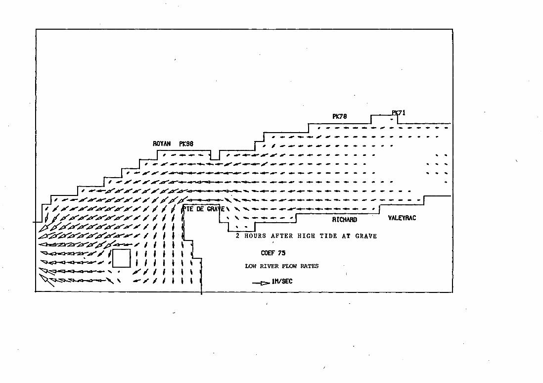
..... ., .. - - .. ROYAN ~98

,.,..,,,....,ca.,.,...,... ........... ...,....,. ... ...,.. .... <~' ............ ~ .. --­

VALEYRAC

HIGH TIDE AT GRAVE

' ' '

COEF 7~

LOW RIVER FLOW RATES

-c>ltt/SEC

.. .. .. ... .... .. .. ..

PK64

ST.CHRISTOLY

2 HOURS AFTER HIGH TIDE AT GRAVE

COEF 75 LOW RIVER FLOW RATES

A ILE PHILIPS

B ILE PATIRAS

C ILE NOUVELLE

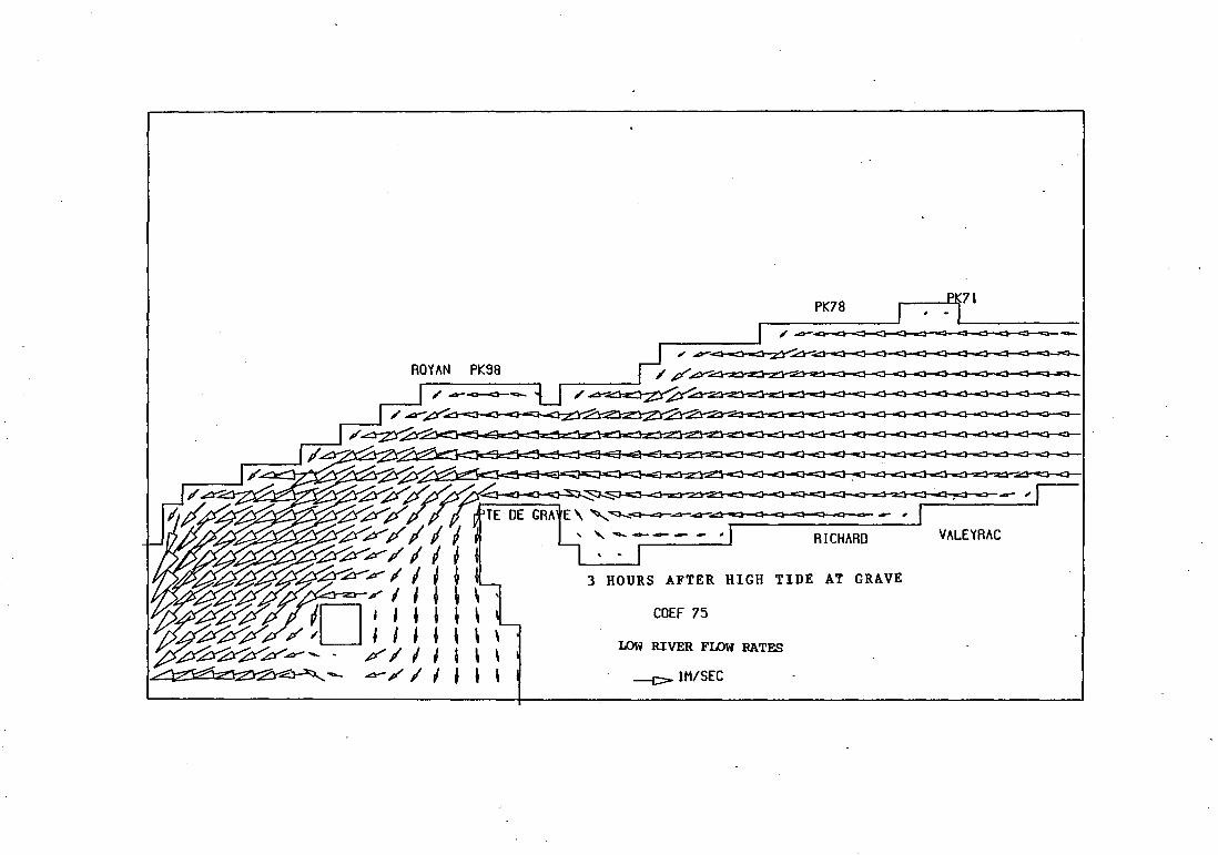
ROYAN PK98

\

' '

COEF 75

LOW RIVER FLOW RATES

· --t> lM/SEC

PK78

VALEYRAC

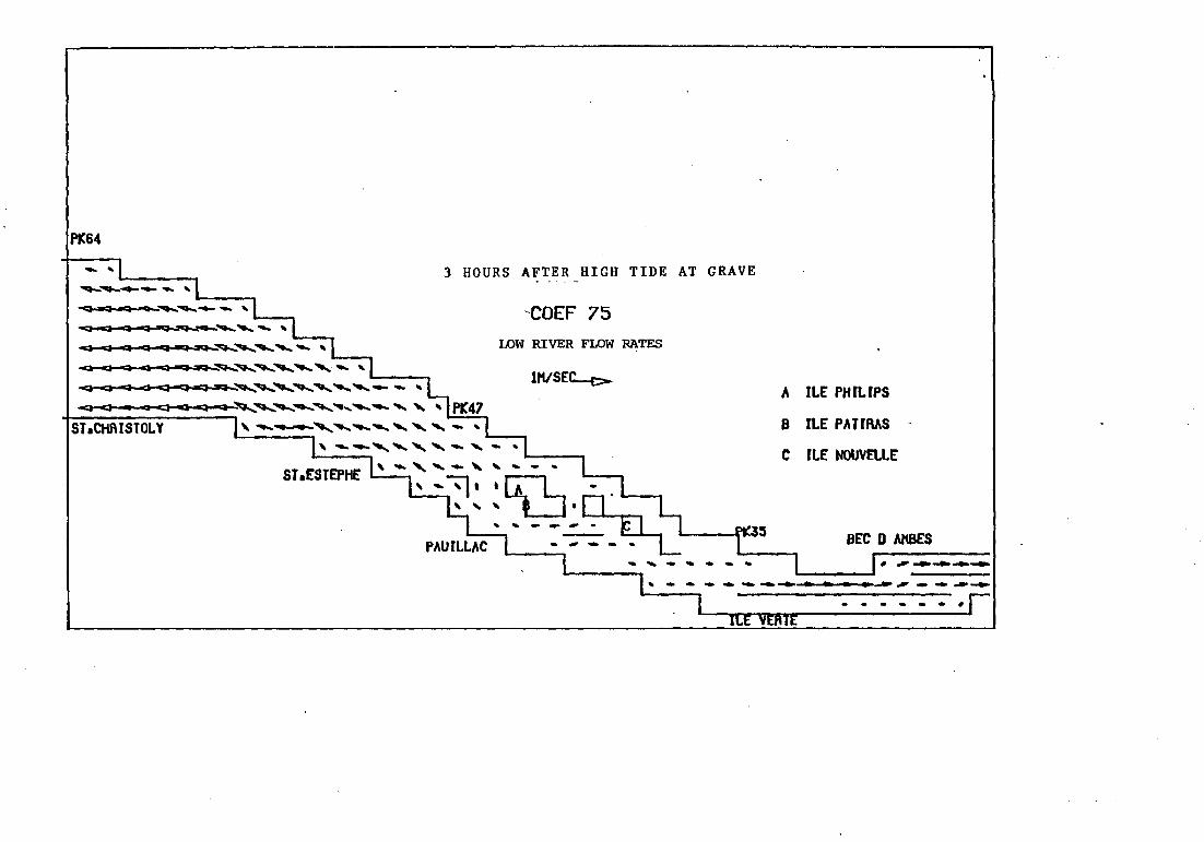
PK64

- ...

QQ~4Q~~~~~~~,~~--'

qq•~QQqq~~~~~~~-,,

ST.CHf\ISTOLY

3 HOURS AFTER HIGH TIDE AT GRAVE

-COEF 75

LOW RIVER FLOW RATES

111/SEC-...e> A ILE PHILIPS

B ILE PAHRAS

C ILE NOUVElLE

- . - - . .. .

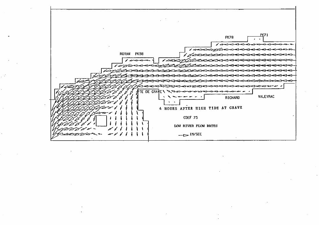
ROYAN PK98

\ \

'

COEF 75

LOW RIVER FLOW RATES

-C> lN/SEC

PK78

VALEYRAC

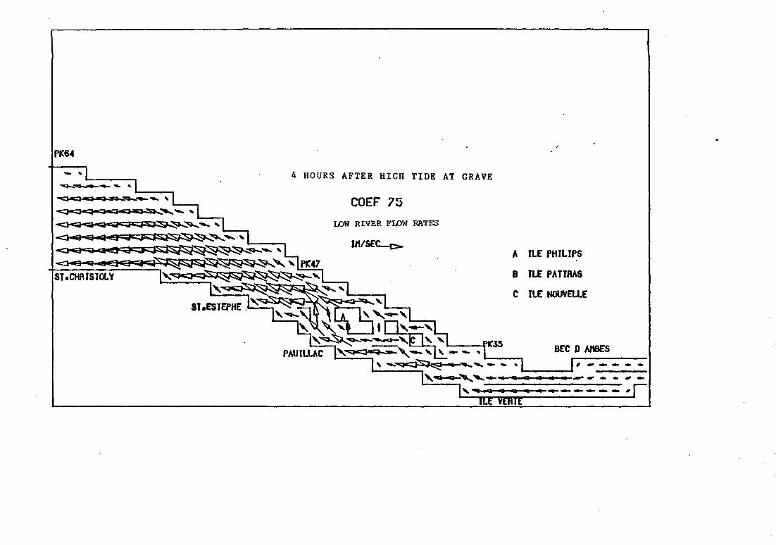
PK64

-' 4 HOURS AFTER HIGH TIDE AT GRAVE

COEF' 75

LOW RIVER FLOW RATES

U1/SEC-.e:-A ILE PHILIPS

8 ILE PATIRAS

C ILE NOUVELLE

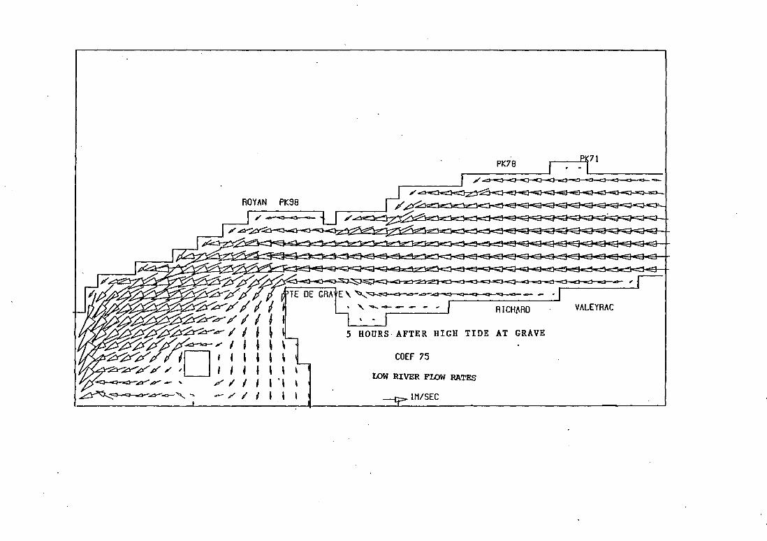
ROYAN PK98

COEF 75

LOW RIVER FLOW RATES

lN/SEC

PK78

VALEYRAC

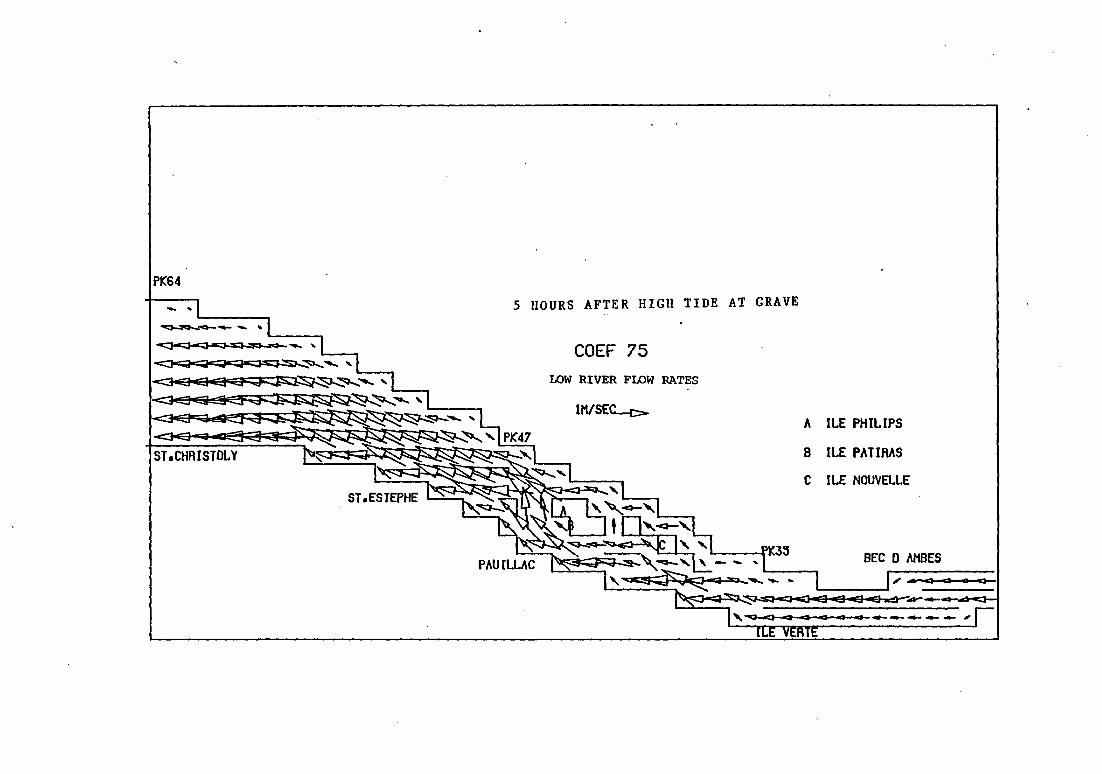
PK64

5 HOURS AFTER HIGH TIDE AT GRAVE

COEF 75 LOW RIVER FLOW RATES

lM/SELc:> A ILE PHILIPS

B ILE PATIRAS

C ILE NOUVELLE

PK78

ROYAN PK98

VALEYRAC

GRAVE

' ' ' ' COEF 75

1 ' ' ' \ LOW RIVER FLOW RATES 1 1 ' \ '

, 1 1 \ ' ---c> lM/SEC

PK64

- ... LOW TIDE AT GRAVE

COEF 75 LOW RIVER FLOW RATES

lM/SE~ A ILE PHILIPS

B ILE PATIRAS

C ILE NOUVELLE

,_. :a ~ 1 a ____ __.

APPENDIX II

Instantaneous current vector diagrams

(Irregular grid finite difference model)

5 HOURS BEFORE LOW TIDE AT GRAVE

COEF 75 Pt-78

LOV P.lvER FLOW P.ATES

P.O YAN Pt. SB

....

.. , "' --- - ~ .......... __. .... ~_.._.,.._.~.,., ...................... _..._.,_.._.._..._,........,.....,.t:rl>' ~ , , , _,

"" - --- - ............. ...,.__.._..,..,., ................. ~ ...... ---~~_... .......... ~ .......... ---, , , 1 ~ ~ _, .... --- ---- -- - _.,. ............ _. ... , 1 1 1 1 1 1 .... ... ""

' ' ,

t 1 ' P.lChAP.D VALE,P.AC

\ \ \ \ \ .. \ ' \ ' \

1 ..

0 \ ' \ ' \

1 1 .... - ' \ ' 1 1 , #' ... ' ' ' ' ! M/SEC -{>

' / - .... - - .. '

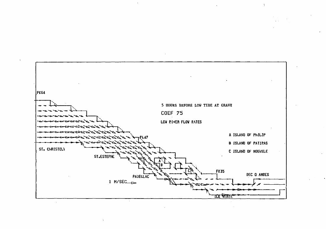
PIC64

ST. ChRISTOL'

1

5 HOURS BEFORE LOW TIDE AT GRAVE

COEF 75

LOV P.l~ER FLOW R\TES

A ISLAND OF PhiLIP

B ISLAND OF PAT1P.AS

C ISLAND OF NOUIELE

BEC D AHBES

iii • J' , ----1

1

4 HOURS BEFORE LOW TIDE AT GRAVE

COEF 75 Pl-.78

LOV RIVER FLOW P.\fES

P.O\ AN Pk.98

1 M'SEC --t>

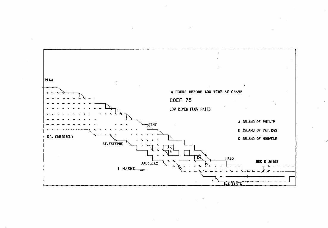
PK64 . r--,_ 4 HOURS BEFORE LOW TIDE AT GRAVE -- T'-,_ .................. .--

... l COEF 75 - - - - - ... ... .... r ', LOV P.IVER FLOW ft\TES - - - - - - - ... .. ... ... 1"',, - - - - - - . ' . . . ' r---- - - - - - .. ... . . A ISLAND OF PHILIP ', --- - - - - - .. ' . . . ~K47

' ' B !S~AND OF PATlA~S .. . ' • . - .. . . L_ .. ,

' ~ ~ . ... ... .. . Sf a CHRISTOLY ' r ',, C ISLAND OF NOU~ELE ' ... ___ . .. ' "' . ST.ESTEPHE ..

:-1 \

~ ' ~ ' ' ~ PK35 ..... ' ' -- '• '·-a BEC D AH9ES PAU:LLAC ~:,, , •. 1 ' ~- - -' - - l J,.,. 1 MISE~ , , ....... --.. ........ .... '- • • 11',

' \ ... IL[\'~;,~ : 1 \ •

3 HOURS BEFORE LOW TIDE AT GRAVE

COEF 75

. L0\1 RIVER FL0\1 RUES

R!CHARO VALEYRAC

1 H/SEC -t>

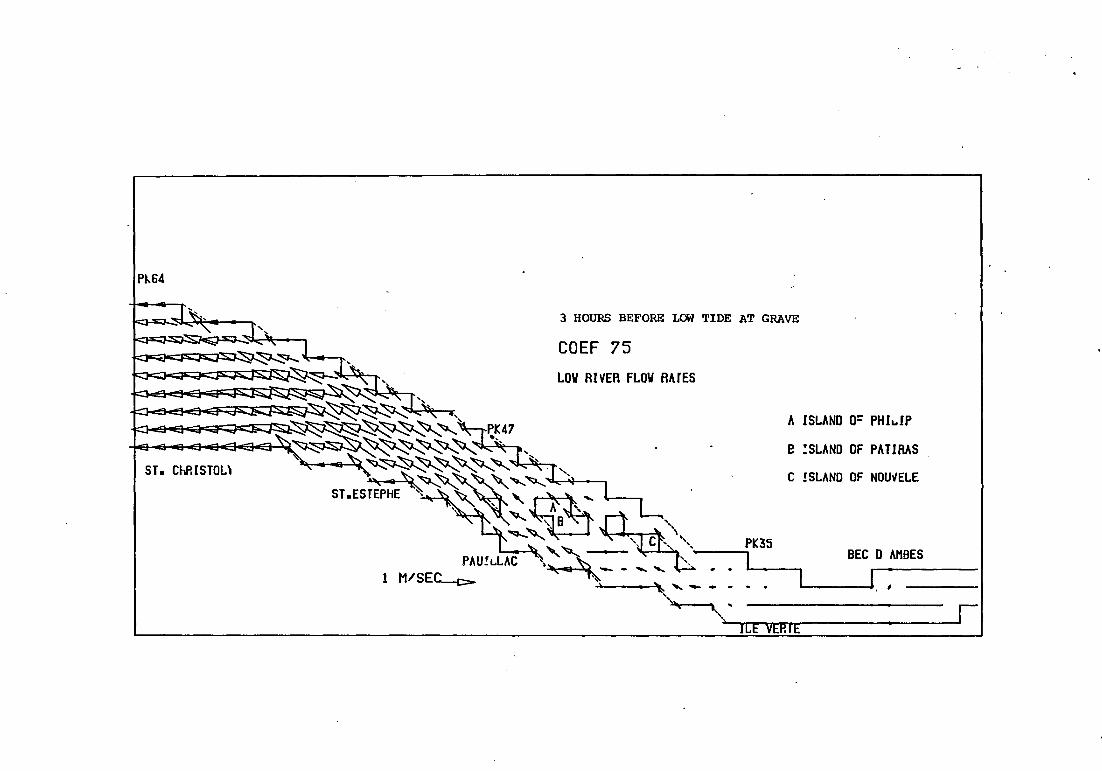
P._64

ST. ChRISTOL\

3 HOURS BEFORE LOW TIDE AT GRAVE

COEF 75

LOV RIVER FLOV RArES

. __ ...;Pt::35

1 PAU!LL_A __ C _.__.," 1 M/SE~ 'oa -1\-.- - - '

) ~ ' ........

A ISLAND o= PHI~IP

e :SLANO OF PATIRAS

C !SLAND OF NOU~ELE

BEC 0 AHBES

'----_,1. 1

''\...._ ' ·<· 1 ~rmcE~vE~r.~rE--------------~

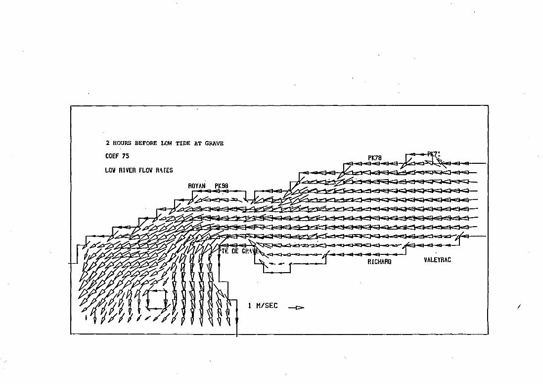
2 HOURS BEFORE LOW TIDE AT GRAVE

COEF 75

LOV RIVER FLOV R\fES

1 H/SEC

RICHARD VALEYRAC

/

PK64

SI". CHRISI"OLY

PAU!a...LAC 1 M/SEC-.c::-

2 HOURS BEFORE LOW TIDE AT GRA\~

COEF 75

LOV RIVER FLOW P.~TES

A ISLAND OF PHILIP

B ISLAND OF PAfiA\S

C ISLAND OF NOUVELE

BEC D AMBES

..,__ __ _Jl -

lit- ....... --·-------

.... ------------------~~---------------------------------'~:g~mr r-~~~~F~'~E~A~rE~------------~

1 HOUR BEFORE LOW TIDE AT GRAVE

COEF 75

LOV RIVER FLOV RATES

VALE\RAC

1 M'SEC -(>

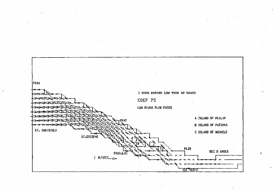
PK64

ST. CHRISTOLY

PAUILLAC ' MISE~

1 HOUR BEFORE LeM TIDE AT GRAVE

COEF 75 LOW RliEP. FLOW P.ATES

A !SLAND 0~ PhiLlP

B ISLAND OF PATIR~S

C ISLAND OF NOUVELE

BEC 0 AM3ES

• • L ;a.s ....

.... ~

-~~~~~L~F~~v~EAnl_~;--------------_j,-·----------------~

1

LeM TIDE AT GRAVE

COEF 75 PK78

LOV RIVER FLOV P.\rES

RDlAN PK98

PK64

sr. ChRISTOL\

PAUil.LAC 1 MISE~

LOW TIDE AT GRAVE

COEF 75

LOV P.lVER FLOW R\rES

A ISLAND OF P~lwlP

e IS~ANO OF PAriP.~S

C IS~AND OF NOUVELE

BEC D AHBES

lii.J ____ _

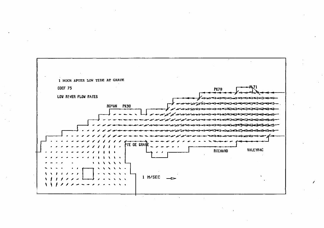
1 HOUR AFTER LOW TIDE AT GRAVE

COEF 75

LOW A!~EA FLOW P.~rES

ROYAN Pk.98

,____PK-78 __ ;;: : ~, .. .. .. ~~~~~~~~~~~~~~~~~~~~~~­

r-----~~~~~~~~~~-<~~~~~~~~~~Er~--

-~--~--~~~~,,~/~~~Qd

.,. - ----------~- oc:~ ... ----~A"'ôd--c::~-J-Q-oc::)o<....,..o-;QoooElc::!I"E:to=:;;;Jo;;;;;;;;aloEaoe:S.I!S~r-

,., #' #' "' ; ; , ~-- ---- - ______ _...~.,.Y"---------~~ Jf-4-----

_,#'//ll~/ '~---

, , .. .. , ,

- .. ' ' .... 1 ,,,,,,, ' 1 1 1 "' "' ...

,. / "' 1 1 1

.. , \

\ ' 0 ' \

- ... .... , .. ...

\

' '

' ' \ ' 1 / / "' - - - ~ , .. • .. '

RICHARD YALE'tR~C

.. 1 M/SEC ---(:::>

1

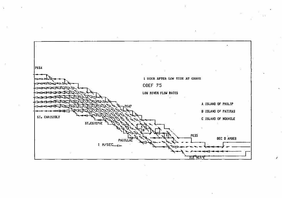
PK64

ST. CliRISTOLY

PAUILLAC 1 MISE~

1 HOUR AFTER LOO TIDE AT GRAVE

COEF 75

LOW RIVER FLOW RATES

A ISLAND OF PHILIP

B ISLAND OF PATIP.AS

C ISL~ND OF NOUVELE

BEC D .AMBES

~ ....... -. ...-...} -- ----..... 1

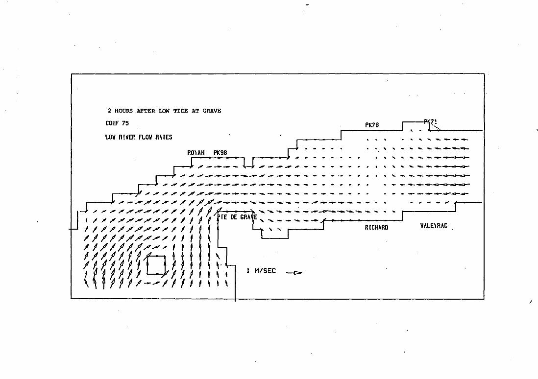
2 HOURS AFTER LOW TIDE AT GRAVE

COEF 75 _01'"7t .-----P_K7_s _ ___,l , , J-e,..·-.::,;:.,.._ __ _

1 LOV R!~EP. FLOV R\rES . . . P.Q)AN PK98 r---_, , , - - . .. - . ' ' ' .... ... .......... ~---~

,__.-~l tt!" ... ~........ .,.,.,..,. .... .,., ... - ..... # ~ • ' ' .... " ..... ~~ .. Cl ::e:)-=-

.---_,~.., "-------------" ....... ---- - - ·- .. 1 ,. • ' .... - ..... -----Cl Cl <3" C" J.., _ _,....,. __________ _, .... __ ------ ... ,. . -- ____ ..,.Cl Cl~

....----P , ,., , ;l' / "",., _,......,. ........... ---~ ............. ~ ..... ..... .... ~ -- ... .... - • • • .. .. -- -- ..... ~..-ca--.4-

.------JI-,L "...-:..""'""'....,. _, "/ / /.....,. ______ ............ - .............. - - _, ------- - , , • , ,., - .., 1~~------

u " .., -" / , ~...,""'""' / / 1 1 1/" ..................... - ~ -- ---v---------- .. ... 1

1 / / / //./// / / l / l / PrE DE GRA\ E , , __ - .... -- .~--~--------"' 1 1 / /////// / 1 / 1 f , , ) 1 P.lCHARD VALE,RAC

/11/////.//llll\ / 1/11/././~-' 1 f, \ '-111111./.htft f\ 1 H ~ H t w ~ u ll ~- ;- 1 H/SEC --<> ,,~~~l/-./1111 1' '\

1

PK64

S T • ChRISTOl.)

PAUILLAC 1 M'SEL.c:-

2 HOURS AFTER ~ TIDE AT GRAVE

COEF 75

LOV RlVEP. FLOV RATES

A ISLAND OF PhiLIP

B ISLAND OF PATIRAS

C ISLAND OF NOUVELE

eEC 0 AMBES

• ?..- ____ , /

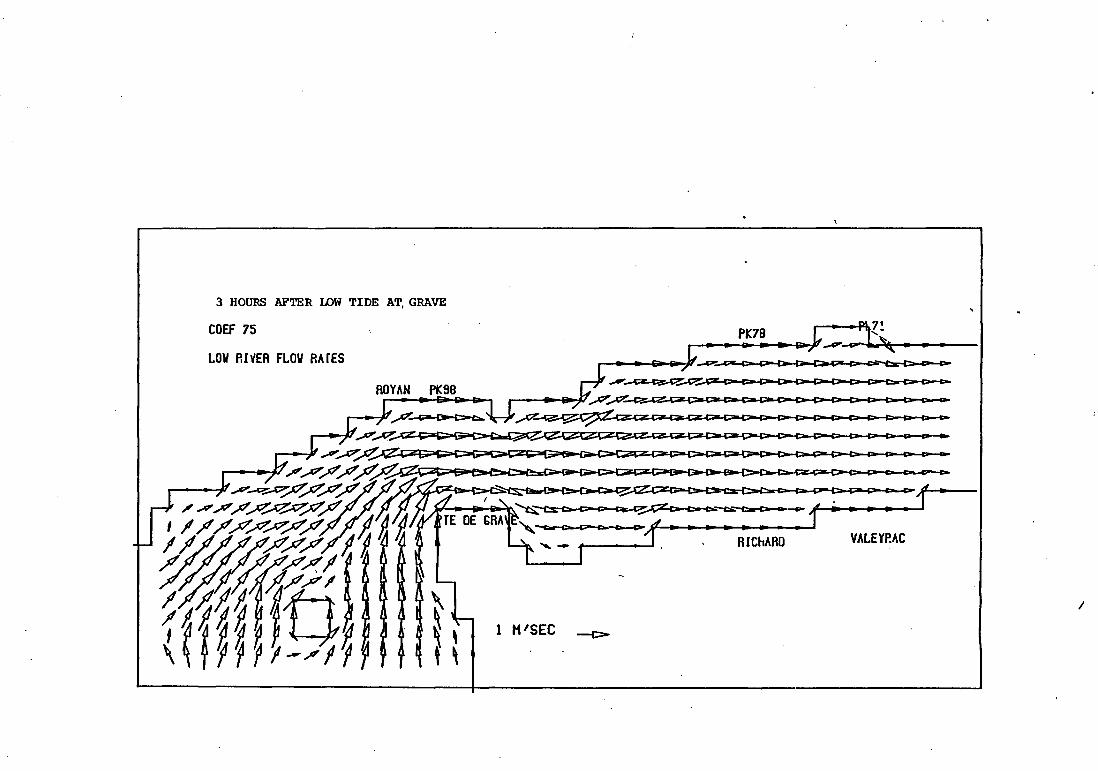
3 HOURS AF TER LOW T COEF 75 IDE A~ GRAVE

PK7B

LOV P.I~ER FLOV P.ArES

VALEYP.AC

1

l M'SEC

PK64

sr. CHRlSI"OL\

. -

PAU!L.LAC 1 M1SELc:,..

3 HOURS AFTER LOW TIDE AT GRAVE

COEF 75

LOV RIVER FLOW RATES

A ISLAND OF PhiLIP

e ISLAND OF PArlP.AS

C ISLAND OF NOU/ELE

BEC D "AMBES

~ ~rE~a~, ~ -------1 .. Iii ::e •

1

4 HOURS AFTER L0W TIDE AT GRAVE

COEF 75

LOV RIVER FLOV P.ATES

RlCHARO VALEYR~C

1 M/SEC --C>

PK64

sr. CHRISI"OLY

4 HOURS AFTER LOW TIDE AT GRAVE

COEF 75

LOV A!VER FLOV A~fES

A ISLAND OF PHIL!P

B ISLAND OF PATIRAS

C ISLAND OF NOUVELE

BEC D AMBES ~ j __ ____ , : li ~

1

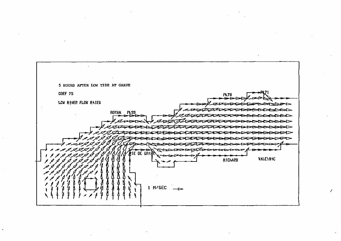
5 HOURS AFTER LOW TIDE AT GRAVE

COEF 75

LOV R1VEP. FLOV R~rES

1 MISEC

Pt.7B

1

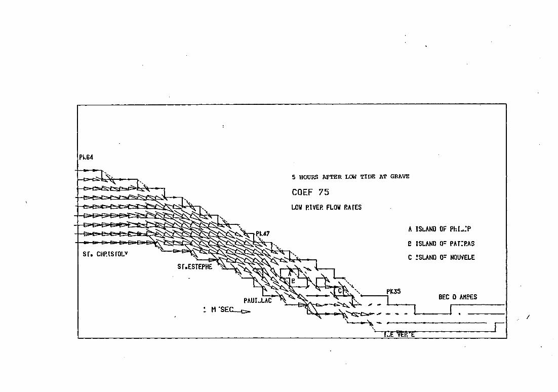
P~64

sr. CHP.tSrOLV

5 HOURS AFTER LOW TIDE AT GRAVE

COEF 75

LOV P.lVEP. FLOV P.ArES

A IS~ANO OF Phi~:P

e ISLAND o~ PAT:P.AS

C !SLAND o= NOU~ELE

__ ....;,PK35 j BEC 0 AH~ES

"' - .&.-. ---.,___--JJ . ~--~~- -----------~"fift;E~r.·~E _____ __Jr

6 HOURS AFTER LOW TIDE AT GRAVE

COEF 75 Pk78

l.OV ftl/EP. Fl.OV P.ArES

P.OYAN PK98

VAl.Elft\C

:M'SEC

Pt::64

sr. CliP.ISrDl.'f

6 HOURS AFTER LOW TIDE AT GRAVE

COEF 75

LOW RI~EP. FLOW R\TES

A ISl.ANO OF P~l~IP

p :St.ANO OF PATIRAS

c ISLAND o= NOUVELE

BEC 0 AM~ES

APPENDIX III

Instantaneous current vector diagrams

(Link node madel)

40'

35'

45 30'

20'

151

101

os'

5 HOURS BEFORE HIGH TIDE AT GRAVE -· -COEF 70

LOW RIVER FLOW RATES

--1 mts

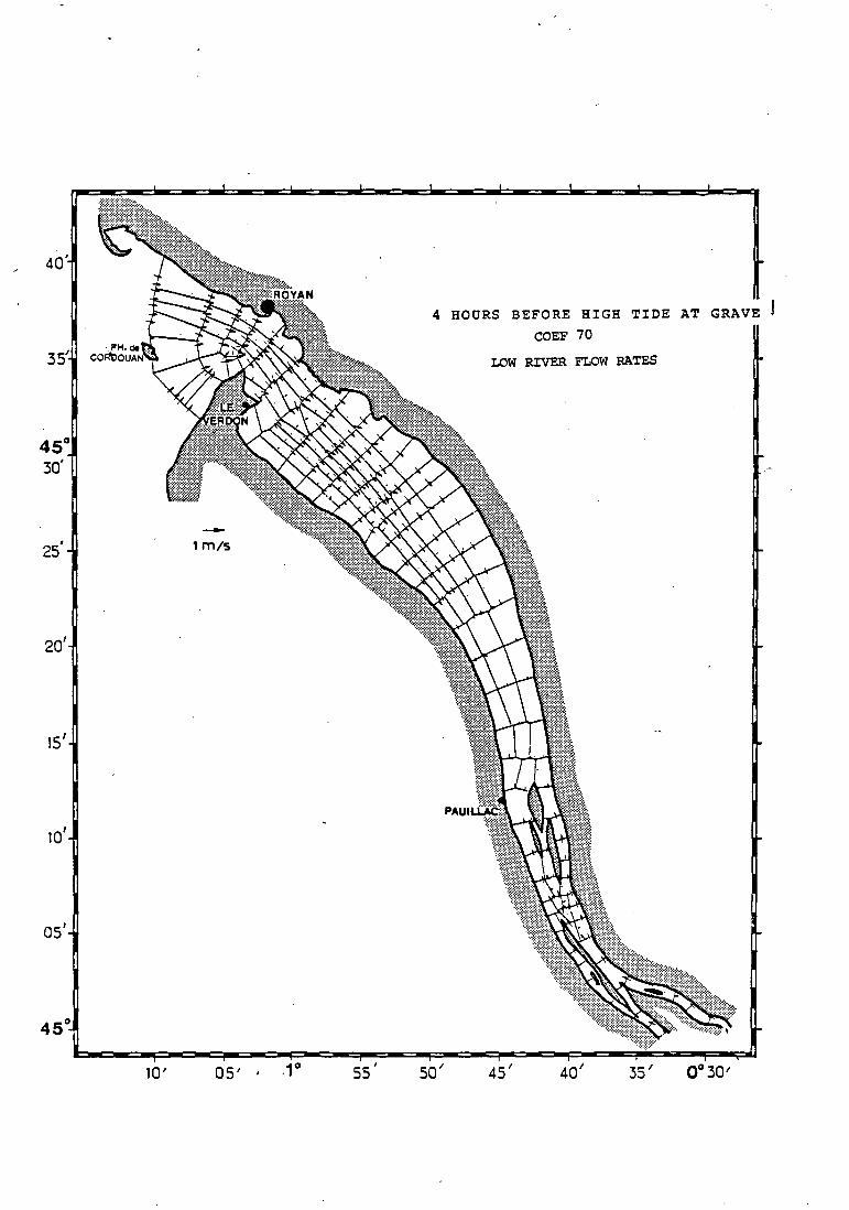
40'

3

-1m/s

20'

1S'

10'

os'

10' ss'

4 HOURS BEFORE HIGH TIDE AT GRAVE j COEF 70

LOW RIVER FLOW RATES

sa' 45 1 40

1 3S 1

40'

35'

45 30'

20'

15'

10'

10'

-1mts

OS' 55'

3 HOURS BEFORE HIGH TIDE AT GRAVE

COEF 70

sa' 4S' 40' 35'

40'

•

35'

-1m/s

20'

15'

10'

os'

10 1 05' 55'

2 HOURS BEFORE HIGH TIDE AT GRAVE

. COEF 70

LOW RIVER FLOW RATES

5o' 45 1 40 1 35'

40'

35'

-1m/s

20'

151

10'

os'

10 1 05' 55'

1 HOUR BEFORE HIGH TIDE AT GRA

COEF 70

LOW RIVER FLOW RATES

501 45' 40' 35'

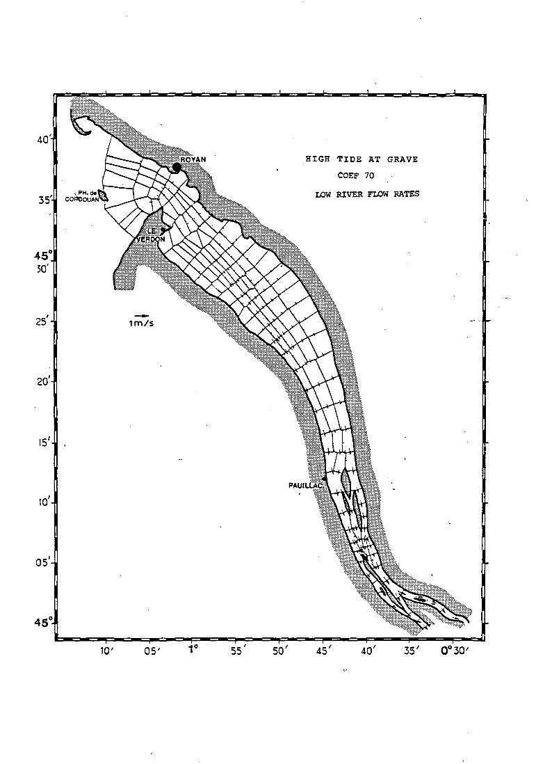
40'

35'

-1m/s

20'

151

101

os'

10 1 05' ss' sa'

HIGH TIDE AT GRAVE

COEF 70

LOW RIVER FLOW RATES

45 1 40

1 35 1

3

-1m;s

20'

15'

10'

os'

lQ' 05' ss'

1 HOUR AFTER HIGH TIDE AT GRAVE

COEF 70

LOW RIVER FLOW RATES

sa' 45 1 40 1 35 1

40'

35'

--1m/s

20'

151

10'

os'

10 1 05' ss'

2 HOURS AFTER HIGH TIDE AT GRAVE COEF 70

LOW RIVER FLOW RATES.

45 1 40

1 35 1

40'

3 3 HOURS AFTER HIGH TIOE AT GRAVE--COEF 70

LOW RIVER FLOW RATES

-1m1s i

20'

151

101

os'

10' 05' ss' 401 35 1

40'

3 4 HOURS AFTER HIGD TIDE AT CR~VE

COEF 70

LOW RIVER FLOW RATES

-1m1s

20'

151

10'

os'

10' 05' ss' sa' 45' 40' 35' . 0030'

--

40'

5 HOURS AFTE? HIGa ~IDE AT G2AV~

COEF 70

LOW RIVER FLOW FATES

-1m1s

20'

15'

101

os'

10' os 1 ss' sa' 4S'

40'

6 SOURS AFTER HIGH TIDZ AT GRAVE

COEF 70

LOW RIVER FLOW RATES

-1 m/s

20'

15'

10'

os'

10 1 OS' ss' sa' 45 1 40' 35 1

CHAPTER IV

RESIDUAL CIRCULATION IN THE GIRONDE

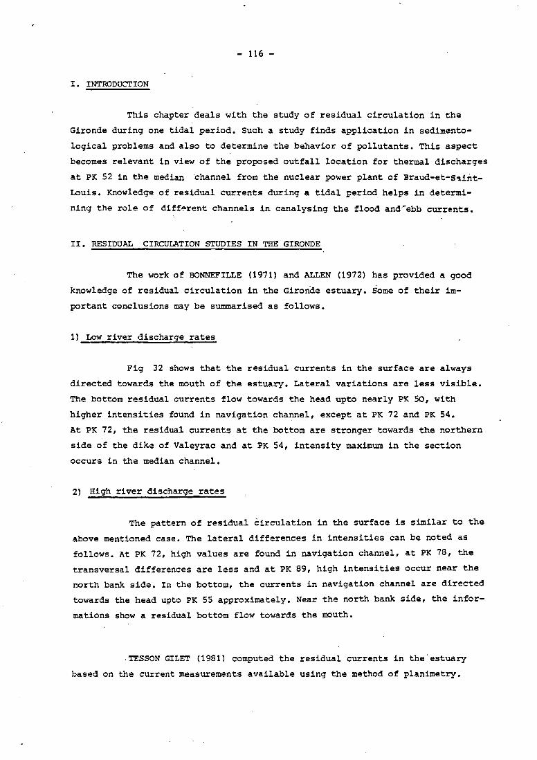
- 116 -

I • INTRODUCTION

This chapter deals with the study of residual circulation in the

Gironde during one tidal period. Such a study finds application in sedimento­

logical problems and also to determine the behavior of pollutants. This aspect

becomes relevant in view of the proposed outfall location for thermal discharges

at PK 52 in the median channel from the nuclear power plant of Braud-et-Saint­

Louis. Knowledge of residual currents during a tidal period helps in determi­

ning the role of diffl?!rent channels in canalysing the flood and·-ebb currE>nts.

II. RESIDUAL CIRCULATION STUDIES IN THE GIRONDE

The work of BONNEFILLE (1971) and ALLEN (1972) has provided a good

knowledge of residual circulation in the Gironde estuary. Some of their im­

portant conclusions may be summarised as follows.

1) Low river discharge rates

Fig 32 shows that the residual currents in the surface are always

directed towards the mouth of the estuary. Lateral variations are less visible.

The bottom residual currents flow towards the head upto nearly PK 50, with

higher intensities found in navigation channel, except at PK 72 and PK 54.

At PK 72, the residual currents at the bottom are stronger towards the northern

side of the dike of Valeyrac and at PK 54, intensity maximum in the section

occurs in the median channel.

2) High river discharge rates

The pattern of residual èirculation in the surface is similar to the

above mentioned case. The lateral differences in intensities can be noted as

follows. At PK 72, high values are found in navigation channel, at PK 78, the

transversal differences are less and at PK 89, high intensities occur near the

north bank side. In the bottom, the currents in navigation channel are directed

towards the head upto PK 55 approximately. Near the north bank side, the infor­

mations show a residual bottom flow towards the mouth •

. TESSON GILET (1981) computed the residual currents in the'estuary

based on the current measurements available using the method of planimetry.

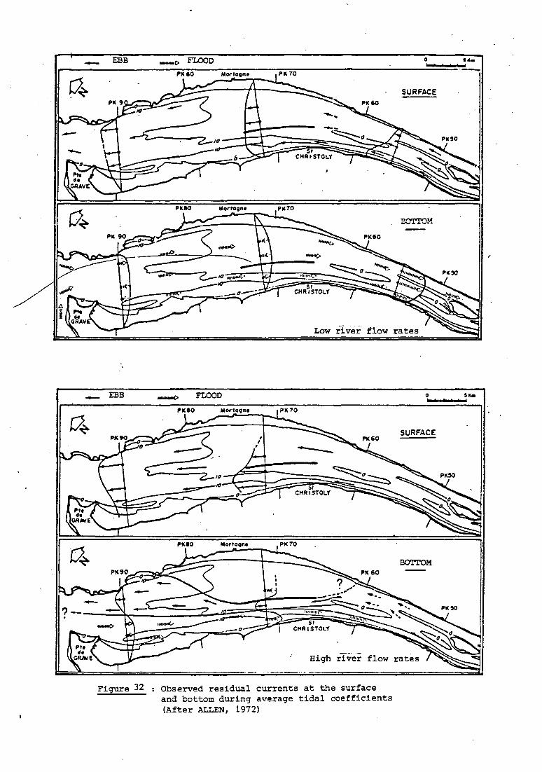
r o~

- EBB

Figure 32

SURFACE

EOTTOM

Law river flow rates

FLOOD

SI CHRISTOLY

0

SURFACE

BOTTOM

High river flow rates

Observed residual currents at the surface and bottom during average tidal coefficients (After ALLEN, 1972)

PK !10

PK 89 PK 78 PK71 PK67·

' ' \~ Y<. ' ' \

* \ 0 •

Ao0t l98ll

' ~

' \ * 23 Octobrw 1981

2~ Fivrltr 1971

24 Juin 1971 tt ~(Maral979)

Figure 33 Residual currents at different depths in the navigation channel (After TESSON GILET,1981)

PK 4 2

lsoh1linl ·-.

? 0

Converyenu,divtrgence 111 fond:0,l}

- 119 -

The results, show in figure 33,· show that the intensities are of the order

of 10-50 cm/sec. in the navigation channel, the magnitudes varying with seasons.

The position of the nodal point gets displaced depending on river discharge

rates. Along the navigation channel of the estuary, the maximum intensities

are found at PK 71 and PK 89.

!II. DEPTH AVERAGED RESIDUAL PARAMETERS

A few numerical experiments have been conducted with the different

models used. These involves the computation of Eulerian residual currents,

.Eulerian residual transport velocities and the lagrangian residual displacements

of a water particle at different points in the domain. The former two parame­

ters are calculated as follows.

u = t

1 T -ru dt T o

T r u Cl';.+ h> 0

T (z; + h) r 0

dt

dt

T / 0 V dt

T r v(z; + h) dt 0

vt - T r ( z; + h) dt 0

where, ur and vr are the x and y components of depth averaged resi­

dual current vector and ut and vt are the corresponding components of the depth

averaged transport velocity vector.

The laqrangian residual displacements are evaluated from the computed

trajectories of water particles, as discussed in the previous Chapter.

It is true that the depth averaged Eulerian residual parameters are

only mathematical entities and their physical significance is not much clear.

SALOMON (1976) reported that the study of Eulerian residual parameters coupled

with the lagrangian residual parameters are êomplimentary in the study of

estuarine dynamics.

1) Stair step boundary madel

The principal features observed in the computed field of residual

currents can be summarised as follows (refer, fig 34 to 37). Mean river flow 3 .

rates correspond to a discharge rate of 700 m sec-1.

RESIDUAL CURRENTSI

Figure 34

/ <l-<l--"Q-<1-p-- ................. '-, ...... ....... -- - -- - ........ ..... ' ' . PK99 ___j /Ç~~--- ............. ~ ........... ---------- ..................... -...--

,~,~--- ............... -~,,,~~~--~--~~~~ //~~1/-,,, ___ ,~~~~~~

~ / - / 1 , , 1 1

• 1 / ~ " ' ' -- ·- ....... ~ ~ """"' ...- ..q-..' ~..:a- ..,_

, ___ "" VALEYRAC ;1 - - - -

\

--,1 .... _____ , 1

- - • , 1 ' ___ ,\, - ~ , ,

Al CHARD

COEF 70 MEAN RIVER FLOW RATES

-c> 15 cm/sec

Depth averaged residual currents (stair step boundarl' mdel) during mean river flow rates

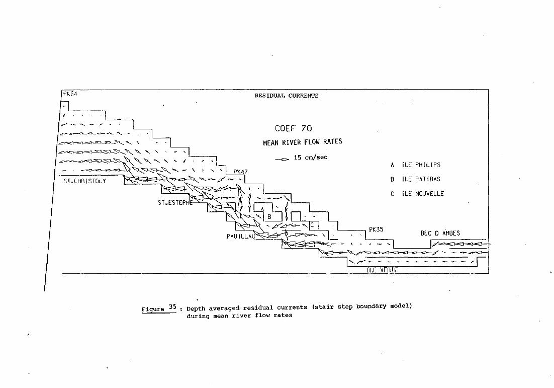
PKG4

l __ ___, ·1------. 1 .

ST.LHR!STOLY

RESIDUAL CU~~NTS

COEF 70

MEAN RIVER FLOW RATES

-c> 15 cm/sec /1. ILE PHILIPS

8 !LE P/I.TlRAS

C ILE NOUVELLE

BEC D AMBES

-' l/~~-~-&~~ 1'->.t<::::J-<!-,~/ ·- - --~

......... ~- - - - - - - ---- , 1 fLE VERTË

Figure 35 Depth averaged residual currents (stair step boundary model) during mean river flow rates

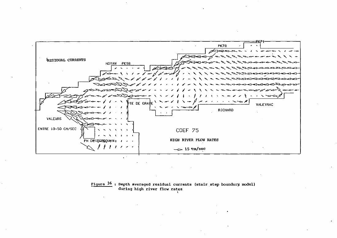
~SIDUAL CURRENTS

ENTRE 10-50 CM/SEC

---<>

" -/ "' , , 1 / - ' ' ....... -- -- --'"Q....<J-«0--<lr-<J--ooEO..:a--o:::l-~P""~

- ,. ; 1 1 ~ ' ' ' ...... - ....... -- --4:)--·--~..a:-P" ...a-40-' <>--4----

' ' ~ / 1 • . f 1 1 ' ..... - ,. .; \ - • ' -.:...-c:;;,..,.~ 1 '-- / 1 ' ~ 1-- .; , -.....~l'

'~JI VALEYRAC

RICHARD

' ....... ' ' \ COEF 75 ' 1

HIGH RIVER FLOW RATES

-c> 15 tm/ sec

Figure 36 Depth averaged residual currents (stair step boundar~ model) during high river flow rates

\

PK64

ST.CHRISTOLY

RESIDUAL CURRENTS

COEF 75 HIGH RIVER FLOW RATES

lOCM .'\ ILE PHILIPS

B ILE P.rH IRAS

C ILE NOUVELLE

BEC D AMBES

Figure 37 : Depth averaged residual currents (stair step ~undary model) during high river flow rates

- 124 -

ln the upper estuary, intense residual currents occur in the

navigation channel. Between PK 35 to ~K 41, residual currents are practically

absent in Blaye channel. Around the islands of Philippe and Patiras a residual

eddy is present. The eddy is in the clockwise direction. It can be seen in the

instantaneous current vector diagrams that (Appendix I), at Pauillac, ebb

currents are strong in between the islands of Trompeloup and Philippe, where

as flood is more predominant near the north bank side. Renee these differences

found during ebb and flood can produce a residual circulation around the

islands. Downstream, between Pauillac and St. Estèphe, the residual currents

are intense in navigation channel. In the corresponding region, the currents

are very feeble at the right bank side. These values are considerably less than

the observed values (fig 32) at PK 54. It means that the residual flow is

concentrated along the principal channel in this region. Downstream, from

PK 60 upto· St. Christoly, lateral differences in the residud current field

are less marked.

In the lower estuary, between St. Christoly and Richard, the

residual currents flow parallel to the coast, with high values observed in

the navigation channel. Downstream from Richard, a transition occurs from the

navigation channel to the Saintonge channel with residual currents tending

to flow from the former to the latter. Also, residual currents become intense

along the north bank side. Near PK 85, a residual eddy is present. The resi­

dual eddy is situated just downstream.of sudden change of residual circulation

from the navigation channel towards the northern channel. In this region, the

presence of bank of Vivian along the south bank side and the deep Saintonge

channel along the north bank side make sharp gradients of depth in lateral

sections. This depth gradient is mainly responsible for the formation of the

res idual eddy.

From PK 87 onwards, the residual flow is downward and the currents

get evacuated to the sea along the south bank side at the Pointe de Grave.

Outside the mouth of the estuary, the residual currents are strong in the passage

of navigation near the northern side. The residual circulation outside the

mouth of the estuary is sensible to the seaward boundary conditions and this

aspect is not discussed here.

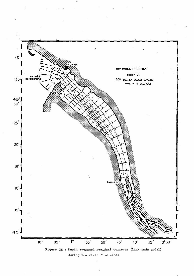
40'

20'

15'

10'

Js'

10' OS'

Figure 38

ss' so'

lŒSIDUAL CURRENTS

COEF 70 LOW RIVER FLOW RATES

--t::==- 5 cm/ sec:

45' 401 35 1

Depth averaged residual currents (link node model)

during low river flow rates

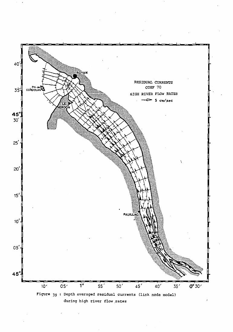
40'

45 30'

20'

15'

10'

os'

10'

Figure 39

05' ss' sa'

RESIDUAL CURRENTS

COEF 70

HIGH RIVER FLOW RATES

--1:> S c:m/.sec

45' 40' 35'

Depth averaged residual currents (link node model)

during high river flow ,rates

0°30'

- 127 -

Fig 36 to 37 represent the residual currents computed for high

river discharge rates (1300 m3/s). The phenomena observed are quite similar

to the case of low river flow rates. In this case, the magnitudes of residual

currents are higher and the residual eddies are more pronounced than in the

previous case. The high intensities are particularly marked in the regions

which canalyse ebb, namely the navigation channel in the upper estuary and

the Saintonge channel between PK 80 - 92. When the discharges are high,

between PK 75 - 80, the residual currents at the 'South bank side are directed

towards the mouth. In the case of low river discharges feeble residual currents

directed towards the head are found at the south bank side of this region.

2) Link node madel

Eulerian residual currents are computed as in the case of stair

step boundary model. Here, the integration over a tidal period is made of

one dimensional current vectors. The computations involve both the cases of

low river discharges (183 m3/s) and high river discharges (1300 m3/s).

The results are presented in figures 38 to 39.

In the upper estuary, residual currents are found to be maximum

in the navigation channel. Between PK 35 to PK 41, the magnitudes of residual

currents in the Blaye channel and in the navigation channel are found to be

the almost same, which is different from the results of the stair step boundary

madel. Between the islands of Philippe and Bouchaud, there is a small residual

current flowing towards the head. In the same region, a clockwise residual

eddy is observed in the case of stair step boundary madel. These two results

are comparable. At PK 52, residual currents are maximum in the navigation

channel and feeble values are~observed in median channel.

Between PK 55 to PK 60, the transversal variations in residual

currents are not much marked. This is true in the case of stair step boundary

model also for this region. Downstream, high intensities in residual currents

are found in navigation channel. From Richard onwards upto nearly PK 85, small

residual currents tend to flow towards the northern channel and at PK 90,

maximum residual current is observed in the northern channel. Between Richard

and Verdon, residual currents are extremely feeble at the south bank side.

- 128 -

This is a region of low depths due to the presence of sand banks. At Verdon,

lateral differences are absent. At Grave, the intensity of residual currents

occurs at the south bank side.

In general, the results obtained above are in agreement with the

stair step boundary model results. An exception is observed in the Blaye

channel in the upper estuary.

3) Lagrangian residual parameter

The residual displacements of a water particle during a tidal period

are computed by the same method as that of trajectories of water particles,

as described in page 50. The calculations are .done using stair step boundary

model.

The results are presented (figures 4Q to 4.1) for low river flow 3 rates{183 m7sec). Moreover, a few results can be seen in the diagrams of

trajectories (figures 25 to 27) in Chapter III. It is to be noted that

the lagrangian residual displacements depend on the instant of departure of

a water particle. In figures 40 to 41, the instant of start is approximately

middle of flood tide at Grave.

Fig. 40 shows that in general, the residual displacements are towards

the mouth in the lower estuary. Between Richard and St.Christoly, the maximum

displacements of water particles occur in the navigation channel. In the same

region, the residual displacements are small along the south bank side and

practically absent along the north bank side. From PK 80 onwards upto Grave,

high displacements are found in the Saintonge channel. These are similar results

to those obtained in the case of Eulerian residual parametres.

In the upper estuary, the pattern is more complicated. For a given

instant of departur'l! as in figure 4·1, the ·following aspects can be concluded •

Bigh residual displacements directed towards the mouth of the estuary are

present in the navigation channel. Along the north bank side, the residual

LAGRANGIAN R~~IDUAL DISPLACEMENTS

PK78 Prl & ... .... • • ... •

ROYAN PK98 "'"-->< ~ """"->< .~ ~ ~ lill>

~~~ .......... ~ ~ .do...,.c ....._ ~·......__ ......_ ......_ ....._

~ .t!f- .1!1: {t î ~ ""'-< ..,._.. ~ ~ ..-_ ----.. ...._ ----..

~ "" "" 4< .do>< .l ~ ~ Aoc ~ ~1

RICHARD VALEYRAC

0 COROOUAN

~ ARRIVING POINT COEF 75

LOW RIVER FLOW RATES X STARTING POINT

Figure 40 Lagrangian residual displacements during law river flow rates

PK64

X STARTING POINT

A ARRIVING POINT

/

ILAGRANGIAN RESIDUAL DISPLACEMENTS

COEF 75 LOW RIVER FLOW RATES

A ILE PHILIPS

B ILE PATIAAS

C ILE NOUVELLE

.. RTE

Figure 41 Lagrangian residual displacements during low river flow rates

- 131 -

displacements are practically absent. In the central region between St. Estéphe

and Ile Verte, the water particles have residual displacements towards the

head. However, it can be seen in figure 27 that the particles starting at the

beginning of flood at PK 52 have residual displacements towards the mouth of

the estuary in the central region. During high river discharge rates (fig. 27),

the residual.displacements are towards the mouth of the estuary in the case

of most of the trajectories.

The general picture of laqrangian residual circulation in the

upper estuary is as follows •. A predominance of residual displacements of high

magnitudes towards the mouth in the navigation channel along the south bank side,

residual displacements towards the head in the central region depending on

the phase of the tide at the instant of departure and practical absence of

displacements along the north bank side.

CONCLUSION

Figure 33 shows that the magnitudes of observed residuàl currents at

the surface vary from 10-50 cm/sec. In the case of stair step boundary madel

simulations, the residual flux of water is concentred in the regions which ca­

nalise the ebb, i.e, the navigation channel in the upper and lower estuary and

the Saintonge channel in the lOwer estuary between PK 80-90 approximately. This

explains the higher magnitudes of depth averaged residual currents than the

observed values at the surface (fig. 32 to 33) in certains regions.

In link node madel simulations, the magnitudes 'of residual currents

are of the arder of 5 cm/sec-1

• These values are less than the computed values

from the ether two models as well as observed values at the surface. As indi­

cated earlier in this chapter, the physical significance of residual currents

obtained by this method is not clear. Moreover, in this madel, there are not

much lateral differences in residual current intensities in the upper estuary.

The computed lagrangian displacement field shows similar features

to that of Eulerian residual current field. Some of the differences found

in the former explain certain limitations of the latter parameters. The

lagrangian residual displacement results give complimentary evidences to

the phenomena observed by the Eulerian residual parameters.

CONCLUSION

•

- 132 -

CONCLUSION.

We have made numerical modelling studies of the circulation in the

Gironde estuary consisting of application of two models and developping a third

one. Such a study becomes relevant in the case of the Gironde, in view of the

complex topography of the upper estuary. Attempt is made to study the lateral

variations of different physical parameters and circulation around the islands

in relation to the observed data. The performance of different numerical

methods are compared.

Stair step boundary madel has been useful in describing the prin­

cipal aspects of circulation and residual circulation in the estuary. The la­

teral variations are significant. The residual parameters have allowed to 1

identify the ebb channels, namely. the navigation channel in the upper estuary

and Saintonge channel in the lower estuary. Influences of river discharges

on circulation and residual circulation are studied.

1

However, in certain regions, the method of representing the coast

by a stair step boundary has been poor. It is exposed that the computed

currents and residual currents have givenpoor values in these regions.

Irregular grid finite difference madel developed during the course

of this work has overcome the above mentioned defect. Near the islands, the

circulation is not well described and it may be improved by using smaller meshes

than those choosenfor the present application. In this mode!, lateral diffe­

rences of different physical parameters are less significant. Using of extremly

small values of smoothing factor is found to be necessary in arder to guarantee

numerical stability. However, when non linear terms (advection) are excluded

this smoothing can be minimised further. The madel is highly flexible which

permits to use variable meshes. Adding or removal of a few grid points in the

domain is simple. The model::may be highly useful for littoral applications.

Link nede madel is an attempt to study two dimensional aspects df

flow using a highly simplified madel. Though lateral variations cannot be fully

described, the madel has reproduced well the longitudinal variations of currents;

The madel is found to be precise in the computation of water surface elevations.

Flexibility of the madel has allowed in describing the circulation around the

islands relatively well.

- 133 -

Computation of lagrangian parameters has given supporting evidences

for the determination of the circulation and residual circulation.

Attempt has been made to compare the simulation results with

observed data as far as possible. Though each model has its own shortcomings,

using different methods have helped in describing the circulat~on in a better

way.

The following perspectives for future research are outlined. As far

as modelling aspects are concerned, it is necessary to parameterise the lateral

friction and introduce in the equations. In narrow estuaries such as the

French estuaries, lateral friction plays an important role in balancing the

variations of tidal propagation between two bank sides.

As far as observational aspects are concerned, it is desirable to

have the tide gauge data at a few stations near the north bank side of the

Gironde to study the variations of tidal propagation in different channels.

- 134 -

APPENDIX - IV

Performance of different models - in terms of computational aspects

The following table gives the computer time needed for the simula­

tion of one period of tide (12 hours 25 minutes), the simulations being made

in IRIS 80 and DPS 7 of CNEXO.

Mo del

Stair step boundary madel

Link node

Irregular grid finite difference mo del

Scheme Time step in minutes

Implicit in alternate 3 direction

Explicit 1

Leap.frog 1/2

(Note DPS 7 is approximately 1.5 times faster than IRIS 80)

Computer timing in minutes

17 in IRIS 80

4.8 in DPS 7

33 in DPS 7 .

It is found that the irregular grid finite difference madel

needed almost double memory space than the stair step boundary madel. It

is due to two reasons. As discussed in page 26, a table of values of

neigbouring grid points is stored for each grid point. So, to describe each

grid point 6 memory locations are needed, except for the boundary points,

which need 3, 4 or S. Moreover, certain values necessary to evaluate the

partial derivatives, according to the formulas (19-20) are computed in the

beginning of the programme and stored. It is also possible to calculate

those values at each time step to minimise the memory space, which may

cause slight increase in computer time. It is true that these values are

constant for interior points, when triangles of equal size are used. The

smoothing procedure(equation 28) is expensive, as it is done every time step.

BIBLIOGRAPHY

- 135 -

BIBLIOGRP<.PEiY

ALLEN, G.P., 1972, Etude des processus sédimentaires dans l'estuaire de la

Gironde. Thèse Sc. Nat. Doctorat d'Etat, Université de· Bordeaux I

n° 353, 314 p.

ALLEN, G.P., CASTAING, P., 1973. Suspended sediment transport from the Gironde

estuary (Francë) into the adjacent continental shelf. Marine Geology,

Amsterdam, 14-M47-M53.

ALLEN, G.P., SALOMON, J,C,, BASSOULET, P., DU PENHOAT, Y., DE GRANDPRE, C.,

1980. Effects of tides on mixing and suspended sediment transport

in macrotidal estuaries. Sedimentary Geology, Amsterdam, 26, 69~90.

BONNEFILLE, R., 1969 a. Etude de l'aménagement de l'estuaire de la Gironde.

Rapport n° 4. Mesures de vitesse, salinité et concentration en

Gironde en 1960 et 1961. Lab. National d'Hydraulique, Chatou,

HCO 42 - R 411, T 649 - DHM, 85 p.

BONNEFILLE, R., 1969 b. Etude de l'aménagement de l'estuaire de la Gironde.

Rapport n° 6, Mesures de vitesse, salinité et concentration en

Gironde en 1967 et 1968. Lab. National d'Hydraulique. Chatou,

HC 042 - R 411, T 658 - DHM, 175 p.

BONNEFILLE, R., GERMAIN, P., MARMOUGET, L., 1971. Etude de l'aménagement de

l'estuaire de la Gironde. Modêle réduit de la région des !les.

Etalonnage hydraulique, Rapport n° 17. Laboratoire National d'Hydrau­

lique. Chatou. HCO 42/15., Mai 1971.

BONNEFILLE, R., 1977, Les phénomênes résiduels en estuaire de la Gironde.

Application au cas de la Gironde, Lab. National d'Hydraulique,

Chatou, n° E 30/77/01, 105 p.

CASTAING, P., 1981. Le transfert à l'océan dessuspensions estuariennes-

Cas de la Gironde. Thèse· de Doctorat d'Etat ês Sciences, Université

de Bordeaux I, n!'.701, 530p.

CAVANIE, A., HYACINTHE, J.r .• , 1976. Etudes des courants et de la marée à la

limite du plateau continental d'aprês les mesures effectuées

pendant la campagne "Golfe de Gascogne 1970". Rap. Scient. Techn.

CNEXO, n° 23, 41 p.

CREMER, M., CASTAING, P., KLINGBIEL, A,, 1976. L'évolution récente du banc de

Sainte Estêphe dans l'estuaire de la Gironde, Bull. Inst. Géol.

Bassin d'Aquitaine, Talence, n° 19, 187 - 196,

- 136 -

DE GRANDPRE, c., DU PENHOAT, Y., 1976. Calcul des hauteurs et vitesses en

Gironde. Rapport de D.E.A. d'Océanographie physique, Université

de Bretagne Occidentale, Brest, 91 p.

DE GRANDPRE, C., DU PENHOAT, Y., 1978. Contribution à l'étude dynamique de la

marée dans l'estuaire de la Gironde. Thèse 3ème Cycle, Université

de Bretagne Occidentale, Brest, 203 p.

FERAL, A., VILLEROT, M., 1982. Etude du débit fluvial. Rapport, Port Autonome

de Bordeaux.

FICHOT, E., 1916. Reconnaissance hydrographique de l'embouchure de la Gironde

exécutée en 1912. 19e Cah. de Rech. Hydre. sur le régime des côtes

(1911- 1914), Paris, Imp National, Rapport 431, 12- 82.

GAUDETTE, M., 1980. Etude de la circulation dans la Gironde. Rapport intern.

Université de Bretagne Occidentale, Brest.

KENNETH D., FEIGNER, et al., 1970. Documentation Report. FWQA Dynamic Estuary

Model. PB 197 103, National Technical Information Service. u.s.

Department Of Commerce, Washington D.C. 248 p.

LAI, CHINTU, 1966. Discussion - Computer simulation of estuarial networks.

Journal of the Hydraulics Division, ASCE.

LANGLEY, R., MUIR, 1978. A one dimensional tidal model for estuarine networks.

In : Hydrodynamics of estuaries and fjords. Elsvier Oceanographie

series. 1978. 243.

LEENDERTSE, J.J., GRITTON, E.c., 1971. A water quality simulation model for

well mixed estuaries. Vol II, computation procedures. R- 708 - NYC.

The New-York City Rand Institude technical report. 53 p.

MOREAU, s., LEYMARIE, J.C., 1975. Etude de l'aménagement de l'estuaire. Modèle

de st. Christoly. Deuxième étalonnage hydraulique du modèle.

Rapport 32. Laboratoire Natioanal d'Hydraulique. Chatou.

HCO 42/75. 40.

MOYES, J., 1975. Etude hydrobiologique de la Gironde. Rapport technique

concernant la Campagne, les mesures hydrologiques in Situ, les turbi­

dités et le carbone particulaire. Contrat n° 75/1239, I.G.B.A.,

Université de Bordeaux I.

PEARSON, C.E., WINTER, D.W., 1977. On the calculation of tidal currents in

homogeneous estuaries. Journal of Physical Oceanography, Vol. 7,

p 520 - 531.

PRITCHARD, D.W. 1956. The dynamic structure of a coastal plain estuary. Jour­

nal of Marine Research, New Haven, 15 (I), 33- 42.

- 137 -

SALOMON, J.c., 1976. Modèle mathématique de la propagation de la marée en es­

tuaire et des transports sableux associés. Application aux

estuaires de la Loire et de la Seine. Thèse de Doctorat d'Etat

ès Sciences, Université de Bretagne Occidentale. Brest. 257 p.

SALOMON, J.C., 1980. Etude de l'estuaire de la Seine. Modélisation numérique

des phénomènes physiques. Rapport provisoire. Université de

Bretagne Occidentale, Brest.

SALOMON, J.C., ALLEN, G.P., 1983. Rôle sédimentologique de la marée dans les

estuaires à fort marnage. Notes et mémoires de la compagnie

française des Pétroles, Paris, 18, 35 - 44.

SIMMON, B., 1979. Marée en Gironde. Observations, Analyse, Prédiction.

Rapport de Service Hydrographique et ~céan~raphique de la Marine.

n° 273 EPSHOM/E/OC. p 69.

SUNDERMAN, J., 1966. Winderzeugter zwischen der analyteschen und der numerischen

Berechnung Winderzengter strômungen und Wasserstânde in einem

Modellmeer mit Anwendungen au.f die Nordsee, Universitat Harnburg,

Mitteillungen Inst. Mereskunde, NO IV.

TESSON GILET, M., 1981. Processus hydrodynamiques dans la région des iles de

l'estuaire de la Gironde (Zone de Braud-et-Saint-Louis)·.

Thèse de docteur ingénieur. Université de Bordeaux I, n° 310, 289 p. 1

THACKER, w.c., 1976. Irregular grid finite difference techniques : Simulation

of Oscillations in shallow circular basins. Journal ofPhysical

oceanography. Vol. 7, p 284- 292.

THACKER, w.c., 1979, Irregular grid finite difference technique for storm

surge calculations for curving coastlines. In : Marine forescasting,

ed. J.C.J. Nihoul, Elsvier Scientific Publishing Company, Amsterdam.

WANG, J.o., CONNOR, J.J., 1975. Mathem~tical modelling of near coastal circu~

lation. MIT Sea Grant prograrn Rep. NO. MITSG 75 - 13.