LandslidesDOI 10.1007/s10346-008-0137-0Received: 24 July 2007Accepted: 8 June 2008© Springer-Verlag 2008

Adam B. Prochaska . Paul M. Santi . Jerry D. Higgins . Susan H. Cannon

A study of methods to estimate debris flow velocity

Abstract Debris flow velocities are commonly back-calculatedfrom superelevation events which require subjective estimates ofradii of curvature of bends in the debris flow channel or predictedusing flow equations that require the selection of appropriaterheological models and material property inputs. This researchinvestigated difficulties associated with the use of these conven-tional velocity estimation methods. Radii of curvature estimateswere found to vary with the extent of the channel investigated andwith the scale of the media used, and back-calculated velocitiesvaried among different investigated locations along a channel.Distinct populations of Bingham properties were found to existbetween those measured by laboratory tests and those back-calculated from field data; thus, laboratory-obtained values wouldnot be representative of field-scale debris flow behavior. To avoidthese difficulties with conventional methods, a new preliminaryvelocity estimation method is presented that statistically relatesflow velocity to the channel slope and the flow depth. This methodpresents ranges of reasonable velocity predictions based on 30previously measured velocities.

Keywords Debris flow . Velocity . Superelevation .

Mitigation . Design

IntroductionA debris flow is “a mass movement that involves water-charged,predominantly coarse-grained inorganic and organic materialflowing rapidly down a steep, confined, preexisting channel”(VanDine 1985). Debris flows are hazardous due to their poorpredictability, high impact forces, and their ability to deposit largequantities of sediment in inundated areas. Debris flow mitigationstructures may be required to minimize the risk to developments onalluvial fans. Debris flow velocity is an important factor in the designof mitigation structures because it influences the impact forces, run-up, and superelevation of the flow. Debris flow velocities areconventionally back-calculated from previous superelevation events(Johnson 1984) or predicted using flow equations (Lo 2000). Avelocity back-calculation from a superelevation event requires anestimate of the bend’s radius of curvature, which is a subjectiveconcept for a natural channel but may be reasonably estimated. Avelocity prediction using a flow equation requires the selection of anappropriate rheological model and its material property inputs.

This study investigates the difficulties associated with the use ofthese conventional velocity methods. Errors associated with theestimation of radius of curvature through different methods areexamined, as is the problem with estimating rheological propertiesthrough laboratory tests. Velocity, flow depth, and channel slopetrends along the paths of debris flows are also investigated, and wepropose a new method for preliminary debris flow velocity estima-tions that avoids the abovementioned difficulties. This methodstatistically relates flow velocity to the channel slope and the depth of

flow based on 30 previously measured velocities from the technicalliterature.

Background

Velocity back-calculationsIn order to estimate the velocity of a past debris flow, asuperelevation event is required. Superelevation refers to thedifference in surface elevation, or banking, of a debris flow as ittravels around a bend. Higher velocities result in increasedbanking. If the bend geometry is known, flow velocity can beestimated from superelevation or vice versa. An existing super-elevation can be measured from bank levees to estimate thevelocity of the flow that formed them. The required height ofdeflection structures can be estimated by predicting the super-elevation from a flow with a given velocity. Based on the results oflarge-scale flume experiments, back-calculation using supereleva-tion may presently be the most accurate way to estimate debrisflow velocity (Iverson et al. 1994). The most commonly referencedmethod for making this estimation is the forced vortex equation(Chow 1959; Henderson 1966; Hungr et al. 1984; Johnson 1984),which equates fluid pressure to centrifugal force (McClung 2001):

v ¼ffiffiffiffiffiffiffiffiffiffiffiffiffiffiffiffiRcgk

Δhb

r(1)

where:

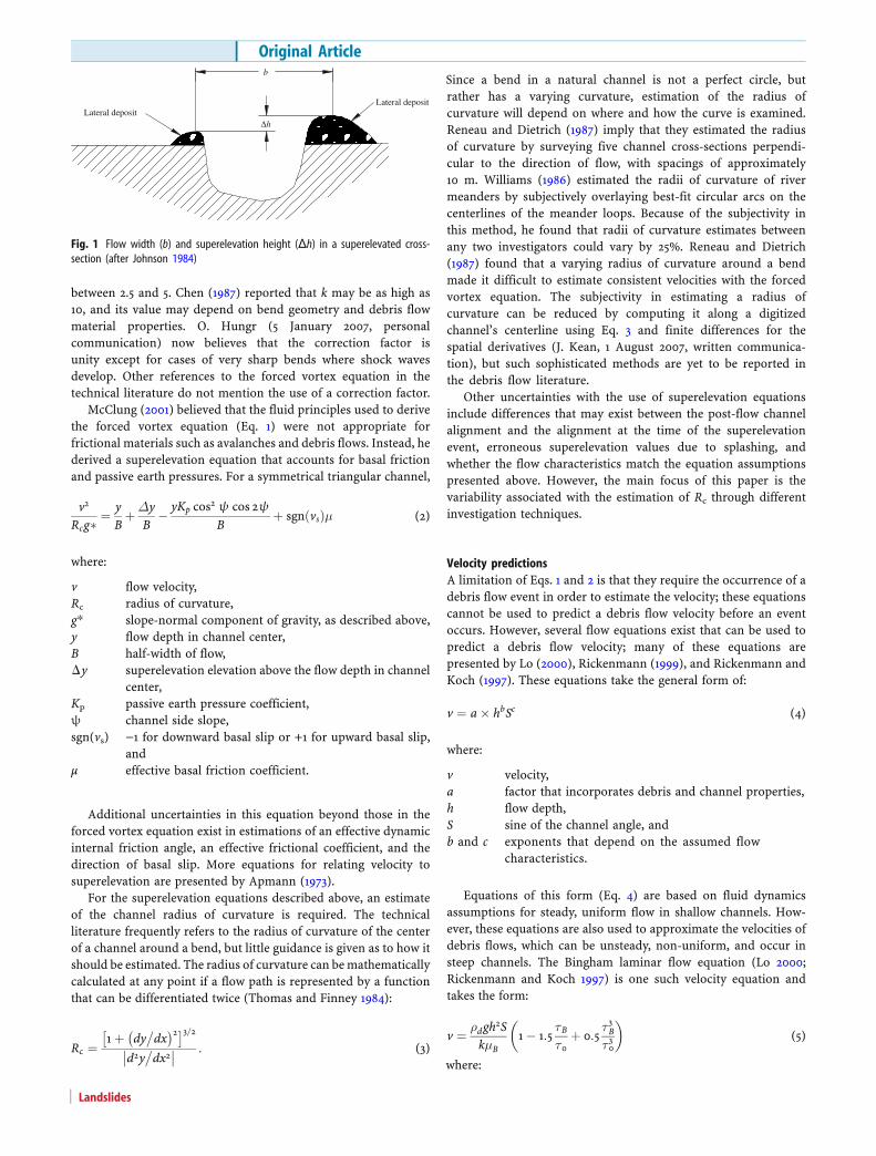
v mean flow velocity,Rc the channel’s radius of curvature,g acceleration of gravity,Δh superelevation height (Fig. 1),k correction factor for viscosity and vertical sorting, andb the flow width (Fig. 1).

The banking angle (β) can be measured instead of measuring band Δh, where β = tan (Δh/b). In order to account for the slope-normal component of gravity, g should be replaced with g* if thechannel slope is greater than 15°, where g*=gcosθ, and θ is the

channel slope (Johnson 1984).

Equation 1 assumes that flow is subcritical, the radius ofcurvature is equal for all streamlines, and every streamline’svelocity is equal to the mean flow velocity (Pierson 1985).Equation 1 was originally derived for water, and thus, thecorrection factor k is sometimes applied to account for theviscosity and vertical sorting of particles within debris flows(Hungr et al. 1984). Different studies suggest different values fork in order to match experimental superelevations to theoreticalvalues. Suwa and Yamakoshi (2000) mention that k is usuallygreater than or equal to 1. VanDine (1996) stated that k may varybetween 1 and 5. Hungr et al. (1984) reported that k may vary

Original Article

Landslides

between 2.5 and 5. Chen (1987) reported that k may be as high as10, and its value may depend on bend geometry and debris flowmaterial properties. O. Hungr (5 January 2007, personalcommunication) now believes that the correction factor isunity except for cases of very sharp bends where shock wavesdevelop. Other references to the forced vortex equation in thetechnical literature do not mention the use of a correction factor.

McClung (2001) believed that the fluid principles used to derivethe forced vortex equation (Eq. 1) were not appropriate forfrictional materials such as avalanches and debris flows. Instead, hederived a superelevation equation that accounts for basal frictionand passive earth pressures. For a symmetrical triangular channel,

v2

Rcg� ¼ yBþΔy

B� yKp cos2 ψ cos 2ψ

Bþ sgn vsð Þμ (2)

where:

v flow velocity,Rc radius of curvature,g* slope-normal component of gravity, as described above,y flow depth in channel center,B half-width of flow,Δy superelevation elevation above the flow depth in channel

center,Kp passive earth pressure coefficient,ψ channel side slope,sgn(vs) −1 for downward basal slip or +1 for upward basal slip,

andμ effective basal friction coefficient.

Additional uncertainties in this equation beyond those in theforced vortex equation exist in estimations of an effective dynamicinternal friction angle, an effective frictional coefficient, and thedirection of basal slip. More equations for relating velocity tosuperelevation are presented by Apmann (1973).

For the superelevation equations described above, an estimateof the channel radius of curvature is required. The technicalliterature frequently refers to the radius of curvature of the centerof a channel around a bend, but little guidance is given as to how itshould be estimated. The radius of curvature can bemathematicallycalculated at any point if a flow path is represented by a functionthat can be differentiated twice (Thomas and Finney 1984):

Rc ¼1þ dy

�dx

� �2� �3=2d2y

�dx2

�� �� : (3)

Since a bend in a natural channel is not a perfect circle, butrather has a varying curvature, estimation of the radius ofcurvature will depend on where and how the curve is examined.Reneau and Dietrich (1987) imply that they estimated the radiusof curvature by surveying five channel cross-sections perpendi-cular to the direction of flow, with spacings of approximately10 m. Williams (1986) estimated the radii of curvature of rivermeanders by subjectively overlaying best-fit circular arcs on thecenterlines of the meander loops. Because of the subjectivity inthis method, he found that radii of curvature estimates betweenany two investigators could vary by 25%. Reneau and Dietrich(1987) found that a varying radius of curvature around a bendmade it difficult to estimate consistent velocities with the forcedvortex equation. The subjectivity in estimating a radius ofcurvature can be reduced by computing it along a digitizedchannel’s centerline using Eq. 3 and finite differences for thespatial derivatives (J. Kean, 1 August 2007, written communica-tion), but such sophisticated methods are yet to be reported inthe debris flow literature.

Other uncertainties with the use of superelevation equationsinclude differences that may exist between the post-flow channelalignment and the alignment at the time of the superelevationevent, erroneous superelevation values due to splashing, andwhether the flow characteristics match the equation assumptionspresented above. However, the main focus of this paper is thevariability associated with the estimation of Rc through differentinvestigation techniques.

Velocity predictionsA limitation of Eqs. 1 and 2 is that they require the occurrence of adebris flow event in order to estimate the velocity; these equationscannot be used to predict a debris flow velocity before an eventoccurs. However, several flow equations exist that can be used topredict a debris flow velocity; many of these equations arepresented by Lo (2000), Rickenmann (1999), and Rickenmann andKoch (1997). These equations take the general form of:

v ¼ a� hbSc (4)

where:

v velocity,a factor that incorporates debris and channel properties,h flow depth,S sine of the channel angle, andb and c exponents that depend on the assumed flow

characteristics.

Equations of this form (Eq. 4) are based on fluid dynamicsassumptions for steady, uniform flow in shallow channels. How-ever, these equations are also used to approximate the velocities ofdebris flows, which can be unsteady, non-uniform, and occur insteep channels. The Bingham laminar flow equation (Lo 2000;Rickenmann and Koch 1997) is one such velocity equation andtakes the form:

v ¼ ρdgh2S

kμB1� 1:5

τBτ0

þ 0:5τ 3Bτ 30

(5)

where:

Δh

b

Lateral depositLateral deposit

Fig. 1 Flow width (b) and superelevation height (Δh) in a superelevated cross-section (after Johnson 1984)

Original Article

Landslides

ρd debris density,g acceleration of gravity,h and S as defined in Eq. 4,k 3 for a wide rectangular channel, 5 for a trapezoidal

channel, and 8 for a semicircular channel,μB Bingham viscosity,τB Bingham yield stress, andτ0 basal shear stress.

Some researchers believe that because of the complexity ofdebris flows in both space and time, their motion cannot berepresented by a single rheological equation (Iverson 2003). Othersadvocate a simple model because of the inherent complexity ofthese flows (O’Brien 1986). Lo (2000) and Rickenmann and Koch(1997) recommend the use of Newtonian turbulent flow equations,but the two sources report using vastly different roughness andfrictional coefficients in order to obtain fits to their datasets. Otherresearchers advocate the use of Bingham models (Johnson 1984),especially for muddy debris flows (O’Brien 1986). The Binghamlaminar flow equation (Eq. 5) is most applicable to flows that can bemodeled as having a yield strength and a linear relationshipbetween shear rate and shear stress (Pierson and Costa 1987).Although inputs to the Bingham flow equation may also be quitevariable (Costa 1984; Iverson 1997) and may not be able toaccurately model the complexity of debris flows (Iverson 2003),simple laboratory tests can be used to estimate these debrisproperties (Johnson and Martosudarmo 1997; Pashias and Boger1996). However, Bingham parameters are dependent on themaximum particle size of the debris flow material that is sampledand tested.

Data sourcesThis study investigated the difficulties associated with both back-calculating and predicting debris flow velocities. Much of the dataused for this study came from field measurements of channelcross-sections (Santi et al. 2006). Channel cross-sections weremeasured using a slope profiler (Gartner 2005; Keaton and DeGraff1996; Santi 1988) following debris flow events from recently burneddrainage basins (Gartner 2005). A slope profiler consists of a woodcrossbar with two legs and an angle finder; the angle finder reportsthe slope of the ground surface between the two legs. By takingsequential angle measurements at a cross-section and trigonome-trically converting the measured angles to x and y coordinates, aprofile of each cross-section was developed. Cross-sections werespaced at 15- to 90-m intervals along the entire channel length. Ateach cross-section, it was also noted which slope profiler intervalscorresponded to levee deposits, muddy veneer deposits, channelincision, bedrock, and the natural slope. The channel slope andazimuth were also recorded for each cross-section.

Topographic maps (1:24,000-scale) and airphotos (1:15,000- and1:8,000-scale) were used to estimate channel radii of curvature atcross-section locations.

Velocity, channel characteristic, and material property datawere obtained from the technical literature to investigate theappropriateness of conventional velocity back-calculation andprediction techniques and also to investigate velocity patternsalong flow paths. Specific data sources are referenced insubsequent sections and are summarized in Table 1. This datasummary suggests that debris flow events analyzed within the

technical literature are primarily large events, and thus, the datasetmay be biased towards higher (more conservative) velocities.

Field estimations of Rc

MethodsTo estimate the ease with which a bend’s radius of curvature can beapproximated in the field, an investigation was performed along achannel bend with superelevated debris flow deposits in KroegerCanyon, Durango, Colorado (Gartner 2005). Eight cross-sectionswere measured around the bend at approximately 6-m spacings. Ateach cross-section, the azimuth normal to the channel orientationwas measured. Multiple radii of curvature were calculated betweenvarious pairs of cross-sections by relating arc lengths to theincluded angles:

L ¼ 2πRc � θ360

(6a)

Rc ¼ 360L2πθ

(6b)

where:

Rc radius of curvature,L channel length (arc length) between the two cross-section,

andθ angular difference (degrees) between the two cross-section

azimuths.

Radii of curvature between different sections were calculatedwith Eq. 6b using channel lengths between 6 and 42 m.

ResultsThe calculated radii of curvature versus the spacings between thecross-sections are shown in Fig. 2. Positive and negative radiicorrespond to clockwise and counterclockwise curvature, respec-tively. The analyzed arc length represents the channel lengthbetween the pair of analyzed cross-sections. Multiple data pointswere obtained for each analyzed arc length by investigating pairs ofcross-sections at different positions around the bend. Differentanalyzed arc lengths were obtained by skipping cross-sectionsbetween those used in the investigated pair.

DiscussionAs the analyzed arc lengths in Fig. 2 increase, the calculated radii ofcurvature begin to stabilize at a consistent value of approximately−100 m (counterclockwise curvature with Rc=100 m). However,considerable scatter exists between the radii of curvaturecalculated from arc lengths shorter than approximately 25 m.Scatter exists for each given arc length, which indicates that theestimation of the radii of curvature is dependent upon the locationalong the arc at which it is measured. Estimated radii of curvaturewere both positive and negative (clockwise and counterclockwisecurvature, respectively), which indicates that this estimationmethod is very sensitive to the measured azimuths of the cross-sections. It appears as if a field investigation method concentrateson local channel irregularities and does not allow for the observerto get a good overall picture of the curve, as an airphoto or mapwould.

Landslides

Table 1 Summary of data obtained from the technical literature

Reference Event/Location Event notes Data used from reference Data acquisition methodsSupercritical versus subcritical flows (Fig. 10)Arattano et al.(1997)

Moscardo Torrent, Italy 10 events from 1990to 1994

Velocity and flowdepth

Ultrasonic sensors

Jackson et al.(1989)

Cathedral Mountain,British Columbia

29 August 1984(87,000 m3)

Measured channel cross-sections,velocities back-calculatedfrom superelevation

Jan et al. (2000) Jiangjia Gulley, China 8 waves from a debrisflow in 1974

Measured at observation station

Jordan (1994) 14 events in British Columbia Measured channel cross-sections,velocities back-calculated fromsuperelevation

McArdell et al.(2003)

Illgraben torrent, Switzerland 28 June 2000(35,000 m3)

Radar and video analysis

Santi (1988) Layton, Utah 12,000 m3 Measured channel cross-sections,velocities back-calculated fromsuperelevation

Tropeano et al.(2003)

Bioley torrent, Italy 92,000 m3 Measured channel cross-sections,velocities back-calculatedfrom superelevation

Laboratory-measured Bingham properties (Fig. 11)Hamilton andZhang (1997)

Jiang-Jia Gulley, China 47 samples from 9 eventsin 1974 and 1975

Yield strength andviscosity

Laboratory analyses

U.C. Davis flume, California 7 samples Laboratory analysesJohnson andMartosudarmo(1997)

Laboratory-preparedwater/sand andslurry/sand mixtures

15 to 48 % solidsby volume

Rolling-sleeve viscometer

Locat (1997) Canadian clays andclayey silts

HAAKE Rotovisco 12

Soule (2006) Samples of debris-flow depositsfrom Georgetown andGlenwood Springs, Colorado

Tested samples containingparticles up to 25.4 mm(1 in.)

Flume box, rolling-sleeveviscometer, inclined plane,slump test

Field back-calculated Bingham properties (Fig. 11)Bertolo andWieczorek(2005)

Yosemite Valley, California 6 events Yield strength andviscosity

Back-calculated from numericalmodeling

Hungr et al.(1984)

British Columbia andJapanese data

15 events Viscosity Best-fit to velocity – depth datausing Newtonian Laminarflow equation

Johnson (1984) Surprise Canyon, California 500,000 m3 Yield strength Estimated from deposit thicknessand sizes of transported clasts

Jordan (1994) 8 events from westernUnited States, New Zealand,and Philippines

Mean value used whenrange was reported

Yield strength andviscosity

Review of published data

11 events in British Columbia Mean value used whenrange was reported

Yield strength andviscosity

Estimated from deposits andvelocities back-calculatedfrom superelevations

Marina andGiuseppe(2007)

Molise Region, Italy Hypothetical situationsbased on potentialsource areas andthe active alluvial fan

Yield strength andviscosity

Back-calculated from numericalmodeling

Rickenmann andKoch (1997)

Kamikamihori valley,Japan

Yield strength andviscosity

Back-calculated from numericalmodeling

Soule (2006) Georgetown and GlenwoodSprings, Coloradodebris flows

Yield strength Estimated from depositthicknesses

Velocity versus position along flow path (Figs. 12 and 13)Arattano (2003) Moscardo Torrent, Italy 22 June 1996 Velocity Ultrasonic and seismic sensorsBertolo andWieczorek(2005)

Yosemite Valley, California Velocity Back-calculated fromsuperelevation

Curry (1966) Mayflower Gulch, Colorado 18 August 1961(17,000 m3)

Velocity Eyewitness

DeGraff (1997) Pilot Ridge, California 2 January 1997(460 m3)

Velocity Back-calculated from run-upand superelevation

Original Article

Landslides

Figure 3 depicts an example of how both clockwise andcounterclockwise curvatures can be obtained from the same bend.If the observer is within a deeply incised channel and a wide extentof the bend cannot be viewed, the azimuth normal to the flowdirection may be incorrectly referenced from the orientation of thepost-debris-flow stream thalweg. In Fig. 3, cross-sections (XS) 1 and2A are both correctly orientated normal to the flow direction, andanalysis of these cross-sections would accurately provide clockwisecurvature. Cross-section 2B is oriented normal to the thalweg butnot to the flow direction, and analysis of cross-sections 1 and 2Bwould result in a large-radius counterclockwise curvature.

Rc variations for different lengths of channel bends

MethodsAlthough the radius of curvature at the point of superelevation(apex of the bend) is required, circle overlaying techniques cannot

be used to identify the radius at a single point. Instead, the radiusmust be estimated by examining the curvature of a length of thechannel. To investigate how estimated radii of curvature varied asthe examined lengths of channel bends changed, radii weremeasured on 1:24,000-scale topographic maps image-referencedinto AutoCAD. Radii were measured on circular arcs fit to sets ofpoints marked on the bend. The first marked point was at alocation of maximum curvature within the debris-flow-producingchannels. Points were also placed 30, 60, and 90 m upstream anddownstream of the points of maximum curvature.

AutoCAD’s drawing function was used to place circles throughthree points: the point ofmaximum curvature and one point on eitherside of it spaced at 30, 60, or 90 m. The radii of curvature for eachcircle were identified by viewing the circle properties. The followingbasins were investigated: tributaries 2, 3, 4, 5, and 6 from Santaquin,Utah (Gartner 2005; McDonald and Giraud 2002) and Kroeger andWoodard Canyons from Durango, Colorado (Gartner 2005).

Reference Event/Location Event notes Data used from reference Data acquisition methodsJackson (1979);Jackson et al.(1989)

Cathedral Mountain,British Columbia

6 September 1978(136,000 m3)

Velocity Eyewitness

Jackson et al.(1989)

Cathedral Mountain,British Columbia

29 August 1984(87,000 m3)

Positions of 5velocity estimates

Back-calculated fromsuperelevations

Jakob et al.(1997)

Pierce Creek and HopeCreek, British Columbia

November 1995(63,000 and 50,000 m3)

Velocity Back-calculated fromsuperelevations

Jakob et al.(2000)

Hummingbird Creek,British Columbia

11 July 1997(92,000 m3)

Positions of 9velocity estimates

Back-calculated fromsuperelevations

Johnson (1984) Surprise Canyon, California 500,000 m3 Velocity Back-calculated fromsuperelevation

Meyer andWells (1997)

Twelve Kilometer, Wyoming 9 July 1989(8,500–14,800 m3)

Velocity Back-calculated from run-up

Meyer et al.(2001)

Jughead Creek, Idaho January 1997(14,600 m3)

Velocity Back-calculated from run-upand superelevation

Nasmith andMercer (1979)

Gulley #1, Port Alice,British Columbia

15 December 1973(22,000 m3)

Velocity Eyewitness

Santi (1988) Layton, Utah 12,000 m3 Positions of 7velocity estimates

Back-calculated fromsuperelevations

h2S versus position along the flow path (Fig. 14 and Table 2)Gartner 2005 Tributary 2, Santaquin, Utah 3,700 m3 Flow depth and channel

slopeSlope-profiler measurementsof channel cross-sectionsTributary 3, Santaquin, Utah 6,200 m3

Tributary 4, Santaquin, Utah 7,000 m3

Tributary 5, Santaquin, Utah 3,000 m3

Tributary 6, Santaquin, Utah 5,300 m3

Elkhorn, Durango, Colorado 5,300 m3

Kroeger, Durango, Colorado 15,800 m3

Woodard, Durango, Colorado 6,500 m3

Devore, southern California 22,500 m3

El Capitan I, southern California 450 m3

Lytle Creek W, southernCalifornia

10,400 m3

Waterman N North, southernCalifornia

204,000 m3

Water Tank, southernCalifornia

2,200 m3

Velocity versus h2S (Fig. 15)Jackson et al.(1989)

Cathedral Mountain,British Columbia

29 August 1984(87,000 m3)

Velocity, flow depth, andchannel slope

Measured channel cross-sections,velocities back-calculated fromsuperelevationJordan (1994) 14 events in British Columbia

Santi (1988) Layton, Utah 12,000 m3

Tropeano et al.(2003)

Bioley torrent, Italy 92,000 m3

Table1 (continued)

Landslides

In addition to estimating radii of curvature from a circle fit tothree points, the use of a second-order polynomial was alsoinvestigated. The coordinates of the three points along the bendswere identified using AutoCAD, and second-order polynomialswere fit to these points. The polynomials were differentiated twiceand radii of curvature were calculated using Eq. 3.

ResultsFigure 4 depicts an example of how a bend’s radius of curvature, asestimated by a circle fit to three points along the channel, changesas the investigated length of the channel changes.

A summary of all the analyzed cross-sections is presented inFig. 5. In Fig. 5, the y-axis depicts the radii of curvature calculatedfrom a circle with 60 or 90-m point spacings normalized by(divided by) the radii of curvature obtained from a circle when 30-m point spacings were used.

DiscussionFigure 5 shows that larger radii of curvature resulted when longerextents of curves were examined. This phenomenon is magnified for

tighter bends. Thus, an estimated radius of curvature for a naturalchannel will depend upon what extent of the bend is examined. Asthe examined length of channel decreases, the estimated radius willapproach that for the singular point of superelevation. Therefore, toanalyze the shortest possible channel length, the largest scale, highestresolution media available should be used.

It appears that for radii of curvature greater than approximately200 m, or more than twice the largest point spacing of 90 m, lessdependence on point spacing is shown. However, radii of curvatureused to back-calculate velocities reported in the technical literatureare typically less than 100 m (Bertolo and Wieczorek 2005; Chou etal. 2000; Cui et al. 2005; Jackson et al. 1989; Jakob et al. 1997;Johnson 1984; Jordan 1994; Santi 1988).

For this study, the arbitrary point spacings of 30, 60, and 90 mwere chosen to systematically analyze the changes in estimatedradii for various curves as the analyzed curve segments increased.In practice, judgment would be required to select the locations ofrepresentative points on a case-by-case basis.

The calculation of radii of curvature from polynomials wasimpractical. The accuracy of the differentiation procedure washighly dependent upon the number of significant figures within thepolynomial coefficients. In order to obtain realistic radii from Eq. 3,more accuracy was required than could reasonably be expectedfrom 1:24,000-scale topographic maps.

Fig. 3 Example of how clockwise and counterclockwise curvature can bemeasured from the same bend

100 m

North

Channel Alignment

Rc = 149 m

for 3 points spaced at 90 m

Rc = 100 m

for 3 points spaced at 60 m

Rc = 50 m

for 3 points spaced at 30 m

Fig. 4 Example of how a calculated radius of curvature changes as theinvestigated extent of the channel changes

0.0

1.0

2.0

3.0

4.0

5.0

6.0

0 50 100 150 200 250

R c (m) obtained from 3 points spaced at 30 meters

No

rma

lize

d R

c

(Rc from 60-m point spacings)/(Rc from 30-m point spacings)

(Rc from 90-m point spacings)/(Rc from 30-m point spacings)

Fig. 5 Normalized calculated radii of curvature from a fitted circle versus the radiiof curvature calculated from a circle fit to three points spaced at 30 m

-600

-400

-200

0

200

400

600

800

0 6 12 18 24 30 36 42 48

Analyzed Arc Length (m)

Cal

cula

ted

Rc (

m)

Fig. 2 Calculated Rc versus the analyzed length of arc

Original Article

Landslides

Rc variations with different scales of investigated media

MethodsTo investigate how radii of curvature varied for different scales ofinvestigated media, a debris flow in Layton, Utah (Santi 1988) wasanalyzed using a 1:24,000-scale topographic map and 1:15,000-scaleand 1:8,000-scale airphotos. The following cross-sections fromSanti (1988) were examined: 3, 13, 15, 18, 28, and 35. The map andairphotos were image-referenced into AutoCAD. At each cross-section location, circles were overlaid upon the channel in radiiincrements of 15 m in order to estimate the maximum andminimum probable radii of curvature. The radius of curvature foreach cross-section was taken as the average of the maximum andminimum. This process was repeated using all three scales ofmedia.

ResultsFigure 6 shows an example of the maximum and minimum radii ofcurvature estimated for cross-sections 13, 15, and 18 of the Layton,Utah debris flow (Santi 1988). The same aerial extent is presentedon the three media shown in Fig. 6, and the displayed media areproportional to their original scales.

A summary of all the data is presented in Fig. 7. In Fig. 7, the y-axis depicts the average radii of curvature estimated from different

scale media normalized by the radii estimated from the 1:8,000-scale airphoto.

DiscussionFigure 7 shows that larger radii of curvature resulted from usingsmaller scale media. This phenomenon is magnified for tighterbends. Thus, an estimated radius of curvature for a natural channelwill depend upon the scale of media used for its estimation. Toobtain the best definition of a bend’s radius of curvature, thelargest scale, highest resolution media available should be used.

Variations in back-calculated velocity at different locationsalong a channel

MethodsIn order to investigate the consistency of velocities back-calculatedby Eq. 1 at various locations within a reach of channel, velocitieswere back-calculated from 21 cross-sections along tributary 5 inSantaquin, Utah (McDonald and Giraud 2002). The cross-sectionlocations are shown in Fig. 8.

At each cross-section location, circles were overlaid upon thechannel in radii increments of 15 m in order to estimate themaximum and minimum probable radii of curvature. The super-elevation height and flow width were obtained from slope profilermeasurements of each cross-section. The position of the debrisflow surface at each cross-section was estimated based on eitherdeposit or scour. At cross-sections that had levees or muddy veneerdeposits on both sides of the channel, the surface of the flow wasassumed to have extended linearly between the two deposits. Atcross-sections that did not have debris flow deposits, the surface ofthe flow was assumed to have extended linearly between thehighest debris flow scour on each side of the channel.

Due to the fact that the highest positions of deposit or scourmay not necessarily coincide with x, y coordinates of the slope-profiler-obtained cross-sections, reasonable error ranges wereapplied to the cross-sections based on the expected accuracy of themeasurement method. Error ranges of ±0.3 m were applied to themeasured flow widths and ±0.1 m were applied to the bank heights.At each cross-section, Eq. 1 (with k=1) was used with the identifiedranges of radii of curvature, bank height, and flow width tocalculate a range of velocities.

Fig. 6 Examples of maximum and minimum radii of curvature identified using a1:24,000 USGS Quadrangle map (a), a 1:15,000 airphoto (b), and a 1:8,000airphoto (c) for cross-sections 13 (red), 15 (yellow), and 18 (green, Santi 1988)

0.0

0.5

1.0

1.5

2.0

2.5

3.0

3.5

4.0

0 20 40 60 80 100 120 140

Average R c from 1:8,000-scale airphoto (m)

No

rmalized

Avera

ge R

c

(1:15k Rc)/(1:8k Rc)

(1:24k Rc)/(1:8k Rc)

Fig. 7 Normalized average radii of curvature versus average radii of curvatureestimated from the 1:8,000-scale airphoto

Landslides

ResultsFigure 9 shows the calculated ranges of velocities for each of thecross-sections shown in Fig. 8. The data points in the interiors ofthe error bars represent the velocities calculated using themeasured bank heights and flow widths and the mean radii ofcurvature for each cross-section. The extents of the error barsrepresent the velocities calculated when the error ranges discussedabove were applied to the flow widths and bank heights, and radiiof curvature were varied between the maximum and minimumones identified for each cross-section. Negative velocities arereported for cross-sections where scour or deposits were higher onthe inside of the curve. This occurrence is explained in thefollowing section.

DiscussionFigure 9 shows that a back-calculated velocity is dependent uponthe analyzed location within a channel. Although many cross-sections consistently produced back-calculated velocities in therange of 5 to 15 m/s, others resulted in velocities less than 5 m/s.Taking into account the velocity ranges indicated by the error bars

and also the variations between different locations along this reachof channel, a large range of velocities could conceivably be back-calculated from this event.

The anomalously high velocities in Fig. 9 may be attributed tosplashing on the outside of a bend; splash marks may have beenincorrectly identified as the maximum height of the flow. Thepresence of deposits being higher on the inside of the bend may beattributed to flow momentum inherited from upstream andinteraction with the walls of the bend. In a non-uniform bend,flow may strike the outside wall of the channel and reflect back tothe inside rather than gradually superelevating around the bend (T.C. Pierson, 11 December 2006, personal communication).

The presence of deposits being higher on the inside of the bendmay also be attributed to supercritical flow. During supercritical flow,superelevation effects can be cancelled if a maximum cross-waveheight occurs on the inside of the bend (Pierson 1985). Figure 10shows a plot of flow velocity versus flow depth for several debrisflows. These data were obtained from velocities and correspondingflow depths published by Arattano et al. (1997), Jackson et al. (1989),Jan et al. (2000), Jordan (1994), McArdell et al. (2003), Santi (1988),and Tropeano et al. (2003).

Figure 10 shows that many combinations of debris flow depthand velocity from the technical literature indicate supercritical flowconditions. The forced vortex equation (Eq. 1) assumes subcriticalflow (Chow 1959). In order to back-calculate a velocity fromsupercritical flow, a single cross-section cannot be analyzed.Rather, the effective superelevation height must be measuredbetween inside and outside cross-wave maxima (Pierson 1985).

Lab versus field material properties

MethodsA database of Bingham properties (viscosity and yield strength)was developed from data in the technical literature to investigatethe feasibility of using laboratory-measured rheological propertiesfor debris flow velocity predictions in equations such as Eq. 5. Datawere divided into two groups: those measured from laboratorytests and those back-calculated from field debris flow events.Laboratory-measured data were obtained from Hamilton andZhang (1997), Johnson and Martosudarmo (1997), Locat (1997),and Soule (2006). Back-calculated values from field events were

Fig. 8 Locations of cross-sections 15 through 52 in Tributary 5, Santaquin, Utah(McDonald and Giraud 2002)

-25

-20

-15

-10

-5

0

5

10

15

20

25

0 400 800 1200 1600

Distance upstream (m)

Ve

loc

ity (

m/s

)

Bank based on deposit

Bank based on scour

XS 15

XS 52

Fig. 9 Back-calculated velocities for cross-sections 15 through 52 in Tributary 5,Santaquin, Utah (McDonald and Giraud 2002). Negative velocities are reported forcross-sections where scour or deposits were higher on the inside of the curve

0

3

6

9

12

15

0 2 4 6 8 10

Flow Depth, h (m)

Velo

city (

m/s

)

Superelevation Analysesfrom this study

Superelevation Analysesfrom Literature

Other velocity estimatesfrom Literature

Subcritical Flow

Fr < 1

Supercritical Flow

Fr > 1

Fig. 10 Debris flow velocity versus flow depth. Many combinations indicatesupercritical flow

Original Article

Landslides

obtained from Bertolo and Wieczorek (2005), Hungr et al. (1984),Johnson (1984), Jordan (1994), Marina and Giuseppe (2007),Rickenmann and Koch (1997), and Soule (2006).

ResultsA plot of Bingham properties (viscosity and yield strength)obtained from laboratory tests and back-calculated from fielddebris flow events is shown in Fig. 11. Field values that are plottedalong each axis did not have corresponding values of the otherproperty reported. Individual data points from Soule (2006) weretoo numerous to plot, but the extents of his data are represented bythe outlined rectangle.

DiscussionFigure 11 shows that two distinct populations of Binghamproperties exist between those measured from laboratory testsand those back-calculated from field events. Yield strengths back-calculated from field events vary by nearly an order of magnitudeon either side of the generalized estimate of 3,000 Pa*s of Hungret al. (1984). Higher apparent Bingham properties obtained fromfield events are presumably due to large-particle frictionalinteractions, which cannot be measured in laboratory-scalespecimens. The presence of this frictional resistance indicatesthat the back-calculated field events would be more appropriatelyrepresented by a Coulomb frictional model than a Bingham model(Iverson 2003) and confirms Major and Iverson’s (1999) belief thatdebris strength cannot be inferred from deposit thickness. Sincelaboratory-obtained rheological properties are not representativeof field-scale debris flow behavior, these values could not be usedfor velocity predictions. It may be possible to use apparentBingham properties calibrated from field-scale events to predictthe velocities of similar events, although a Binghammodel may notbe the most physically accurate choice.

Flow trends within channels

MethodsA database of estimated debris flow velocities at different positionswithin channels was developed from the technical literature. Datawere obtained from the following sources: Arattano (2003), Bertoloand Wieczorek (2005), Curry (1966), DeGraff (1997), Jackson

(1979), Jackson et al. (1989), Jakob et al. (1997, 2000), Johnson(1984), Meyer and Wells (1997), Meyer et al. (2001), Nasmith andMercer (1979), and Santi (1988). Debris flow velocity was plottedversus the distance upstream of the fan for each data point.

Much of these velocity data, and other data that will be used inthe subsequent section, were back-calculations from supereleva-tions by the original investigators. Although this paper hasreported several difficulties with the back-calculation of velocitiesfrom superelevations, these are the best data available. Thesevelocities fall within the typical range for debris flows as defined byLorenzini and Mazza (2004) and are also within the range of debrisflow velocities obtained by more certain methods such asinstrumentation (e.g., Arattano and Grattoni 2000; Genevois etal. 2000; Suwa et al. 2003), video surveillance (e.g., Arattano andGrattoni 2000; Genevois et al. 2000; Zhang and Chen 2003), oreyewitnesses (e.g., Hungr et al. 1984; Jackson 1979). Flow depthsreported within the original references indicate that approximatelyhalf of these velocity data were collected from subcritical flows.

Based on the form of Eq. 4, channel slope and flow depth wereidentified as being two easily measured factors expected tocorrelate to measured velocity. The channel slope and flow depthwere identified for each measured cross-section in several of theexamined basins that produced fire-related debris flows. Thebasins used for analysis were tributaries 2, 3, 4, 5, and 6 in Utah(Gartner 2005; McDonald and Giraud 2002); Elkhorn, Kroeger, andWoodard in Colorado (Gartner 2005); and Devore, El Capitan I,Lytle Creek W, Waterman N North, and Water Tank in California(Gartner 2005). The data obtained from these basins (Gartner2005) do not allow for the differentiation between instantaneousflow depths and the maximum depth of scour. Thus, the flow depthused for this analysis was the depth from the top of debris flowscour or deposit to the bottom of the scoured channel, which maybe greater than any instantaneous flow depth. For each basin, thevalue h2S at each cross-section was analyzed versus the distanceupstream of the fan, where h is the flow depth and S is the sine of thechannel slope. The decision to use h2S was based on empirical data,which will be shown in a subsequent section. However, theseexponential powers of flow depth and channel slope are identical tothose used in Newtonian laminar flow and Bingham laminar flowequations (Lo 2000) and are also proportional to the shear forcewithin a steady, uniform, viscous flow (Savage and Smith 1986).

ResultsVelocity estimates had been made at numerous points along thetravel path for three debris flow events in the literature: CathedralGulch 1984 (Jackson et al. 1989), Hummingbird Creek (Jakob et al.2000), and Layton, Utah (Santi 1988). Velocity trends for thesethree events are shown in Fig. 12. The trends for these three eventsshow that velocities were generally consistent along the length ofthe channel.

Figure 13 shows a plot of all the data from the technicalliterature for estimated debris flow velocities versus the distanceupstream of the alluvial fan. These data include those from Fig. 12in addition to data from debris flows for which only one or twovelocity measurements were made. These data show that a widerrange of velocities have been reported near alluvial fans thanfarther upstream in channels.

The h2S data measured from fire-related debris flows (Santi etal. 2006) were statistically analyzed for any trends along the lengthsof the debris flow paths. Figure 14 shows an example of h2S values

0.001

0.01

0.1

1

10

100

1000

10000

100000

0.001 0.01 0.1 1 10 100 1000 10000

Viscosity (Pa*s)

Yie

ld S

tren

gth

(P

a)

Calibrated and Back-calculated from field studies

Measured from lab tests

Range of lab test results from Soule (2006)

Viscosity values with no

corresponding yield

strength reported

Yield Strength values with

no corresponding viscosity

reported

Fig. 11 Bingham properties (viscosity and yield strength) obtained fromlaboratory tests and field back-calculations

Landslides

from each cross-section of Lytle Creek W, along with their mean,standard deviation, and regression results. A summary of thesedata from all the analyzed basins is shown in Table 2. Also shown inTable 2 are the P values obtained from regressions of h2S versusdistance upstream for each analyzed basin.

DiscussionThe results in Fig. 12 show that velocities were approximatelyconstant along the length of the flow path for the three eventsshown. Although some data points show localized deviations,velocity is generally consistent along these flow paths. These resultscontradict Pierson (1985) who found that velocities decreasedalong the lengths of flow paths for the Pine Creek and Muddy Riverlahars. Comparing these lahars to the events shown in Fig. 12 wouldbe questionable, though, due to the larger magnitude (1.4×107 m3)and initiation mode (pyroclastic surge) of the lahars.

The results in Fig. 12, which show uniform velocities along flowpaths, were obtained from a few choice locations along thechannel. The results in Fig. 9, which show a wide range of back-calculated velocities along the flow path, were obtained from amuch denser sampling of bends along the channel length.Therefore, not all channel bends will be appropriate for super-

elevation calculations, and care must be taken when choosingbends to analyze.

Figure 13 shows that for all the data from the technical literature,a wider range of velocities are reported near alluvial fans thanfarther upstream in channels. We interpret this not to mean thatvelocities become more variable near alluvial fans, but rather that awider range of events have been examined near the mouths ofchannels. In Fig. 13, data presented within the first 500 m from thefan were obtained from 14 different debris flow events, while datapresented greater than 500 m from the fan were obtained from onlysix different events reported by five sources. The wide range ofvelocities reported near the fan in Fig. 13 may also be caused bydecreasing velocities due to deposition or the inconsistency ofvelocity estimation methods.

The high P values on the regressions in Table 2 indicate that forall but two basins, the regressions are not statistically significant ata significance level of 0.05. Therefore, it would be concluded thatthe mean is just as good a predictor of h2S as is the regression, andh2S is constant along the travel path. This is caused by thesimultaneous decrease in channel slope along the flow path asbulked material increases the flow depth. For the two basins withstatistically significant regressions (tributary 2 and Woodard), thepractical significance of these regressions will be discussed in asubsequent section.

The data from the basins listed in Table 2 were obtainedprimarily from modest-sized debris flow events, with magnitudesless than 20,000 m3 (size classes 3 and 4, Jakob 2005). For everyevent other than Devore, the mean h2S value was less than or equalto 2.5 m2, and the channel had been scoured to bedrock over muchof its length. The magnitude of this h2S value will be put intoperspective in a subsequent section. The constancy of h2S valuesalong the travel paths of these fire-related debris flows is attributedto the presence of shallow bedrock, which limits the potentialdepth of scour. Thus, the event volume, peak flow, and flow depthare also finite.

Devore was the only analyzed basin with a mean h2S valuegreater than 3 m2. Although no statistically significant trend wasobserved between h2S and the channel position for Devore, thisevent did exhibit highly random h2S values and a high depth offlow overall. We attribute this to the abundance of materialavailable for mobilization within the channel, since Devore Canyon

0

5

10

15

20

25

30

0 500 1000 1500 2000

Distance upstream of the fan (m)

Ve

loc

ity

(m

/s)

Cathedral Gulch, B.C.

Hummingbird Creek, B.C.

Layton, UT

Fig. 12 Debris flow velocity estimations versus distance upstream of the fan forindividual events

0

5

10

15

20

25

30

0 500 1000 1500 2000

Distance upstream of the fan (m)

Ve

loc

ity

(m

/s)

Fig. 13 Debris flow velocity estimations versus distance upstream of the fan

y = -0.0007x + 2.3941

R2 = 0.0577

0

1

2

3

4

5

6

7

8

9

10

0 500 1000 1500 2000

Distance upstream of the fan (m)

h2S

(m

2)

Mean

Mean +/- 1 Standard Deviation

Linear (Lytle W)

Fig. 14 Example of h2S versus distance upstream of the fan for Lytle Creek W(Gartner 2005), where h is the flow depth and S is the sine of the channel angle

Original Article

Landslides

is located near the convergence of several faults (Dibblee 2003a, b).Field observations showed channel incision of up to 2 m intostored colluvium in the channel of Devore Canyon.

We would expect landslide-initiated debris flows to showsimilar trends to the analyzed fire-related flows, but to have higherh2S values due to the volume of the initiating event. Some basins inTable 2 have standard deviations of the h2S values that are largerthan the mean value; this is attributed to the presence of a fewanomalously deeply scoured cross-sections in a channel with anotherwise low mean h2S value.

Since velocity and h2S are both approximately constant alongthe paths of the analyzed debris flows, it may be possible to obtaina preliminary velocity estimate from the channel slope and theexpected depth of flow. This estimated velocity would be applicablealong the entire length of channel.

Velocity versus h2S

MethodsA database was developed from the technical literature forlocations where an estimated velocity, flow depth, and channel

slope were all reported. Data were obtained from the followingsources: Jackson et al. (1989), Jordan (1994), Santi (1988), andTropeano et al. (2003). These data are from landslide-initiateddebris flows in British Columbia, Utah, and Italy. Although thesevelocities were back-calculated from superelevations, we againconsider them valid for the same reasons presented in the previoussection. Statistical analyses were performed to correlate velocity toh2S. A larger dataset would have been desirable, but reports in thetechnical literature of debris flow velocity, flow depth, and channelslope at a single location were rare.

ResultsFigure 15 shows a plot of velocity versus h2S, along with the best-fitregression line to the data. The standard errors of the regressionline’s slope and intercept are 0.06 and 0.61, respectively. Theresiduals from this regression are homoscedastic and the normalprobability plot of the residuals is reasonably linear. The verticallines in Fig. 15 divide the data into three near-equal subsets at h2Svalues of 3 and 6 m2. The statistical distribution of the data withineach subset is summarized in Table 3.

DiscussionThe R2 value in Fig. 15 shows that h2S explains approximately halfof the scatter within the dataset. The other half of the scatter islikely due to differences in material properties and channelcharacteristics between the events in the dataset. These additionalfactors (coefficient a from Eq. 4) are approximately incorporated intothe slope of the best-fit regression line shown in Fig. 15, which are toovaried and difficult to characterize and quantify to justify attempts to

Table 3 Summary of velocity versus h2S data

h2S<3 m2

(m/s)3 m2<h2S<6 m2

(m/s)6 m2<h2S(m/s)

Mean−1 SD 3.7 4.5 7.0Mean 6.0 6.8 10.4Mean+1 SD 8.3 9.1 13.8Mean+2 SD 10.6 11.4 17.2

Table 2 Summary of h2S versus upstream distance data for all analyzed basins

Regression results P valuesBasin Mean of h2S

(m2)Standard deviation ofh2S (m2)

Slope (m) ×10−5

Slope SE (m)×10−5

Intercept(m2)

Intercept SEa

(m2)Intercept Regression Number Channel

length (m)Tributary 2 0.87 0.92 55 17 0.18 0.24 0.46 0.00 63 2,300Tributary 3 0.72 0.80 16 9.4 0.45 0.18 0.02 0.09 73 3,400Tributary 4 0.67 0.95 7.0 12 0.56 0.22 0.02 0.56 68 3,200Tributary 5 1.7 1.8 −74 57 2.3 0.53 0.00 0.20 46 1,500Tributary 6 0.85 0.88 22 18 0.59 0.24 0.02 0.21 51 2,400Elkhorn 2.5 3.5 −260 140 4.2 1.1 0.00 0.07 41 1,300Kroeger 0.19 0.18 −4.2 3.3 0.25 0.06 0.00 0.21 41 3,000Woodard 1.0 2.4 −190 56 3.2 0.71 0.00 0.00 48 2,000Devore 4.6 3.3 120 110 3.8 0.87 0.00 0.29 47 1,400El Capitan I 1.4 1.1 −39 84 1.56 0.44 0.00 0.64 29 890Lytle CreekW

1.8 1.4 −74 45 2.4 0.42 0.00 0.11 46 1,600

Waterman NNorth

0.60 0.49 −99 66 0.95 0.26 0.00 0.16 17 600

Water tank 2.1 2.3 490 410 0.84 1.1 0.47 0.25 21 430

SE standard error

y = 0.35x + 5.36

R2 = 0.49

0

2

4

6

8

10

12

14

16

0 5 10 15 20 25 30

h2

S (m2)

Ve

loc

ity (

m/s

)

P value = 0.00

Fig. 15 Velocity versus h2S. Dashed vertical lines are at h2S equal to 3 and 6 m2

Landslides

include them in the correlation to predict a preliminary velocity. Thelow P value indicates that the regression is statistically significant; thevelocities within the dataset do increase with increasing values of h2S,and h2S is a better predictor of velocity than is themean of the dataset.The results summary shown in Table 3 is based on a limited amount ofavailable data, and considerable scatter exists within the data shownin Fig. 15. However, this method shows promise of h2S being apredictor of debris flow velocity (if the velocities back-calculated fromsuperelevations are correct), and it should be tested with additionaldata as they become available.

In comparing the h2S data from Table 2 to the data and analysisreported by Fig. 15 and Table 3, all but one of the analyzed debrisflow events from Table 2 would fall within the lowest category ofTable 3: h2S<3 m2. For the two events that had statisticallysignificant regressions (Table 2, tributary 2 and Woodard),deviations along the channel are still contained within the categoryh2S<3 m2. Devore would fall within the middle category, and noanalyzed events from Table 2 had h2S values larger than 6 m2.

Figure 16 shows the flow depth and channel slope combinationsat the h2S category boundaries shown in Fig. 15 and Table 3.Modest-sized flows will have h2S values less than 3 m2, and onlyvery large flows will have h2S values greater than 6 m2.

A velocity may be estimated from Table 3 for use in preliminarydesigns. A maximum possible flow depth, h, may be estimated asthe height from bedrock to the top of the channel banks. Thisestimate conservatively assumes that during a debris flow, thechannel has been scoured down to bedrock and the channel isflowing full. An increase in flow depth above the height of thechannel banks will cause material to spill over and deposit due tolack of confinement, effectively limiting the maximum potential

flow depth. However, for long-duration debris flows withmultiple surges, the maximum instantaneous flow depth maybe less than this maximum possible depth. Alternatively, the highflow marks from previous debris flows could be used to estimatea flow depth for the prediction of the velocities of similar-sizedevents. This method would be required for deeply incisedcanyons that do not contain channel banks to limit themaximum height of flow.

Combinations of flow depth and channel slope other than h2Swere preliminarily investigated as being predictors of velocity, aswere other channel and material characteristics. Based on dataavailable within the technical literature, h2S was found to producethe highest R2 value of the various combinations of predictors,although other combinations of flow depth and channel slope fitthe velocity data similarly (Table 4). Best-fit regression equationsobtained from other combinations of flow depth and channel slopeare summarized in Table 4.

Summary and conclusionsBack-calculation of velocities for recent debris flows has been shownto be a subjective and problematic process. There is not an absolutevalue of a radius of curvature for a natural channel’s bend, butreasonable approximations may be made. An estimated radius ofcurvature will vary with the extent of the bend investigated and thescale of the media used. Because of their dependence on thismeasurement, back-calculated velocities can vary significantly be-tween different analyzed cross-sections. Another significant diffi-culty with velocity back-calculation is that many debris flow eventsfrom the technical literature would be classified as supercriticalflows. In these instances, the forced vortex equation (Eq. 1) cannotbe applied to an individual cross-section, but rather the super-elevation height must be estimated between inside and outsidecross-wave maxima.

This paper has identified several difficulties with the use of theforced vortex equation. However, the purpose of this paper has onlybeen to disseminate these difficulties, not to denounce the methodentirely. Many experienced researchers have reported back-calcu-lated velocities from superelevations that appear to be reasonable,but the process is not nearly as straightforward as it appears.

Prediction of debris flow velocity at locations where back-calculation is not possible requires information about materialproperties for use in flow equations. We have shown that twopopulations of Bingham properties (viscosity and yield strength)exist between those measured from laboratory samples and thoseback-calculated from field-scale debris flows. This indicates that aBingham model would not be physically appropriate for friction-dominated debris flows, which are flows containing large particles.Therefore, laboratory-obtained properties, which are generallyderived from only the finer fraction of debris samples, should not

0

2

4

6

8

10

0 5 10 15 20 25

Channel Slope (degrees)

Flo

w D

ep

th (

m)

h2

S < 3 m2

6 m2 < h

2S

h2

S = 3 m2

h2

S = 6 m2

Fig. 16 Flow depth and channel slope combinations at the h2S categoryboundaries

Table 4 Analysis results using other combinations of flow depth and channel slope

Flow model Form of flow depth (h) and channel slope (S) Reference Best-fit regression equationa R2

Dilatant h3/2S1/2 Hungr et al. (1984); Lo (2000) v ¼ 0:55 h3=2S1=2� �þ 4:59 0.47

Newtonian turbulent (Manning) h2/3S1/2 Lo (2000); Rickenmann (1999) v ¼ 4:47 h2=3S1=2� �þ 1:71 0.44

Newtonian turbulent (Chézy) h1/2S1/2 Rickenmann (1999) v ¼ 6:53 h1=2S1=2� �þ 1:03 0.37

Empirical h2/3S1/5 Lo (2000) v ¼ 3:32 h2=3S1=5� �þ 0:70 0.47

Empirical h0.3S1/2 Rickenmann (1999) v ¼ 8:90 h0:3S1=2� �þ 1:06 0.24

aWith flow depth in meters and velocity in m/s.

Original Article

Landslides

be used for field-scale velocity predictions. However, reasonablevelocity estimates may be obtained if back-calculated apparentBingham properties are used.

Flow velocity and h2S both tentatively appear to be ratherconsistent along the length of a debris flow path. A preliminarydebris flow velocity prediction can be made from a channel’s slopeand the expected depth of flow by using Table 3, if the back-calculated velocity data presented in Fig. 15 are assumed to becorrect. The maximum depth of flow would extend from bedrockto the loss of confinement at the top of the channel banks.Although the relationship between h2S and velocity is based ononly a modest dataset, it appears to be a worthwhile estimationmethod that avoids the difficulties of other debris flow velocityestimation methods. The validity of this method should continueto be assessed as additional data become available.

AcknowledgmentsThis work has been funded by the US Department of Educationthrough a Graduate Assistance in Areas of National Need(GAANN) Fellowship, award #P200A060133. Thanks to RichardGiraud from the Utah Geological Survey for providing airphotosand to Ron Allingham for AutoCAD assistance. Also thanks toVictor deWolfe, Joe Gartner, Morgan McArthur, and Nate Soule forthe measurement of many of the cross-sections used in this study.Joe Gartner, Jason Kean, and two anonymous reviewers providedhelpful comments on an earlier draft of this paper.

References

Apmann RP (1973) Estimating discharge from superelevation in bends. J Hydraul Div99:65–79

Arattano M (2003) Monitoring the presence of the debris-flow front and its velocitythrough ground vibration detectors. In: Rickenmann D, Chen C-L (eds) Debris-flowhazards mitigation: mechanics, prediction, and assessment. Proceedings of the thirdinternational conference. Millpress, Rotterdam, pp 719–730

Arattano M, Grattoni P (2000) Using a fixed video camera to measure debris-flowsurface velocity. In: Wieczorek GF, Naeser ND (eds) Debris-flow hazards mitigation:mechanics, prediction, and assessment. Proceedings of the second internationalconference. AA Balkema, Rotterdam, pp 273–281

Arattano M, Deganutti AM, Marchi L (1997) Debris flow monitoring activities in aninstrumented watershed on the Italian Alps. In: Chen C-L (ed) Debris-flow hazardsmitigation: mechanics, prediction, and assessment. Proceedings of the firstinternational conference. ASCE, New York, pp 506–515

Bertolo P, Wieczorek GF (2005) Calibration of numerical models for small debris flows inYosemite Valley, California, USA. Nat Hazards Earth Syst Sci 5:993–1001

Chen C-L (1987) Comprehensive review of debris flow modeling concepts in Japan. In:Costa JE, Wieczorek GF (eds) Reviews in engineering geology, vol VII. Debris flows/avalanches: process, recognition, and mitigation. The Geological Society of America,Boulder, CO, pp 13–29

Chou HT, Liao WM, Lin ML (2000) Landslide induced debris-flow at a dump site. In:Wieczorek GF, Naeser ND (eds) Debris-flow hazards mitigation: mechanics, prediction,and assessment. Proceedings of the second international conference. AA Balkema,Rotterdam, pp 157–160

Chow VT (1959) Open-channel hydraulics. McGraw-Hill, New YorkCosta JE (1984) Physical geomorphology of debris flows. In: Costa JE, Fleisher PJ

(eds) Developments and applications of geomorphology. Springer, Berlin, pp268–317

Cui P, Chen X, Waqng Y, Hu K, Li Y (2005) Jiangjia Ravine debris flows in south-westernChina. In: Jakob M, Hungr O (eds) Debris-flow hazards and related phenomena.Praxis, Chichester, pp 565–594

Curry RR (1966) Observation of alpine mudflows in the Tenmile Range, central Colorado.Geol Soc Amer Bull 77:771–776

DeGraff JV (1997) Geologic investigation of the Pilot Ridge debris flow, GrovelandRanger District, Stanislaus National Forest. United States Department of AgricultureForest Service FS-6200-7 (10/73)

Dibblee TW Jr (2003a) Geologic map of the Cajon Quadrangle, San Bernardino County,California. Dibblee geology center map #DF-104. Santa Barbara Museum of NaturalHistory, Santa Barbara, California

Dibblee TW Jr (2003b) Geologic map of the Devore Quadrangle, San Bernardino County,California. Dibblee geology center map #DF-105. Santa Barbara Museum of NaturalHistory, Santa Barbara, California

Gartner JE (2005) Relations between wildfire related debris-flow volumes and basinmorphology, burn severity, material properties and triggering storm rainfall. Masterof Arts thesis, University of Colorado Department of Geography

Genevois R, Tecca PR, Berti M, Simoni A (2000) Debris-flows in the dolomites:experimental data from a monitoring system. In: Wieczorek GF, Naeser ND (eds)Debris-flow hazards mitigation: mechanics, prediction, and assessment. Proceedingsof the second international conference. AA Balkema, Rotterdam, pp 283–291

Hamilton D, Zhang S (1997) Velocity profile assessment for debris flow hazards. In: ChenC-L (ed) Debris-flow hazards mitigation: mechanics, prediction, and assessment.Proceedings of the first international conference. ASCE, New York, pp 474–483

Henderson FM (1966) Open channel flow. Macmillan, New YorkHungr O, Morgan GC, Kellerhals R (1984) Quantitative analysis of debris torrent hazards

for design of remedial measures. Can Geotech J 21:663–677Iverson RM (1997) The physics of debris flows. Rev Geophys 35:245–296Iverson RM (2003) The debris-flow rheology myth. In: Rickenmann D, Chen C-L (eds)

Debris-flow hazards mitigation: mechanics, prediction, and assessment. Proceedingsof the third international conference. Millpress, Rotterdam, pp 303–314

Iverson RM, LaHusen RG, Major JJ, Zimmerman CL (1994) Debris flow against obstaclesand bends: dynamics and deposits. EOS Trans Am Geophys Union 75:274

Jackson LE Jr (1979) A catastrophic glacial outburst flood (jökulhlaup) mechanism fordebris flow generation at the Spiral Tunnels, Kicking Horse River basin, BritishColumbia. Can Geotech J 16:806–813

Jackson LE Jr, Hungr O, Gardner JS, Mackay C (1989) Cathedral Mountain debris flows,Canada. Bull Int Assoc Eng Geol 40:35–54

Jakob M (2005) A size classification for debris flows. Eng Geol 79:151–161Jakob M, Hungr O, Thomson B (1997) Two debris flows with anomalously high

magnitude. In: Chen C-L (ed) Debris-flow hazards mitigation: mechanics, prediction,and assessment. Proceedings of the first international conference. ASCE, New York,pp 382–394

Jakob M, Anderson D, Fuller T, Hungr O, Ayotte D (2000) An unusually large debris flowat Hummingbird Creek, Mara Lake, British Columbia. Can Geotech J 37:1109–1125

Jan CD, Wang YY, Han WL (2000) Resistance reduction of debris-flow due to airentrainment. In: Wieczorek GF, Naeser ND (eds) Debris-flow hazards mitigation:mechanics, prediction, and assessment. Proceedings of the second internationalconference. AA Balkema, Rotterdam, pp 369–372

Johnson AM (1984) Debris flow. In: Brunsden D, Prior DB (eds) Slope instability. Wiley,Chichester, pp 257–361

Johnson AM, Martosudarmo SY (1997) Discrimination between inertial and macro-viscous flows of fine-grained debris with a rolling-sleeve viscometer. In: Chen C-L(ed) Debris-flow hazards mitigation: mechanics, prediction, and assessment.Proceedings of the first international conference. ASCE, New York, pp 229–238

Jordan RP (1994) Debris flows in the Southern Coast Mountains, British Columbia:dynamic behaviour and physical properties. Doctor of Philosophy thesis, TheUniversity of British Columbia

Keaton JR, DeGraff JV (1996) Surface observation and geologic mapping. In: TurnerAK, Schuster RL (eds) Landslides investigation and mitigation. Special Report247, Transportation Research Board, National Research Council, Washington, pp178–230

Lo DOK (2000) Review of natural terrain landslide debris-resisting barrier design. GEOReport No. 104, Geotechnical Engineering Office, Civil Engineering Department, TheGovernment of Hong Kong Special Administrative Region

Locat J (1997) Normalized rheological behaviour of fine muds and their flow propertiesin a pseudoplastic regime. In: Chen C-L (ed) Debris-flow hazards mitigation:mechanics, prediction, and assessment. Proceedings of the first internationalconference. ASCE, New York, pp 260–269

Lorenzini G, Mazza N (2004) Debris flow phenomenology and rheological modeling. WITPress, Southampton

Major JJ, Iverson RM (1999) Debris-flow deposition: effects of pore-fluid pressure andfriction concentrated at flow margins. GSA Bull 111:1424–1434

Marina P, Giuseppe S (2007) The runout of debris flows: application of two numericalmodels and comparison of results. Proceedings of the first North American landslideconference, Vail, Colorado, 3–8 June 2007 (compact disk)

McArdell BW, Zanuttigh B, Lamberti A, Rickenmann D (2003) Systematic comparison ofdebris-flow laws at the Illgraben torrent, Switzerland. In: Rickenmann D, Chen C-L(eds) Debris-flow hazards mitigation: mechanics, prediction, and assessment.Proceedings of the third international conference. Millpress, Rotterdam, pp 647–657

Landslides

McClung DM (2001) Superelevation of flowing avalanches around curved channel bends.J Geophys Res 106:16,489–16,498

McDonald GN, Giraud RE (2002) September 12, 2002, fire-related debris flows east ofSantaquin and Spring Lake, Utah County, Utah. Technical Report 02-09, UtahGeological Survey, Salt Lake City, Utah

Meyer GA, Wells SG (1997) Fire-related sedimentation events on alluvial fans,Yellowstone National Park, U.S.A. J Sediment Res 67:776–791

Meyer GA, Pierce JL, Wood SH, Jull AJT (2001) Fire, storms, and erosional events in theIdaho batholith. Hydrol Process 15:3025–3038

Nasmith HW, Mercer AG (1979) Design of dykes to protect against debris flows at PortAlice, British Columbia. Can Geotech J 16:748–757

O’Brien JS (1986) Physical processes, rheology and modeling of mud flows. Doctor ofPhilosophy dissertation, Colorado State University

Pashias N, Boger DV (1996) A fifty cent rheometer for yield stress measurement. J Rheol40:1179–1189

Pierson TC (1985) Initiation and flow behavior of the 1980 Pine Creek and Muddy Riverlahars, Mount St. Helens, Washington. Geol Soc Amer Bull 96:1056–1069

Pierson TC, Costa JE (1987) A rheologic classification of subaerial sediment-water flows.In: Costa JE, Wieczorek GF (eds) Reviews in engineering geology, vol VII. Debrisflows/avalanches: process, recognition, and mitigation. The Geological Society ofAmerica, Boulder, CO, pp 1–12

Reneau SL, Dietrich WE (1987) The importance of hollows in debris flow studies;examples from Marin County, California. In: Costa JE, Wieczorek GF (eds) Reviews inengineering geology, vol VII. Debris flows/avalanches: process, recognition, andmitigation. The Geological Society of America, Boulder, CO, pp 165–180

Rickenmann D (1999) Empirical relationships for debris flows. Nat Hazards 19:47–77Rickenmann D, Koch T (1997) Comparison of debris flow modelling approaches. In: Chen

C-L (ed) Debris-flow hazards mitigation: mechanics, prediction, and assessment.Proceedings of the first international conference. ASCE, New York, pp 576–585

Santi PM (1988) The kinematics of debris flow transport down a canyon. Master ofScience in Geology Thesis, Texas A&M University

Santi PM, Higgins JD, Cannon SH, DeGraff JV (2006) Evaluation of post-wildfire debrisflow mitigation methods and development of decision-support tools. Final Report tothe Joint Fire Science Program, JFSP Contract 03-1-4-14. Also at http://www.firescience.gov/projects/03-1-4-14/03-1-4-14_final_report.pdf

Savage WZ, Smith WK (1986) A model for the plastic flow of landslides. US Geological SurveyProfessional Paper 1385, United States Government Printing Office, Washington, DC

Soule NC (2006) The influence of coarse material on the yield strength and viscosity of debrisflows. Master of Science in Geological Engineering Thesis, Colorado School of Mines

Suwa H, Yamakoshi T (2000) Estimation of debris-flow motion by field surveys. In:Wieczorek GF, Naeser ND (eds) Debris-flow hazards mitigation: mechanics, prediction,and assessment. Proceedings of the second international conference. AA Balkema,Rotterdam, pp 293–299

Suwa H, Akamatsu J, Nagai Y (2003) Energy radiation by elastic waves from debrisflows. In: Rickenmann D, Chen C-L (eds) Debris-flow hazards mitigation: mechanics,prediction, and assessment. Proceedings of the third international conference.Millpress, Rotterdam, pp 895–904

Thomas GB Jr, Finney RL (1984) Calculus and analytic geometry. Addison-Wesley,Reading, Massachusetts

Tropeano D, Turconi L, Rosso M, Cavallo C (2003) The October 15, 2000 debris flow inthe Bioley torrent, Fenis, Aosta valley, Italy—damage and processes. In: RickenmannD, Chen C-L (eds) Debris-flow hazards mitigation: mechanics, prediction, andassessment. Proceedings of the third international conference. Millpress, Rotterdam,pp 1037–1048

VanDine DF (1985) Debris flows and debris torrents in the Southern Canadian Cordillera.Can Geotech J 22:44–68

VanDine DF (1996) Debris flow control structures for forest engineering. BritishColumbia Ministry of Forests Research Program, Working Paper 08/1996

Williams GP (1986) River meanders and channel size. J Hydrol 88:147–164Zhang S, Chen J (2003) Measurement of debris-flow surface characteristics through

close-range photogrammetry. In: Rickenmann D, Chen C-L (eds) Debris-flow hazardsmitigation: mechanics, prediction, and assessment. Proceedings of the thirdinternational conference. Millpress, Rotterdam, pp 775–784

A. B. Prochaska ()) . P. M. Santi . J. D. HigginsDepartment of Geology and Geological Engineering, Colorado School of Mines,1516 Illinois Street,Golden, CO 80401, USAe-mail: adamprochaska@hotmail.com

S. H. CannonUS Geological Survey,P.O. Box 25046 Mail Stop 966,Denver, CO 80225-0046, USA

Original Article

Landslides