domain class consistency based transfer learning … · domain class consistency based transfer ......
TRANSCRIPT
Accepted Manuscript
Domain Class Consistency based Transfer Learning for ImageClassification Across Domains
Lei Zhang , Jian Yang , David Zhang
PII: S0020-0255(16)31315-9DOI: 10.1016/j.ins.2017.08.034Reference: INS 13038
To appear in: Information Sciences
Received date: 17 October 2016Revised date: 30 July 2017Accepted date: 4 August 2017
Please cite this article as: Lei Zhang , Jian Yang , David Zhang , Domain Class Consistencybased Transfer Learning for Image Classification Across Domains, Information Sciences (2017), doi:10.1016/j.ins.2017.08.034
This is a PDF file of an unedited manuscript that has been accepted for publication. As a serviceto our customers we are providing this early version of the manuscript. The manuscript will undergocopyediting, typesetting, and review of the resulting proof before it is published in its final form. Pleasenote that during the production process errors may be discovered which could affect the content, andall legal disclaimers that apply to the journal pertain.

ACCEPTED MANUSCRIPT
ACCEPTED MANUSCRIP
T
1
Domain Class Consistency based Transfer Learning for
Image Classification Across Domains
Lei Zhang1,*
, Jian Yang2, and David Zhang
3
1College of Communication Engineering, Chongqing University, Chongqing 400044, China
2School of Computer Science and Engineering, Nanjing University of Science and Technology, Nanjing,
China
3Department of Computing, The Hong Kong Polytechnic University, Hong Kong
*Corresponding author: [email protected]
Abstract
Distribution mismatch between the modeling data and the query data is a known domain adaptation issue in
machine learning. To this end, in this paper, we propose a l2,1-norm based discriminative robust kernel
transfer learning (DKTL) method for high-level recognition tasks. The key idea is to realize robust domain
transfer by simultaneously integrating domain-class-consistency (DCC) metric based discriminative
subspace learning, kernel learning in reproduced kernel Hilbert space, and representation learning between
source and target domain. The DCC metric includes two properties: domain-consistency used to measure the
between-domain distribution discrepancy and class-consistency used to measure the within-domain class
separability. The essential objective of the proposed transfer learning method is to maximize the DCC metric,
which is equivalently to minimize the domain-class-inconsistency (DCIC), such that domain distribution
mismatch and class inseparability are well formulated and unified simultaneously. The merits of the
proposed method include (1) the robust sparse coding selects a few valuable source data with noises (outliers)
removed during knowledge transfer, and (2) the proposed DCC metric can pursue more discriminative
subspaces of different domains. As a result, the maximum class-separability is also well guaranteed.
Extensive experiments on a number of visual datasets demonstrate the superiority of the proposed method
over other state-of-the-art domain adaptation and transfer learning methods.

ACCEPTED MANUSCRIPT
ACCEPTED MANUSCRIP
T
2
Keywords — Transfer learning; representation learning; subspace learning; kernel learning; domain
adaptation
1. Introduction
One basic assumption of machine learning is that the training data and testing data should hold similar
probability distribution, i.e. independent identical distribution (i.i.d) which shares the same feature subspace.
However, in many real applications, machine learning faces with the dilemma of insufficient labeled data.
For learning a robust classification model, researchers have to “borrow” more data from other domains for
training. One problem of the borrowed data is that the distribution mismatch between source domain and
target domain violates the basic assumption of machine learning. Specifically, domain mismatch often
results from a variety of visual cues or abrupt feature changes, such as camera viewpoint, resolution (e.g.
image sensor from webcam to DSLR), illumination conditions, color correction, poses (e.g. faces with
different angles), and background, etc. Physically, such distribution mismatch or domain shift is common
knowledge in vision problems. With this violation, significant performance degradation is suffered in
classification [2]. For example, given a typical object recognition scenario in computer vision, users often
recognize a given query object captured by a mobile phone via a well-trained model using the labeled training
data from an existing object dataset, such as Caltech 256 [14] or web images. However, these training data
may be sampled under different ambient visual cues from the query image. As a result, a failure will be
encountered during users’ testing process. Some example images of objects from different domains are
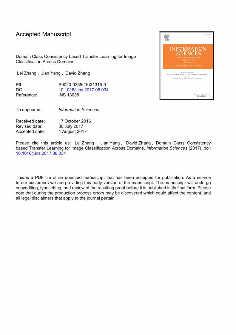
shown in Fig. 1, which explicitly shows the domain shifts/bias.
In order to deal with such domain distribution mismatch issues, transfer learning and domain adaptation
based methods have been emerged [4, 13, 16, 20, 32, 33, 40, 41, 42], which can be generally divided into two
categories: classifier-based and feature-based. Specifically, the classifier based methods advocate learning a
transfer classifier on the source data, by leveraging a few labeled data from the target domain simultaneously
[1, 4, 5, 6, 40, 42]. The “borrowed” target data implies the role of regularization, which can trade-off the
decision boundary, such that the learned decision function (e.g. SVM) is posed the transfer capability and can
be used for classification of domains with bias. The idea of classifier based techniques is straightforward and
easy to understand, however, during the decision boundary determination, a number of labeled data are
ACCEPTED MANUSCRIPT
ACCEPTED MANUSCRIP
T
3
necessary, which may increase the cost of data labeling. Essentially, the classifier based methods attempt to
learn a generalized decision function without mining the intrinsic visual drifting mechanism, thus they cannot
solve the distribution mismatch fundamentally.
Fig. 1. Examples of object images from 4 sources: Amazon (1st row), DSLR (2nd row), Webcam (3rd row) and Caltech (4th row).
Further, the feature based representation and transformation methods [9, 12, 13, 43, 44] aim at aligning the
domain shift by adapting features from the source domain to target domain without training classifiers.
Although these methods have been proven to be effective for domain adaptation, two issues still exist. First,
for representation based adaptation, the noise and outliers from source data may also be transferred to target
data due to overfitting of naïve transformation, which leads to significantly distorted and corrupted data
structure. Second, the learned subspace is suboptimal, due to the fact that the subspace and the representation
(e.g. global low-rank, local sparse coding etc.) are learned independently, which limits the transfer ability.
Third, nonlinear transfer often happens in real application, and cannot be effectively interpreted by using
linear reconstruction. Therefore, subspace learning and kernel learning that help most to representation
transfer and nonlinear transfer should be conducted and integrated simultaneously.
Additionally, Long, et al. [24, 25] proposed class-wise adaptation regularization method (ARTL) which
learns an adaptive classifier by jointly optimizing the structural risk and distribution matching between both
marginal and conditional distribution for transfer learning. Considering the labeling cost of target domain,
unsupervised domain adaptation methods have been proposed [11, 26]. By leveraging the strong learning
capability of deep learning, with the convolution neural network (CNN) and maximum mean discrepancy
(MMD) criteria, deep transfer learning methods such as residual transfer network (RTN) [27], deep
adaptation network (DAN) [28, 29], and joint CNN model [37, 38] have also been proposed. Deep transfer
learning depends on pre-trained knowledge network on a larger dataset (e.g. ImageNet), so that the transfer
ACCEPTED MANUSCRIPT
ACCEPTED MANUSCRIP
T
4
performance is greatly improved. In this paper, the proposed method is essentially a shallow transfer learning
model, therefore, for comparing with deep transfer models, the CNN based deep features (e.g. DeCAF) are
exploited in this paper.
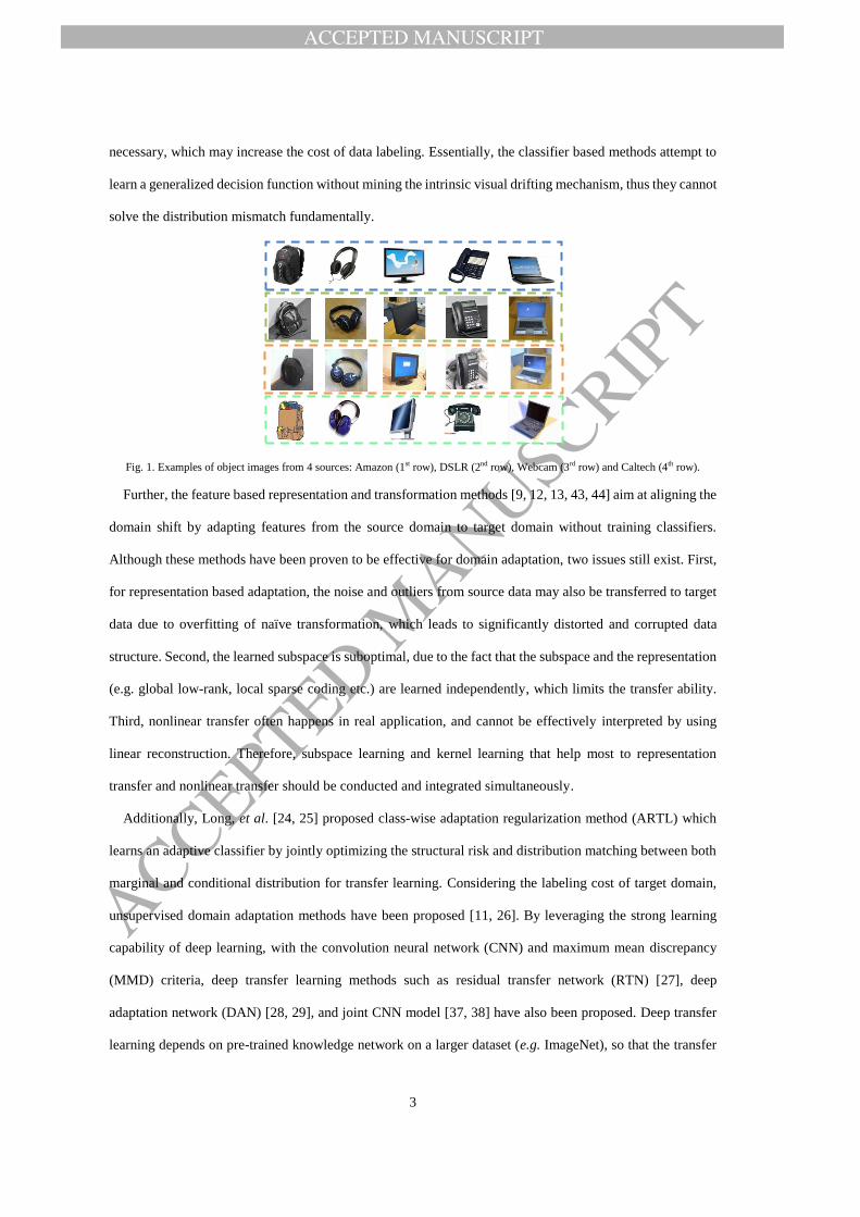
Fig. 2. Schematic diagram of the proposed DKTL method. The data points of 3 classes (i.e. c1, c2, and c3) with different marker are
included in source domain and target domain. The space distribution disparity and potential outliers per class are clearly shown. Our task
is to learn a discriminative subspace projection P in RKHS, such that the data points from both domains can lie in a shared subspace
where the sparse reconstruction (representation) is implemented for learning such a correspondence Z robust to outliers.
As described in Fig.2, in this paper, we propose a novel model which targets at learning a discriminative
subspace P by using a newly proposed domain-class-consistency metric, a reproduced kernel Hilbert space,
and a l2,1-norm constrained representation. This work is an extension of the IJCNN conference paper [45], by
adding more detailed algorithmic deduction and discussion throughout the paper, conducting new
experiments on benchmark datasets, introducing parameter sensitive analysis, empirical comparison of
computational time, and comparing with more deep transfer learning methods. The proposed method has
three merits:
(1) It can learn a discriminative subspace for each domain and guarantee the maximum separability of
different classes (i.e. c1, c2, c3.) within the same domain. In the model, we formulate to maximize the
inter-class distance within the same domain, such that the inter-class difference within a domain can cover
the between-domain discrepancy. In this way, the inter-class difference can be enhanced and the impact of
distribution mismatch is thus reduced, such that the proposed method is not sensitive to domain bias. This is
Discriminative subspace
c3 c3
c2 c2 c1 c1
Outlier removal
Outlier
O
Source domain Target domain
P
P
Z
RKHS
RKHS
ACCEPTED MANUSCRIPT
ACCEPTED MANUSCRIP
T
5
motivated by the fact that in face recognition, the difference between two images of the same person captured
under different illumination condition may be larger than that of two persons captured under the same
condition.
(2) By imposing l2,1-norm constraint on the transfer representation coefficient Z between source and target
data points, only a few valuable source data points are utilized, such that the outliers in the source domain can
be well removed without incorrectly transferring to the target domain. Therefore, the proposed method is not
sensitive to noises or implicit outliers during transferring. Additionally, with the l2,1-norm constraint on Z, the
closed-form solution can be obtained with a higher computational efficiency than l1-norm sparse constraint or
low-rank constraint.
(3) Due to the fact that nonlinear domain shift may often be encountered in complex vision applications,
the kernel learning idea using an implicit nonlinear mapping function for approximated linear separability in
the reproduced kernel Hilbert space (RKHS) is naturally motivated. With the above description,
discriminative subspace learning, representation learning and kernel learning are formulated in the proposed
method. For convenience, we call our method discriminative kernel transfer learning (DKTL).
The rest of this paper is organized as follows. Section 2 summarizes the related work in transfer learning
and domain adaptation. The proposed model and optimization algorithms are presented in Section 3. The
experiments on a number of datasets for transfer learning tasks and discussions are conducted in Section 4.
The parameter sensitivity and computational time analysis are provided in Section 5. Finally, a concluding
remark of the present work is given.
2. Related Work
In recent years, a number of transfer learning and domain adaptation methods have been proposed, which
are summarized as two categories: classifier adaptation based methods and feature adaptation based methods.
For the former, Yang et al. [40] proposed an adaptive support vector machine (ASVM), which aims at
learning the perturbation term for adapting the source classifier to the target classifier. Collobert et al. [1]
proposed a transductive SVM (T-SVM), which utilized the labeled and unlabeled samples simultaneously.
Duan et al. [5] proposed a domain adaptation machine (DAM) method which integrates SVM for classifier
adaptation. With the SVM based classifier adaptation idea, they also proposed an adaptive multiple kernel

ACCEPTED MANUSCRIPT
ACCEPTED MANUSCRIP
T
6
learning method (AMKL) [6] and a domain transfer MKL (DTMKL or DTSVM) [4] methods, by integrating
multiple kernels for improving the robustness and classification accuracy. Zhang et al. proposed a domain
adaptation ELM method for classifier adaptation [42], and also proposed a robust extreme domain adaptation
(EDA) [46] method by using Laplacian graph regularization for local structure preservation and achieve
state-of-the-art results. Zheng et al. [47] proposed a hetero-manifold regularization method (HMR) for
cross-modal hashing and achieves good results on cross-modal tasks. Shekhar et al. [36] proposed a domain
adaptive dictionary learning method (SDDL) for representation classifier adaptation. Zhu and Shao [48] also
proposed a cross-domain dictionary learning method (WSCDDL) for weakly-supervised transfer learning
based on representation classifier adaptation. Based on the cross-domain dictionary learning, Zhu et al. [49]
proposed a boosted cross-domain categorization (BCDC) method and a more robust cross-domain classifier
was contributed.
For the latter, Gopalan et al. [13] proposed a SGF method for unsupervised domain adaptation via low
dimensional subspace transfer. The idea behind SGF is that it samples a group of subspaces along the
geodesic between source and target data, and project the source data into the subspaces for discriminative
classifier learning. Gong et al. [12] proposed an unsupervised domain adaptation method (GFK) for visual
domain adaptation, in which geodesic flow kernel is used to model the domain shift by integrating an infinite
number of subspaces, where the geometric and statistical properties are characterized. Zhang et al. [43]
proposed a latent sparse domain transfer (LSDT) method by using sparse subspace reconstruction for visual
adaptation. Fernando et al. [9] proposed principal component subspace alignment (SA) for subspace transfer.
More recently, low rank representation (LRR) based domain adaptation is proposed. Two representative
work can be referred as [18, 34], in which LRR based method are proposed for aligning the domain shifts. As
referred by Liu et al. [22, 23], LRR can get the block diagonal solution and performs perfectly for subspace
segmentation when the subspaces are independent and the data sampling is sufficient. However, when
handling disjoint subspace problems and insufficient data, LRR will not work well. Therefore, LRR based
domain adaptation capability will be restricted because of such strong independent subspace assumption. An
excellent survey on transfer learning for visual categorization by Shao, et al. can be referred to as [35], which
has well explored the existing methods.
As indicated by the sparse subspace clustering (SSC) [7, 8], which were proposed for clustering data points

ACCEPTED MANUSCRIPT
ACCEPTED MANUSCRIP
T
7
that lie in a union of multiple low-dimensional subspaces or near the intersections of subspaces, the
reconstruction errorF
XZX is minimized by imposing sparsity constraint on Z. Therefore, in transfer
learning tasks, the cross-domain reconstruction error F
ZXX ST is expected to be minimized for adapting
source data to target data lying in different subspaces. However, this reconstruction error minimization
problem only guarantees the data consistency, but missing the domain transfer property. That is, there is no
knowledge adaptation based on such naïve least square. Therefore, we propose to achieve the minimization
in some latent subspace P, i.e. F
ZPXPX ST . Also, to guarantee the inter-class separability in the subspace,
discriminative subspace with domain-class-consistency (i.e. DCC) can be simultaneously learned.
3. Proposed Discriminative Kernel Transfer Learning
3.1. Notations
In this paper, the source and target domain are defined by subscript “S” and “T”. The training set of source
and target domain is defined as SNDS
X and TND
T
X , where D denotes the dimension of data, NS
and NT denote the number of samples of source and target domain, respectively. Let )( DddD P
represent the discriminative basis transformation that maps the original data space of the source and target
data into a d dimensional subspace. The reconstruction coefficient matrix is denoted as Z, and I denotes the
identity matrix. ‖ ‖ , ‖ ‖ and‖ ‖ denote lp-norm, lq,p-norm and Frobenius norm, respectively. The
superscript T denotes the transpose operator, and Tr(·) denotes the trace operator of a matrix.
3.2. Problem Formulation
As illustrated in Fig. 2, we tend to learn a representation matrix Z for reconstructing the target data XT by
using the source data XS in their discriminative subspace projected by a group of basis, i.e. P. Therefore, the
general framework of the proposed DKTL can be formulated as
0,,..
,,,min
T
,
IPP
ZPZPXXZP
ts
RE TS
(1)
where ( ) represents the domain-inconsistency term (i.e. cross domain representation or reconstruction
error), ( ) denotes the class-inconsistency term (i.e. discriminative regularizer) among multiple domains,

ACCEPTED MANUSCRIPT
ACCEPTED MANUSCRIP
T
8
( ) represents the model regularization term of the representation coefficients with robust outlier removal, λ
and τ represent the positive regularization parameters. The constraint condition guarantees the
normalized orthogonal subspace of P.
From the optimization problem (1), it is obvious that by jointly minimizing the domain-inconsistency and
class-inconsistency, i.e. DCIC, the domain-class-consistency (DCC) can be strengthened such that the
proposed DKTL not only realizes the domain transfer (i.e. domain consistency), but also enhances the class
separability (i.e. class consistency). Therefore, the proposed model is more robust for classification-oriented
transfer learning tasks. Note that maximization of the domain-class-consistency (DCC) is equivalent to
minimize the domain-class-inconsistency (DCIC), but for easier formulation, a DCIC minimization problem
is solved in this paper.
Suppose that P can be represented by a linear combination of the transformed training samples ( )
[ ( ) ( )], which can be written as
ΦXP (2)
where dNΦ denotes the linear combination coefficients, is some implicit linear/nonlinear mapping
function imposed on the raw data, and N=NS+NT.
Specifically, by substituting Eq.(2) and the mapping function into the first term of Eq.(1), then the
reconstruction error expression ( ) can be formulated as follows
2
F
TTTT
2
F
TT,,,
ZXXΦXXΦ
ZXPXPZPXX
ST
STTSE
(3)
where denotes the cross domain representation coefficient matrix. Obviously, the smaller the
representation error ( ) is, the better the domain consistency is. Therefore, by minimizing the
reconstruction error in the latent subspace, the domain consistency can be enhanced.
The second term ( ) in Eq.(1) pursuits a discriminative subspace where the domain-class-inconsistency
(DCIC) is minimized. As the name suggests, the DCIC includes two parts: domain inconsistency (minimized)
and class inconsistency (maximized). Therefore, the DCIC term can be formulated as

ACCEPTED MANUSCRIPT
ACCEPTED MANUSCRIP
T
9
TSt
C
kckc
kt
ct
C
c
cT
cS
TSt
C
kckc
kt
ct
C
c
cT
cS
, ,1,
2
2
TTTT
1
2
2
TTTT
, ,1,
2
2
TT
1
2
2
TT
μXΦμXΦμXΦμXΦ
μPμPμPμPP
(4)
where
cSN
i
ciSc
S
cS
N 1,
1Xμ and
cTN
i
ciTc
T
cT
N 1,
1Xμ represent the centroid of class c of source and
target training data after ( ) mapping, respectively. The first term in Eq.(4) denotes the between-domain
intra-class inconsistency (i.e. the same class in different domain) that expects to be minimized and the second
term in Eq.(4) denotes the within-domain inter-class consistency (i.e. different class in the same domain) that
expects to be maximized. Note that a very few labeled target data should be used during the computation of
Eq.(4) in the proposed method, that is, DKTL is not unsupervised. However, it is not difficult to obtain an
unsupervised variant by only considering the labeled source data. For example, for the target domain data, the
centroid of the unlabeled target data can be computed for measuring inter-domain discrepancy. By
minimizing the difference between the intra-class inconsistency and the inter-class consistency, the
discriminative subspace can be well achieved. Consequently, the generalized domain-class-consistency can
be well shown, and the discriminative learning can effectively improve the classification-oriented domain
transfer performance.
The third term ( ) in Eq.(1) is a robust sparse constraint on the transfer coefficients Z for regularization.
Generally, it can be formulated as follows
pq
R,
ZZ (5)
where ‖ ‖ represents lq,p-norm. Given a matrix nmQ , then there is
pm
i
qpn
j
q
jipqQ
1
1 1,,
Q (6)
As can be seen from Eq.(6), a common Frobenius norm is achieved when p=q=2. Intrinsically, different
approaches may be induced by selecting different p and q-values. Generally, for sparsity pursuit, q≥2 and
0≤p≤2 may be required. If p=0, the induced l0-norm sub-problem is not convex and therefore p=1 is used in
this paper for sparse approximation. Since q is used to measure the row vector norm, q=2 is set based on the

ACCEPTED MANUSCRIPT
ACCEPTED MANUSCRIP
T
10
consideration that larger q does not improve the results [17]. Therefore, the Eq.(5) can be formulated by
l2,1-norm as ( ) ‖ ‖ for better sparsity and robustness to outliers. The property of l2,1-norm guarantees
that the outliers in source data can be automatically avoided during representation transfer. In this way, the
implicit outliers in source domain may not be transferred to target domain via l2,1-norm minimization, such
that the generalization is achieved.
Finally, by substituting Eqs.(3), (4) and (5) into Eq.(1), the proposed DKTL model can be formulated as
follows
0,,..
min
TT
1,2, ,1,
2
2
TTTT
1
2
2
TTTT2
F
TTTT
,
IΦXXΦ
ZμXΦμXΦ
μXΦμXΦZXXΦXXΦZΦ
ts
TSt
C
kckc
kt
ct
C
c
cT
cSST
(7)
According to the Mercer kernel theorem and inner product, we define the following kernel matrices,
XXXXK ,T
TTT XXXXK ,T
SSS XXXXK ,T
cS
cS
cS μXμXK ,
T,
cT
cT
cT μXμXK ,
T,
Then the proposed DKTL model (7) can be reformulated as
0,,,,1,..
1
2
1min
T
1,2, ,1,
2
2,
T,
T
1
2
2,
T,
T2
F
TT
,
TSTS
TSt
C
kckc
kt
ctt
C
c
cT
cSST
ts
CC
C
IKΦΦ
ZKΦKΦ
KΦKΦZKΦKΦZΦ
(8)
where the coefficient αS and αT represent the weights of source and target domain, which are used to weight
the within-domain inter-class difference and improve class-consistency (e.g. if source domain has larger

ACCEPTED MANUSCRIPT
ACCEPTED MANUSCRIP
T
11
inter-class discrepancy than target domain, and therefore αS should be slightly larger than αT). λ and τ
represent the regularization parameters for DCIC term and reconstruction matrix Z, respectively, which are
used to trade-off the domain transfer performance. , , and denote the kernel Gram matrix of the
combined data, source data and target data, respectively. and
denote the kernel mean vectors with
respect to class c of source data and target data, respectively. ( ) represents the kernel function. From
Equation (8), it is clear that the proposed transfer learning model is transformed into a kernel reconstruction
framework in RKHS space. Generally, the effect of kernel is to reproduce a rich embedding space where the
distribution matching (i.e. domain transfer) can be easily implemented. Although different kernel functions
such as polynomial kernel, perceptron kernel (i.e. sigmoid), etc. can be used, Gaussian kernel can reproduce
richer embedding space for transferring.
Therefore, in this paper, the Gaussian kernel function is used, and it can be represented with kernel
parameter σ by
22
22exp, yxyx (9)
From Eq.(8), it is clear that this is a non-convex optimization problem with respect to two variables Φ and
Z. However, it becomes a convex problem with respect to one variable by fixing the other one. Therefore, a
common variable alternating optimization algorithm is proposed for near-optimal solutions. The specific
solving process is presented as follows.
3.3. Optimization
The optimization of DKTL model (8) is presented in this section. From Eq.(8), there are two variables Φ
and Z in the model. When fix one of them, the model is convex with respect to the other one. Therefore, a
variable alternating optimization algorithm is proposed for solving the minimization problem.
Update Φ:
By fixing the variable Z, the problem shown in Eq.(8) with respect to Φ then becomes
ACCEPTED MANUSCRIPT
ACCEPTED MANUSCRIP
T
12
0,,,1,..
1
21min
T
, ,1,
2
2,
T,
T
1
2
2,
T,
T2
F
TT
TSTS
TSt
C
kckc
kt
ctt
C
c
cT
cSST
ts
CCC
IKΦΦ
KΦKΦKΦKΦZKΦKΦΦ
(10)
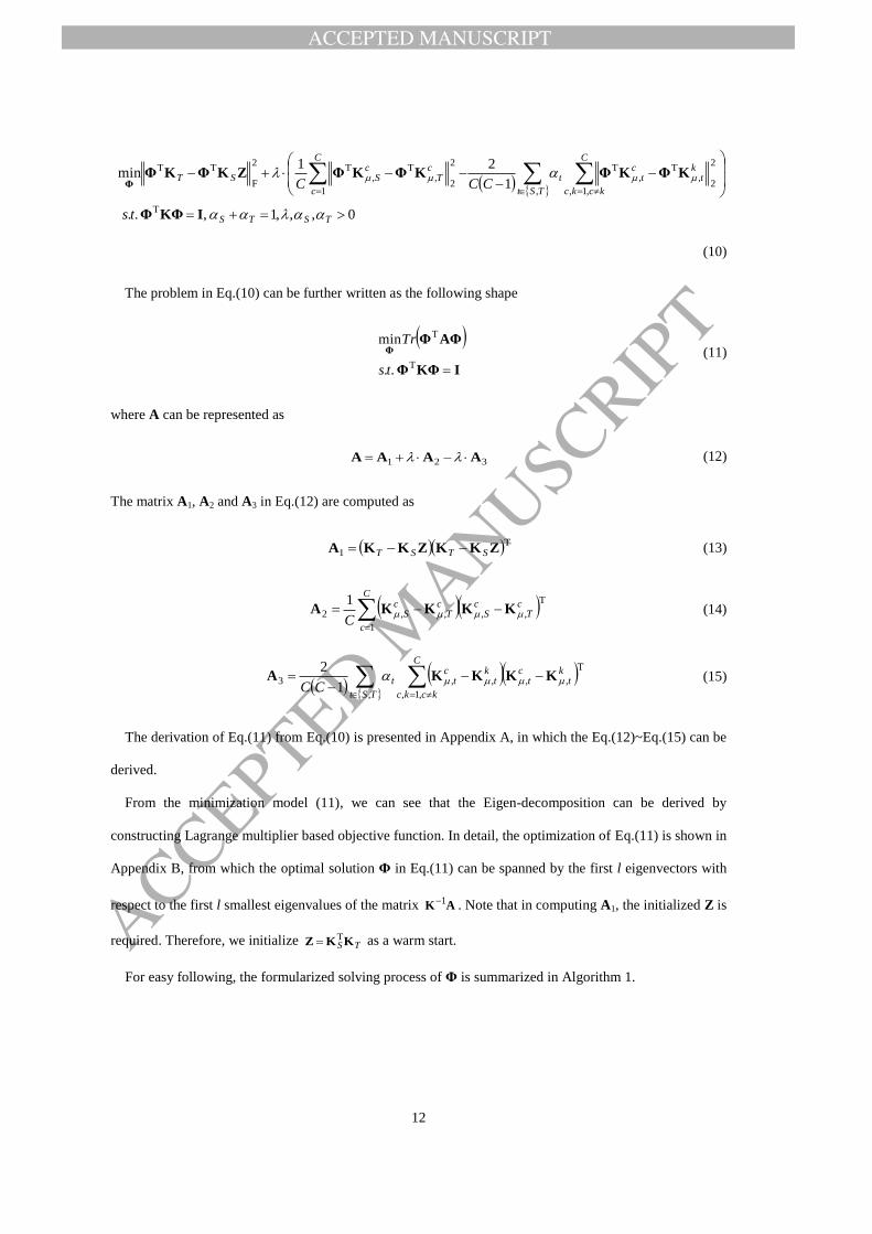
The problem in Eq.(10) can be further written as the following shape
IKΦΦ
AΦΦΦ
T
T
..
min
ts
Tr (11)
where A can be represented as
321 AAAA (12)
The matrix A1, A2 and A3 in Eq.(12) are computed as
T1 ZKKZKKA STST (13)
C
c
cT
cS
cT
cS
C1
T
,,,,2
1 KKKKA (14)
TSt
C
kckc
kt
ct
kt
ctt
CC, ,1,
T
,,,,31
2 KKKKA (15)
The derivation of Eq.(11) from Eq.(10) is presented in Appendix A, in which the Eq.(12)~Eq.(15) can be
derived.
From the minimization model (11), we can see that the Eigen-decomposition can be derived by
constructing Lagrange multiplier based objective function. In detail, the optimization of Eq.(11) is shown in
Appendix B, from which the optimal solution Φ in Eq.(11) can be spanned by the first l eigenvectors with
respect to the first l smallest eigenvalues of the matrix AK1 . Note that in computing A1, the initialized Z is
required. Therefore, we initialize TS KKZT as a warm start.
For easy following, the formularized solving process of Φ is summarized in Algorithm 1.

ACCEPTED MANUSCRIPT
ACCEPTED MANUSCRIP
T
13
Algorithm 1. Solving Φ
Input: SK , TK , cS,K , c
T,K , λ, d;
Procedure:
1. Initialize TS KKZT ;
2. Compute A1, A2 and A3 using Eqs.(13), (14), (15),
respectively;
3. Compute A using Eq.(12);
4. Perform Eigen-value decomposition of T1UUAK ;
5. Get :,UΦ , where is the index of the d smallest
Eigen-values;
Output: Φ
Update Z:
By fixing Φ, the problem in Eq.(8) is transformed into the following problem
1,2
2
F
TTmin ZZKΦKΦZ
ST (16)
The second term in Eq.(16) can be written as [31].
ΘZZZT
1,2Tr (17)
where SS NN Θ is a diagonal matrix, whose the i-th diagonal element is calculated as
22
1
iiiΘ
Z (18)
where iZ represents the i-th row of matrix Z.
By substituting Eq.(17) into Eq.(16), we have
ΘZZZKΦKΦZ
T2
F
TTmin TrST (19)
As can be seen from model (19), it is differentiable with respect to Z. Let its derivative be 0, we have
TSSS KΦΦKZΘKΦΦKTTTT (20)

ACCEPTED MANUSCRIPT
ACCEPTED MANUSCRIP
T
14
Then, the closed-form solution of Z can be expressed as
TSSS KΦΦKΘKΦΦKZTT-1TT (21)
For easy following, the optimization of Z is summarized in Algorithm 2.
Although the closed-form solution of Z can be achieved, in computing Θ , the initialized Z is required.
Therefore, for achieving the optimal solutions Z* and via variable alternating optimization method,
several iterations can guarantee the convergence.
Algorithm 2. Solving Z
Input: KS, KT, Φ, τ;
Procedure:
1. Initialize TS KKZT ;
2. Compute Θ using Eq.(18);
3. Compute Z using Eq.(21);
Output: Z;
By recalling the optimization of in Algorithm 1 and the optimization of Z in Algorithm 2, the whole
optimization process of the proposed DKTL model shown in Eq.(8) can be summarized in Algorithm 3.
Algorithm 3. Proposed DKTL
Input: SK , TK , cS,K , c
T,K , λ, τ, d, Tmax;
1. Initialize TS KKZT and t=1;
2. While not converged (t<Tmax) do
3. Update Φ by calling Algorithm 1;
4. Update Z by calling Algorithm 2;
5. Compute the objective function value using Eq.(8)
6. t=t+1;
7. Until Convergence;
Output: Z* and Φ
*;

ACCEPTED MANUSCRIPT
ACCEPTED MANUSCRIP
T
15
3.4. Computational Complexity
The Algorithm 3 of DKTL includes two steps: update Φ (algorithm 1) and update Z (algorithm 2). For
algorithm 1, the Eigen-decomposition is involved with complexity of O(N3); for Algorithm 2, the matrix
inverse and multiplication are involved with complexity of O(N3). Therefore, the total complexity of DKTL
with T iterations is O(TN3). It is worth noting that the closed-form solution of Z can be obtained with
l2,1-norm, such that the computation of Z is largely reduced by comparing with that of l1-norm (e.g. ADMM)
or low-rank (e.g. ALM) constraints on Z. Further, the computational time comparison on different tasks is
given in Section 5.2.
3.5. Classification
In this paper, we attempt to reduce the domain bias by learning a target data reconstruction model in
some latent subspace. The proposed DKTL is independent of classification, and the classification is
implemented after solving the optimal Z and .
The projected source data in RKHS is represented as and the reconstructed target data can
be represented as . Then, existing classification methods (e.g. nearest neighbor,
regularized least square, support vector machine) can be used for training a classifier based on the source data
( ), and the recognition/test is done on the target data (
). Note that and denote the labels
with respect to source data and target data, respectively.
4. Experiments
In this section, the experiments on several benchmark datasets, including 3DA object data, 4DA object
data, COIL-20 object data, Multi-PIE face data, USPS data, SEMEION data, and MINIST handwritten digits
data, have been conducted for evaluating the proposed DKTL method. For classification, the regularized
least square classifier and support vector machine can be used.
4.1. Cross-domain Object Recognition
In the experiments of object recognition, we test our method in three domain adaptation benchmark
datasets: 3DA office dataset, 4DA office dataset, and COIL-20 object dataset.
3DA data: Amazon, DSLR and Webcam [33].

ACCEPTED MANUSCRIPT
ACCEPTED MANUSCRIP
T
16
Table 1
Classification Accuracy (%) over 31 Object Categories of Single Source Domain Adaptation in 3DA Data
Tasks ASVM [40] GFK [12] SGF [13] RDALR [18] SA [9] LTSL [34] DKTL
Amazon → Webcam 42.2±0.9 46.4±0.5 45.1±0.6 50.7±0.8 48.4±0.6 53.5±0.4 53.0±0.8
DSLR → Webcam 33.0±0.8 61.3±0.4 61.4±0.4 36.9±1.9 61.8±0.9 62.4±0.3 65.7±0.4
Webcam → DSLR 26.0±0.7 66.3±0.4 63.4±0.5 32.9±1.2 63.4±0.5 63.9±0.3 73.3±0.5
Table 2
Classification Accuracy (%) over 31 Object Categories of Multiple Source Domains Adaptation in 3DA data
Tasks ASVM [40] GFK [12] SGF [13] RDALR [18] SA [9] LTSL [34] DKTL
Amazon+DSLR→Webcam 30.4±0.6 34.3±0.6 31.0±1.6 36.9±1.1 54.4±0.9 55.3±0.3 60.0±0.5
Amazon+Webcam→DSLR 25.3±1.1 52.0±0.8 25.0±0.4 31.2±1.3 37.5±1.0 57.7±0.4 63.7±0.7
DSLR+Webcam→Amazon 17.3±0.9 21.7±0.5 15.0±0.4 20.9±0.9 16.5±0.4 20.0±0.2 22.0±0.4
It’s clear that 3DA dataset includes 4106 samples from three domains, where each domain contains 31
object classes, such as back-pack, keyboard, earphone, etc. By following [33], the 800-bin SURF features are
used. 5 random splits of the training data in the source and target domain are implemented and the mean
accuracies over 31 categories for a single source domain and multiple source domains adaptation are reported
in Table 1 and Table 2, respectively. We compare with six methods, including ASVM [40], GFK [12], SGF
[13], SA [9], RDALR [18] and LTSL [34]. From the results, we can observe that LSDT with nonlinear kernel
function performs much better results than other methods for single source domain adaptation. For
multi-source domain adaptation, DKTL outperforms other methods. Additionally, LTSL outperforms
RDALR method to a large extent. Therefore, LTSL is compared in the following experiments.
4DA data: Amazon, DSLR, Webcam and Caltech [12].
In 4DA dataset, four domains with 2433 samples are included, where each domain contains 10 common
object classes selected from 3DA dataset and an extra Caltech 256 dataset. In experiments, the deep
convolutional activation feature (DeCAF) of 4DA data is exploited [3]. The CNN with 5 convolutional layers
and 3 fully-connected layers is trained on ImageNet-1000 [19]. For deep feature representation of 4DA, the

ACCEPTED MANUSCRIPT
ACCEPTED MANUSCRIP
T
17
outputs of the 7th
fully-connected layer are used as deep features of the 4DA dataset.
Table 3
Classification Accuracy (%) of Different Domain Adaptation based on CNN Feature in 4DA Setting
Method A→D C→D A→C W→C D→C D→A W→A C→A C→W A→W
NaïveComb 94.1±0.8 92.8±0.7 83.4±0.4 81.2±0.4 82.7±0.4 90.9±0.3 90.6±0.2 90.3±0.2 90.6±0.8 91.1±0.8
SGF [13] 92.0±1.3 92.4±1.1 77.4±0.7 76.8±0.7 78.2±0.7 88.0±0.5 86.8±0.7 89.3±0.4 87.8±0.8 88.1±0.8
GFK [12] 94.3±0.7 91.9±0.8 79.1±0.7 76.1±0.7 77.5±0.8 90.1±0.4 85.6±0.5 88.4±0.4 86.4±0.7 88.6±0.8
SA [9] 92.8±1.0 92.1±0.9 83.3±0.2 81.0±0.6 82.9±0.7 90.7±0.5 90.9±0.4 89.9±0.5 89.0±1.1 87.8±1.4
LTSL [34] 94.5±0.5 93.5±0.8 85.4±0.1 82.6±0.3 84.8±0.2 91.9±0.2 91.0±0.2 90.9±0.1 90.8±0.7 91.5±0.5
DKTL 96.6±0.5 94.3±0.6 86.7±0.3 84.0±0.3 86.1±0.4 92.5±0.3 91.9±0.3 92.4±0.1 92.0±0.9 93.0±0.8
Table 4
Comparisons with deep transfer learning methods on 4DA dataset
Method A→D C→D A→C W→C D→C D→A W→A C→A C→W A→W Average
AlexNet [19] 88.3 87.3 77.9 77.9 81.0 89.0 83.1 91.3 83.2 83.1 84.2
DDC [38] 89.0 88.8 85.0 78.0 81.1 89.5 84.9 91.9 85.4 86.1 86.0
DAN [28] 92.4 90.5 85.1 84.3 82.4 92.0 92.1 92.0 90.6 93.8 89.5
RTN [27] 94.6 92.9 88.5 88.4 84.3 95.5 93.1 94.4 96.6 97.0 92.5
DKTL 96.6 94.3 86.7 84.0 86.1 92.5 91.9 92.4 92.0 93.0 91.0
We strictly follow the experimental setting by Gong et al.[12], 20 random splits of the training data are
used, and the mean classification accuracies on CNN deep features are reported in Table 3. By comparing to
state-of-the-art methods, from Table 3, we can clearly observe that DKTL performs much better than LTSL
and also outperforms other methods. Further, we have also compared with several deep transfer learning
methods, such as AlexNet [19], deep domain confusion (DDC) [38], deep adaptation network (DAN) [28],
and residual transfer network (RTN) [27] on the 4DA dataset. The comparisons are shown in Table 4.
Notably, for our method, the off-the-shelf CNN based DeCAF feature is used for fair comparison. Due to that
the repetitive running experiments of these deep transfer models are not easy, for better subjectivity, the
results in Table 4 of deep transfer learning methods are copied from the RTN paper [27]. From Table 4, we

ACCEPTED MANUSCRIPT
ACCEPTED MANUSCRIP
T
18
can see that although the RTN shows better performance than DKTL, our method still shows competitive
performance among deep transfer models. Specifically, the average result of DKTL is 91%, which is 1.5%
lower than RTN, but 1.5% higher than DAN, and 6.8% higher than AlexNet. Additionally, the visualization
of the representation based transfer coefficients Z can be observed in Fig. 3.
(a) Z on 4DA data (b) Z on 3DA data
Fig. 3. Visualization of the solved representation coefficients Z
Fig. 4. Several objects from COIL-20 data (e.g. COIL 1, 2, 3, and 4)
COIL-20 data: Columbia Object Image Library [30].
The domain adaptation experiment on COIL-20 dataset was first announced by Long et al. [25]. The
COIL-20 dataset contains 1440 gray scale images of 20 objects (72 images with different poses per object).
The objects have a wide variety of complex geometric and reflectance characteristics, and can effectively
validate the cross domain learning models. Each image has 128×128 pixels with 256 gray levels per pixel.
For experiments, the size of each image is adjusted as 32×32 [39]. Some example images of this dataset are
shown in Fig. 4.
5 10 15 20 25 30
20
40
60
80
100
120
140
160
180
200-0.4
-0.2
0
0.2
0.4
0.6
0.8
10 20 30 40 50 60 70 80 90
50
100
150
200
-0.1
0
0.1
0.2
0.3
0.4
0.5
ACCEPTED MANUSCRIPT
ACCEPTED MANUSCRIP
T
19
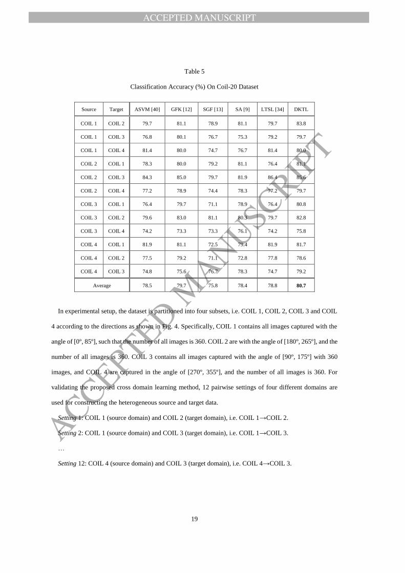
Table 5
Classification Accuracy (%) On Coil-20 Dataset
Source Target ASVM [40] GFK [12] SGF [13] SA [9] LTSL [34] DKTL
COIL 1 COIL 2 79.7 81.1 78.9 81.1 79.7 83.8
COIL 1 COIL 3 76.8 80.1 76.7 75.3 79.2 79.7
COIL 1 COIL 4 81.4 80.0 74.7 76.7 81.4 80.0
COIL 2 COIL 1 78.3 80.0 79.2 81.1 76.4 81.1
COIL 2 COIL 3 84.3 85.0 79.7 81.9 86.4 85.6
COIL 2 COIL 4 77.2 78.9 74.4 78.3 77.2 79.7
COIL 3 COIL 1 76.4 79.7 71.1 78.9 76.4 80.8
COIL 3 COIL 2 79.6 83.0 81.1 80.3 79.7 82.8
COIL 3 COIL 4 74.2 73.3 73.3 76.1 74.2 75.8
COIL 4 COIL 1 81.9 81.1 72.5 79.4 81.9 81.7
COIL 4 COIL 2 77.5 79.2 71.1 72.8 77.8 78.6
COIL 4 COIL 3 74.8 75.6 76.7 78.3 74.7 79.2
Average 78.5 79.7 75.8 78.4 78.8 80.7
In experimental setup, the dataset is partitioned into four subsets, i.e. COIL 1, COIL 2, COIL 3 and COIL
4 according to the directions as shown in Fig. 4. Specifically, COIL 1 contains all images captured with the
angle of [0º, 85º], such that the number of all images is 360. COIL 2 are with the angle of [180º, 265º], and the
number of all images is 360. COIL 3 contains all images captured with the angle of [90º, 175º] with 360
images, and COIL 4 are captured in the angle of [270º, 355º], and the number of all images is 360. For
validating the proposed cross domain learning method, 12 pairwise settings of four different domains are
used for constructing the heterogeneous source and target data.
Setting 1: COIL 1 (source domain) and COIL 2 (target domain), i.e. COIL 1→COIL 2.
Setting 2: COIL 1 (source domain) and COIL 3 (target domain), i.e. COIL 1→COIL 3.
…
Setting 12: COIL 4 (source domain) and COIL 3 (target domain), i.e. COIL 4→COIL 3.

ACCEPTED MANUSCRIPT
ACCEPTED MANUSCRIP
T
20
The experimental results for 12 settings are reported in Table 5, from which we can observe that the
proposed DKTL method achieves the best performance with an average recognition accuracy of 80.7%.
Fig. 5. CMU Multi-PIE data. Session 1 (the 1st row with neutral expression) and Session 2 (the 2nd row with smile
expression)
4.2. Cross-poses Face Recognition
The CMU Multi-PIE face dataset [15] is a comprehensive face dataset of 337 subjects, in which the images
are captured across 15 poses, 20 illuminations, 6 expressions and 4 different sessions. For our purpose, we
select the first 60 subjects from session 1 and session 2 in experiments. Session 1 contains 7 images per
subject with 7 poses under neutral expression, while session 2 was prepared with the same poses as session 1
under smile expression. Similar domain adaptation experiment on PIE has been first conducted by Long et al.
[25]. In this paper, four cross-domain recognition tasks are as follows.
Session 1 (cross-poses): one frontal face and an extreme pose with 60º angle for each subject are used as
source and target data, respectively. The remaining faces are used as probe faces.
Session 2 (cross-poses): the same configuration as session 1 is conducted on session 2.
Session 1+2 (cross-poses): Two frontal faces and two faces with extreme 60º pose from both sessions
are selected as source and target data. The remaining faces with poses are used as probe faces.
Cross session: The faces in session 1 with neural expression are taken as source data, while the faces in
session 2 with smile expression are taken as target data.
Fig. 5 describes some examples of one subject which consists of two sessions (neutral vs. smile
expressions). From Fig. 5, we can observe the highly nonlinear domain mismatch between frontal faces and
posed faces, while the domain mismatch between neutral and smile faces of the same view is slightly
insignificant.
The face recognition results by using different methods are shown in Table 6. From the results, we can see
that the proposed DKTL method outperforms LTSL and others. This demonstrates that linear subspace

ACCEPTED MANUSCRIPT
ACCEPTED MANUSCRIP
T
21
transfer may not deal with such nonlinear rotation well. For cross-session task, the recognition gap is small
due to that expression change is much easier to be adapted than pose.
Table 6
Comparison with Other Methods for Face Recognition Across Poses and Expression
Cross domain tasks NaïveComb ASVM [40] SGF [13] GFK [12] SA [9] LTSL [34] DKTL
Session 1: Frontal → 60º pose 52.0 52.0 53.7 56.0 51.3 61.0 66.0
Session 2: Frontal → 60º pose 55.0 56.7 55.0 58.7 62.7 62.7 71.0
Session 1+2: Frontal → 60º pose 54.5 55.1 53.8 56.3 61.7 60.2 69.5
Cross session: Session 1 → Session 2 93.6 97.2 92.5 96.7 98.3 97.2 99.4
Fig. 6. Handwritten digits (0~9) from different sources: SEMEION (1st row), USPS (2nd row) and MINIST (3rd row)
4.3. Cross-domain Handwritten Digits Recognition
The domain adaptation experiment on handwritten digit recognition was first proposed by Long et al. [26].
In this paper, three handwritten digits datasets, MINIST [21], USPS [10] and SEMEION [10] are used for
evaluating the proposed cross domain learning method. The classification accuracies over 10 classes from
digit 0~9 are reported for different tasks. The MINIST handwritten digits dataset consists of 70,000 instances
with each image size of 28×28, the USPS dataset contains 9298 examples with each image size of 16×16, and
the SEMEION dataset contains 2593 images with each image size of 16×16.
For dimension consistency, the size of MINIST digit images is manually cropped as 16×16. The example
images of each class in MINIST, USPS and SEMEION are shown in Fig. 6, from which we can clearly
observe the significant domain mismatch across different domains.
In experiment, the cross-domain tests are explored, in which each dataset is viewed as one domain, and
therefore formulates 6 cross-domain tasks in pairwise. For the purpose of our experiments, we randomly
select 100 samples per class from a source domain for training and 10 samples per class from the target
domain for testing. In this way, 5 random splits are generated and the mean accuracies with parameter tuning

ACCEPTED MANUSCRIPT
ACCEPTED MANUSCRIP
T
22
are reported in Table 7, in which A-SVM [40], SGF [13], GFK [12] and LTSL [34] are compared with our
proposed DKTL method. From the results, we can see that the proposed method outperforms other methods
to a large extent.
Table 7
Handwritten Digits Recognition Performance Across Different Domains
Source Target NaïveComb A-SVM [40] SGF [13] GFK [12] SA [9] LTSL [34] DKTL
MINIST USPS 78.8±0.5 78.3±0.6 79.2±0.9 82.6±0.8 78.8±0.8 78.4±0.7 88.0±0.4
SEMEION USPS 83.6±0.3 76.8±0.4 77.5±0.9 82.7±0.6 82.5±0.5 83.4±0.3 85.8±0.4
MINIST SEMEION 51.9±0.8 70.5±0.7 51.6±0.7 70.5±0.8 74.4±0.6 50.6±0.4 74.9±0.4
USPS SEMEION 65.3±1.0 74.5±0.6 70.9±0.8 76.7±0.3 74.6±0.6 64.5±0.7 81.6±0.4
USPS MINIST 71.7±1.0 73.2±0.8 71.1±0.7 74.9±0.9 72.9±0.7 71.2±1.0 79.0±0.6
SEMEION MINIST 67.6±1.2 69.3±0.7 66.9±0.6 74.5±0.6 72.9±0.7 66.8±1.2 77.3±0.7
4.4. Discussion
With the above experiments on several benchmark datasets, we can observe the competitive effectiveness
of the proposed DKTL method via l2,1-norm minimization. The proposed joint domain-class-consistency
realized using a kernel sparse representation and discriminative cross-domain subspace learning shows a new
perspective and interest of transfer learning. Specifically, the following insights are observed.
1) The shadow of kernel learning, discriminative learning, subspace learning and representation learning can
be witnessed in the proposed method for transfer learning tasks. It implies that a number of statistical
machine learning methods can be well “fitted” to multi-domain tasks with appropriate transferring.
2) The fundamental problem that transfer learning aims to solve is to overcome the statistical distribution
mismatch induced cross-domain classification (e.g. source domain vs. target domain). How to quantify the
distribution mismatch metric is the basic motivation of this proposal. Robust reconstruction and calibration
between domains in some latent subspace is the main line of this paper, while a specifically designed
reconstruction error, as domain mismatch, is minimized.
3) Nonlinear transfer is a common problem in computer vision, and therefore kernel space mapping is
extremely appropriate to deal with such problems. Additionally, transferring should be conducted in a latent
ACCEPTED MANUSCRIPT
ACCEPTED MANUSCRIP
T
23
subspace, so that the testing phase can be effectively manifested based on this subspace projection.
5. Parameter Sensitivity and Computational Time Analysis
5.1. Parameter sensitivity analysis
In the proposed DKTL model, there are two hyper-parameters λ and τ. Additionally, there are also several
internal model parameters such as the dimensionality d, the kernel parameter σ, and the constrained
coefficient αS. For more insight of their impact on the model, we have provided parameter sensitivity analysis
in this section. Specifically, the hyper-parameters λ and τ are tuned in the range of 10-4
~104, the kernel
parameter σ is tuned in the range of 2-4
~24, and the coefficient αS is tuned in the range of 0~1. The optimal
dimensionality d is task-specific, therefore it is empirically tuned from low to high.
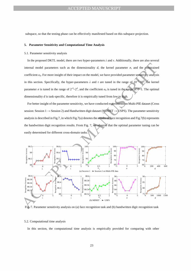
For better insight of the parameter sensitivity, we have conducted experiments on Multi-PIE dataset (Cross
session: Session 1 → Session 2) and Handwritten digit dataset (MINIST → USPS). The parameter sensitivity
analysis is described in Fig.7, in which Fig.7(a) denotes the results of face recognition and Fig.7(b) represents
the handwritten digit recognition results. From Fig. 7, we observe that the optimal parameter tuning can be
easily determined for different cross-domain tasks.
Fig. 7. Parameter sensitivity analysis on (a) face recognition task and (b) handwritten digit recognition task
5.2. Computational time analysis
In this section, the computational time analysis is empirically provided for comparing with other
-5 0 598
98.5
99
99.5
Rec
ognit
ion A
ccura
cy
-5 0 599
99.2
99.4
99.6
Rec
ognit
ion A
ccura
cy
0 0.5 194
96
98
100
s
(a) Session 1 Session 2 on Multi-PIE data
Rec
ognit
ion A
ccura
cy
-5 0 560
70
80
90
100
Rec
ognit
ion A
ccura
cy
0 200 400 60060
70
80
90
100
d
Rec
ognit
ion A
ccura
cy
-5 0 5
88.32
88.34
88.36
88.38
88.4
Rec
ognit
ion A
ccura
cy
-5 0 588
88.2
88.4
88.6
Rec
ognit
ion A
ccura
cy
0 0.5 188.52
88.54
88.56
88.58
88.6
s
(b) MINIST USPS
Rec
ognit
ion A
ccura
cy
-5 0 582
84
86
88
90
Rec
ognit
ion A
ccura
cy
0 500 1000 150075
80
85
90
d
Rec
ognit
ion A
ccura
cy

ACCEPTED MANUSCRIPT
ACCEPTED MANUSCRIP
T
24
algorithms. Specifically, we have compared with SGF [13], GFK [12], SA [9], and LTSL [34] methods on
two tasks: face recognition and handwritten digits recognition. The computational time is shown in Table 8,
where the numbers in brackets represent the recognition accuracy of each method. From Table 8, we observe
that the proposed method is slightly slower than other methods, due to the kernel computation in DKTL.
However, the domain transfer performance of the proposed method is higher than other methods. Therefore,
with the trade-off between computation and performance, the proposed DKTL still shows more competitive
results.
Table 8
Empirical computational time (s) analysis of different methods
Source Target SGF [13] GFK [12] SA [9] LTSL [34] DKTL
PIE Session 1 PIE Session 2 10.9 (92.5%) 1.50 (96.7%) 4.18 (98.3%) 7.21 (97.2%) 7.48 (99.4%)
MINIST USPS 75.0 (79.2%) 12.2 (82.6%) 30.5 (78.8%) 62.1 (78.4%) 96.9 (88.0%)
6. Conclusion
In this paper, we propose a discriminative kernel transfer learning (DKTL) via l2,1-norm minimization. In
the model, the domain class consistency (DCC) that simultaneously interprets the domain consistency and
class consistency (double consistency) is proposed. To this end, in subspace learning, the discriminative
mechanism for strengthening the importance of between-domain intra-class consistency and within-domain
inter-class inconsistency is integrated. For reducing the domain inconsistency, we tend to learn a
representation coefficient matrix between the source data and the target data in the learned discriminative
subspace. To avoid the potential outliers in source domain transferred to the target domain after
representation, the l2,1-norm constraint is imposed, such that a few valuable source data points are selected
during representation based transfer learning. Extensive experiments on several benchmark datasets
demonstrate that the effectiveness, superiority and competitiveness of the proposed DKTL method.

ACCEPTED MANUSCRIPT
ACCEPTED MANUSCRIP
T
25
Appendix A
Deduction of Eq.(11) derivation
The Eq. (10) can be re-written as
0,,,1,..
1
2
1min
T
,1,
T
,T
,T
,T
,T
,
1
T
,T
,T
,T
,TTTTTT
TSTS
C
kckc
kt
ct
kt
ct
TSt
t
C
c
cT
cS
cT
cSSTST
ts
CCTr
CTrTr
IKΦΦ
KΦKΦKΦKΦ
KΦKΦKΦKΦZKΦKΦZKΦKΦΦ
0,,,1,..
1
2
1min
T
,1,
T
,,,,
,
T
1
T
,,,,TTT
TSTS
C
kckc
kt
ct
kt
ct
TSt
t
C
c
cT
cS
cT
cSSTST
ts
CCTr
CTrTr
IKΦΦ
ΦKKKKΦ
ΦKKKKΦΦZKKZKKΦΦ
0,,,1,..
min
T
3T
2T
1T
TSTSts
TrTrTr
IKΦΦ
ΦAΦΦAΦΦAΦΦ
0,,,1,..
min
min
T
T
321T
TSTSts
Tr
Tr
IKΦΦ
AΦΦ
ΦAAAΦ
Φ
Φ
where A, A1, A2, A3 are represented in Eqs.(12), (13), (14) and (15), respectively.
Appendix B
Optimization of model Eq.(11)
According to Eq.(11), the Lagrange multiplier function ( ) can be expressed as
IKΦΦAΦΦΦ TT, Lag (22)
where ρ>0 represents the Lagrange multiplier.
By setting the derivative of Eq.(22) with respect to Φ as 0, one can obtain
ΦAΦKKΦAΦ -1 (23)

ACCEPTED MANUSCRIPT
ACCEPTED MANUSCRIP
T
26
From Eq.(23), we can get that Φ can be solved by using the following Eigen-value decomposition
T-1UUAK (24)
Then, Φ is represented by the first l Eigen-vectors in U, with respect to the first l minimum Eigen-values of
the matrix .
Acknowledgment
The authors would like to thank the AE and anonymous reviewers for their insightful and constructive
comments. This work was supported by the Fundamental Research Funds for the Central Universities
(Project No. 106112017CDJQJ168819), the National Natural Science Foundation of China under Grants
61401048, 91420201 and 61472187, the 973 Program No.2014CB349303, and Program for Changjiang
Scholars.
References
[1] R. Collobert, F. Sinz, J. Weston, and L. Bottou, Large scale transductive SVMs, Journal of Machine Learning Research, 7 (2006)
1687-1712.
[2] H. Daumé. Frustratingly easy domain adaptation, ACL, 45: 256-263, 2007.
[3] J. Donahue, Y. Jia, O. Vinyals, J. Hoffman, N. Zhang, E. Tzeng, T. Darrell, DeCAF: A Deep Convolutional Activation Feature for
Generic Visual Recognition, ICML, 2014.
[4] L. Duan, W. Tsang, and D. Xu. Domain Transfer Multiple Kernel Learning, IEEE Trans. Pattern Anal. Mach. Intell. 34(3) (2012)
465-479.
[5] L. Duan, D. Xu, and I. Tsang, Domain adaptation from multiple sources: A domain-dependent regularization approach, IEEE
Trans. Neural Networks and Learning Systems, 23 (3) (2012) 504-518.
[6] L. Duan, D. Xu, W. Tsang, and J. Luo. Visual Event Recognition in Videos by Learning from Web Data. IEEE Trans. Pattern
Anal. Mach. Intell. 34 (9) (2012) 1667-1680.
[7] E. Elhamifar and R. Vidal. Sparse subspace clustering. CVPR, 2009, pp. 2790-2797.
[8] E. Elhamifar and R. Vidal. Sparse subspace clustering: Algorithm, theory, and applications. IEEE Trans. Pattern Anal. Mach.
Intell. 35 (11) (2013) 2675-2781.
[9] B. Fernando, A. Habrard, M. Sebban, and T. Tuytelaars, Unsupervised Visual Domain Adaptation Using Subspace Alignment,
ICCV, 2013, pp. 2960-2967.
[10] A. Frank and A. Asuncion, (2010) UCI machine learning repository [Online]. Available: http://archive.ics.uci.edu/ml
[11] Y. Ganin and V.S. Lempitsky, Unsupervised Domain Adaptation by Backpropagation, ICML, 2015, 1180-1189.

ACCEPTED MANUSCRIPT
ACCEPTED MANUSCRIP
T
27
[12] B. Gong, Y. Shi, F. Sha, and K. Grauman. Geodesic flow kernel for unsupervised domain adaptation, CVPR, 2012, 2066-2073.
[13] R. Gopalan, R. Li, and R. Chellappa. Domain adaptation for object recognition: An unsupervised approach, ICCV, 2011.
[14] G. Griffin, A. Holub, and P. Perona. Caltech-256 object category dataset, Tech.rep. 2007.
[15] R. Gross, I. Matthews, J.F. Cohn, T. Kanade, and S. Baker. Multi-pie. Image Vision Computing, 28 (5) (2010) 807-813.
[16] J. Hoffman, E. Rodner, J. Donahue, B. Kulis, K. Saenko. Asymmetric and Category Invariant Feature Transformations for
Domain Adaptation, Int. J. Comput. Vis. 109 (2014) 28-41.
[17] C. Hou, F. Nie, X. Li, D. Yi, and Y. Wu, Joint Embedding Learning and Sparse Regression: A Framework for Unsupervised
Feature Selection, IEEE Trans. Cybernetics, 44 (6) (2014) 793-804.
[18] I.H. Jhuo, D. Liu, D. Lee, and S.F. Chang. Robust visual domain adaptation with low-rank reconstruction, CVPR, 2012, pp.
2168-2175.
[19] A. Krizhevsky, I. Sutskever, G.E. Hinton, ImageNet classification with deep convolutional neural networks, NIPS, 2012.
[20] B. Kulis, K. Saenko, and T. Darrell. What you saw is not what you get: Domain adaptation using asymmetric kernel transforms,
CVPR, 2011, 20-25.
[21] Y. LeCun, L. Bottou, Y. Bengio, and P. Haffner, “Gradient-based learning applied to document recognition,” Proceedings of the
IEEE, 86 (11) (1998) 2278-2324.
[22] G. Liu, Z. Lin, and Y. Yu. Robust subspace segmentation by low-rank representation. ICML, 2010, pp.663-670.
[23] G. Liu, Z. Lin, S. Yan, J. Sun, Y. Yu, and Y. Ma. Robust recovery of subspace structures by low-rank representation. IEEE Trans.
Pattern Anal. Mach. Intell. 35(1) (2013) 171-184.
[24] M. Long, J. Wang, G. Ding, S.J. Pan, and P.S. Yu, Adaptation Regularization: A General Framework for Transfer Learning, IEEE
Trans. Knowledge and Data Engineering, 26 (5) 1076-1089, 2014.
[25] M. Long, J. Wang, G. Ding, J. Sun, and P.S. Yu, Transfer Feature Learning with Joint Distribution Adaptation, ICCV, 2013, pp.
2200-2207.
[26] M. Long, J. Wang, G. Ding, J. Sun, and P.S. Yu, Transfer Joint Matching for Unsupervised Domain Adaptation, CVPR, 2014, pp.
1410-1417.
[27] M. Long, H. Zhu, J. Wang, and M.I. Jordan, Unsupervised Domain Adaptation with Residual Transfer Networks, NIPS, 2016.
[28] M. Long, Y. Cao, J. Wang, M.I. Jordan, Learning Transferable Features with Deep Adaptation Networks, ICML, 2015, 97-105.
[29] M. Long, J. Wang, Y. Cao, J. Sun, and P.S. Yu, “Deep Learning of Transferable Representation for Scalable Domain Adaptation,”
IEEE Trans. Knowledge and Data Engineering, 28 (8) 2027-2040, 2016.
[30] S.A. Nene, S.K. Nayar, and H. Murase, Columbia Object Image Library (COIL-20), Tech. Rep., No. CUCS-006-96.
[31] F. Nie, H. Huang, X. Cai, and C. Ding, Efficient and Robust Feature Selection via Joint l2,1-Norm Minimization, NIPS, 2010.
[32] S.J. Pan, Q. Yang, A survey on transfer learning, IEEE Trans. Knowl. Data Eng., 2010.
[33] K. Saenko, B. Kulis, M. Fritz, and T. Darrell. Adapting visual category models to new Domains, ECCV, 2010.
[34] M. Shao, D. Kit, and Y. Fu. Generalized Transfer Subspace Learning Through Low-Rank Constraint, Int. J. Comput. Vis., 109
(2014) 74-93.
[35] L. Shao, F. Zhu, and X. Li, Transfer Learning for Visual Categorization: A Survey, IEEE Trans. Neural Networks and Learning

ACCEPTED MANUSCRIPT
ACCEPTED MANUSCRIP
T
28
Systems, vol. 26, no. 5, 1019-1034, 2015.
[36] S. Shekhar, V.M. Patel, H.V. Nguyen, and R. Chellappa. Generalized Domain-Adaptive Dictionaries, CVPR, 2013, 361-368.
[37] E. Tzeng, J. Hoffman, T. Darrell, and K. Saenko, “Simultaneous Deep Transfer Across Domains and Tasks,” ICCV, 2015, pp.
4068-4076.
[38] E. Tzeng, J. Hoffman, N. Zhang, K. Saenko, and T. Darrell, “Deep domain confusion: Maximizing for domain invariance,” arXiv,
2014.
[39] Y. Xu, X. Fang, J. Wu, X. Li, and D. Zhang, Discriminative Transfer Subspace Learning via Low-Rank and Sparse
Representation, IEEE Transactions on Image Processing, 25 (2) (2016) 850-863.
[40] J. Yang, R. Yan, and A. Hauptmann. Cross-domain video concept detection using adaptive SVMs, ACM MM. 2007.
[41] L. Zhang and D. Zhang, MetricFusion: Generalized Metric Swarm Learning for Similarity Measure, Information Fusion 30
(2016) 80-90.
[42] L. Zhang and D. Zhang, Domain Adaptation Extreme Learning Machines for Drift Compensation in E-nose Systems, IEEE Trans.
Instru. Meas. 64 (7) (2015) 1790-1801.
[43] L. Zhang, W. Zuo and D. Zhang, LSDT: Latent Sparse Domain Transfer Learning for Visual Adaptation, IEEE Trans. Image
Processing, 25 (3) (2016) 1177-1191.
[44] L. Zhang, Y. Liu, and P. Deng, Odor Recognition in Multiple E-nose Systems with Cross-domain Discriminative Subspace
Learning, IEEE Trans. Instrumentation and Measurement, 2017. In press.
[45] L. Zhang, S.K. Jha, T. Liu, and G. Pei, Discriminative Kernel Transfer Learning via l2,1-Norm Minimization, IJCNN, 2016,
2220-2227.
[46] L. Zhang and D. Zhang, Robust Visual Knowledge Transfer via Extreme Learning Machine based Domain Adaptation, IEEE
Trans. Image Processing, 25 (10) 4959-4973, 2016.
[47] F. Zheng, Y. Tang, and L. Shao, Hetero-manifold Regularization for Cross-modal Hashing, IEEE Trans. Pattern Analysis and
Machine Intelligence, 2016. In press.
[48] F. Zhu and L. Shao, Weakly-Supervised Cross-Domain Dictionary Learning for Visual Recognition, International Journal of
Computer Vision, 109 (1) (2014) 42-59.
[49] F. Zhu, L. Shao, and Y. Fang, Boosted Cross-Domain Dictionary Learning for Visual Categorization, IEEE Intelligent Systems, 31
(3) 6-18, 2016.

ACCEPTED MANUSCRIPT
ACCEPTED MANUSCRIP
T
29
Biographies
Lei Zhang received his Ph.D degree in Circuits and Systems from the College of Communication Engineering, Chongqing University, Chongqing, China, in 2013. He is currently a Professor/Distinguished Research Fellow with
Chongqing University. He was selected as a Hong Kong Scholar in China in 2013, and worked as a Post-Doctoral
Fellow with The Hong Kong Polytechnic University, Hong Kong, from 2013 to 2015. He has authored more than 60 scientific papers in top journals, including the IEEE Transactions, such as T-NNLS, T-IP, T-MM, T-SMCA, T-IM,
IEEE Sensors Journal, Information Fusion, Sensors & Actuators B, Neurocomputing, and Analytica Chimica Acta,
etc. His current research interests include machine learning, pattern recognition, computer vision and intelligent system. Dr. Zhang was a recipient of Outstanding Doctoral Dissertation Award of Chongqing, China, in 2015, Hong
Kong Scholar Award in 2014, Academy Award for Youth Innovation of Chongqing University in 2013 and the New Academic
Researcher Award for Doctoral Candidates from the Ministry of Education, China, in 2012.
Jian Yang received the PhD degree from Nanjing University of Science and Technology (NUST), on the subject of
pattern recognition and intelligence systems in 2002. In 2003, he was a postdoctoral researcher at the University of Zaragoza. From 2004 to 2006, he was a Postdoctoral Fellow at Biometrics Centre of Hong Kong Polytechnic
University. From 2006 to 2007, he was a Postdoctoral Fellow at Department of Computer Science of New Jersey
Institute of Technology. Now, he is a Chang-Jiang professor in the School of Computer Science and Technology of NUST. He is the author of more than 100 scientific papers in pattern recognition and computer vision. His journal
papers have been cited more than 4000 times in the ISI Web of Science, and 9000 times in the Web of Scholar
Google. His research interests include pattern recognition, computer vision and machine learning. Currently, he is/was an associate editor of Pattern Recognition Letters, IEEE Trans. Neural Networks and Learning Systems, and Neurocomputing. He
is a Fellow of IAPR.
David Zhang graduated in Computer Science from Peking University. He received his MSc in 1982 and his PhD in
1985 in Computer Science from the Harbin Institute of Technology (HIT), respectively. From 1986 to 1988 he was a
Postdoctoral Fellow at Tsinghua University and then an Associate Professor at the Academia Sinica, Beijing. In 1994 he received his second PhD in Electrical and Computer Engineering from the University of Waterloo, Ontario,
Canada. He is a Chair Professor since 2005 at the Hong Kong Polytechnic University where he is the Founding
Director of the Biometrics Research Centre (UGC/CRC) supported by the Hong Kong SAR Government in 1998. He also serves as Visiting Chair Professor in Tsinghua University, and Adjunct Professor in Peking University, Shanghai
Jiao Tong University, HIT, and the University of Waterloo. He is the Founder and Editor-in-Chief, International
Journal of Image and Graphics (IJIG); Book Editor, Springer International Series on Biometrics (KISB); Organizer, the International Conference on Biometrics Authentication (ICBA); Associate Editor of more than ten international journals including IEEE Transactions
and so on; and the author of more than 10 books, over 300 international journal papers and 30 patents from USA/Japan/HK/China.
Professor Zhang is a Croucher Senior Research Fellow, Distinguished Speaker of the IEEE Computer Society, and a Fellow of both IEEE and IAPR.