domain theory and measurement

Domain theory and measurement

Keye Martin

Naval Research LaboratoryCenter for High Assurance Computer SystemsWashington DC [email protected]

Summary. Lecture notes on domain theory and measurement, driven by applica-tions to physics, computer science and information theory, with a hint of provocation.

2 Keye Martin

Contents

1. Introduction

2. The basic elements

2.1 Intuition

2.2 Domains

2.3 Measurement

2.4 Distance, content and topology

3. Fixed points

3.1 Fixed points of nonmonotonic mappings

3.2 Numerical methods

3.3 Unique fixed points

3.4 Fractals

4. Instances of partiality

4.1 Analytic mappings

4.2 Classical states

4.3 Quantum states

4.4 Spacetime intervals

5. The informatic derivative

5.1 In a single measurement

5.2 The derivative at a fixed point

5.3 Rates of change in the communication process

5.4 The derivative at a compact element: a discrete derivative.

6. Forms of process evolution

6.1 Intuition

6.2 The renee equation

6.3 Trajectories

6.4 Vectors

Provocation

References

Domain theory and measurement 3

1 Introduction

History

I loved everything about being a graduate student except going to class, doinghomework, taking exams, fulfilling requirements associated with earning adegree and being severely underpaid. What I especially loved was being ableto do mathematics. One semester I signed up for a course on domain theory. Iwent to the first lecture and heard about dcpo’s and the fixed point theorem:every Scott continuous map f : D → D on a dcpo D with a least element ⊥has a least fixed point given by

fix(f) :=⊔n≥0

fn(⊥)

I thought it was neat, so I skipped the rest of my classes that day and im-mediately went home to try it out and see how it worked. I wrote down anexample of a function on the interval domain D = IR, this one: for a contin-uous f : R→ R on the real line, define

splitf : C(f)→ C(f)

splitf [a, b] =

left[a, b] if left[a, b] ∈ C(f);right[a, b] otherwise,

where C(f) is the subset of IR where f changes sign,

C(f) = [a, b] : f(a) · f(b) ≤ 0,

and left[a, b] = [a, (a + b)/2] and right[a, b] = [(a + b)/2, b]. If we begin fromany interval [a, b] ∈ C(f) on which f changes sign, then⊔

n≥0

splitnf [a, b]

is a fixed point of splitf , just like the fixed point theorem says it should be.Because fix(splitf ) = x ∈ IR : splitf (x) = x = [r] : f(r) = 0, iteratingsplitf is a scheme for calculating a solution of the equation f(x) = 0.

The problem was: splitf was not Scott continuous, so the fixed point the-orem could not be used to explain its behavior on IR. And there was anespecially easy way to see it: plenty of functions f have more than one zero ona given interval x – but if splitf is Scott continuous, its least fixed point on ↑xis unique (being maximal), implying that f has only one zero on x. So thenthe question became: why did this function behave as though it were contin-uous? I set about to find an answer. In the process, I became so interested indomain theory that I never went back to class again.

What I learned was that there was a reason that this function behaved asthough it were continuous: it wasn’t, but its measure was. Its measure was

4 Keye Martin

an important thing: the length function µ[a, b] = b − a was different fromother functions. I later learned that all recursive functions could be modeledin this way and that the measurement µ was intertwined with the structureof the domain itself. It provided a measure of information content and onecould use this idea to measure the ‘rate’ at which a process on a domainmanipulated information and to do more things than should be mentioned inan introduction.

I was never really able to finish telling the story in my doctoral thesis theway I thought it should have been told. Nevertheless, at two hundred pages, Idecided to stop typing and go to sunny England, where the theory advanced,with the same structure found in computation (domains and measurements)also being found in quantum mechanics and general relativity. Later, it wasrealized that the same structure was also present in information theory: therewas a domain of binary channels, for instance, with capacity as a measure-ment. In all these cases, there are neat applications and new perspectivesoffered on ideas we previously misled ourselves into believing we understood.The interaction between these areas is what makes the study of domains andmeasurements very exciting.

That brings us to now. This is a ‘tutorial’ on domain theory and measure-ment. It is about what we believe we know today. It’s also about what webelieve we don’t know today. There are also new results and ideas here neverpublished before.

Overview

In Section 2, the basic elements of domains and measurements are introducedwhere our goal is to explain partiality and content as concepts and to explainhow one models them with domains and measurements in practice so thatnew problems can be solved. In essence, the goal is to teach “the method”of finding domains and measurements in nature. A dozen or so basic exam-ples are given. In Section 3, we give an important example of what one doeswith domains and measurements: applies fixed point theorems. Applicationsinclude numerical methods and fractals. In Section 4, we give more advancedexamples of partiality and content: the domain of real analytic mappings,the domain of finite probability distributions, the domain of quantum mixedstates and from general relativity, the domain of spacetime intervals. Appli-cations of these domains are to the computation of real analytic mappings,the maximum entropy state in statistical mechanics, classical and quantumcommunication and to the reconstruction of spacetime from a countable set,including its geometry.

In Section 5, we discuss the informatic derivative: when an operator on adomain iterates to a fixed point, its informatic derivative measures the rateat which the iterates converge. Applications are to numerical analysis, to thecomputation of the Holevo capacity in quantum information theory and tothe complexity of list algorithms. The informatic derivative applies to both


continuous and discrete data. In Section 6, we discuss additional models of‘process’ that have proven themselves useful in the measurement formalism:the renee equation, trajectories, vectors. Applications include showing thateach order on a domain gives rise to a natural notion of computability, suchas the primitive and partial recursive functions; the analysis of algorithms astrajectories on domains, such as Grover’s algorithm for quantum searching,whose complexity is the amount of time it takes a trajectory to reach its maxi-mum in the information order; an analysis of how noise affects communicationwith qubits; the derivation of lower bounds on the complexity of algorithmssuch as sorting and searching and the fixed point theorem: entropy is the leastfixed point of the copying operator that is above algorithmic complexity.

In Section 7, we give a brief overview of where things currently stand in thestudy of domains and measurements, and try to persuade domain theorists insearch of a decent job to send us an email.

To the student

A student is any person young enough at heart to be open to new ideas.This paper is written for students. We have tried to strike a balance betweenphilosophy, mathematics and applicability. Philosophy: what is the big picture?Mathematics: how do we learn about the big picture? Applicability: what canthe big picture teach us about the world we live in? Philosophy is good becausethinking is good. Mathematics is good because knowing what you are thinkingabout is good. Applicability is good because knowing why you are thinkingwhat you are thinking about is good. It is pretty rare that a set of ideasstarts off with all three of these in equal measure. Sometimes there is onlyphilosophy, sometimes only math, sometimes only a question. But as a set ofideas evolves, one hopes to see the appearance of all three.

2 The basic elements

Most newcomers to domain theory stop reading when they see domains pre-sented as a seemingly endless list of axioms satisfied by partial orders. If thisis your first time reading about domain theory, perhaps you should considera different approach. Try first reading Section 2.1 to understand the ideasintuitively. Then go to Section 2.2, but ignore the technical definitions andjust look at the dozen or so examples given instead. After those examples,have a look at Section 4, where there are more involved examples. Then askyourself a question: given the intuitions on partiality and information contentcombined with the numerous instances of the idea that you have seen, howwould you formally capture those ideas?

If you find a formal mathematical definition of domain and measurementthat captures all of the examples, compare it to the formalizations given inSections 2.2 and 2.3. If your formalization differs, it might be time to stop

6 Keye Martin

reading these notes and to pursue your own direction. If it is the same, thenyou will understand the basic definitions of domain theory and measurementin a way few people do. And if you are unable to come up with a formalizationthat captures the basic examples, then you will better appreciate definitionslike ‘continuous dcpo’ and ‘measurement’ – you will see them for what theyare: a significant step toward a mathematical definition of ‘information’.

Major references: [1, 15].

2.1 Intuition

A domain (D,v) is a set of objects D together with a partial order v thathas certain intrinsic notions of completeness and approximation defined bythe order. The order v is thought of as an information order. Intuitively,x v y means “x contains information about y” or that “x carries informationabout y.” We might also say y is at least as informative as x – though thisis really just mathematical uptightness that obscures the essence of the idea:when talking to one’s friends, people always just say that x v y means y ismore informative than x. Elements that compare in the information order arecomparable and the thing to remember about comparable elements is that oneof them carries information about the other.

The completeness in a domain refers to the fact that certain results gen-erated by processes have ‘limits’. For instance, if a process generates a se-quence (xn) of elements that increase with respect to the information order,xn v xn+1 for all n, then it should ‘go somewhere’ i.e.

x1 v x2 v . . . =⇒⊔n∈N

xn ∈ D

The element⊔n≥N xn is not only above each xn in the information order,

it is the ‘best’ such object. Intuitively, if the process generating (xn) is analgorithm repeatedly producing iterates xn, then

⊔n≥N xn is the final answer.

The notion of approximation is a special case of the information order.If x approximates y, we write x y. What it means intuitively is that xcarries essential information about y. But what does “essential” mean? Oneview of essential is that any process that produces a sequence (xn) of valueswith

⊔xn = y must satisfy x v xn for all but a finite number of the xn.

That is, we cannot compute y without first computing in finite time an objectthat x carries information about. Thus, x can also be thought of as a finiteapproximation of y. Put yet another way, x y means that all informaticpaths to y must pass through x.

An ideal (or total) object x in a domain D is one that we can only getto using a process that constructs a sequence of finite approximations. Forexample, a maximal element x ∈ D is an object that cannot be improvedupon i.e.

(∀y ∈ D) x v y ⇒ x = y.


Each maximal element is an example of an ideal element. Any object that isnot ideal (or total) is called partial. Let us give several intuitive examples ofideal and partial objects.

A compact interval [a, b] of the real line provides a partial description ofa real number; a one point interval [x, x] is total. The uniform probabilitydistribution ⊥ = (1/n, . . . , 1/n) provides incomplete information on the ex-pected outcome of an experiment, while the finite probability distribution(1, 0, . . . , 0) predicts the outcome with certainty. The polynomial 1 + x is afinite approximation of the analytic mapping ex. A pure state |ψ〉〈ψ| in quan-tum mechanics is total; a mixed state like ⊥ = I/n is partial. An infiniteset of natural numbers is total while a finite subset of it provides a finiteapproximation.

A measurement µ : D → [0,∞) is a function on a domain D that to eachinformative object x ∈ D assigns a number µx that measures the amount ofpartiality in x. The amount of partiality, or uncertainty, in an object is alsocalled its information content. For instance, we would expect uncertainty todecrease as we move up in the information order,

x v y ⇒ µx ≥ µy.

If a process calculates x =⊔xn, we would expect

µ

(⊔n∈N

xn

)= limn→∞

µxn.

If x and y are comparable and µx = µy, then this means that one carriesinformation about the other and that they have the same information content,so we would expect x = y. In particular, if µx = 0, so that x is an object withno uncertainty, then we would expect that x cannot be improved upon. Thatis, we would expect x to be maximal in the information order.

2.2 Domains

In this section, we give several basic examples of domains, including the formaldefinition of a continuous dcpo. At no point in this section will we define“domain,” though we will quite frequently make statements like “such andsuch is an example of a domain.” There is a good reason for our vagueness,but at this point in time, we intend to remain vague about it.

The intrinsic notion of completeness in a domain is at least partially cap-tured by the fact that it forms a dcpo:

Definition 1. Let (P,v) be a partially ordered set or poset. A nonemptysubset S ⊆ P is directed if (∀x, y ∈ S)(∃z ∈ S)x, y v z. The supremum

⊔S

of S ⊆ P is the least of its upper bounds when it exists. A dcpo is a poset inwhich every directed set has a supremum.

8 Keye Martin

One way to formalize the intrinsic notion of approximation possessed bya domain is continuity:

Definition 2. Let (D,v) be a dcpo. For elements x, y ∈ D, we write x yiff for every directed subset S with y v

⊔S, we have x v s, for some s ∈ S.

We set

• ↓↓x := y ∈ D : y x and ↑↑x := y ∈ D : x y• ↓x := y ∈ D : y v x and ↑x := y ∈ D : x v y

A set B ⊆ D is a basis when B ∩ ↓↓x is directed with supremum x for eachx ∈ D. A dcpo is continuous when it has a basis and ω-continuous when ithas a countable basis.

Remark: Any continuous dcpo is an example of a domain.

Example 1. The collection of compact intervals of the real line

IR = [a, b] : a, b ∈ R & a ≤ b

ordered under reverse inclusion

[a, b] v [c, d]⇔ [c, d] ⊆ [a, b]

is an ω-continuous dcpo:

• For directed S ⊆ IR,⊔S =

⋂S,

• I J ⇔ J ⊆ int(I), and• [p, q] : p, q ∈ Q & p ≤ q is a countable basis for IR.

The domain IR is called the interval domain. If we replace R by [0, 1], thenwe obtain the interval domain I[0, 1] over the unit interval.

A binary channel has two inputs (“0” and “1”) and two outputs (“0” and“1”). An input is sent through the channel to a receiver. Because of noise inthe channel, what arrives may not necessarily be what the sender intended.The effect of noise on input data is modelled by a noise matrix u. If data issent through the channel according to the distribution x, then the output isdistributed as y = x · u. The noise matrix u is given by

u =(a ab b

)where a = P (0|0) is the probability of receiving 0 when 0 is sent and b = P (0|1)is the probability of receiving 0 when 1 is sent and x := 1 − x for x ∈ [0, 1].Thus, the noise matrix of a binary channel can be represented by a point (a, b)in the unit square [0, 1]2 and all points in the unit square represent the noisematrix of some binary channel.


Example 2. Binary channels. The set of nonnegative noise matrices

N =

(a, b) =(a ab b

): a ≥ b & a, b ∈ [0, 1]

is in bijective correspondence with I[0, 1] via (a, b) 7→ [b, a]. With the order itinherits from I[0, 1], N is called the domain of binary channels.

Example 3. Let X be a locally compact Hausdorff space. Its upper space

UX = ∅ 6= K ⊆ X : K is compact

ordered under reverse inclusion

A v B ⇔ B ⊆ A

is a continuous dcpo:

• For directed S ⊆ UX ,⊔S =

⋂S, and

• A B ⇔ B ⊆ int(A).

Example 4. Given a metric space (X, d), the formal ball model [6]

BX = X × [0,∞)

is a poset when ordered via

(x, r) v (y, s)⇔ d(x, y) ≤ r − s.

The approximation relation is characterized by

(x, r) (y, s)⇔ d(x, y) < r − s.

The poset BX is continuous. However, BX is a dcpo iff the metric d is com-plete. In addition, BX has a countable basis iff X is a separable metric space.

Definition 3. An element x of a poset is compact if x x. A poset is alge-braic if its compact elements form a basis; it is ω-algebraic if it has a countablebasis of compact elements.

Example 5. The powerset of the naturals

Pω = x : x ⊆ ω

ordered by inclusion x v y ⇔ x ⊆ y is an ω-algebraic dcpo:

• For directed set S ⊆ Pω,⊔S =

⋃S,

• x y ⇔ x v y & x is finite, and• x ∈ Pω : x is finite is a countable basis for Pω.

10 Keye Martin

Example 6. Binary strings. The collection of functions

Σ∞ = s | s : 1, . . . , n → 0, 1, 0 ≤ n ≤ ∞

ordered by extension

s v t⇔ |s| ≤ |t| & ( ∀ 1 ≤ i ≤ |s| ) s(i) = t(i),

where |s| is the cardinality of dom(s), is an ω-algebraic dcpo:

• For directed S ⊆ Σ∞,⊔S =

⋃S,

• s t⇔ s v t & |s| <∞,• s ∈ Σ∞ : |s| <∞ is a countable basis for Σ∞,• The least element ⊥ is the unique s with |s| = 0.

A partial function (or partial map) on a set X is a function f : A → Xwhere A ⊆ X. We write dom(f) = A and denote partial maps as f : X X.They are equivalent to functions of the form f : X → X ∪ ⊥. The nextdomain is of central importance in recursion theory:

Example 7. The set of partial mappings on the naturals

[N N] = f | f : N N is a partial map

ordered by extension

f v g ⇔ dom(f) ⊆ dom(g) & f = g on dom(f)

is an ω-algebraic dcpo:

• For directed set S ⊆ [N N],⊔S =

⋃S,

• f g ⇔ f v g & dom(f) is finite, and• f ∈ [N N] : dom(f) finite is a countable basis for [N N].

Algebraic domains may seem ‘discrete’ in some sense, or at least morediscrete than domains that are continuous but not algebraic, such as IR.However, the reader should not go around believing that the continuous andthe discrete are irreversibly divided – they are not. In domain theory andmeasurement, it is often possible to take a unified view of the two. To partiallyillustrate this point, let us now consider a continuous extension of the finitepowerset P1, . . . , n to the set of finite probability distributions

∆n :=x ∈ [0, 1]n :

∑xi = 1

.

Each set A ∈ P1, . . . , n has a characteristic map χA : 1, . . . , n → 0, 1defined by

χA(i) :=

1 if i ∈ A;0 otherwise.


for which we haveA ⊇ B ⇐⇒ χA ≥ χB

where ≥ is the pointwise order on functions of type 1, . . . , n → 0, 1 and1 ≥ 0. But each A ∈ P1, . . . , n \ ∅ corresponds to a canonical x ∈ ∆n

given by

xi :=x+ if i ∈ A;0 otherwise,

where x+ refers to the largest probability in x. Thus, we can think of anyx ∈ ∆n as having a characteristic function χx : 1, . . . , n → [0, 1] given by

χx(i) :=

1 if xi = x+;xi otherwise.

Example 8. The set of classical states

∆n :=x ∈ [0, 1]n :

∑xi = 1

is a continuous dcpo in its implicative order [23]

x v y ≡ χx ≥ χy.

The implicative order can also be characterized as

x v y ≡ (∀i) xi < yi ⇒ xi = x+

where again x+ refers to the largest probability in x. Thus, only a maximumprobability is allowed to increase as we move up in the information order on∆n. If the maximum probability refers to a solution of a problem, then movingup in this order ensures that we are getting closer to the answer.

Example 9. The set of decreasing classical states

Λn := x ∈ ∆n : (∀1 ≤ i < n) xi ≥ xi+1

with the majorization relation ≤ given by

x ≤ y ≡ (∀k < n)k∑i=1

xi ≤k∑i=1

yi

is a continuous dcpo (Λn,≤). If the implicative v order is restricted to Λn,then we have (Λn,v) ⊆ (Λn,≤), and this inclusion is strict.

A list over S is a function x : 1, ..., n → S for n ≥ 0 and the set of allsuch x is denoted [S]. The length of a list x is |domx|. A list x can be writtenas [x(1), ..., x(n)], where the empty list (the list of length 0) is written [ ]. Wecan also write lists as a :: x, where a ∈ S is the first element of the list a :: x

12 Keye Martin

and x ∈ [S] is the rest of the list a :: x. For example, the list [1, 2, 3] can bewritten 1 :: [2, 3].

A set K ⊆ N is convex if a, b ∈ K & a ≤ x ≤ b ⇒ x ∈ K. Given a finiteconvex set K ⊆ N, the map scale(K) : 1, ..., |K| → K given by

scale(K)(i) = min K + i− 1

relabels the elements of K so that they begin with one.

Example 10. The domain of finite lists. The set of finite lists [S] with v givenby reverse convex containment

x v y ≡ (∃ convex K ⊆ 1, . . . , length(y)) y scale(K) = x.

is an algebraic dcpo in which all elements are compact. If x v y, we say thaty is a sublist of x.

For instance, if L = [1, 2, 3, 4, 5, 6], then [1, 2, 3], [4, 5, 6], [3, 4, 5], [2, 3, 4],[3, 4], [5] and [ ] are all sublists of L, while [1, 4, 5, 6], [1, 3] and [2, 4] are notsublists of L. The set [S] is also called the free monoid over S.

Example 11. Products of domains. If D and E are dcpo’s then

D × E := (d, e) : d ∈ D & e ∈ E

is a dcpo in the pointwise order

(x1, y1) v (x2, y2) ≡ x1 v x2 & y1 v y2.

If D and E are both continuous, then so is D × E, where

(x1, y1) (x2, y2) ≡ x1 x2 & y1 y2.

Having discussed the information order, let us turn now to the question ofinformation content.

2.3 Measurement

From Section 2.1, a measurement µ : D → [0,∞) should satisfy:

1. For all x, y ∈ D, x v y ⇒ µx ≥ µy, and2. If (xn) is an increasing sequence in D, then

µ

⊔n≥1

xn

= limn→∞

µxn.

On all the domains that we will work with, a mapping will have these twoproperties exactly when it is Scott continuous.


Definition 4. For a subset X ⊆ D of a dcpo D, define

↑X :=⋃x∈X↑x & ↓X :=

⋃x∈X↓x

A subset U ⊆ D of a dcpo D is Scott open when it is an upper set U = ↑Uthat is inaccessible by directed suprema:⊔

S ∈ U ⇒ S ∩ U 6= ∅

for all directed S ⊆ D.

The Scott open sets on a dcpo form a topology. A subset C ⊆ D is Scott closedwhen it is a lower set C = ↓C that contains the supremum of every directedset it contains. Of particular importance for us is that the Scott topology ona continuous dcpo has the collection ↑↑x : x ∈ D as a basis. That is, it is atopology determined by approximation.

Example 12. A basic Scott open set in I[0, 1] is

↑↑[a, b] = x ∈ I[0, 1] : x ⊆ int([a, b]).

In the domain of binary channels N = (a, b) : a ≥ b & a, b ∈ [0, 1], drawnwith a on the x-axis and b on the y-axis, such a set forms a right triangle whosehypotenuse lies along the diagonal, but whose other two sides are removed.

Definition 5. A function f : D → E between dcpo’s is Scott continuous ifthe inverse image of a Scott open set in E is Scott open in D.

Scott continuity can be characterized order theoretically [1]:

Theorem 1. A function f : D → E is Scott continuous iff f is monotone,

(∀x, y ∈ D)x v y ⇒ f(x) v f(y),

and preserves directed suprema:

f(⊔S) =

⊔f(S),

for all directed S ⊆ D.

Thus, on the very reasonable assumption that the domains which arise inpractice always allow us to replace directed sets with increasing sequences, ameasurement should at least be a Scott continuous function µ : D → [0,∞)∗,where [0,∞)∗ is the domain of nonnegative reals in its dual order:

x v y ≡ y ≤ x

and ≤ refers to the usual way of ordering real numbers. But there is more tothe story of content than just continuity.

14 Keye Martin

Imagine that we would like to compute an ideal element x ∈ D in somedomain D that cannot be computed exactly. How accurately would we liketo calculate it? We wish to calculate it to within an accuracy of a x. Nowwe proceed to calculate, using some process to determine a sequence of valuesx1, . . . , xn . . . each xi containing information about x, that is, xi v x. Whendo we stop? We stop when some measure of information content µ says thatwe are ‘close enough’ to the answer x. How does µ say this?

It tells us that if xn contains information about x and if x and xn areclose enough in information content, then we have succeeded in calculatingx to within the desired accuracy. That is, we have found an xn such thata xn. In symbols,

(∃ε > 0)(∀n)(xn v x & |µx− µxn| < ε⇒ a xn)

Now the thing to realize is that other computations may take other paths (xn)to x and that we may also be interested in other levels of accuracy a. Sincewe want µ to guarantee accuracy for these processes too, we want µ to satisfy

(∀a x)(∃ε > 0)(∀y ∈ D)(y v x & |µx− µy| < ε⇒ a y)

If µ can provide this for the element x ∈ D, then µ must be measuring theinformation content of x. If the last statement holds, then it also holds whenwe can quantify over all Scott open sets U since sets of the form ↑↑a are a basisfor the Scott topology at x. For a dcpo D, we arrive at the following:

Definition 6. A Scott continuous µ : D → [0,∞)∗ is said to measure thecontent of x ∈ D if for all Scott open sets U ⊆ D,

x ∈ U ⇒ (∃ε > 0)x ∈ µε(x) ⊆ U

whereµε(x) := y ∈ D : y v x & |µx− µy| < ε

are called the ε-approximations of x.

We often refer to µ as simply ‘measuring’ x ∈ D or as measuring X ⊆ D whenit measures each element of X. Minimally, a measurement should measure thecontent of its kernel:

Definition 7. A measurement µ : D → [0,∞)∗ is a Scott continuous mapthat measures the content of ker(µ) := x ∈ D : µx = 0.

The order on a domain D defines a clear sense in which one object has‘more information’ than another: a qualitative view of information content.The definition of measurement attempts to identify those monotone map-pings µ which offer a quantitative measure of information content in the sensespecified by the order. The essential point in the definition of measurementis that µ measure content in a manner that is consistent with the particular


view offered by the order. There are plenty of monotone mappings that are notmeasurements – and while some of them may measure information content insome other sense, each sense must first be specified by a different informationorder. The definition of measurement is then a minimal test that a function µmust pass if we are to regard it as providing a measure of information content.

Lemma 1. Let µ : D → [0,∞)∗ be a measurement.

(i) If x ∈ ker(µ), then x ∈ max(D) = x ∈ D : ↑x = x.(ii) If µ measures the content of y ∈ D, then

(∀x ∈ D) x v y & µx = µy ⇒ x = y.

These results say (i) elements with no uncertainty are maximal in theinformation order and (ii) comparable elements with the same informationcontent are equal. The converse of (i) is not true and there are many importantcases (see Section 3.4 for instance) where the applicability of measurement isgreatly heightened by the fact that kerµ need not consist of all maximalelements.

Example 13. Canonical measurements.

(i) (IR, µ) the interval domain with the length measurement µ[a, b] = b− a.(ii) (Pω, | · |) the powerset of the naturals with | · | : Pω → [0,∞)∗ given by

|x| = 1−∑n∈x

12n+1

.

(iii) ([N N], µ) the partial functions on the naturals with

µf = |dom(f)|

where | · | is the previous measurement on Pω.(iv) (Σ∞, 1/2|·|) the binary strings where | · | : Σ∞ → [0,∞] is the length of a

string.(v) (UX ,diam) the upper space of a locally compact metric space (X, d) with

diamK = supd(x, y) : x, y ∈ K.

(vi) (BX,π) the formal ball model of a complete metric space (X, d) with

π(x, r) = r

(vii) (∆n, µ) the classical states in their implicative order with µx = 1 − x+.Shannon entropy

H(x) = −n∑i=1

xi log2(xi)

is also a measurement on ∆n.

16 Keye Martin

(viii) (N, c) the nonnegative binary channels with capacity from informationtheory (Shannon)

c(a, b) = log2

(2

aH(b)−bH(a)a−b + 2

bH(a)−aH(b)a−b

)where c(a, a) := 0 and H(x) = −x log2(x) − (1 − x) log2(1 − x) is thebinary entropy.

(ix) ([S], length) lists with length as a measurement(x) Products: if (D,µ) and (E, λ), are domains with measurements, thenD×E

is a domain with maxµ, λ and µ+ λ as measurements1.

In each case, we have kerµ = max(D).

We will see other examples in Section 4, including the domains of analyticmappings, quantum states and spacetime intervals. The reader who is impa-tient to find out what one does with a measurement can skip ahead to anyof the other sections as long as they promise to eventually return. The readerinterested in understanding the ideas should continue reading.

The view of information content taken in the study of measurement isthat of a structural relationship between two classes of objects which, generallyspeaking, arises when one class may be viewed as a simplification of the other.The process by which a member of one class is simplified and thereby ‘reduced’to an element of the other is what we mean by ‘the measurement process’ indomain theory [16]. One of the classes may well be a subset of real numbers,but the ‘structural relationship’ underlying content should not be forgotten.Here is the definition of measurement in this more general case:

Definition 8. A Scott continuous map µ : D → E between dcpo’s is said tomeasure the content of x ∈ D if

x ∈ U ⇒ (∃ε ∈ σE)x ∈ µε(x) ⊆ U,

whenever U ∈ σD is Scott open and

µε(x) := µ−1(ε)∩ ↓x

are the elements ε close to x in content. The map µ measures X if it measuresthe content of each x ∈ X.

Definition 9. A measurement is a Scott continuous map µ : D → E betweendcpo’s that measures kerµ := x ∈ D : µx ∈ max(E).

In the case E = [0,∞)∗, the new definition of “measures the content ofx” is equivalent to the one given earlier, so we reserve the right to denotethe set µ[0,ε)(x) by µε(x) in contrast to how we first defined µε(x), though

1 In principle, it is possible to measure the dcpo of Scott continuous maps [D → E].In practice, though, the question is how to do so simply. See [21, 43] for more.


we will always be clear about how we are using this notation. In addition,Lemma 1 remains valid in this more general case; the ‘reflective’ nature ofmeasurement is covered in more detail in [15]. In addition, with the moreabstract formulation of measurement, it becomes clear that measurementscompose. That, for example, is why it was easy to measure the domain [N N]of partial functions in the last example.

2.4 Distance, content and topology

Why should there be any relation between topology and information content?To answer this, we have to remember that we are not just talking about anytopology, but rather, the Scott topology, which as we have seen is the topol-ogy of approximation. Second, we have to recall the subtle relation betweeninformation content and the desire to obtain accurate approximations of idealelements discussed in the last section.

As it turns out, one way to think of a measurement is essentially as beingthe informatic analogue of ‘metric’ for domain theory. There are several sensesin which this is true. Let us consider one by returning to the elements ε closeto x ∈ D, abbreviated to

µε(x) := µ[0,ε)(x) = y ∈ D : y v x & µy < ε,

for ε > 0.

Theorem 2. Let D be a continuous dcpo. If µ : D → [0,∞)∗ measuresX ⊆ D, then

↑µε(x) ∩X : x ∈ X, ε > 0

is a basis for the relative Scott topology on X.

Thus, in the presence of a measurement, we can understand the Scotttopology as being derived from ε-approximations of points, similar to the waythe topology of a metric space is specified.

To further develop the analogy between metric and measurement hintedat in the last result, suppose that a continuous dcpo D has the property thatfor any x, y ∈ D there is z ∈ D with z v x, y. Notice that in Example 13,domains (i)–(ix) all have this property. If we encounter a continuous dcpothat does not have this property, we can always adjoin a bottom element ⊥,and scale the measurement so that µ⊥ = 1. See chapter five of [15] for more.Then we can define d : D2 → [0,∞)∗ given by

d(x, y) = infµz : z x, y = infµz : z v x, y

Because µ is monotone, d is Scott continuous. Because µ is Scott continuous,we have d(x, y) = µx when x v y. The distance function d associated to µ issometimes denoted d(µ).

18 Keye Martin

Definition 10. For a monotone map µ : D → [0,∞)∗ on a continuous dcpoD with d = d(µ) defined,

Bε(x) := y ∈ D : d(x, y) < ε

for all x ∈ D, ε > 0.

Happily, distance and content are related as follows.

Theorem 3. If µ : D → [0,∞)∗ is Scott continuous on a continuous dcpo Dwith d = d(µ) defined, then

Bε(x) = ↑µε(x),

for each x ∈ D and ε > 0. Consequently,

Bε(x) ∩X : x ∈ X, ε > 0

is a basis for the relative Scott topology on X whenever µ measures X.

Example 14. For (IR, µ),

d([a], [b]) = |a− b|,

for all a, b ∈ R. Because d is the Euclidean metric on R, we can conclude thatmax(IR) in its relative Scott topology is homeomorphic to R.

The last example is also true for I[0, 1]. But now something interestinghappens, because Theorem 3 says that any measurement on I[0, 1] induces theEuclidean topology on its kernel. Recalling that the capacity c : N→ [0, 1]∗ ofa binary channel

c(a, b) = log2

(2


bH(a)−aH(b)a−b

)is a measurement on the domain of binary channels N ' I[0, 1] from Exam-ple 13(viii), its associated distance function on ker(c) = max(N) is

ρ([a], [b]) = c(a, b) = c(b, a)

Then, just like Euclidean distance, capacity c : [0, 1]2 → [0, 1] also has thefollowing three properties:

(i) c(a, b) = c(b, a),(ii) c(a, b) = 0 iff a = b,(iii) The sets y ∈ [0, 1] : c(x, y) < ε for ε > 0 form a basis for the Euclidean

topology on [0, 1].


Capacity does not satisfy the triangle inequality, so it is not a priori obviousthat the sets in (iii) form a basis for any topology, let alone the Euclideantopology. Let us state this another way: the topology of certain spaces can bederived from a notion of distance that is defined in terms of the amount ofinformation that can be transmitted between two points [29].

Now we consider another sense in which measurements are the domaintheoretic counterpart to metrics.

Definition 11. A measurement µ : D → [0,∞)∗ on a continuous dcpo Dsatisfies the triangle inequality if for all consistent pairs x, y ∈ D, there is anelement z v x, y such that µz ≤ µx+ µy.

When a measurement satisfies the triangle inequality, its correspondingnotion of distance is a metric on the set of elements with measure zero.

Theorem 4. Let (D,µ) be a domain with a measurement satisfying the tri-angle inequality. Then d(µ) : ker(µ)×ker(µ)→ [0,∞) is a metric which yieldsthe relative Scott topology on ker(µ).

For instance, many of the measurements in Example 13 satisfy the triangleinequality, including (i)–(v) and (xi). More generally, the class of Lebesguemeasurements, discussed in Section 3.4, allows one to conclude that ker(µ) ismetrizable. In fact, in most cases, we can construct a metric from µ, thoughthe construction is more involved. One such case is when there is an elementz v x, y with µz ≤ 2 ·maxµx, µy, see chapter five of [15] for more on this.

The relation between measurement and topology does not end with theobservation that they are like metrics. It turns out that measuring a domainis equivalent to being able to generate a certain topology.

Definition 12. The µ topology on a continuous dcpo D has

↑↑a ∩ ↓x : a, x ∈ D

as a basis.

Unexpectedly, the µ topology is always zero dimensional and Hausdorff.

Theorem 5. Let D be a continuous dcpo. A Scott continuous µ : D → [0,∞)∗

measures D iff µε(x) : x ∈ D & ε > 0 is a basis for the µ topology.

In the above result, µε(x) = µ[0,ε) is defined as it was earlier in this section.We pause for a moment now to look at a few of the things one does withdomains and measurements.

20 Keye Martin

3 Fixed points

A least element in a dcpo D is an element ⊥ such that ⊥ v x for all x ∈ D.The first theorem I ever heard about in domain theory is:

Theorem 6. Let D be a dcpo with a least element ⊥. If f : D → D is Scottcontinuous, it has a least fixed point given by

fix(f) :=⊔n≥0

fn(⊥)

A useful corollary is that f has a least fixed point on ↑x if x v f(x).Exercise: Prove that splitf from the introduction is not Scott continuous

by showing that it is not monotone. (Hint: Cheat, by reading this section).Major references: [15]

3.1 Fixed points of nonmonotonic mappings

Ordinarily, this discussion would be deferred to the section “forms of processevolution” but we include it here so that the reader gets some quick examplesof what one does with measurement.

Definition 13. A splitting on a dcpo D is a function s : D → D with x v s(x)for all x ∈ D.

Theorem 7. Let D be a dcpo with a measurement µ that measures D. IfI ⊆ D is closed under directed suprema and s : I → I is a splitting whosemeasure

µ s : I → [0,∞)∗

is Scott continuous, then

(∀x ∈ I)⊔n≥0

sn(x) is a fixed point of s.

Moreover, the set of fixed points fix(s) = x ∈ I : s(x) = x is a dcpo.

In applications, a slightly weaker formulation can be useful: if for everyincreasing sequence (xn) in I we have

µs(⊔

xn

)= limn→∞

µs(xn),

then ⊔n≥0

sn(x) ∈ fix(s),

for every x ∈ I. In addition, fix(s) = I ∩ ker(µ) iff µs(x) < µx for all x ∈ Iwith µx > 0. The point being: we do not need to check that µ s is monotonein order to establish the existence of fixed points.


Example 15. Let f : R→ R be a continuous map on the real line. Denote byC(f) the subset of IR where f changes sign, that is,

C(f) = [a, b] : f(a) · f(b) ≤ 0.

The continuity of f ensures that this set is closed under directed suprema,and the mapping

splitf : C(f)→ C(f)

given by

splitf [a, b] =

left[a, b] if left[a, b] ∈ C(f);right[a, b] otherwise,

is a splitting where left[a, b] = [a, (a+ b)/2] and right[a, b] = [(a+ b)/2, b]. Themeasure of this mapping

µ splitf [a, b] =µ[a, b]

2

is Scott continuous, so Theorem 7 implies that⊔n≥0

splitnf [a, b] ∈ fix(splitf ).

However, fix(splitf ) = [r] : f(r) = 0, which means that iterating splitf isa scheme for calculating a solution of the equation f(x) = 0. This numericaltechnique is called the bisection method.

Proposition 1. For a continuous selfmap f : R → R which has at least onezero, the following are equivalent:

(i) The map splitf is monotone.(ii) The map f has a unique zero r and

C(f) = [a, r] : a ≤ r ∪ [r, b] : r ≤ b.

That is, if splitf is monotone, then in order to calculate the solution r off(x) = 0 using the bisection method, we must first know the solution r.

Example 16. A function f : [a, b]→ R is unimodal if it has a maximum valueassumed at a unique point x∗ ∈ [a, b] such that

(i) f is strictly increasing on [a, x∗], and(ii) f is strictly decreasing on [x∗, b].

Unimodal functions have the important property that

x1 < x2 ⇒x1 ≤ x∗ ≤ b if f(x1) < f(x2),a ≤ x∗ ≤ x2 otherwise.

22 Keye Martin

This observation leads to an algorithm for computing x∗. For a unimodal mapf : [a, b]→ R with maximizer x? ∈ [a, b] and a constant 1/2 < r < 1, define adcpo by

Ix∗ = x ∈ IR : [a, b] v x v [x∗],

and a splitting bymaxf : Ix∗ → Ix∗

maxf [a, b] =

[l(a, b), b] if f(l(a, b)) < f(r(a, b));[a, r(a, b)] otherwise,

where l(a, b) = (b − a)(1 − r) + a and r(a, b) = (b − a)r + a. The measureof maxf is Scott continuous since µ maxf (x) = r · µ(x), for all x ∈ Ix∗ . ByTheorem 7, ⊔

n≥0

maxnf (x) ∈ fix(maxf ),

for any x ∈ Ix∗ . However, any fixed point of maxf has measure zero, and theonly element of Ix∗ with measure zero is [x∗]. Thus,

⊔maxnf [a, b] = [x∗], which

means that iterating maxf yields a method for calculating x∗. This techniqueis called the r-section search.

Finally, observe that maxf is not monotone. Let -1 < α < 1 and f(x) =1−x2. The function f is unimodal on any compact interval. Since maxf [-1, 1] =[-1, 2r − 1], we see that

maxf [-1, 1] v maxf [α, 1] ⇒ 1 ≤ 2r − 1 or r(α, 1) ≤ 2r − 1⇒ 1 ≤ r or α+ 1 ≤ r(α+ 1)⇒ r ≥ 1,

which contradicts r < 1. Thus, for no value of r is the algorithm monotone.

The previous examples make it clear that there are natural and importantexamples of processes on domains that are fundamentally nonmonotonic butwhich nevertheless have fixed points whose existence can be easily establishedby measurement based results. Moreover, the previous fixed point theorem isa strict generalization of the usual fixed point theorem in domain theory:

Example 17. If f : D → D is a Scott continuous map on a dcpo D with ameasurement µ that measures D, then we consider its restriction to the setof points where it improves

I(f) = x ∈ D : x v f(x).

This yields a splitting f : I(f) → I(f) on a dcpo with continuous measure.By Theorem 7,

(∀x ∈ I(f))⊔n≥0

fn(x) is a fixed point of f.


For instance, if D is ω-continuous with basis bn : n ∈ N, then

µx = |n : bn x|

defines such a measurement. Notice, however, that with this construction wenormally have kerµ = ∅.

3.2 Numerical methods

Numerical methods provide an interesting application of domains and mea-surements. The two examples in the last section, the bisection and the goldensection search, really only scratch the surface of what is possible in this regard.So in this section, we take a closer look.

A topological question: what the **** are we computing?

By Theorem 2, a measurement µ allows one to derive the Scott topology onker(µ). This fundamental fact ensures that what appears to be computationactually is computation.

Example 18. Recall the bisection method splitf : C(f) → C(f) from Exam-ple 15. By Theorem 7, ⊔

n≥0

splitnf (x) ∈ fix(splitf ),

for all x ∈ C(f). But fix(splitf ) = [r] : f(r) = 0, which means that iteratingsplitf is a scheme for calculating a zero of f . Right?

Well, almost. Let’s take a closer look at things. In the zero finding problem,the desired result is a number that approximates the zero r, not an interval.In practice, we calculate a small enough interval x, and then choose a pointwithin it as an approximation of r. The true reason that splitf is an algorithmfor computing r is that if we begin with any x ∈ C(f), and then choose anysequence xn ∈ splitnf (x), we always have

|xn − r| ≤ µ splitnf (x) ≤ µx

2n,

and hence xn → r in the usual topology on the real line.Then what we need to know is that computation on a domain actually cor-

responds to computation in reality. For the splittings of Prop. 7, the followingresult confirms exactly this.

24 Keye Martin

Proposition 2. Let D be a continuous dcpo with a map µ that measures D,I ⊆ D a set closed under suprema of increasing sequences and s : I → I asplitting with µs ≤ c · µ for a constant 0 ≤ c < 1. Then for all x ∈ I, ifxn ∈↑sn(x) ∩ kerµ, we have

xn →⊔n≥0

sn(x) ∈ fix(s) ⊆ kerµ,

in the relative Scott topology on kerµ.

For instance, in the case of the interval domain IR, we have

kerµ = max(IR) = [x] : x ∈ R ' R

where the homemorphism is between the relative Scott topology on kerµ andthe usual topology on the real line. Thus, to say that

⊔n≥0 splitnf (x) computes

a zero of f means exactly the same thing as it does in numerical analysis.

Numerical methods and the information order

Some numerical methods manipulate information in a manner that is funda-mentally different than a bracketing method, such as the bisection, or a onepoint method, like Newton’s method. Each way of manipulating informationcorresponds to a different information order.

Example 19. Let D = [0, 1] be the unit interval in its usual order. Then

PC(D) = [a, b] : a, b ∈ [0, 1] & a ≤ b

is called the convex powerdomain over D and its order is given by

[a, b] v [x, y]⇔ a ≤ x & b ≤ y.

We can measure this object by

µ[a, b] = (1− a) + (1− b).

Note that kerµ = max(PC(D)) = [1].

The measurement above has a natural explanation [19].

One point methods

A one point method amounts to iterating a continuous f : [a, b]→ [a, b] untilwe reach a fixed point, so it should come as no surprise that we can modelthem domain theoretically with a copy of [a, b] ' [0, 1] in its usual order.However, there is another way. We can exploit the fact that

[0, 1] ' [x] : x ∈ [0, 1] ⊆ PC [0, 1].

This subset we name the total reals and for this reason we refer to the otherelements of PC [0, 1] as partial reals.


Example 20. Let f be concave increasing on [a, b] with f(a) < 0 and f(b) > 0.Then consider the partial function If : PC [a, r] PC [a, r] given by

[x] 7→ [x− f(x)/f ′(x)],

which is defined only on the subset of total reals. By Theorem 7,⊔n≥0

Inf [x] ∈ fix(If ) = [r],

and so Newton’s method converges for any initial guess x ∈ dom(If ).

One of the standard reasons for avoiding Newton’s method is that it requiresthe calculation of a derivative. A common method for overcoming this dif-ficulty is to approximate the derivative by calculating a difference quotientusing two values which simultaneously also serve to approximate the zero r.The most famous of the interpolation methods, as they are called, is probablythe secant method.

An analysis of the secant method

One point methods are nothing more than iterating a function on some part ofthe real line, so domain theory is not necessary for describing them. However,with multi-point or interpolation methods, i.e., those which use more than onepoint to determine the next approximation in an iterative scheme, we arriveat our first example where pursuit of the uniformity ideal mandates a domaintheoretic approach.

Example 21. The secant method. If we have a real valued function f , the fol-lowing scheme is very useful for zero finding: choose two initial guesses x0 andx1 and then proceed inductively according to

xn+1 = xn − f(xn) · xn − xn−1

f(xn)− f(xn−1)

for n ≥ 1. The hope is that this sequence converges to a zero of f .

At each iteration of this algorithm, instead of one value, as with Newton’smethod, there are two values to be used in calculating the next approximation.We visualize it as a sequence of intervals:

[x0, x1]→ [x1, x2]→ [x2, x3]→ · · ·

The arrow indicates that we are moving up in the information order. Theseintervals are almost never nested. Happily, though, they often form an in-creasing sequence in the domain PC [a, b] of partial reals.

If we have a function f , its derivative df [x] = f ′(x) can be extended fromthe total reals to the set of all partial reals PC [a, b] by

26 Keye Martin

df [x, y] =f(y)− f(x)

y − xif y > x.

And just like that, we can model the secant method.

Theorem 8. Let f be concave and increasing on [a, b] with a zero r ∈ (a, b).Then iterating the splitting secf : PC [a, r]→ PC [a, r] given by

secf [x, y] =[y, y − f(y)

df [x, y]

]is an algorithm for calcuating r. That is,⊔

n≥0

secnf (x) = [r],

for any x ∈ PC [a, r].

For a total real [x], we have secf [x] = [x, x − f(x)/f ′(x)], which saysthat the secant method arises as the extension of a reversible formulation ofNewton’s method from the set of total reals to the set of all partial reals.

An interesting consequence here is that if we are able to compute the valueof f ′ at just one x ∈ [a, r), then the problem of generating two initial guessesfor the secant method is eliminated: given such an [x], we are then assuredthat we have enough information to calculate the partial real secf [x], andfrom there, Theorem 8 ensures that the iterates secnf [x] converge to [r].

So we have seen enough to find it plausible that the one point methods, thebracketing methods and the interpolation methods all have natural domaintheoretic models and that the question of their correctness amounts in all casesto proving that some operator has a fixed point. Notice that numerical analysisonly uses the fixed point approach for one point methods. This provides anice uniform approach. But to really be able to believe in it, we need domaintheory to teach us something new and significant about zero finding – perhapssomething that someone other than a domain theorist would care about.

A new method for zero finding

The zero finding problem really is one of the great problems in the history ofmathematics: given a real valued function f on an interval [a, b], find a zeroof f , that is, a number x such that f(x) = 0. Evariste Galois proved that onemust resort to algorithms in solving this problem by showing that polynomialsof degree five and higher have no solution by radicals, i.e., their zeroes are notin general expressible by a formula.

If one assumes nothing about f except continuity, then there are manysenses in which the bisection method is the optimal algorithm for zero finding([3][12]). However, for a class of Lipschitz mappings [4], the bisection method


is no longer optimal. But Lipschitz mappings have derivatives almost every-where [38]. In addition, the optimal algorithm makes use of the Lipschitzconstant [4], which is a bound on its derivative. Another case in which bisec-tion is not optimal is the class of convex mappings [8]. But there again, onefinds that convex mappings are differentiable everywhere except on a count-able set [38]. These two examples raise the following question: If we have anontrivial class C of functions and a zero finding algorithm which is betterthan the bisection for the members of C, must the functions in C possess someamount of differentiability? In short, is differentiability in some form necessaryin order to beat the bisection method?

We are going to prove that the answer to this question is no. For the classof Holder continuous mappings, which contains all of the well-known examplesof nowhere differentiable functions, including those arising in the analysis ofBrownian motion and fractals [7], we use domain theory and measurement todesign and analyze a new algorithm for zero finding which is better than thebisection method at every iteration.

We will design the method for Holder continuous functions which have asimple zero on a compact interval [a, b].

Definition 14. A map f : [a, b]→ R is Holder continuous if there are positiveconstants c > 0 and α > 0 such that

|f(x)− f(y)| ≤ c · |x− y|α

for all x, y ∈ [a, b].

Example 22. Weierstrass’s function. The function introduced in 1872 by Weier-strass,

f(x) =∞∑n=0

an cos (bnπx),

is nowhere differentiable for 0 < a < 1 and b an odd integer with ab > 1+3π/2.It is Holder continuous [46] with α = log(1/a)/ log b.

Definition 15. A function f : [a, b]→ R has a simple zero r ∈ [a, b] if

sgn f(x) = sgn(x− r)

for x ∈ [a, b], where sgn(x) = x/|x| for x 6= 0, and sgn(0) = 0. Write

2f := x ∈ IR : [a, b] v x v [r]

for the set of intervals where f changes sign.

Then a function has a simple zero r if it is positive to the right of r andnegative to the left of r. We will make use of the following operators on IR:

28 Keye Martin

Definition 16.

• l : IR→ R :: [a, b] 7→ a• m : IR→ R :: [a, b] 7→ (a+ b)/2• r : IR→ R :: [a, b] 7→ b

These are abbreviated lx := l(x), rx := r(x) and mx := m(x).

For instance, if f : [a, b]→ R has a simple zero r on [a, b], then the bisectionsplitf : 2f → 2f can be written compactly as

splitf (x) =

[lx,mx] if f(mx) > 0;[mx, rx] otherwise.

This formulation of the bisection will help us understand its relation to thenew method:

Theorem 9. Let f : [a, b] → R be a Holder continuous map with a simplezero r. Then iterating the splitting sf : 2f → 2f given by

sf (x) =

[lx,mx − (f(mx)/c)1/α

]if f(mx) > 0;

[mx + (|f(mx)|/c)1/α

, rx

]otherwise;

is an algorithm for computing r. That is,⊔n≥0

snf (x) = [r],

for all x ∈ 2f . Thus, for all x ∈ 2f , if xn ∈ snf (x) for each n, then xn → r.

The method also easily extends to the case where |fx − fy| ≤ c · g(|x − y|),for a left invertible g : [0,∞)→ [0,∞) satisfying g(0) = 0.

A comparison with the bisection

If s1 and s2 are two algorithms, then a natural intuition stemming from do-main theory is to say that s2 is a better algorithm than s1 if

s1 v s2 ≡ (∀x) s1(x) v s2(x).

However, in the analysis of numerical techniques, one should not expect to beable to make absolute statements such as “Algorithm 1 is better than Algo-rithm 2 always and there is nothing more to be said.” For instance, sometimesthe bisection method is better than Newton’s method, if the derivatives of afunction are difficult (or impossible) to calculate, while an advantage of New-ton’s method is its quadratic convergence when close enough to the root. Asidefrom the fact that our method requires one to determine the constants α andc – which is not necessarily a simple matter – we can in a lot of cases say thatsf is simply better than the bisection:


Proposition 3. Let f : [a, b]→ R be a Holder continuous map with a simplezero r. Then splitf v sf and for any x ∈ 2f ,

µsf (x) = µ splitf (x)−(|f(mx)|

c

)1/α

≤ µ splitf (x),

with equality only in the unlikely event that mx = r.

For instance, if r is a computable irrational and we begin with an input xhaving rational endpoints, then sf is a strict improvement over the bisection.

Corollary 1. Let f : [a, b] → R be a Holder continuous map with a simpleirrational zero r. Then for any x ∈ 2f with rational endpoints lx, rx ∈ Q,

µsnf (x) < µ splitnf (x),

for all iterations n ≥ 1.

And in general we can see the same is true anytime the input interval doesnot contain r as its midpoint: once sf gains an advantage over the bisection,it keeps this advantage forever. While the qualitative statement splitf v sfis certainly a strong one for numerical methods, when taken on its own, itleaves something to be desired: how are we to know the inputs where they areequal? Even if we know that splitf v sf and splitf 6= sf , they may only differon a single input, which doesn’t say very much.

But when we incorporate the quantitative as well, then the clarity of whatwe are saying improves greatly: splitf and sf are equal iff their measuresare iff one can magically choose an input whose midpoint is the zero (whichamounts to guessing the answer). This provides a simple and clear example ofthe “extra something” that measurement adds to the standard order theoreticsetting and illustrates how precise an analysis is possible when the qualitativeand quantitative are united.

To summarize, domain theory and measurement provides a language forexpressing zero finding algorithms which renders the verification process sys-tematic and uniform: it enables us to turn the question of correctness into oneabout fixed points for all zero finding methods, whereas this is only normallyachieved in numerical analysis for one point schemes like Newton’s method.And because it also produced something new, it is okay to believe in it nowif you want to.

3.3 Unique fixed points

So measurement can be used to generalize the Scott fixed point theorem so asto include important nonmonotonic processes. But it can also improve uponit for monotone maps as well, by giving a technique that guarantees uniquefixed points.

30 Keye Martin

Definition 17. Let D be a continuous dcpo with a measurement µ. A mono-tone map f : D → D is a contraction if there is a constant c < 1 with

µf(x) ≤ c · µx

for all x ∈ D.

Theorem 10. Let D be a continuous dcpo with a measurement µ such that

( ∀ x, y ∈ kerµ )( ∃ z ∈ D ) z v x, y.

If f : D → D is a contraction and there is a point x ∈ D with x v f(x), then

x? =⊔n≥0

fn(x) ∈ max(D)

is the unique fixed point of f on D. Furthermore, x? is an attractor in twodifferent senses:

(i) For all x ∈ kerµ, fn(x)→ x? in the Scott topology on kerµ, and(ii) For all x v x?,

⊔n≥0 f

n(x) = x?, and this supremum is a limit in theScott topology on D.

When a domain has a least element, the last result is easier to state.

Corollary 2. Let D be a domain with least element ⊥ and measurement µ.If f : D → D is a contraction, then

x? =⊔n≥0

fn(⊥) ∈ maxD

is the unique fixed point of f on D. In addition, the other conclusions ofTheorem 10 hold as well.

Example 23. Let f : X → X be a contraction on a complete metric spaceX with Lipschitz constant c < 1. The mapping f : X → X extends to amonotone map on the formal ball model f : BX → BX given by

f(x, r) = (fx, c · r),

which satisfiesπf(x, r) = c · π(x, r),

where π : BX → [0,∞)∗ is the standard measurement on BX, π(x, r) = r.Now choose r so that (x, r) v f(x, r). By Theorem 10, f has a unique attractorwhich implies that f does also because X ' kerπ.

We can also use the upper space (UX ,diam) to prove the Banach contractiontheorem for compact metric spaces by applying the technique of the last ex-ample. In [17], a domain theoretic result is given which generalizes the Banachcontraction theorem. Next up: probably the most overused example of a Scottcontinuous map in domain theory. Here is something new about it:


Example 24. Consider the well-known functional

φ : [N N]→ [N N]

φ(f)(k) =

1 if k = 0,kf(k − 1) if k ≥ 1 & k − 1 ∈ dom f.

which is easily seen to be monotone. Applying µ : [N N] → [0,∞)∗, wecompute

µφ(f) = |dom(φ(f))|

= 1−∑

k∈dom(φ(f))

12k+1

= 1−

120+1

+∑

k−1∈dom(f)

12k+1

= 1−

12

+∑

k∈dom(f)

12k+2

=

12

1−∑

k∈dom(f)

12k+1

=µf

2

which means φ is a contraction on the domain [N N]. By the contractionprinciple, ⊔

n∈Nφn(⊥) = fac

is the unique fixed point of φ on [N N], where ⊥ is the function definednowhere.

3.4 Fractals

We now consider certain nontrivial examples of contractions and some of theirfixed points: fractals. By induction, a continuous map µ : D → [0,∞)∗ is ameasurement iff for all finite F ⊆ kerµ and all open sets U ⊆ D,

F ⊆ U ⇒ (∃ ε > 0)(∀x ∈ F ) µε(x) ⊆ U.

If we require this to hold, not only for finite sets F , but for all compact setsK, we have exactly a Lebesgue measurement.

Definition 18. A Lebesgue measurement µ : D → [0,∞)∗ is a continuousmap such that for all compact sets K ⊆ kerµ and all open sets U ⊆ D,

K ⊆ U ⇒ (∃ ε > 0)(∀x ∈ K) µε(x) ⊆ U.

32 Keye Martin

Not all measurements are Lebesgue (Example 5.3.2 of [15]). The existenceof a Lebesgue measurement on a domain implies an important relationshipbetween the Scott topology and the Vietoris topology:

Definition 19. The Vietoris hyperspace of a Hausdorff space X is the set ofall nonempty compact subsets Pcom(X) with the Vietoris topology: it has abasis given by all sets of the form

σ(U1, · · · , Un) := K ∈ Pcom(X) : K ⊆n⋃i=1

Ui and K ∩ Ui 6= ∅, 1 ≤ i ≤ n,

where Ui is a nonempty open subset of X, for each 1 ≤ i ≤ n.

Given a finite number of contractions on a domain (D,µ) with a Lebesguemeasurement µ, their union is modelled by a contraction on the convex pow-erdomain which then has a unique fixed point and yields the following resultfrom [24]:

Theorem 11. Let D be a continuous dcpo such that

(∀x, y ∈ D )(∃ z ∈ D ) z v x, y.

If f : D → D and g : D → D are contractions for which

(∃x ∈ D ) x v f(x) & x v g(x),

then there is a unique K ∈ Pcom(kerµ) such that f(K) ∪ g(K) = K. Inaddition, it is an attractor:

(∀C ∈ Pcom(kerµ)) (f ∪ g)n(C)→ K,

in the Vietoris topology on Pcom(kerµ).

In order to apply these results, we need a simple and clear way to recognizeLebesgue measurements. Let f : [0,∞)2 → [0,∞) be a function such thatf(xn, yn)→ 0 whenever xn, yn → 0.

Theorem 12. If µ : D → [0,∞)∗ is a measurement such that for all pairsx, y ∈ D with an upper bound,

( ∃ z v x, y ) µz ≤ f(µx, µy),

then µ is a Lebesgue measurement.

The value of this result is that it identifies a condition satisfied by many ofthe Lebesgue measurements encountered in practice. For instance, just con-sider the number of examples covered by f(s, t) = 2 ·maxs, t.


Example 25. Lebesgue measurements.

(i) The domain of streams (Σ∞, 1/2|·|).(ii) The powerset of the naturals (Pω, | · |).

(iii) The domain of partial maps ([N N], |dom|).(iv) The interval domain (IR, µ).(v) The upper space (UX ,diam) of a locally compact metric space (X, d).

(vi) The formal ball model (BX,π) of a complete metric space (X, d).

In fact, f(s, t) = s+ t applies to (i)–(v), the triangle inequality.We are now going to apply Theorem 11 to obtain the classical result of

[11] for hyperbolic iterated function systems on complete metric spaces.

Definition 20. An iterated function system (IFS) on a space X is a nonemptyfinite collection of continuous selfmaps onX. We write an IFS as (X; f1, . . . , fn).

Definition 21. An IFS (X; f1, . . . , fn) is hyperbolic if X is a complete metricspace and fi is a contraction for all 1 ≤ i ≤ n.

Definition 22. Let (X, d) be a metric space. The Hausdorff metric on Pcom(X)is

dH(A,B) = maxsupa∈A

d(a,B), supb∈B

d(b, A),

for A,B ∈ Pcom(X).

Hyperbolic iterated function systems are used to model fractals: Given afractal image, one searches for a hyperbolic IFS which models it. But whatdoes it mean to model an image? The answer is given by Hutchinson’s funda-mental result [11].

Theorem 13 (Hutchinson). If (X; f1, . . . , fn) is a hyperbolic IFS on a com-plete metric space X, then there is a unique nonempty compact subset K ⊆ Xsuch that

K =n⋃i=1

fi(K).

Moreover, for any nonempty compact set C ⊆ X, (⋃ni=1 fi)

k(C) → K in theHausdorff metric dH as k →∞.

At this stage, we can see that what will be most difficult in proving such aresult is the convergence in the Hausdorff metric. Luckily, this topology isindependent of the metric d on X.

Theorem 14. Let (X, d) be a metric space. Then the topology induced by theHausdorff metric dH on Pcom(X) is the Vietoris topology on Pcom(X).

In [6], the formal ball model BX is used to give a domain theoretic proofof the existence and uniqueness of the set K in Theorem 13 for any completemetric space (X, d). What is missing from that discussion is the importantissue that K is also an attractor with respect to the Hausdorff metric dH .

34 Keye Martin

Example 26. If we have two contractions f, g : X → X on a complete metricspace X, they have Scott continuous extensions

f , g : BX → BX

which are contractions on BX with respect to π(x, r) = r. But π is a Lebesguemeasurement on a domain which has the property that for all (x, r), (y, s) ∈BX, there is an element z = (x, r + s+ d(x, y)) ∈ BX with z v (x, r), (y, s).In addition, for any x ∈ X, choosing r so that

r ≥ d(x, fx)1− cf

and r ≥ d(x, gx)1− cg

,

where cf , cg < 1 are the Lipschitz constants for f and g, respectively, gives apoint (x, r) v f(x, r), g(x, r). By Theorem 11,

(∃!K ∈ Pcom(kerπ) ) f(K) ∪ g(K) = K.

However, because kerπ ' X and the mappings f , g extend f and g, it is clearthat

(∃!K ∈ Pcom(X) ) f(K) ∪ g(K) = K

Finally, by Theorems 11 and 14, K is an attractor for f ∪ g on Pcom(X).

If a space may be realized as the kernel of a Lebesgue measurement on acontinuous dcpo D, then Theorem 11 implies that Hutchinson’s result holds forany finite family of contractions which extend to D. Necessarily, two questionsarise:

• Which spaces arise as the kernel of a Lebesgue measurement?• When does a domain admit a Lebesgue measurement?

The answer to the first question is that a space is completely metrizable iff it isthe kernel of a Lebesgue measurement on a continuous dcpo, and metrizableiff it is the kernel of a Lebesgue measurement on a continuous poset. Theanswer to the second question, for an ω continuous dcpo D, is that the set ofmaximal elements max(D) is regular iff it is metrizable iff it is the kernel of aLebesgue measurement on D.

All of this is explained in more detail in [24]. Such results also have inter-esting implications for general relativity [27].

4 Instances of partiality

We now consider four examples of domains whose descriptions are nontrivial.Our first example is from analysis: the domain of real analytic mappings. Thebasic idea is to be able to write things like


1 v 1 + x v 1 + x+x2

2!v . . . v

⊔n≥0

(1 + . . .+

xn

n!

)= ex

Here the polynomials (1+ . . .+xn/n!) in a Taylor expansion are partial, whilethe analytic map ex is total. On this domain, we see that analytic mappingsarise as fixed points of monotone operators which provide schemes for how tocompute them as a limit of ‘finite approximations’ (polynomials).

Our second example concerns finite probability distributions or classicalstates: e1 = (1, 0, . . . , 0), e2 = (0, 1, 0, . . . , 0), . . . , en = (0, 0, . . . , 1) are total,while all others are partial; in particular, the least informative distribution is⊥ = (1/n, . . . , 1/n), which we expect to be a least element in the ‘domain’of classical states. On this domain, the maximum entropy state of statisticalmechanics arises as the least fixed point of a Scott continuous operator thatgives a scheme for calculating it.

Our third example is the quantum analogue of the second: the domain ofquantum states. In it, pure states |ψ〉〈ψ| are total, while all others (the mixedstates) are partial; in particular, its least element is the completely mixed state⊥ = I/n. On this domain, unital quantum channels will be seen to have thesame domain theoretic properties as binary symmetric channels from classicalinformation theory: they are Scott continuous and have a Scott closed set offixed points. Later, after we have studied the informatic derivative, we will seethat this domain enables us to calculate the Holevo capacity of a unital qubitchannel. The domain of quantum states can also be used to recover classicaland quantum logic in a unified manner.

Our fourth example is from general relativity: the domain of spacetimeintervals. In it, single events [x, x] are total, while nontrivial intervals [p, q]are partial, in a manner completely analogous to the interval domain IR. Infact, these two domains have the exact same formal structure, as we will see.The domain of spacetime intervals is used to explain how spacetime, includingits geometry, can be reconstructed in a purely order theoretic manner begin-ning from only a countable dense set. This result may be of interest to thoseconcerned with the causal set approach to quantum gravity.

References: The results in this section are from the following sources:Section 3.1 is from some of the author’s unpublished notes (1998), Section 3.2is from [5, 31], 3.3 is from [5, 30] and 3.4 is from [26, 32, 27].

4.1 Analytic mappings

Real analytic mappings will be represented as infinite lists of rational numbers.

Definition 23. A list over Q is a function x : 0..., n → Q for n ∈ N∪ ∞.The length of a list x is |dom(x)|. Q∞ is the set of both finite and infinite listsover Q.

A finite list x is usually written as a vector [x0, ..., xn], where xi = x(i).The empty list has been excluded above because there is no empty polynomial.

36 Keye Martin

Definition 24. The prefix order v on Q∞ is given by

x v y ≡ dom(x) ⊆ dom(y) and (∀i ∈ dom(x))xi = yi.

In this way, Q∞ is an ω-algebraic Scott domain whose compact elements areexactly Qfin .

Definition 25. The norm of a power series

f(x) =∞∑n=0

an xn

is

‖f‖(x) =∞∑n=0

|an xn|

provided that this sum exists.

To say that a power series has a norm on [a, b] means exactly that itconverges absolutely on [a, b].

Lemma 2. If a function f is defined by an absolutely convergent power serieson [a, b], then f and ‖f‖ are both continuous on [a, b].

Recall that C[a, b] denotes the space of continuous real value functiondefined on [a, b].

Definition 26. The degree of a list p is |p| := (length p)− 1, with the under-standing that the degree of an infinite list is∞. For a list of rationals a ∈ Q∞,we set

(σa)x =|a|∑n=0

an xn,

whenever such a sum exists for all x ∈ [a, b]. This gives a partial map-ping σ : Q∞ → C[a, b]. A list p is analytic on [a, b] if ‖(σp)r‖ < ∞ wherer = max|a|, |b|.

Observe that σ is defined for any analytic list.

Corollary 3. For every analytic p ∈ Q∞, σp ∈ C[a, b] & ‖σp‖ ∈ C[a, b].

For f, g ∈ C[a, b], the uniform metric is

d(f, g) = sup|f(x)− g(x)| : x ∈ [a, b]

With these preliminaries out the way, we can now order analytic mappings:


Definition 27. The set

P∞[a, b] := (p, r) : p analytic, r ∈ [0,∞)∗

is ordered by

(p, r) v (q, s) ≡ p v q and d(‖σp‖, ‖σq‖) ≤ r − s.

Theorem 15. P∞[a, b] is an ω-continuous dcpo with a countable basis givenby

(p, r) : p finite, r ∈ Q & r ≥ 0.

Its approximation relation is

(p, r) (q, s)⇔ p finite & d(||σp||, ||σq||) < r − s

and its natural measurement µ : P∞[a, b]→ [0,∞)∗ given by

µ(p, r) = r +1

2|p|

measures all of P∞[a, b], has kerµ = max(P∞[a, b]) and satisifies the triangleinequality: for all pairs x, y ∈ P∞[a, b] with an upper bound, there is z v x, ywith µz ≤ µx+ µy.

We adopt the convention of writing

Pf in[a, b] = (p, r) ∈ P∞[a, b] : p finite, r ≥ 0

Proposition 4. If f : Pf in[a, b] → E is a monotone map into a dcpo suchthat

f(p, r) =⊔f(p, r + 1/n)

for p finite, then f may be extended uniquely to a Scott continuous map on allof P∞[a, b].

A mapping f of the type discussed in the previous result is said to beinvariant on polynomials.

Example 27. The unary operation addition by 1

(p, r) 7→ ([a0 + 1, . . . , an], r)

is monotone and invariant on polynomials, so it extends uniquely to P∞[a, b].

At times we may blur the distinction between polynomials and lists ofrational numbers, that is, we will treat them as one and the same for thepurpose of illustrating various points about mappings on P∞[a, b] and thefunctions they act on. Now for a nontrivial example.

38 Keye Martin

Example 28. Let [a, b] be an interval containing 0 and define

I : Pf in[a, b]→ P∞[a, b]

I(p, r) = (∫ x

0

p(t) dt,m · r)

where m = max|a|, |b| and∫ x

0p(t) dt is the list operation taking p =

[a0, ..., an] to [0, a0, ..., an/(n + 1)]. This mapping is monotone and invarianton polynomials so it has a unique Scott continuous extension to all of P∞[a, b],which we denote by

∫ x0

.

From a symbolic definition of integral for polynomials, the one we normallyprogram when implementing the polynomial data type, we systematically ob-tain a definition of integral for analytic mappings.

Example 29. The exponential map. Consider the operator

exp : P∞[−c, c]→ P∞[−c, c]

exp(p, r) = 1 +∫ x

0

(p, r)

for 0 < c < 1, the Scott continuous map∫ x

0composed with the unary Scott

continuous operator that adds 1. Since (1, r) v exp(1, r) for r ≥ 1, Scottcontinuity gives a fixed point

fix(exp) =⊔n≥0

expn(1, 1)

that is easily seen to be the exponential map ex. This fixed point is unique.First, because exp is a contraction with respect to the natural measurement

µ with µ(exp) ≤ maxc, 1/2 · µ, any other fixed point exp(p, r) = (p, r)yields µ(p, r) = 0. But any fixed point (p, 0) must also have 1 v p. Letr := d(1, ‖σp‖) + 1 ≥ 1. Then since (1, r) v (p, 0), we have a lower bound forboth (p, 0) and fix(exp), which gives (p, 0) = fix(exp) since exp is a contraction.

Notice that expn(1, 1) is the nth-degree Taylor approximation of the max-imal element ex. In addition, the smaller the interval [−c, c], the smaller thatc is, the quicker that exp converges to ex. Thus, using the domain of ana-lytic mappings we see that fewer terms of the Taylor series are required toapproximate ex on the interval [−c/2, c/2] than on the interval [−c, c].

In a similar way one can realize the sine and cosine functions as uniquefixed points of Scott continuous mappings.

Example 30. The trigonometric functions. The operator for the sine is

φ(p, r) = x−∫ x

0

∫ y

0

(p, r).


The operator for the cosine is

φ(p, r) = 1−∫ x

0

∫ y

0

(p, r).

The iteration for the first begins with the polynomial x, and the second beginswith the polynomial 1.

4.2 Classical states

Definition 28. Let n ≥ 2. The classical states are

∆n :=

x ∈ [0, 1]n :

n∑i=1

xi = 1

.

A classical state x ∈ ∆n is pure when xi = 1 for some i ∈ 1, . . . , n; wedenote such a state by ei.

Pure states eii are the actual states a system can be in, while generalmixed states x and y are epistemic entities. Imagine that one of n differentoutcomes is possible. If our knowledge of the outcome is x ∈ ∆n, and thenby some means we determine that outcome i is not possible, our knowledgeimproves to

pi(x) =1

1− xi(x1, . . . , xi, . . . , xn+1) ∈ ∆n,

where pi(x) is obtained by first removing xi from x and then renormalizing.The partial mappings which result, pi : ∆n+1 ∆n with dom(pi) = ∆n+1 \ ei,are called the Bayesian projections and lead one to the following relation onclassical states.

Definition 29. For x, y ∈ ∆n+1,

x v y ≡ (∀i)(x, y ∈ dom(pi)⇒ pi(x) v pi(y)).

For x, y ∈ ∆2,

x v y ≡ (y1 ≤ x1 ≤ 1/2) or (1/2 ≤ x1 ≤ y1) .

The relation v on ∆n is called the Bayesian order.

As we can see, the definition of ∆n+1 from ∆n is natural. The order on ∆2,is derived from the graph of entropy H(x) = −x log2(x)− (1− x) log2(1− x)as follows:

-

6H

x flip−→

(1, 0) (0, 1)

⊥ = ( 12 ,

12 )

40 Keye Martin

It is canonical in the following sense:

Theorem 16. There is a unique partial order on ∆2 that satisfies the mixinglaw

x v y and p ∈ [0, 1] ⇒ x v (1− p)x+ py v y

and has ⊥ := (1/2, 1/2) as a least element. It is the Bayesian order on classicaltwo states.

The Bayesian order was discovered in [5] where the following is proven:

Theorem 17. (∆n,v) is a dcpo with least element ⊥ := (1/n, . . . , 1/n) andmax(∆n) = ei : 1 ≤ i ≤ n. It has Shannon entropy

µx = −n∑i=1

xi log xi

as a measurement of type ∆n → [0,∞)∗.

A more subtle example of a measurement on ∆n in its Bayesian order isthe retraction r : ∆n → Λn which rearranges the probabilities in a classicalstate into descending order.

The Bayesian order has a more direct description: the symmetric formu-lation. Let S(n) denote the group of permutations on 1, . . . , n and

Λn := x ∈ ∆n : (∀i < n)xi ≥ xi+1

denote the collection of monotone decreasing classical states. It can then beshown [5] that for x, y ∈ ∆n, we have x v y iff there is a permutation σ ∈ S(n)such that x · σ, y · σ ∈ Λn and

(x · σ)i(y · σ)i+1 ≤ (x · σ)i+1(y · σ)i

for all i with 1 ≤ i < n. Thus, (∆n,v) can be thought of as n! many copies ofthe domain (Λn,v) identified along their common boundaries, where (Λn,v)is

x v y ≡ (∀i < n)xiyi+1 ≤ xi+1yi.

It should be remarked though that the problems of ordering Λn and ∆n arevery different, with the latter being far more challenging, especially if onealso wants to consider quantum mixed states. Let us now consider an impor-tant application of the Bayesian order to give a method for calculating themaximum entropy state of statistical mechanics.


The maximum entropy principle

The possible outcomes of an event are a1, . . . , an. It is repeated many timesand an average value of E is observed. What is the probability pi of ai?The maximum entropy principle provides an approach to solve this problem:because Shannon entropy has a maximum value on the set

p ∈ ∆n :n∑i=1

pi · ai = E

that is assumed at exactly one point, one possibility is to use this state as theprobability distribution that models our observed data. Beautiful – but howdo we calculate this distribution?

Define

f(x) =∑ni=1 aie

xai∑ni=1 e

xai− E, If (x) = x− f(x)

(an − a1)2

for any x ∈ R. Define λ : ∆n → R ∪ ±∞ by

λ(x) =

log

“sort(x)1sort(x)2

”an−an−1

if If (0) > 0;

log“

sort(x)1sort(x)2

”a1−a2

otherwise.

with the understanding for pure states that λx = ∞ in the first case andλx = −∞ in the other. The map sort puts states into decreasing order.

Theorem 18. Let a1 < E < an. The map

φ : ∆n → ∆n

given by

φ(x) = (eIf (λx)a1 , . . . , eIf (λx)an) · 1Z(x)

Z(x) =n∑i=1

eIf (λx)ai

is Scott continuous in the Bayesian order. Its least fixed point is the maximumentropy state.

The maximum entropy principle has been successfully applied to performimage reconstruction from noisy data, probabilistic link extraction from in-telligence data, natural language processing, stock price volatility, thermody-namics.

42 Keye Martin

4.3 Quantum states

Let Hn denote an n-dimensional complex Hilbert space with specified innerproduct 〈·|·〉.

Definition 30. A quantum state is a density operator ρ : Hn → Hn, i.e., aself-adjoint, positive, linear operator with tr(ρ) = 1. The quantum states onHn are denoted Ωn.

Definition 31. A quantum state ρ on Hn is pure if

spec(ρ) ⊆ 0, 1.

The set of pure states is denoted Σn. They are in bijective correspondencewith the one dimensional subspaces of Hn.

Classical states are distributions on the set of pure states max(∆n). ByGleason’s theorem, an analogous result holds for quantum states: Densityoperators encode distributions on the set of pure states Σn.

Definition 32. A quantum observable is a self-adjoint linear operator e :Hn → Hn.

An observable of a physical system is anything about it that we can mea-sure. For example, energy is an observable. Observables in quantum mechanicsare represented mathematically by self-adjoint operators.

If we have the operator e representing the energy observable of a system(for instance), then its set of eigenvalues spec(e), called the spectrum of e,consists of the actual energy values a system may assume. If our knowledgeabout the state of the system is represented by density operator ρ, then quan-tum mechanics predicts the probability that a measurement of observable eyields the value λ ∈ spec(e). It is

pr(ρ→ eλ) := tr(pλe · ρ),

where pλe is the projection corresponding to eigenvalue λ and eλ is its associ-ated eigenspace in the spectral representation of e.

Definition 33. Let e be an observable on Hn with spec(e) = 1, . . . , n. Fora quantum state ρ on Ωn,

spec(ρ|e) := (pr(ρ→ e1), . . . ,pr(ρ→ en)) ∈ ∆n.

We assume that all observables e have spec(e) = 1, . . . , n. For our pur-poses it is enough to assume |spec(e)| = n; the set 1, . . . , n is chosen forthe sake of aesthetics. Intuitively, then, e is an experiment on a system whichyields one of n different outcomes; if our a priori knowledge about the stateof the system is ρ, then our knowledge about what the result of experiment e


will be is spec(ρ|e). Thus, spec(ρ|e) determines our ability to predict the resultof the experiment e.

Let us point out that spec(ρ) = Im(spec(ρ|e)) and spec(σ) = Im(spec(σ|e))are equivalent to [ρ, e] = 0 and [σ, e] = 0, where [a, b] = ab − ba is thecommutator of operators.

Definition 34. Let n ≥ 2. For quantum states ρ, σ ∈ Ωn, we have ρ v σiff there is an observable e : Hn → Hn such that [ρ, e] = [σ, e] = 0 andspec(ρ|e) v spec(σ|e) in ∆n.

This is called the spectral order on quantum states.

Theorem 19. (Ωn,v) is a dcpo with maximal elements max(Ωn) = Σn andleast element ⊥ = I/n, where I is the identity matrix. It has von Neumannentropy

σρ = −tr(ρ log ρ)

as a measurement of type Ωn → [0,∞)∗.

Another natural measurement on Ωn is the map q : Ωn → Λn which assignsto a quantum state its spectrum rearranged into descending order. It can bethought of as an important link between classical and quantum informationtheory.

There is one case where the spectral order can be described in an elemen-tary manner.

Example 31. The 2× 2 density operators Ω2 can be represented as points onthe unit ball in R3 :

Ω2 ' (x, y, z) ∈ R3 : x2 + y2 + z2 ≤ 1.

For example, the origin (0, 0, 0) corresponds to the completely mixed stateI/2, while the points on the surface of the sphere describe the pure states.The order on Ω2 then amounts to the following: x v y iff the line from theorigin ⊥ to y passes through x.

Let us now consider an application of Ω2 to the study of communication.

Classical and quantum communication

The classical channels f : ∆2 → ∆2 which increase entropy (H(f(x)) ≥ H(x))are exactly those f with f(⊥) = ⊥. They are the strict mappings of domaintheory, which are also known as binary symmetric channels in informationtheory. Similarly, the entropy increasing qubit channels are exactly those chan-nels2 ε : Ω2 → Ω2 for which ε(⊥) = ⊥. These are called unital in quantuminformation theory.2 Quantum channels are completely positive and convex linear, see [35] for more.

44 Keye Martin

Definition 35. A qubit channel ε : Ω2 → Ω2 is unital if ε(⊥) = ⊥.

Theorem 20.

• A classical channel f : ∆2 → ∆2 is binary symmetric iff it is Scott con-tinuous and its set of fixed points is Scott closed.• A quantum channel f : Ω2 → Ω2 is unital if and only if it is Scott

continuous and its set of fixed points is Scott closed.

In fact, this last result hints at how to establish the uniqueness of Ω2, ina manner completely similar to the corresponding result for ∆2:

Theorem 21. There is a unique partial order on Ω2 with the following threeproperties:

(i) It has least element ⊥ = I/2,(ii) It satisfies the mixing law: if r v s, then r v tr + (1 − t)s v s, for all

t ∈ [0, 1],(iii) Every unital channel f : Ω2 → Ω2 is Scott continuous and has a Scott

closed set of fixed points.

It is the spectral order, and gives Ω2 the structure of a Scott domain.

Finally, let us turn to one last application of the spectral order.

Classical and quantum logic

The logics of Birkhoff and von Neumann consist of the propositions one canmake about a physical system. Each proposition takes the form “The valueof observable e is contained in E ⊆ spec(e).” For classical systems, the logicis P1, . . . , n, while for quantum systems it is Ln, the lattice of (closed)subspaces of Hn. In each case, implication of propositions is captured byinclusion, and a fundamental distinction between classical and quantum –that there are pairs of quantum observables whose exact values cannot besimultaneously measured at a single moment in time – finds lattice theoreticexpression: P1, . . . , n is distributive; Ln is not.

Remarkably, the classical and quantum logics can be derived from theBayesian and spectral orders using the same order theoretic technique.

Definition 36. An element x of a dcpo D is irreducible when∧(↑x ∩max(D)) = x

The set of irreducible elements in D is written Ir(D).

The order dual of a poset (D,vD) is written D∗; its order is x v y ⇔y vD x.


Theorem 22. For n ≥ 2, the classical lattices arise as

Ir(∆n)∗ ' P1, . . . , n \ ∅,

and the quantum lattices arise as

Ir(Ωn)∗ ' Ln \ 0.

4.4 Spacetime intervals

General relativity is Einstein’s theory of gravity in which gravity is understoodnot in terms of mysterious “universal” forces but rather as part of the geom-etry of spacetime. It is profoundly beautiful and beautifully profound fromboth the physical and mathematical viewpoints and it teaches us clear lessonsabout the universe in which we live that are easily explainable. For example,it offers a wonderful explanation of gravity: if an apple falls from a tree, thepath it takes is not determined by the Newtonian ideal of an “invisible force”but instead by the curvature of the space in which the apple resides: gravity isthe curvature of spacetime. In addition, the presence of matter in spacetimecauses it to “bend” and Einstein even gives us an equation that relates thecurvature of spacetime to the matter present within it. However.

Since everything attracts everything else, a gravitating mass of sufficientsize will eventually collapse. In 1965, Penrose [36] showed that any such col-lapse eventually leads to a singularity where the mathematical description ofspacetime as a continuum breaks down. This leads to the need to reformulategravity. It is hoped that the elusive quantum theory of gravity will resolvethis problem.

Since the first singularity theorems [36, 10], causality has played a keyrole in understanding spacetime structure. The analysis of causal structurerelies heavily on techniques of differential topology [37]. For the past decadeSorkin and others [42] have pursued a program for quantization of gravitybased on causal structure. In this approach the causal relation is regarded asthe fundamental ingredient and the topology and geometry are secondary.

In this section, we will see that the causal structure of spacetime is cap-tured by a domain and learn the surprising connection between measurement,the Newtonian concept of time, and the geometry of spacetime.

Definition 37. A continuous poset (P,≤) is bicontinuous if

• For all x, y ∈ P , x y iff for all filtered S ⊆ P with an infimum,∧S ≤ x⇒ (∃s ∈ S) s ≤ y,

and• For each x ∈ P , the set ↑↑x is filtered with infimum x.

46 Keye Martin

We tend to prefer the notation ≤ for the order on a poset that is knownto be bicontinuous. For x, y in a poset (P,≤),

x < y ≡ x ≤ y & x 6= y.

In general, < and are completely different ideas.

Example 32. (R,≤), (Q,≤) are bicontinuous.

Definition 38. The interval topology on a continuous poset P exists whensets of the form

(a, b) = x ∈ P : a x b & ↑↑x = y ∈ P : x y

form a basis for a topology on P .

Notice that on a bicontinuous poset, the interval topology exists and has

(a, b) := x ∈ P : a x b

as a basis.A manifold M is a locally Euclidean Hausdorff space that is connected

and has a countable basis. Such spaces are paracompact. A Lorentz metricon a manifold is a symmetric, nondegenerate tensor field of type (0, 2) whosesignature is (−+ ++).

Definition 39. A spacetime is a real four-dimensional3 smooth manifold Mwith a Lorentz metric gab.

Let (M, gab) be a time-orientable spacetime. Let Π+≤ denote the future

directed causal curves, and Π+ denote the future directed time-like curves.

Definition 40. For p ∈M,

I+(p) := q ∈M : (∃π ∈ Π+)π(0) = p, π(1) = q

andJ+(p) := q ∈M : (∃π ∈ Π+

≤ )π(0) = p, π(1) = q

Similarly, we define I−(p) and J−(p).

We write the relation J+ as

p ≤ q ≡ q ∈ J+(p).

The “Alexandroff topology” on a spacetime has I+(p) ∩ I−(q) : p, q ∈Mas a basis; a spacetime M is strongly causal iff its Alexandroff topologyis Hausdorff iff its Alexandroff topology is the manifold topology. Penrosehas called globally hyperbolic spacetimes “the physically reasonable space-times [44].”3 The results in the present paper work for any dimension n ≥ 2 [26].


Definition 41. A spacetime M is globally hyperbolic if it is strongly causaland if ↑a ∩ ↓b is compact in the manifold topology, for all a, b ∈M.

Theorem 23. IfM is globally hyperbolic, then (M,≤) is a bicontinuous posetwith = I+ whose interval topology is the manifold topology.

This result motivates the following definition:

Definition 42. A poset (X,≤) is globally hyperbolic if it is bicontinuous andeach interval [a, b] = x : a ≤ x ≤ b is compact in the interval topology.

Globally hyperbolic posets have rich enough structure that we can de-duce many properties of spacetime from them without appealing to differen-tiable structure or geometry, such as the compactness of the space of causalcurves [27]. We can also deduce new aspects of spacetime. Globally hyperbolicposets are very much like the real line. In fact, a well-known domain theoreticconstruction pertaining to the real line extends in perfect form to the globallyhyperbolic posets:

Theorem 24. The closed intervals of a globally hyperbolic poset X

IX := [a, b] : a ≤ b & a, b ∈ X

ordered by reverse inclusion

[a, b] v [c, d] ≡ [c, d] ⊆ [a, b]

form a continuous domain with

[a, b] [c, d] ≡ a c & d b.

The poset X has a countable basis iff IX is ω-continuous. Finally,

max(IX) ' X

where the set of maximal elements has the relative Scott topology from IX.

In fact, more is true: in [26] it is shown that the category of globallyhyperbolic posets is naturally isomorphic to the category of interval domains.This observation – that spacetime has a canonical domain theoretic model– teaches us something new: from only a countable set of events and thecausality relation, one can reconstruct spacetime in a purely order theoreticmanner. Explaining this requires domain theory.

48 Keye Martin

Reconstruction of the spacetime manifold

An abstract basis is a set (C,) with a transitive relation that is interpolativefrom the − direction:

F x⇒ (∃y ∈ C)F y x,

for all finite subsets F ⊆ C and all x ∈ F . Suppose, though, that it is alsointerpolative from the + direction:

x F ⇒ (∃y ∈ C)x y F.

Then we can define a new abstract basis of intervals

int(C) = (a, b) : a b =⊆ C2

whose relation is(a, b) (c, d) ≡ a c & d b.

Let IC denote the ideal completion of the abstract basis int(C).

Theorem 25. Let C be a countable dense subset of a globally hyperbolic space-time M and = I+ be timelike causality. Then

max(IC) 'M

where the set of maximal elements have the Scott topology.

Theorem 25 is very different from results like “Let M be a certain space-time with relation ≤. Then the interval topology is the manifold topology.”Here we identify, in abstract terms, a process by which a countable set with acausality relation determines a space. The process is entirely order theoreticin nature, spacetime is not required to understand or execute it (i.e., if weput C = Q and =<, then max(IC) ' R). In this sense, our understand-ing of the relation between causality and the topology of spacetime is nowexplainable independently of geometry. Ideally, one would now like to knowwhat constraints on C in general imply that max(IC) is a manifold.

Time and measurement

A global time function t : M → R on a globally hyperbolic spacetime M isa continuous function such that x < y ⇒ t(x) < t(y) and t−1(r) = Σ is aCauchy surface for M, for each r ∈ R.

Theorem 26. For any global time function t : M → R on a globally hyper-bolic spacetime, the function ∆t :M→ [0,∞)∗ given by ∆t[a, b] = t(b)− t(a)measures all of I(M). It is a measurement with ker(∆t) = max(I(M)).


Let d : I(M) → [0,∞)∗ denote the Lorentz distance on a globally hyper-bolic spacetime

d[a, b] = supπab

len(πab)

where the sup is taken over all causal curves that join a to b.A function between continuous posets is interval continuous when each

poset has an interval topology and the inverse image of an interval open setis interval open. By the bicontinuity of M, the interval topology on I(M)exists, so we can consider interval continuity for functions I(M)→ [0,∞)∗.

Theorem 27. The Lorentz distance d : I(M) → [0,∞)∗ has the followingproperties:

(i) It is monotone: x ≤ y ⇒ d(x) ≥ d(y),(ii) It preserves the way below relation: x y ⇒ d(x) > d(y),

(iii) It is interval continuous and hence, by (i), Scott continuous.

It does not measure I(M) at any point of ker(d).

That the Lorentz distance is not a measurement has all to do with relativity:it is a direct consequence of the fact that a clock travelling at the speed oflight records no time as having elapsed i.e. the set of null intervals is equal to

ker(d) \max(I(M)) 6= ∅

but measurements µ always satisfy ker(µ) ⊆ max(D) (Lemma 1).In fact, no interval continuous function µ : I(M)→ [0,∞)∗ can be a mea-

surement: by interval continuity, µx = 0 for any x with ↑↑x = ∅. Then just likethe Lorentz distance, an interval continuous µ will also assign 0 to “null inter-vals.” In this way, we see that interval continuity captures an essential aspectof the Lorentz distance: interval continuous functions do not distinguish be-tween single events and null intervals. In addition, since ∆t is a measurement,it cannot be interval continuous. This provides a surprising topological dis-tinction between the Newtonian and relativistic concepts of time: d is intervalcontinuous, ∆t is not. Put another way, ∆t can be used to reconstruct thetopology of spacetime (Theorem 2), while d is used to reconstruct its geometry.

Reconstruction of spacetime geometry

Specifically, if in addition to int(C) we also begin with a countable collectionof numbers lab chosen for each (a, b) ∈ int(C) in such a way that the map

int(C)→ [0,∞)∗ :: (a, b) 7→ lab

is monotone, then in the process of reconstructing spacetime, we can alsoconstruct the Scott continuous function d : IC → [0,∞)∗ given by

d(x) = inflab : (a, b) x.

50 Keye Martin

In the event that the countable number of lab chosen are the Lorentz distanceslab = d[a, b], then the function d constructed above yields the Lorentz distancefor any spacetime interval, the reason being that both are Scott continuousand are equal on a basis of the domain.

Thus, from a countable dense set of events and a countable set of distances,we can reconstruct the spacetime manifold together with its geometry in apurely order theoretic manner.

5 The informatic derivative

Major references: [15, 20, 30]

5.1 In a single measurement

Recall the seemingly innocent definition of the µ topology from Section 2.4:

Definition 43. The µ topology on a continuous dcpo D has as a basis all setsof the form ↑↑x ∩ ↓y where x, y ∈ D. It is denoted µD.

This also turns out to be the topology one needs to define rates of changeon a domain. This comes as something of a surprise since the µ topology isalways zero-dimensional and Hausdorff.

Definition 44. Let D be a continuous dcpo with a map µ : D → [0,∞)∗ thatmeasures X ⊆ D. If f : D → D is a function and p ∈ X is not a compactelement of D, then

dfµ(p) := limx→p

µf(x)− µf(p)µx− µp

is called the informatic derivative of f at p with respect to µ, provided thatit exists. The limit above is taken with respect to the µ topology.

If the limit above exists, then it is unique, since the µ topology is Hausdorff,and we are taking a limit at a point that is not isolated: p is µ open iff p iscompact. Notice too the importance of strict monotonicity of µ in Lemma 1:without it, we could not define the derivative. The definition of informaticderivative has a simple extension to functions f : D → E between domainswith measurements (D,µ) and (E, λ) [15].

Our first example comes from calculus and provided the first relationshipbetween domain theory and the differential calculus [15].

Theorem 28. Let f : R→ R be a continuous map on the real line with p ∈ R.If f ′(p) exists, then

dfµ[p] = |f ′(p)|

where f(x) = f(x) is the canonical extension of f to IR and µ[a, b] = b− a.


In particular, any iterative process with a classical derivative has an informaticderivative, and from the complexity viewpoint, they are equal. In fact, it can beshown that dfµ exists and is continuous iff f has a continuous first derivativei.e. the informatic derivative is equivalent to the classical derivative for C1

functions. However, in general, informatic differentiability of f is strictly moregeneral than classical differentiability [25].

5.2 The derivative at a fixed point

It often happens that partial maps on spaces have fixed points which areunknown. For example, the polynomial p : R→ R given by p(x) = x3 + x− 1has a zero on [0, 1] because p(0) · p(1) < 0. Consequently, f(x) = x− p(x) hasa fixed point on [0, 1], even though we are not sure of what it is.

Because a partial map f : X X on a space X may have an unknownfixed point p, methods for calculating it are important. A minimal requirementis usually that p be an attractor: that there exist an open set U ⊆ X such thatfor all x ∈ U , fn(x)→ p. This provides a simple scheme for approximating p:simply calculate the iterates fn(x) beginning with any x ∈ U .

In Sections 3 and 4 we saw many examples of numerical methods andmonotone maps (when restricted to I(f) = x : x v f(x)) which give rise topartial splittings that converge to fixed points.

Lemma 3. Let s : D D be a partial splitting which maps into dom(s). Ifs(p) = p and dsµ(p) exists, then dsµ(p) ≤ 1.

So we consider partial maps f with fixed points p such that dfµ(p) ≤ 1.The identity map 1 : D → D has d(1)µ(p) = 1 at any element which isnot compact, meaning that a map whose derivative is unity need not havean attractive point. However, if dfµ(p) < 1, then we can say something: formonotone maps with fixed points in the kernel, we have an attractor in theScott topology.

Theorem 29. Let f : (D,µ)→ (D,µ) be a monotone mapping with f(kerµ) ⊆kerµ. If dfµ(p) < 1 at a fixed point f(p) = p ∈ kerµ, then there is an approx-imation a p such that

(i) For all x ∈ D, if a v x v p, then⊔n≥0

fn(x) = p,

and this is a limit in the µ topology on D.(ii) The unique fixed point of f on ↑a is p.(iii) For all x ∈ kerµ ∩ ↑a, fn(x)→ p in the Scott topology on kerµ.

In [15], it is shown that (i) is equivalent to f being µ continuous at p,so we can take (i) as a definition of µ continuity at a fixed point. The bi-section method splitf is not necessarily µ continuous at a fixed point if thecorresponding zero of f is not isolated.

52 Keye Martin

Corollary 4. Let f : R→ R be a continuous map on the real line with a fixedpoint f(p) = p. If dfµ[p] < 1, then there is an ε > 0 such that

(∀x ∈ (p− ε, p+ ε) ) fn(x)→ p.

In particular, this holds if f is differentiable at p and |f ′(p)| < 1.

The last corollary applies to continuous maps on the real line that have infor-matic derivatives but do not have classical derivatives [25]. As an applicationof Theorem 29, we will prove the correctness of Newton’s Method withoutusing Taylor’s Theorem.

Example 33. Let f : [a, b]→ R be a continuous function with a zero r ∈ (a, b).If f ′ is nonzero and continuous on [a, b] and f ′′(r) exists, we consider thecontinuous map If : [a, b]→ R, given by

If (x) = x− f(x)f ′(x)

.

It is easy to see that If (r) = r. By extending If to the real line in any waywhatsoever, we appeal to Theorem 28 and obtain

dIfdµ

[r] = 0.

By Corollary 4, we see that there is an ε > 0 such that If (x) → r for allx ∈ (r − ε, r + ε).

But what is achieved by avoiding Taylor’s theorem? To prove the correctnessof Newton’s method using Taylor’s theorem, we must assume that f ′′ existson an open interval containing the zero r. The proof we gave in Example 33assumes only that f ′′(r) exists. This gives one definite advantage to usingTheorem 29 in place of Taylor’s theorem: we can prove that Newton’s methodworks on a larger class of functions.

Of course, once we know that an iterative process works correctly, the nextquestion inevitably concerns the rate at which it works. In classical numericalanalysis, the efficiency of an iterative algorithm is determined by calculatingits order of convergence.

Definition 45. Let (xn) be a sequence of reals with xn → p. If

0 < limn→∞

|xn+1 − p||xn − p|α

= r <∞,

for some α ≥ 1, then α is called the order of convergence of the sequence. Ifα = 1 then r is called the rate of convergence of (xn).


In this definition, the sequence (xn) is generated by a numerical algorithmdesigned to calculate p. The larger that α is, the quicker the convergence of(xn) to p, the better the algorithm.

If α = 1, the algorithm is said to converge linearly. For α = 2, the con-vergence is quadratic. Two linearly convergent algorithms may be comparedbased on their rates of convergence.

Notice that orders of convergence are calculated using the uncertainty|xn− p|. To extend the idea to the setting of domains with measurements, weconsider sequences (xn) which converge to their suprema p in the µ topologyon D, and replace |xn − p| with |µxn − µp|.

Definition 46. Let D be a dcpo and let µ measure X ⊆ D. If (xn) is asequence in D which converges to its supremum p ∈ X in the µ topology and

0 < limn→∞

µxn+1 − µp(µxn − µp)α

= r <∞,

for some α ≥ 1, then α is called the order of convergence of the sequence. Ifα = 1 then r is called the rate of convergence of (xn).

An increasing sequence (xn) converges to its supremum p in the µ topol-ogy. We begin with linear processes: the informatic derivative enables thesystematic computation of rates of convergence.

Lemma 4. Let s : (D,µ) (D,µ) be a partial map which maps into dom(s)and has a fixed point p =

⊔snx in the µ topology. If dsµ(p) exists, then

limn→∞

µsn+1(x)− µpµsn(x)− µp

=ds

dµ(p),

provided µsn(x)− µp > 0 for all n ≥ 0.

Thus, to find the rate at which a linear algorithm s converges to a fixed pointp, we find its derivative at p. But why is this a measure of efficiency?

Proposition 5. Let s : (D,µ) (D,µ) be a partial map which maps intodom(s). If s is µ continuous at a fixed point p and 0 < dsµ(p) < 1, then forall 0 < ε < 1− dsµ(p), there is an a p such that for all x ∈ dom(s),

a v x v p and n ≥ log(ε/(µx− µp))log (dsµ(p) + ε)

⇒ snx v p and |µsnx− µp| < ε,

provided x 6= p and n ≥ 1.

Prop. 5 gives an upper bound on the number of iterations a linear processmust do before it achieves ε accuracy. In order that this estimate hold, theinput x must be sufficiently close. However, even in the presence of this math-ematical annoyance, we can still use it to understand why rate of convergenceis a measure of efficiency.

54 Keye Martin

Suppose we have two linear processes s, t which have a common fixed pointp and that 0 < dsµ(p) < dtµ(p) < 1. Let ε > 0. Imagine we have differentinputs for s and t which both have measure λ and that λ − µp > ε. (Ifλ− µp ≤ ε, each process is already ε close.) Then

log(ε/(λ− µp))log (dsµ(p) + ε)

<log(ε/(λ− µp))log (dtµ(p) + ε)

,

that is, the number of iterations which ensure t is ε close to p also guaranteethat s is ε close to p. However, it may be that s can achieve ε accuracy withfewer iterations than t. Roughly speaking, s is a better algorithm than t forcalculating p.

The estimate on the number of iterations in Prop. 5 is useful becauseof its generality. However, we often encounter linear processes which satisfyµs(x)−µs(p) ≤ (dsµ(p))(µx−µp) for x v p. In this case, we use the estimate

n ≥ log (ε/(µx− µp))log dsµ(p)

.

One question which springs to mind is: How can we know the values ofµp and dsµ(p) when p itself is unknown? Though we cannot always calcu-late these quantities independent of p, the estimates given for the number ofiterations are still useful for comparing processes, as we saw above. On theother hand, in the case of Newton’s Method, we actually know a priori thatµp = dsµ(p) = 0. We can also calculate these quantities independent of p forthe bisection method, the golden section search and for contraction mappingson complete metric spaces.

Example 34. For a continuous map f : R → R, the bisection method is cap-tured by the partial splitting

splitf : IR IR

and the data

• dom(splitf ) = C(f) = [a, b] ∈ IR : f(a) · f(b) ≤ 0• fix(splitf ) = [r] : f(r) = 0• d(splitf )µ[r] = 1/2 for all [r] ∈ fix(splitf )

If r is an isolated zero of f , then splitf is µ continuous at the associated fixedpoint [r]. By the remarks following Prop. 5, if r is an isolated zero of f andx ∈ C(f) is a sufficiently small input around r, then

splitnfx for n ≥ log(ε/µx)log (1/2)

is an ε-approximation of r.


The estimate for the number of iterations given in the last example can failwithout µ continuity. If we take f(x) = x · sin(1/x) for x 6= 0 and f(0) = 0,then there are arbitrarily small intervals x ∈ C(f) with x v [0], but for whichsplitf x 6v [0]. Beginning with any one of these intervals as input, and thendoing n ≥ log(ε/µx)/ log (1/2) iterations of splitf , leaves an interval of length< ε. The problem is that we are now on track to calculate a different zero [r],rather than the one we intended to calculate, [0].

The point is this: an estimate for the number of iterations is of little use ifwe do not know what we are calculating. This is why zeroes are normally as-sumed isolated in numerical analysis, as in Newton’s method, where we assumef ′(r) 6= 0. Thus, we expect iterative numerical methods to be µ continuous atfixed points when realized as partial maps on domains.

Example 35. The Golden Section Search. In Example 16, given a functionf : R→ R and a constant 1/2 < r < 1, we defined the splitting

maxf : IR→ IR

maxf [a, b] =

[l(a, b), b] if f(l(a, b)) < f(r(a, b)),[a, r(a, b)] otherwise.

where l(a, b) = (b− a)(1− r) + a and r(a, b) = (b− a)r + a.If f is unimodal on [a, b] and its unique maximizer is x∗ ∈ int[a, b], then

maxf is µ continuous at [x∗] because

[a, b] x v [x∗]⇒ maxf x v [x∗],

which was shown in Example 16, and because it has a derivative at [x∗], givenby

d(maxf )dµ

[x∗] = r.

Thus, if f is unimodal on [a, b] and x∗ ∈ int[a, b], then

maxnf [a, b] for n ≥ log(ε/(b− a))log(r)

is an ε-approximation of x∗.

Example 36. Contraction maps. If f : X → X is a contraction on a completemetric space (X, d) with constant 0 < c < 1, its extension to the formal ballmodel

f : BX → BX, f(x, r) = (fx, c · r)has derivative dfπ(p) = c, for all p ∈ BX. The map f is Scott continuous andhence µ continuous at all points. If we take any x ∈ X and r ≥ d(x, fx)/(1−c),then

f n(x, r) for n ≥ log(r/ε)log c

is an ε-approximation of the unique attractor of f .

56 Keye Martin

The presence of informatic linearity in the last three examples enablesus to use the estimate mentioned after Prop. 5. The next example is moreinteresting.

Example 37. The Regula Falsi Method. For a function f : [a, b]→ R such that

(i) f(a) < 0 and f(b) > 0,(ii) f ′(x) > 0 for all x ∈ [a, b], and

(iii) f ′′(x) ≥ 0 for all x ∈ [a, b],

we define the partial mapping

rf : IR IR

rf [x, b] =[b− f(b)

(b− x

f(b)− f(x)

), b

]whose domain is

dom(rf ) = [x, b] : a ≤ x ≤ r

where r ∈ (a, b) is the unique zero of f on [a, b].The map rf is a Scott continuous splitting which maps the dcpo dom(rf )

into itself. For if a ≤ x ≤ y ≤ r, we have the string of inequalities

a ≤ x ≤ b− f(b)(

b− xf(b)− f(x)

)≤ b− f(b)

(b− y

f(b)− f(y)

)≤ r,

where the second follows from f(x) ≤ 0, and the last two follow from

f(b)− f(x)b− x

≤ f(b)− f(y)b− y

≤ f(b)− f(r)b− r

,

which is a consequence of the fact that f ′ is nondecreasing. This proves thatrf is a monotone splitting which takes dom(rf ) into itself. Finally, rf is Scottcontinuous because its measure is Scott continuous.

By Proposition 7, if x ∈ dom(rf ), then⊔n≥0

rnf (x) ∈ fix(rf ),

but it is easy to see that fix(rf ) = [r, b]. Thus, iterating rf is an algorithmfor approximating r, called the Regula Falsi method. But how efficient is it?

To answer this question, we calculate the informatic derivative of rf at thefixed point [r, b] as follows:


drfdµ

[r, b] = limx→[r,b]

µrf (x)− µrf [r, b]µx− µ[r, b]

= limx→r−

f(b)(r − x) + f(x)(b− r)(f(b)− f(x))(r − x)

= limx→r−

[f(b)

f(b)− f(x)+f(x)− f(r)

r − x· b− rf(b)− f(x)

]=

f(b)f(b)− f(r)

+ (−1)f ′(r) · b− rf(b)− f(r)

= 1− f ′(r)(b− r)f(b)

.

By monotonicity of rf , this derivative is nonnegative, and hence a number inthe interval [0, 1). In fact, we can see that

d(rf )µ[r, b]→ 0 as b→ r

so the efficiency of this algorithm is determined by the closeness of b to r.Notice that it does not depend on a.

Once we have the derivatives of two different algorithms which solve thesame problem, we can compare them to understand their respective strengthsand weaknesses.

Example 38. The Bisection versus Regula Falsi. If f : R → R is a continuousmap and [a, b] is an interval such that f(a) < 0 and f(b) > 0, f ′ > 0 on [a, b]and f ′′ ≥ 0 on [a, b], then⊔

n≥0

splitnf [a, b] = [r] and⊔n≥0

rnf [a, b] = [r, b]

are both schemes for calculating the unique zero r of f on [a, b]. But whichone is better? We consider two examples.

If f(x) = x2 − x− 1 and [a, b] = [1, 2], then r = (1 +√

5)/2. Thus,

d(splitf )[r] =12

and d(rf )[r, b] =7− 3

√5

2≈ 0.145898,

which means that eventually µrf (x) − µ[r, b] ≈ 0.14(µx − µ[r, b]), as com-pared to µ splitf (x)− µ[r] = 0.5(µx− µ[r]) for the bisection. In other words,eventually the Regula Falsi method reduces the uncertainty in an interval byabout 86%, while for the bisection uncertainty is always reduced by 50%. Thissuggests that rf is preferable in this case. Six iterations of each gives

split6f [1, 2] = [1.59375, 1.625] and r6

f [1, 2] ≈ [1.618025, 2].

The approximation of r offered by the bisection is the midpoint of split6f [1, 2],

1.609375, while the approximation given by the Regula Falsi method is the

58 Keye Martin

left endpoint of r6f [1, 2], around 1.618025. Thus, the Regula-Falsi method is

accurate to four decimal places, while the bisection is only accurate to one.This supports the intuition offered by the informatic derivatives calculatedabove: rf converges faster than splitf in this case.

If f(x) = x6 − x − 1 and [a, b] = [1, 2], then r ≈ 1.13472. The informaticderivatives in this case are

d(splitf )[r] =12

and d(rf )[r, b] ≈ 0.85407,

which suggests that now it is splitf which converges faster. If we do sixteeniterations of each, we find that

split16f [1, 2] ≈ [1.134719, 1.134735] and r16

f [1, 2] ≈ [1.121308, 2].

Thus, the bisection gives the approximation r ≈ 1.13472, while the RegulaFalsi method is only accurate to one decimal place. In fact, it is only after68 iterations that the Regula Falsi method can duplicate what the bisectionachieves in 16:

r68f [1, 2] ≈ [1.13472, 2].

The intuition imparted by informatic derivative is also correct in this instance.

Example 39. The secant method. Recall from Theorem 8, the secant methodsecf : PC [a, r]→ PC [a, r] given by

secf [x, y] =[y, y − f(y)

df [x, y]

]yields an algorithm for calculating r with f(r) = 0 given by⊔

n≥0

secnf (x) = [r],

for any x ∈ PC [a, r]. For the secant method secf , we have d(secf )[r] = 0.Let x = [x, y] v [r] with µx > 0. Then by the mean value theorem and

the triangle inequality,

0 ≤ µ secf (x)µx

≤ 2(r − y)r − x+ r − y

+|f(y)|

f ′(c)(r − x+ r − y),

where c ∈ x. But since r− x+ r− y ≥ 2(r− y) and r− x+ r− y ≥ r− y, theexpression on the right is bounded by

2(r − y)2(r − y)

+|f(y)|

f ′(c)(r − y)= 1− |f(y)− f(r)|

f ′(c)(y − r).

As x→ [r] in the µ topology, we have x, y → r and c→ r. Hence,

0 ≤ limx→[r]

µ secf (x)µx

≤ limc,y→r

(1− |f(y)− f(r)|

f ′(c)(y − r)

)= 1− 1 = 0,

proving the claim.


Thus, the convergence of the secant method is superlinear, in agreementwith numerical analysis. This is an interesting example. The function secf doesnot correspond to iterating a classical real valued function, and the informaticderivative is not a classical derivative: the formula in Example 21 takes tworeal numbers as input, but returns only one as output.

Thus, to prove that a numerical method works correctly, we show it iter-ates to a fixed point. To go along with this uniform approach to the problemof correctness, we now have a uniform method for calculating rates of conver-gence of linear processes: simply take the informatic derivative of a map ona domain at a fixed point. This extends what is done is numerical analysis,enabling a unified treatment not previously possible. For instance, the secantmethod, the golden section search and the bisection method are iterative pro-cesses which have no classical descriptions as differentiable functions on thereal line. Nevertheless, we have seen that they may be naturally described asmappings on domains which possess informatic derivatives.

5.3 Rates of change in the communication process

A classical binary channel f : ∆2 → ∆2 takes an input distribution to anoutput distribution. In a similar way, a qubit channel is a function of theform ε : Ω2 → Ω2 that is convex linear and completely positive [35]. For ourpurposes, there is no need to get lost in too many details of the Hilbert spaceformulation: qubit channels can be represented as linear selfmaps on the unitball in Euclidean three space as follows.

There is a 1-1 correspondence between density operators on a two dimen-sional state space and points on the unit ball B3 = x ∈ R3 : |x| ≤ 1: eachdensity operator ρ : H2 → H2 can be written uniquely as

ρ =12

(1 + rz rx − iryrx + iry 1− rz

)where r = (rx, ry, rz) ∈ R3 satisfies |r| =

√r2x + r2

y + r2z ≤ 1. The vector

r ∈ B3 is called the Bloch vector associated to ρ. Bloch vectors have a numberof aesthetically pleasing properties.

If ρ and σ are density operators with respective Bloch vectors r and s,then (i) the eigenvalues of ρ are (1± |r|)/2, (ii) the von Neumann entropy ofρ is Sρ = H((1 + |r|)/2) = H((1− |r|)/2), where H : [0, 1]→ [0, 1] is the basetwo Shannon entropy, (iii) if ρ and σ are pure states and r+s = 0, then ρ andσ are orthogonal, and thus form a basis for the state space; conversely, theBloch vectors associated to a pair of orthogonal pure states form antipodalpoints on the sphere, (iv) the Bloch vector for a convex sum of mixed states isthe convex sum of the Bloch vectors, (v) the Bloch vector for the completelymixed state I/2 is 0 = (0, 0, 0).

Because of the correspondence between Ω2 and B3, let us now regard thesetwo as equal.

60 Keye Martin

A standard way of measuring the capacity of a quantum channel in quan-tum information is the Holevo capacity; it is sometimes called the productstate capacity since input states are not allowed to be entangled across twoor more uses of the channel.

Definition 47. For a quantum channel f , the Holevo capacity is given by

C(f) = supxi,ρi

[S

(f

(∑i

xiρi

))−∑i

xi · S(f(ρi))

]

where the supremum is taken over all ensembles xi, ρi of possible inputstates ρi to the channel.

The possible input states ρi to the channel are in general mixed and the xiare probabilities with

∑i xi = 1. If f is the Bloch representation of a qubit

channel, the Holevo capacity of f is given by

C(f) = supxi,ri

[H

(1 + |f (

∑i xiri) |

2

)−∑i

xi ·H(

1 + |f(ri)|2

)]

where ri are Bloch vectors for density operators in an ensemble, and we recallthat eigenvalues of a density operator with Bloch vector r are (1± |r|)/2.

Recall that the classical channels f : ∆2 → ∆2 which increase entropy(H(f(x)) ≥ H(x)) are exactly those f with f(⊥) = ⊥. They are the strictmappings of domain theory, which are also known as binary symmetric chan-nels in information theory. Similarly, the entropy increasing qubit channelsare exactly those f for which f(⊥) = ⊥. These are called unital in quantuminformation theory.

Theorem 30. Let µ(x) = 1 − |x| denote the standard measurement on Ω2.For any unital channel f and any p ∈ Ω2 different from ⊥,

dfµ(p) =|f(p)||p|

Thus, the Holevo capacity of f is determined by the largest value of its infor-matic derivative. Explicitly,

C(f) = 1−H

(12

+12

supx∈ ker(µ)

dfµ(x)

)

Then C(f) = 1 for any rotation f since dfµ = 1. Notice that dfµ ≡ 1 ifff is a rotation. For each p ∈ [0, 1], the unique channel f v 1 with dfµ = p isthe depolarization channel f = dp = p · I, so that C(dp) = 1−H((1 + p)/2).In fact, there is an isomorphism from binary symmetric channels onto thedepolarization channels. The only unital qubit channel with capacity zero is0 itself.


Example 40. The two Pauli channel in Bloch form is

ε(r) = p r +(

1− p2

)sx(r) +

(1− p

2

)sy(r)

where sx and sy are the Bloch representations of the unitary channels derivedfrom the Pauli spin operators σx and σy. This simplifies to

ε(rx, ry, rz) = (prx, pry,−(1− p)rz)

The matrix associated to ε is diagonal, so the diagonal element (eigenvalue)that has largest magnitude also yields the largest value of its informatic deriva-tive. The capacity of the two Pauli channel is then

1−H(

1 + maxp, 1− p2

)where p ∈ [0, 1].

The set of unital channels U is compact hence closed and thus forms adcpo as a subset of the domain [Ω2 → Ω2].

Corollary 5. The Holevo capacity C : U → [0, 1] is Scott continuous.

Thus, the ability of a unital qubit channel to transmit information is de-termined by the largest value of its informatic derivative.

5.4 The derivative at a compact element: a discrete derivative.

If one looks closely at the definition of the informatic derivative above, it hasa computationally restrictive aspect: the requirement that p not be isolatedin the µ topology. This is equivalent to saying that p must not be a compactelement of D. From the mathematical viewpoint, one does not object to this:mathematics offers us no way of obtaining unique ‘limits’ at isolated pointsof topological spaces. Nevertheless, computationally, it is easy to write downsimple examples of mappings on domains which should have derivatives, butare excluded simply because they work only with compact elements.

For instance, on the domain of lists [S], the map rest: [S] → [S] whichremoves the first element from a nonempty list and sends the empty list toitself, satisfies

µ rest(x) = µ(x)− 1

for x 6= [ ], where µ is the length measurement. Thus, we ought to be able tosay that d(rest)µ(x) = 1 for x 6= [ ].

We now consider an extension of the definition of informatic derivativewhich applies at compact elements as long as they are not minimal. Oneof the benefits of this extension is that we are finally able to understand thesense in which the asymptotic notions of complexity used in numerical analysis

62 Keye Martin

(rates of convergence) are the same as those used in the analysis of ‘discrete’algorithms (for example, list processing). Another is the identification of anidea which allows us to systematically calculate both of these complexitynotions in a uniform manner: informatic rates of change apply in both thecontinuous and discrete realms.

The informatic derivative at a compact element

Defining the informatic derivative of a selfmap on a domain D really onlydepends on our ability to define it for functions of the form f : D → R. If weset

dfµ(p) = limx→p

f(x)− f(p)µx− µp

then for f : D → D, we can set dfµ(p) = d(µf)µ(p), obtaining the usualdefinition of the informatic derivative. Of course, the problem is that this isonly works when p is not compact i.e. when

p 6∈ K(D) := x ∈ D : x x

These are precisely the points that are not isolated in the µ topology. Thereason we must work with points which are not isolated is that there mustbe enough nontrivial µ open sets around p so that we can take a limit in theformal sense of topology – without enough nontrivial open sets, a limit maynot be unique.

However, any point p 6∈ min(D) := x ∈ D : ↓x = x can be approxi-mated from below using the nontrivial µ open subsets ofD which are containedin ↓p and which themselves contain p and at least one other element:

approxµ(p) = V ∈ µD : p ∈ V ⊆↓p and V 6= p.

Thus, the existence of approximations is not the problem – the problem isthat we need a concept more applicable than ‘limit’.

Definition 48. Let f : D → R be a function and p ∈ D. We set

d+fµ(p) := supc : (∃V ∈ approxµ(p))(∀x ∈ V ) f(x)− f(p) ≥ c · (µx− µp)

and

d−fµ(p) := infc : (∃V ∈ approxµ(p))(∀x ∈ V ) f(x)− f(p) ≤ c · (µx− µp),

provided p is not a minimal element of D, i.e., p 6∈ min(D).

The existence of the informatic derivative of a real-valued function in theusual case is expressible entirely in terms of d+fµ and d−fµ as follows:

Theorem 31. Let f : D → R be a function with p ∈ D \K(D). Then dfµ(p)exists iff d+fµ(p) exists, d−fµ(p) exists and d−fµ(p) ≤ d+fµ(p). In eithercase, we have dfµ(p) = d+fµ(p) = d−fµ(p).


The previous theorem justifies the following definition.

Definition 49. Let f : D → R be a function on a continuous dcpo D witha measurement µ which measures D at p ∈ D \ min(D). If d−fµ(p) exists,d+fµ(p) exists and d−fµ(p) ≤ d+fµ(p), then we define

dfµ(p) := d+fµ(p)

and call this number the informatic derivative of f at p.

By Theorem 31, the new definition and the old definition agree in the con-tinuous case (p 6∈ K(D)). We now turn our attention to the discrete case(p ∈ K(D)).

Theorem 32. Let f : D → R be a function on an algebraic dcpo D with ameasurement µ that measures D at p ∈ K(D) \ min(D). Then the followingare equivalent:

(i) The derivative dfµ(p) exists.(ii) The supremum

supf(x)− f(p)µx− µp

: x ∈ K(D)∩ ↓p, x 6= p

exists and the infimum

inff(x)− f(p)µx− µp

: x ∈ K(D)∩ ↓p, x 6= p

exists.

In either case, the value of d+fµ(p) is the supremum in (ii), while the valueof d−fµ(p) is the infimum in (ii).

Finally, the definition of derivative for selfmaps on a domain D.

Definition 50. Let f : D → D be a function on a domain (D,µ) with a mapµ that measures D at p ∈ D \min(D). If d(µf)µ(p) exists, then we write

dfµ(p) := d(µf)µ(p)

and call this number the informatic derivative of f at p with respect to µ. Wealso set d∗fµ(p) := d∗(µf)µ(p) for ∗ ∈ +,−.

It is easy to extend this definition for a map f : (D,µ)→ (E, λ), as was donefor the original formulation of the derivative in the continuous case [15], butin the present paper there are no applications warranting such an abstraction.

64 Keye Martin

Example 41. Derivatives of list operations.

(i) The map first : [S]→ [S], first(a :: x) = [a], first[ ] = [ ]. Using Theorem 32,

d(first)µ(x) = d+(first)µ(x) = d−(first)µ(x) = 0,

for all x 6= [ ]. At x = [ ], d(first)µ(x) = d+(first)µ(x) = 1 ≥ 0 =d−(first)µ(x).

(ii) The map rest : [S]→ [S], rest(a :: x) = x, rest[ ] = [ ]. Using Theorem 32,

d(rest)µ(x) = d+(rest)µ(x) = d−(rest)µ(x) = 1,

for all x 6= [ ]. At x = [ ], d(rest)µ(x) = d+(rest)µ(x) = 1 ≥ 0 =d−(rest)µ(x).

There is something worth pointing out before we focus on the derivative inthe discrete case. The definition of dfµ(p) splits into two cases, the continuous(p 6∈ K(D)) and the discrete (p ∈ K(D)). From this bifurcation appears aremarkable duality: In the continuous case the inequality df+

µ (p) ≤ df−µ (p)always holds, but df−µ (p) ≤ df+

µ (p) may not; in the discrete case the oppositeis true, df−µ (p) ≤ df+

µ (p) always holds, but df+µ (p) ≤ df−µ (p) may not.

The results of this section allow for only one interpretation of this phe-nomenon: In the continuous case, the derivative is determined by local proper-ties of the function; in the discrete case, the derivative is determined by globalproperties of the function.

Measuring the length of an orbit

Throughout this section, we assume that (D,µ) is an algebraic dcpo whosecompact elements K(D) form a lower set K(D) = ↓K(D). Some importantexamples of this are N∗, N∞ = N∪∞, [S], Pω, Σ∞, and [N N]. Compu-tationally, this is not much of an assumption.

Theorem 33 (The Mean Value Theorem). Let f : D → D be a functionon (D,µ) such that dfµ(p) exists at a compact element p. Then

(µx− µp) · d−fµ(p) ≤ µf(x)− µf(p) ≤ d+fµ(p) · (µx− µp),

for all x v p.

If a splitting r has a compact fixed point p reachable by iteration⊔rn(x) = p,

then the derivative of r at p can be used to provide a precise measure of thenumber of iterations required to get to p from an input of x. Later we will seethat such quantities can play an integral role in determining the complexityof certain algorithms.


Definition 51. Let r : D → D be a splitting. An orbit is a sequence of iterates(rnx). An orbit is compact if ⊔

n≥0

rn(x) ∈ K(D).

The length of a compact orbit (rnx) is

|(rnx)| := infn ≥ 0 : rn+1(x) = rn(x).

A compact orbit is nontrivial when |(rnx)| > 0; otherwise it is a fixed point.

In this new language, we can say that we are interested in determining thelength of nontrivial compact orbits of splittings. If (rnx) is a compact orbit,then rl(x) is a fixed point of r where l = |(rnx)|. For this reason, we say thatthe orbit (rnx) ends at p = rl(x).

Lemma 5. If a splitting r : D → D has a nontrivial compact orbit which endsat p ∈ K(D), and drµ(p) exists, then 0 ≤ drµ(p) ≤ 1.

Theorem 34. Let r be a splitting with a nontrivial compact orbit (rnx) thatends at p. If drµ(p) = 0, then r(x) = p. If 0 < drµ(p) < 1, then

n ≥⌈

log((µx− µp)/ε)log(1/drµ(p))

⌉+ 1⇒ |µrn(x)− µp| < ε,

for any ε > 0.

By the compactness of p, there is a choice of ε > 0 which will ensure that|µrn(x)− µp| < ε⇒ rn(x) = p, but at this level of generality we cannot givea precise description of it. It depends on µ. For lists, the value is ε = 1.

Example 42. Let r be a splitting on [S] with 0 < drµ(p) < 1 at any fixed pointp. Then for any x, there is some k ≥ 0 such that rk(x) = p is a fixed point.By the last result, doing

n >

⌈log(µx− µp)log(1/drµ(p))

⌉iterations implies that rn(x) = p.

Let’s consider an important example of this type.

Example 43. Contractive list operations. For a positive integer x > 0, define

m(x) =x/2 if x even;(x+ 1)/2 if x odd.

Consider the splittings

66 Keye Martin

left(x) = [x(1), · · · , x(m(µx)− 1)]

right(x) = [x(m(µx) + 1), · · · , x(µx)]

each of which takes lists of length one or less to the empty list [ ]. Each has aderivative at its unique fixed point [ ] as follows.

First, since both of these maps are splittings and p = [ ] has measureµp = 0, each has a derivative at p – it is simply a matter of determining d+

at [ ] in each case. For this, if x 6= [ ], then

µ left(x)µx

≤ (µx/2)− (1/2)µx

=12·(

1− 1µx

)≤ 1

2

µ right(x)µx

≤ µx/2µx

=12

which means d(left)µ[ ] = d(right)µ[ ] = 1/2.Notice that the case of ‘left’ is much more interesting than the case of

‘right.’ In the former, the value of the derivative is never attained by any ofthe quotients µ left/µ – it is determined by a ‘limit’ process which extractsglobal information about the mapping left.

Already we notice a relationship to processes in numerical analysis: thecase drµ(p) = 0 is an extreme form of superlinear convergence (extreme sincein one iteration the computation finishes), while the case 0 < drµ(p) < 1 be-haves just like ordinary linear convergence. However, unlike numerical analy-sis, we can actually say something about the case drµ(p) = 1.

To do this is nontrivial, and in what follows, we seek only to illustratethe value of the informatic derivative in the discrete case by showing that theprecise number of iterations required to calculate a fixed point p by iterationof a map r can be determined when drµ(p) = 1 – a case in which classicalderivatives are notorious for yielding no information.

A compact element p that is not minimal has a natural set of predecessors,these are formally defined as the set of maximal elements in the dcpo ↓p\p:

pred(p) = max(↓p \ p).

To see that this makes sense, notice that ↓p \ p is nonempty since p is notminimal, and is closed in the µ topology, as the intersection of µ closed sets.But a µ closed set is closed under directed suprema, and so must have at leastone maximal element.


Theorem 35. Let r : D → D be a splitting on (D,µ) with a compact fixedpoint p = r(p) such that

(∀x)x v p⇒⊔n≥0

rn(x) = p.

If d+rµ(x) = 1 for all x v p and d−rµ(x) = 1 for all x v p with x 6= p, thenfor all x v p with x 6= p, there is q ∈ pred(p) such that

rn(x) = p⇔ n =µx− µpµq − µp

.

It is interesting to notice in the last result that if d−rµ(p) = 1, then we musthave r(x) = x for all x v p. Of course, our hypotheses on r rule this out sincethe fixed point p must be an attractor on ↓p.

Example 44. In Example 41, we saw that the map rest : [S] → [S] is anexample of the sort hypothesized in Theorem 35 with p = [ ]. The predecessorsof p are the one element lists

pred(p) = [x] : x ∈ S.

Thus, the last theorem says that

restn(x) = [ ]⇔ n = µx,

for any x 6= [ ].

Complexity

We briefly consider how the informatic derivative offers a new perspective onthe complexity of algorithms.

Example 45. Linear search. To search a list x for a key k consider

search : [S]× S → ⊥,>

given bysearch([ ], k) = ⊥search(x, k) = > if first x = k,search(x, k) = search(rest x, k) otherwise.

Let D = [S] × S[ – the product of [S] with the set S ordered flatly. Wemeasure this domain as µ(x, k) = µx. Let r : D → D be the splitting r(x, k) =(restx, k).

On input (x, k) in the worst case, the number of comparisons n done bythis algorithm is the same as the number of iterations needed to compute

68 Keye Martin

rn(x, k) = ([ ], k). Since d+rµ(x) = 1 for all x and d−rµ(x) = 1 for all x 6=([ ], k), Theorem 35 applies to give

rn(x, k) = ([ ], k)⇔ n = µ(x, k) = µx,

which helps us understand how the complexity of a discrete algorithm can bedetermined by the derivative of a splitting which models its iteration mecha-nism.

Example 46. Binary search. To search a sorted list x for a key k, we use

bin : [S]× S → ⊥,>

given bybin([ ], k) = ⊥bin(x, k) = > if midx = k,bin(x, k) = bin(leftx, k) if midx > k,bin(x, k) = bin(rightx, k) otherwise.

where midx := x(m(µx)). Again D = [S] × S[ and µ(x, k) = µx. This timewe consider the splitting r : D → D by

r(x, k) =

(leftx, k) if midx > k;(rightx, k) otherwise.

On input (x, k) in the worst case, the number of comparisons n must satisfyrn(x, k) = ([ ], k). In this case, we have drµ([ ], k) = 1/2, so by Theorem 34,

n ≤⌈

log(µx)log(2)

⌉+ 1 = dlog2(µx)e+ 1,

since we know that the expression on the right is a number m that satisfiesrm(x, k) = ([ ], k) but that n is the least of all such natural numbers becauseit was produced by the algorithm bin.

To summarize these simple examples: we have two different algorithmswhich solve the same problem recursively by iterating splittings r and s, re-spectively, on a domain (D,µ) in an effort to compute a fixed point p. Ifdrµ(p) < dsµ(p), then the algorithm using r is faster than the one which usess. In the case of linear search we have dsµ(p) = 1, while for binary searchwe have drµ(p) = 1/2. As we have already seen, this is identical to the wayone compares zero finding methods in numerical analysis – by comparing thederivatives of mappings at fixed points.

Thoughts on the discrete derivative

Theorem 31 is crucial in that it characterizes differentiability independent of itscontinuous component. Taking only this result as motivation for the definition


of derivative leaves a few distinct possibilities. For instance, if we had calledthe derivative the interval [d−fµ(p), d+fµ(p)], we might notice more clearly thetendency of continuous information to collapse at a point. Another possibilityis to say that the derivative is d−fµ(p). The author chose d+fµ because itmakes the most sense from an applied perspective. As an illustration, considerthe intuitions we have about it: algorithms r with drµ(p) = 0 belong to O(1),those with 0 < drµ(p) < 1 belong to O(log n), while drµ(p) = 1 indicates aprocess is in O(n).

At first glance, an extension of the informatic derivative to the case ofdiscrete data (compact elements) seems like an absurd idea. To begin, wehave to confront the issue of essentially defining unique limits at isolatedpoints. But even if we assume we have this, we need the new formulationto extend the previous, which means spotting a relationship between limitsin the continuous realm versus finite sequences of discrete objects. But thetruth is that all of this only sounds difficult because of what we are taught:that the continuous and discrete are ‘fundamentally different’ and that one ofthe crucial distinctions between the two is the sensibility of the limit conceptfor continuous objects, as compared to the discrete case where ‘limit’ has nomeaning. From this, we conclude that math students should spend less timeattending lectures and more time coming up with new ideas.

The existence of a derivative in the discrete case means much more thanit does in the continuous case. Most results on discrete derivatives do nothold in the continuous case. Just consider a quick example: let r : D → Dbe any continuous map with p = r(p) ∈ K(D) and drµ(p) = 0. If x v p,then r(x) = p. Now compare this to the continuous case (like calculus onthe real line), where one can only conclude that there is an a p such thatrn(x) → p for all x with a x v p. Again, this sharp contrast is due to thefact that discrete derivatives make use of global information, while continuousderivatives use only local information. Nevertheless, each is an instance of acommon theme.

6 Forms of process evolution

6.1 Intuition

The idea in the measurement formalism is to analyze processes: a process isa thing that evolves in a space of informatic objects. The space of informaticobjects is formally described by a domain with a measurement. By contrast,the measurement formalism allows for considerable flexibility in formalizingthe notion of process. We have already seen one such notion of process: afunction f : D → D that on input x produces iterates (fn(x)) which convergeto a fixed point

⊔fn(x). This discrete form of evolution has various general-

izations within the measurement formalism. We consider a few more of themin this section. The renee equation, which is a discrete extension of iteration,

70 Keye Martin

can be used to define recursion on general domains while still maintaininga first order view of evolution. The trajectory leads one to daydream abouta kinematics of computation: for instance, the complexity of an algorithm isthe amount of time it takes its trajectory in informatic space to achieve itsorder theoretic maximum. Lastly, we consider a third notion of process, onegrounded on a ‘thermodynamical’ view of evolution, very different from thefirst two. The basic idea is this: before a process evolves, there are several pos-sible states it may evolve to; when it finishes evolving, we gain information,but the acquisition of information is not free – how much does it cost?

Major references: [15, 22, 28, 29]

6.2 The renee equation

The renee equation is a model of recursion. After introducing this equation, wediscuss two major results. The first is that every renee equation has a uniquesolution. The second is that the partial and primitive recursive functions onthe naturals may be captured by taking closure under renee equations on thedomains N∞ and N∗ – the naturals in their usual and opposite orders, respec-tively. This suggests that the information order on a domain determines anatural notion of computability, and that the renee equation yields a system-atic method for determining this notion of computability. We will also see thatone renee equation describing an algorithm leads to another which capturesits complexity. This provides a qualitative and quantitative first order viewof computation, one very much in line with actual program development.

Unique solvability of the equation

Recall the definition of the µ topology from Section 2.4.

Definition 52. Let (X,+) be a Hausdorff space with a binary operation thatis associative. If (xn) is a sequence in X, then its infinite sum is∑

n≥1

xn := limn→∞

(x1 + · · ·+ xn)

provided that the limit of the partial sums on the right exists.

Definition 53. Let + : D2 → D be a binary operation on a continuous dcpo.A point x ∈ D is idle if there is a µ open set σ(x) around x such that

(i) (σ(x),+) is a semigroup, and(ii) If (xn) is any sequence in σ(x) which converges to x in the µ topology,

then ∑n≥1

xn exists and limn→∞

∑k≥n

xk = limn→∞

xn.

The operation + is said to be idle at x.


An idle point is one where the “unwinding” of a recursive definition stops.For example, 0 ∈ N, or the empty list.

Definition 54. Let D be a continuous dcpo. A µ continuous operation+ : D2 → D is iterative if it has at least one idle point.

Here are a few simple examples of iterative operations.

Example 47. Data types.

(i) ([S], ·) concatenation of lists. The idle points are [ ].(ii) (N∗,+) addition of natural numbers. The idle points are 0.

(iii) (N∗,×) multiplication of natural numbers. The idle points are 0, 1.(iv) (⊥,>,∨) Boolean ‘or.’ The idle points are ⊥,>.(v) (⊥,>,∧) Boolean ‘and.’ The idle points are ⊥,>.

The µ topology on each domain above is discrete. The fixed points of afunction f : P → P are fix(f) = x ∈ P : f(x) = x.

Definition 55. A splitting r : D → D on a dcpo D is inductive if for allx ∈ D,

⊔rnx ∈ fix(r).

Definition 56. Let D be a dcpo and (E,+) be a domain with an iterativeoperation. A function δ : D → E varies with an inductive map r : D → Dprovided that

(i) For all x ∈ fix(r), δ(x) is idle in E, and(ii) For all x ∈ D, δ(rnx)→ δ(

⊔rnx) in the µ topology on E.

The function δ interprets the recursive part r of an algorithm in the domain(E,+). A fixed point of r is mapped to an idle point in E: A point whererecursion stops.

Definition 57. Let D be a dcpo and (E,+) be a domain with an iterativeoperation. A renee equation on D → E is one of the form

ϕ = δ + ϕ r

where δ : D → E varies with an inductive map r : D → D.

Theorem 36 (Canonicity). The renee equation

ϕ = δ + ϕ r

has a unique solution which varies with r and agrees with δ on fix(r).

Please stop and read the last theorem again. Thank you. The importanceof ϕ varying with r is that it enables a verification principle [15]. Here are afew basic instances of the renee equation.

72 Keye Martin

Example 48. The factorial function

fac : N→ N

is given byfac 0 = 1fac n = n× fac(n− 1).

Let D = N∗ and E = (N∗,×). Define δ : D → E by

δ(n) =

1 if n = 0,n otherwise.

and pred : D → D by pred(n) = n− 1, if n > 0, and pred(0) = 0. The uniquesolution of

ϕ = δ × ϕ pred

which satisfies ϕ(0) = 1 is the factorial function.

Example 49. The length of a list

len : [S]→ N

is given bylen [ ] = 0len a :: x = 1 + len x.

Let D = [S] and E = (N∗,+). Define δ : D → E by

δ(x) =

0 if x = [ ],1 otherwise.

and rest : D → D by rest(a :: x) = x and rest([ ]) = [ ]. The unique solution of

ϕ = δ + ϕ rest

which satisfies ϕ([ ]) = 0 is the length function.

Example 50. The merging of two sorted lists of integers

merge : [int]× [int]→ [int]

is given by the following ML code

fun merge( [ ], ys ) = ys : int list| merge( xs, [ ] ) = xs| merge( x :: xs, y :: ys ) = if x ≤ y then

x :: merge( xs, y :: ys )elsey :: merge( x :: xs, ys );


Let D = [int]× [int] and E = ([int], ·). Define δ : D → E by

δ(x, [ ]) = xδ([ ], y) = yδ(x, y) = [min(first x, first y)], otherwise.

and π : D → D by

π(x, [ ]) = ([ ], [ ])π([ ], y) = ([ ], [ ])π(x, y) = (rest x, y), if first x ≤ first y;π(x, y) = (x, rest y), otherwise.

The unique solution ofϕ = δ · ϕ π

satisfying ϕ([ ], [ ]) = [ ] is merge.

The last example is interesting because solving the equation yields a newiterative operation on [int]. We shall make use of this fact in the next exampleto solve an equation for sorting. In this way, we see that algorithms can bebuilt up by solving sequences of renee equations.

Example 51. The prototypical bubblesort of a list of integers

sort : [int]→ [int]

is given bysort [ ] = [ ]sort x = merge( [first x], sort rest x )

Let D = [int] and E = ([int],+) where

+ : [int]2 → [int]

(x, y) 7→ merge(x, y)

is the merge operation of Example 50. Define δ : D → E by

δ(x) =

[ ] if x = [ ][first x] otherwise

and let rest : [int]→ [int] be the usual splitting. The unique solution of

ϕ = δ + ϕ rest

satisfying ϕ[ ] = [ ] is sort.

74 Keye Martin

Computability from the information order

In this section, we will see that the primitive and partial recursive functionscan both be captured using the renee equation: each arises as a canonicalnotion of computability derivable from a given information order.

Definition 58. Let N⊥ denote the set N ∪ ⊥, where ⊥ is an element thatdoes not belong to N.

For instance, one could take ⊥ = N, should the need arise.

Definition 59. A partial function on the naturals is a function

f : Nn → N⊥,

where n ≥ 1. We say that f is undefined at x exactly when f(x) = ⊥.

Thinking of f as an algorithm, f(x) = ⊥means that the program f crashedwhen we sent it input x.

Definition 60. The composition of a partial map f : Nn → N⊥ with partialmappings gi : N k → N⊥, 1 ≤ i ≤ n, is the partial map

f(g1, · · · , gn) : N k → N⊥

f(g1, · · · , gn)(x) =f(g1(x), · · · , gn(x)) if (∀i) gi(x) 6= ⊥;⊥ otherwise.

That is, if in the process of trying to run the program f , the computationof one of its inputs fails, then the entire computation fails.

Definition 61. A partial map f : Nn+1 → N⊥ is defined by primitive recur-sion from g : Nn → N⊥ and h : Nn+2 → N⊥ if

f(x, y) =g(x) if y = 0;h(x, y − 1, f(x, y − 1)) otherwise.

where we have written x ∈ Nn.

Computationally, primitive recursion is a counting loop.

Definition 62. The class of primitive recursive functions on the naturals isthe smallest collection of functions f : Nn → N which contains the zerofunction, the successor, the projections, and is closed under composition andprimitive recursion.

The analogue of a ‘while’ loop is provided by minimization.


Definition 63. The minimization of a partial function f : Nn+1 → N⊥ is thepartial function

µf : Nn → N⊥µf(x) = miny ∈ N : (∀z < y) f(x, z) 6= ⊥ & f(x, y) = 0

with the convention that µf(x) = ⊥ if no such y exists.

Definition 64. The class of partial recursive functions on the naturals is thesmallest collection of partial maps f : Nn → N⊥ which contains the zero func-tion, the successor, the projections, and is closed under composition, primitiverecursion, and minimization.

Let D be a domain which as a set satisfies N ⊆ D ⊆ N ∪ ∞.

Definition 65. The sequence of domains (Dn)n≥1 is given inductively by

D1 = D,Dn+1 = Dn ×D1, n > 0.

We extend a few simple initial functions to D.

Definition 66. The initial functions.

(i) Addition of naturals + : D2 → D given by

(x, y) 7→x+ y if x, y ∈ N;∞ otherwise.

(ii) Multiplication of naturals × : D2 → D given by

(x, y) 7→x× y if x, y ∈ N;∞ otherwise.

(iii) The predicate ≤: D2 → D given by

(x, y) 7→x ≤ y if x, y ∈ N;∞ otherwise.

(iv) The projections πni : Dn → D, for n ≥ 1 and 1 ≤ i ≤ n, given by

(x1, · · · , xn) 7→xi if (x1, · · · , xn) ∈ Nn;∞ otherwise.

A map r : Dn → Dn may be written in terms of its coordinatesri : Dn → D, for 1 ≤ i ≤ n, as r = (r1, · · · , rn).

76 Keye Martin

Definition 67. Let C(D) be the smallest class of functions f : Dn → D withthe following properties:

(i) C(D) contains +, ×, ≤, and πni , for n ≥ 1 and 1 ≤ i ≤ n,(ii) C(D) is closed under substitution: If f : Dn → D is in C(D) and gi :

Dk → D is in C(D), for 1 ≤ i ≤ n, then

f(g1, · · · , gn) : Dk → D is in C(D),

and(iii) C(D) is closed under iteration: If δ : Dn → D and + : D2 → D are inC(D), and r : Dn → Dn is a map whose coordinates are in C(D), then

ϕ = δ + ϕ r ∈ C(D)

whenever this is a renee equation on Dn → D.

C(D) contains maps of type Dn → D. To obtain functions on the naturals,we simply restrict them to Nn . In general, we obtain partial maps on thenaturals, depending on whether or not D contains ∞.

Definition 68. The restriction of a mapping f : Dn → D to Nn is

|f | : Nn → N⊥

|f |(x) =f(x) if f(x) ∈ N;⊥ otherwise.

Let N∞ denote the domain of naturals in their usual order with∞ as a topelement, N∗ denote the domain of naturals in their dual order and N[ denotethe domain of naturals ordered flatly: x v y ≡ x = y.

The information order on a domain determines a notion of computabilitybecause it determines our ability to iterate.

Theorem 37.

(i) |C(N∞)| is the class of partial recursive functions.(ii) |C(N∗)| is the class of primitive recursive functions.

(iii) |C(N[)| is the smallest class of functions containing the initial functionswhich is closed under substitution.

A renee equation for algorithmic complexity

One renee equation describing an algorithm leads to another describing itscomplexity. If we have an algorithm ϕ = δ + ϕ r, then in order to calcu-late ϕ(x), we must calculate δ(x), r(x), ϕ(rx) and δ(x) + ϕ(rx). Thus, thecost cϕ(x) of calculating ϕ(x) is the sum of the four costs associated withcomputing δ(x), r(x), ϕ(rx) and δ(x) + ϕ(rx). In symbols,

cϕ(x) = cδ(x) + cr(x) + cϕ(rx) + c+(δ(x), ϕ(rx)).

When the functions (cδ, c+, cr) actually describe the complexity of an algo-rithm, the equation above can be solved uniquely for cϕ.


Proposition 6. Let ϕ = δ + ϕ r be a renee equation on D → E. Ifcδ : D → N∗, cr : D → N∗ and c+ : E2 → N∗ are functions such that forall x ∈ D,

limn→∞

cδ(rnx) = limn→∞

cr(rnx) = limn→∞

c+(δ(rnx), ϕr(rnx)) = 0,

thencϕ = cδ + cr + c+(δ, ϕ r) + cϕ(r)

is a renee equation on D → (N∗,+).

Thus, one renee equation describing an algorithm leads to another describ-ing its complexity. Let’s briefly consider a quick example just to check thatthe ideas work the way they should, we calculate the complexity of a sortingalgorithm.

Example 52. Recall the prototypical bubblesort of a list of integers

sort : [int]→ [int]

is given bysort [ ] = [ ]sort x = merge( [first x], sort rest x )

Let D = [int] and E = ([int],+) where

+ : [int]2 → [int]

(x, y) 7→ merge(x, y)

is the merge operation mentioned previously. Define δ : D → E by

δ(x) =

[ ] if x = [ ][first x] otherwise

and let r : D → D be the splitting rx = restx. The unique solution of

ϕ = δ + ϕ r

satisfying ϕ[ ] = [ ] is sort.For the worst case analysis of sort = δ+sortr the number of comparisons

performed by r and δ on input x is zero. Hence,

cr(x) = cδ(x) = 0,

while the cost of merging two lists x and y can be as great as µx+ µy, so

c+(x, y) = µx+ µy.

By Prop. 6, we have a renee equation

78 Keye Martin

csort = c+(δ, sort r) + csort(r)

which should measure the complexity of bubblesort. But does it? By Theo-rem 36,

csort[ ] = 0,

while for any other list x, we have

csort(x) = c+(δ(x), sort(rx)) + csort(rx)= µ δ(x) + µ sort(rx) + csort(rx)= 1 + (µx− 1) + csort(rx)= µx+ csort(rx).

However, the function f(x) = [µx(µx + 1)]/2 varies with r, agrees with δ onfix(r), and satisfies the equation above, so by the uniqueness in Theorem 36,we have

csort(x) =µx(µx+ 1)

2,

for all x.

One can go further with these ideas. In [18], the renee equation and mea-surement combine to provide a practical formal model of what a classical‘search’ method ϕ = δ+ϕr is. A particular highlight of the approach is thatit does not force one to distinguish between discrete notions of searching, suchas linear and binary searching of lists, and continuous notions of searching,such as zero finding methods like the bisection. The complexity cϕ of suchmethods is then shown to be determined by the number of iterations it takesr to get ‘close enough’ to a fixed point. Thus, cϕ can also be calculated usingthe informatic derivative at a compact element.

6.3 Trajectories

Iterating an operator f : D → D yields a sequence x, f(x), f2(x), . . . , fn(x).Each fn(x) can be thought of as occuring at time n. It is natural to thenwonder if an element f t(x) exists where t ∈ [0,∞). We would then have atrajectory x : [0,∞)→ D which describes the effect that f has had on x aftert units of time. We could then take derivatives of x with respect to time anduse them to learn things about a process. For instance, maybe the complexityof a process would amount to the point in time t when x(s) v x(t) for all si.e. the “absolute maximum” of x. Maybe we could graph trajectories on thet−v axis to learn things about processes that we didn’t know before. Maybewe should try this.


Kinematics

Proofs for this section can be found in [22].

Definition 69. A variable on a dcpo is a measurement v : D → [0,∞)∗ suchthat for all x, y ∈ D, we have x v y & vx = vy ⇒ x = y.

Definition 70. A curve on a domain D is a function x : dom(x)→ D wheredom(x) is a nontrivial interval of the real line.

Each curve x determines a value of v at time t, which is the number vx(t).

Definition 71. For a curve x and variable v on a dcpo,

xv(t) := lims→t

vx(s)− vx(t)s− t

.

We then definexv :=

dxvdt

and so on for higher order.

Because xv : [0,∞)→ R is an ordinary function, higher order derivatives arecalculated as usual – its the first derivative that requires theory.

Proposition 7. Let x be a curve with xv defined on (a, b).

(i) x is monotone increasing on [a, b] iff xv ≤ 0 on (a, b) and x[a, b] is achain.

(ii) x is monotone decreasing on [a, b] iff xv ≥ 0 on (a, b) and x[a, b] is achain.

(iii) x is constant on [a, b] iff xv = 0 on (a, b) and x[a, b] is a chain.

Notice that the sign of xv is an indicator of how uncertainty behaves: Ifxv ≤ 0, then uncertainty is decreasing, so we are moving up in the order.

Definition 72. A curve x has a relative maximum at an interior pointt ∈ dom(x) if there is an open set Ut containing t such that x(s) v x(t)for all s ∈ Ut. Relative minimum is defined dually, and these two give rise torelative extremum.

Notice that a qualitative relative maximum is a point in time where thequantitative uncertainty is a local minimum.

Lemma 6. If a curve x has a relative extremum at interior point t ∈ dom(x),then for all variables v, either xv(t) = 0, or it does not exist.

80 Keye Martin

A nice illustration of why the qualitative idea v is important: if a curvehas a derivative with respect to just one variable v, then its set of extremepoints is contained in the set t : xv(t) = 0. This is quite valuable: we arefree to choose the variable which makes the calculation as simple as possible.

Once we have the extreme points there is also a systematic way in theinformatic setting to determine which (if any) are maxima or minima: thesecond derivative test, whose formalization requires one to acknowledge thequalitative structure on which it is implicitly founded.

Definition 73. A curve x is a trajectory if for all t ∈ dom(x) there is an openset Ut containing t such that

x(s) v x(t) or x(t) v x(s)

for all s ∈ Ut.Thus, a trajectory is a curve x with underlying qualitative structure; it iscalled C2

v when xv is continuous, with respect to variable v.

Proposition 8. Let x be a C2v trajectory. If xv(t) = 0 and xv(t) 6= 0 for some

interior point t ∈ dom(x), then x has a relative extremum at t.

(i) If xv(t) > 0, then x(t) is a relative maximum.(ii) If xv(t) < 0, then x(t) is a relative minimum.

In this work we will be mostly concerned with the strongest form of ex-trema on domains:

Definition 74. A curve x has an absolute maximum at t ∈ dom(x) if

x(s) v x(t)

for all s ∈ dom(x). Absolute minimum is defined similarly.

Here is a simple but surprisingly useful way of establishing the existenceof absolute extrema.

Proposition 9. Let v be a variable on D and x : [a, b] → D a curve whoseimage is a chain. If vx : [a, b]→ R is Euclidean continuous, then

(i) The map x is continuous from the Euclidean to the Scott topology, and(ii) The map x assumes an absolute maximum and an absolute minimum on

[a, b]. In particular, its absolute maximum is

x(t∗) =⊔

t∈[a,b]

x(t)

for some t∗ ∈ [a, b], with a similar expression for the absolute minimum.

A valuable property of absolute maxima: If x(t∗) is an absolute maximum,then for all variables v,

vx(t∗) = infvx(t) : t ∈ dom(x).

That is, an absolute maximum is a point on a curve which simultaneouslyminimizes all variables.


Linear searching

Suppose a list has n > 0 elements. Linear search begins with the first elementin the list and proceeds to the next and so on until the key is located. Attime t (after t comparisons), all elements with indices from 1 to t have beensearched. Thus, a trajectory representing the information we have gained isx(t) = t for t ∈ [0, n]. The natural space of informatic objects is D = [0, n]whose natural measure of uncertainty is vx = n− x.

-

6v

t•

(0, 0)

Next is a better example – one where the kinematics of computation will helpus visualize a computation.

Binary searching

This algorithm causes a trajectory on (IR, v) with v[a, b] = b − a. For acontinuous f : R → R, let splitf : IR → IR be the bisection method on theinterval domain defined by

splitf [a, b] :=

left[a, b] if f(a) · f((a+ b)/2) ≤ 0;right[a, b] otherwise.

A given x ∈ IR leads to a trajectory x : [0,∞) → IR defined on naturalnumbers by

x(n) = splitnf (x)

and then extended to all intermediate times n < t < n + 1 by declaring x(t)to be the unique element satisfying

x(n) v x(t) v x(n+ 1) and µx(t) =vx

2t.

By definition, the trajectory of binary search is also increasing. But graphingit is more subtle. It looks like this:

-

6v

t

But why? Using the kinematics of computation, since vx(t) = e−(ln 2)t · vx(0),we have

xv(t) = (− ln 2)vx(t) < 0

82 Keye Martin

reflecting the fact that x : [0,∞) → IR is increasing. In addition, xv(t) > 0,so the graph is concave down. Notice that as t → ∞, the trajectory shouldtend toward the answer as its velocity tends to zero.

Trajectories of classical search algorithms tend to increase with time. All ofthe curves basically look the same, so what’s the point? It makes the dream ofa “kinematics of computation” seem out of reach. But then, what is the pointin dreaming of things that are within reach? Those aren’t dreams, they’re justthings you plan to do.

Quantum searching

Grover’s algorithm [9] for searching is the only known quantum algorithmwhose complexity is provably better than its classical counterpart. It searchesa list L of length n (a power of two) for an element k known to occur in Lprecisely m times with n > m ≥ 1. The register begins in the pure state

|ψ〉 =1√n

n∑i=1

|i〉

and after j iterations of the Grover operator G

Gj |ψ〉 =sin(2jθ + θ)√

m

∑L(i)=k

|i〉+cos(2jθ + θ)√

n−m∑

L(i)6=k

|i〉

where sin2 θ = m/n. The probability that a measurement yields i after jiterations is

sin2(2jθ + θ)/m if L(i) = k

andcos2(2jθ + θ)/(n−m) if L(i) 6= k.

To get the answer, we measure the state of the register in the basis |i〉 : 1 ≤ i ≤ n;if we perform this measurement after j iterations of G, when the state of theregister is Gj |ψ〉, our knowledge about the result is represented by the vector

x(j) =

„sin2(2jθ + θ)

m, . . . ,

sin2(2jθ + θ)

m,

cos2(2jθ + θ)

n−m , . . . ,cos2(2jθ + θ)

n−m

«The crucial step now is to imagine t iterations,

x(t) =

„sin2(2tθ + θ)

m, . . . ,

sin2(2tθ + θ)

m,

cos2(2tθ + θ)

n−m , . . . ,cos2(2tθ + θ)

n−m

«


Thus, x is a curve on the domain ∆n of classical states in its implicative order(Section 2.2)

x v y ≡ (∀i) xi < yi ⇒ xi = x+

where x+ refers to the largest probability in x. Thus, only a maximum prob-ability is allowed to increase as we move up in the information order on ∆n.If the maximum probability refers to a solution of the search problem, thenmoving up in this order ensures that we are getting closer to the answer.

We will now use this trajectory to analyze Grover’s algorithm using thekinematics of computation. Here are some crucial things our analysis willyield:

(a) The complexity of the algorithm,(b) A qualitative property the algorithm possesses called antimonotonicity.

Without knowledge of this aspect, an experimental implementation wouldalmost certainly fail (for reasons that will be clear later).

(c) An explanation of the algorithm as being an attempt to calculate a clas-sical proposition.

Precisely now, the classical state x(t) is a vector of probabilities that donot increase for t ∈ dom(x) = [a, b], a = 0 and b = π/2θ − 1. The image ofx : [a, b]→ Λn is a chain in the implicative order, which is simplest to see bynoting that it has the form

x = (f, . . . , f, g, . . . , g)

so that g(s) ≥ g(t) ⇒ x(s) v x(t); otherwise, x(t) v x(s). We can nowdetermine the exact nature of the motion represented by x using kinematics.Because x : [a, b]→ D is a curve on a domain D whose image is a chain andwhose time derivative xv(t) exists with respect to a variable v on ∆n, we knowthat

(i) The curve x has an absolute maximum on [a, b]: There is t∗ ∈ [a, b] suchthat

x(t∗) =⊔

t∈[a,b]

x(t),

and(ii) Either t∗ = a, t∗ = b or xv(t∗) = 0.

Part of the power of this simple approach is that we are free to choose anyv we like. To illustrate, a tempting choice might be entropy v = H, but thensolving xv = 0 means solving the equation

−mf(1 + log f)− (n−m)g(1 + log g) = 0

and we also have to determine the points where xv is undefined, the sett : g(t) = 0. However, if we use

84 Keye Martin

v = 1−√x+,

we only have to solve a single elementary equation

cos(2tθ + θ) = 0

for t, allowing us to conclude that the maximum must occur at t = a, t = b,or at points in

t : xv(t) = 0 = b/2.

The absolute maximum of x is

x(b/2) = (1/m, . . . , 1/m, 0, . . . , 0)

because for the other points we find a minimum of

x(a) = x(b) = ⊥ = (1/n, . . . , 1/n).

The value of knowing the absolute maximum is that it allows us to calculatethe complexity of the algorithm: it is O(b/2), the amount of time requiredto move to a state from which the likelihood of obtaining a correct result bymeasurement is maximized. This gives O(

√n/m) using θ ≥ sin θ ≥

√m/n

and then b/2 ≤ (π/4)√n/m− 1/2.

From xv(t) ≤ 0 on [a, b/2] and xv(t) ≥ 0 on [b/2, b], we can also graph x:

-

6x

t•b/2

This is the ‘antimonotonicity’ of Grover’s algorithm: if j = b/2 iterations willsolve the problem accurately, 2j iterations will mostly unsolve it! This meansthat our usual way of reasoning about iterative procedures like numericalmethods, as in “we must do at least j iterations,” no longer applies. Wemust say “do exactly j iterations; no more, no less.” As is now clear, preciseestimates like these have to be obtained before experimental realization ispossible.

Finally, as explained in more detail in [23], we can view Grover’s algorithmas an attempt to calculate as closely as possible the classical proposition

x(b/2) = (1/m, . . . , 1/m, 0, . . . , 0) ∈ Ir(∆n) =x :∧↑x ∩max(∆n) = x

.

It does so by generating approximations

x(t) x(b/2)

for all t 6= b/2.


Amplitude damping

Let H be the state space for a two dimensional quantum system. Two partiescommunicate with each other as follows. First, they agree up front on a fixedbasis of H, say |ψ〉, |φ〉, which can be expressed in some basis |0〉, |1〉 as

|ψ〉 = a|0〉+ b|1〉 & |φ〉 = c|0〉+ d|1〉

where the amplitudes a, b, c, d are all complex. The state |ψ〉 is taken to mean‘0’, while the state |φ〉 is taken to mean ‘1’. The first party, the sender, at-tempts to send one of these two qubits |∗〉 ∈ |ψ〉, |φ〉 to the second party, thereceiver. The second party receives some qubit and performs a measurementin the agreed upon basis. The result of this measurement is one of the qubits|ψ〉, |φ〉, which is then interpreted as meaning either a ‘0’ or a ‘1’.

We say some qubit because as |∗〉 travels, it suffers an unwanted interactionwith its environment, whose effect on density operators can be described as

ε(ρ) = E0ρE†0 + E1ρE

†1

where the operation elements are given by

E0 =(

1 00√

1− λ

)& E1 =

(0√λ

0 0

)This effect is known as amplitude damping and the parameter λ ∈ [0, 1] canbe thought of as the probability of losing a photon. Thus, the receiver doesnot necessarily acquire the qubit |∗〉, but instead receives some degradationof it, describable by the density operator ε(|∗〉〈∗|).

The probability that ‘0’ is received when ‘0’ is sent is

α = P (0|0) = −2|a|4p(λ) + |a|2(λ+ 2p(λ)) + 1− λ

while the probability that ‘0’ is received when ‘1’ is sent is

β = P (0|1) = 2|a|4p(λ) + |a|2(λ− 2p(λ))

where p(λ) = −1+λ+√

1− λ ≥ 0. Thus, each choice of basis defines a classicalbinary channel (α, β). Notice that the probabilities α and β only depend on|a|2 because |c|2 = |a|2 and |b|2 = |d|2 = 1 − |a|2 by the orthogonality of|ψ〉 and |φ〉, and because the initial expressions for α and β turn out to onlydepend on modulus squared terms. Because the basis is fixed, |a|2 ∈ [0, 1] isa constant and we obtain a function x : [0, 1]→ N of λ given by

x(λ) = (α(λ), β(λ))

where we recall that N ' I[0, 1] is the domain of binary channels. Its domaintheoretic nature was first established in [29]:

86 Keye Martin

Proposition 10. The trajectory x : [0, 1]→ N is Scott continuous.

One valuable aspect of x being Scott continuous is that we can nowmake precise the connection between quantum information’s intuitive use ofthe word ‘noise’ and information theory’s precise account of it: the quantityC(x(λ)) decreases as λ increases i.e. the amount of information that the twoparties can communicate decreases as the the probability of losing a photonincreases. In the extreme cases,

x(0) = (1, 0) & x(1) = (|a|2, |a|2)

yielding respective capacities of 1 and 0. There is a more fundamental ideaat work in this example and in many others like it: we have learned aboutcapacity by only examining how the probabilities in the noise matrix change,and this more than justifies the domain theoretic approach. Imagine whatwould happen if we actually tried to calculate C(x(λ)) explicitly: we wouldhave to substitute α(λ) = −2|a|4p(λ) + |a|2(λ + 2p(λ)) + 1 − λ for a andβ(λ) = 2|a|4p(λ) + |a|2(λ− 2p(λ)) for b into the formula

C(a, b) = log2

(2


bH(a)−aH(b)a−b

)and then seek to show that the resulting quantity decreases as λ increases.

Decoherence over time

One interesting aspect of amplitude damping is that it is not unital. Any unitalqubit channel will lead to a trajectory defined on some nontrivial interval sinceall classical channels derived from them are binary symmetric and the binarysymmetric channels form a chain in N. An interesting example in this lastregard is phase damping as a function of time, whose effect on the pure state|ψ〉 = α|0〉+ β|1〉 with density operator

ρ = |ψ〉〈ψ| =(|α|2 αβ∗α∗β |β|2

)after t units of time is

ρ(t) =(

|α|2 αβ∗e−t/td

e−t/tdα∗β |β|2)

where td is a constant known as the decoherence time. If the qubit decoheresfor t units of time, then a ‘0’ may no longer be a ‘0’ and a ‘1’ may no longerbe a ‘1’. Specifically, the probability that a ‘0’ is still a ‘0’ is

P (0|0) = |a|4 + 2e−t/td |a|2|b|2 + |b|4

while the probability that a ‘1’ changes into a ‘0’ is

P (0|1) = 1− P (0|0).

This gives rise to a binary symmetric channel.


6.4 Vectors

We can think of domains as a qualitative way of reasoning about informativeobjects, and measurement as a way of determining the amount of informationin an object. But neither set of ideas attempts to directly answer the question“What is information?” In this section, we offer one possible answer to thisquestion which has pragmatic value and is of interest to computer science.

To begin, we assume that the words ‘complexity’ and ‘information’ arejust that – words. We start from a clean slate, forgetting the various connota-tions these words have in the sciences, and simply begin talking about themintuitively. We might say:

• The complexity of a secret is the amount of work required to guess it.• The complexity of a problem is the amount of work required to solve it.• The complexity of a rocket is the amount of work required to escape grav-

ity.• The complexity of a probabilistic state is the amount of work required to

resolve it.

In all cases, there is a task we want to accomplish, and a way of measuringthe work done by a process that actually achieves the task; such a processbelongs to a prespecified class of processes which themselves are the stuff thatscience is meant to discover, study and understand. Then there are two pointsnot to miss about complexity:

(i) It is relative to a prespecified class of processes,(ii) The use of the word ‘required’ necessitates the minimization of quantities

like work over the class of processes.

Complexity is process dependent. Now, what is information in such a setting?Information, in seeming stark contrast to complexity, is process indepen-

dent. Here is what we mean: information is complexity relative to the classof all conceivable processes. For instance, suppose we wish to measure thecomplexity of an object x with respect to several different classes P1, . . . , Pnof processes. Then the complexity of x varies with the notion of process: Itwill have complexities c1(x), . . . , cn(x), where ci is calculated with respect tothe class Pi. However, because information is complexity relative to the classof all conceivable processes, the information in an object like x will not vary.That is what we mean when we say information is process independent: it isan element present in all notions of complexity. So we expect

complexity ≥ information

if only in terms of the mathematics implied by the discussion above. Forexample, this might allow us to prove that the amount of work you expect todo in solving a problem always exceeds the a priori uncertainty (information)you have about its solution: the less you know about the solution, the more

88 Keye Martin

work you should expect to do. An inequality like the one above could bevaluable.

To test these ideas, we study the complexity of classical states relative toa class of processes. A class of processes will be derived from a domain (D,µ)with a measurement µ that supports a new notion called orthogonality. WritecD(x) for the complexity of a classical state x relative to (D,µ). Then we willsee that

infD∈Σ

cD = σ (1)

where σ is Shannon entropy and Σ is the class of domains (D,µ). This equa-tion provides a setting where it is clear that information in the sense of thediscussion above is σ, and that the class of all conceivable processes is Σ.By (1), our intuitive development of ‘complexity’ turns out to be capable ofderiving lower bounds on the complexity of algorithms such as sorting andsearching. Another limit also exists,⋂

D∈Σ≤D = ≤ (2)

where ≤D is a relation on classical states which means x ≤D y iff for allprocesses p on (D,µ), it takes more work for p to resolve x than y. This isqualitative complexity, and the value of the intersection above ≤ just happensto be the majorization relation from Section 2.2. Muirhead [34] discoveredmajorization in 1903, and in the last 100 years his relation has found impres-sive applications in areas such as economics, computer science, physics andpure mathematics [2][14]. We will see that the complexity cD is determinedby its value on this subset.

The limits (1) and (2) comprise what we call the universal limit, becauseit is taken over the class of all domains. The pair (σ,≤) can also be derivedon a fixed domain (D,µ) provided one has the ability to copy processes. Themathematics of copying necessitates the addition of algebraic structure ⊗ todomains (D,µ) already supporting orthogonality. It is from this setting, whichidentifies the essential mathematical structure required to execute classical in-formation theory [41] over the class of semantic domains, that the fixed pointtheorem springs forth: as with recursive programs, the semantics of informa-tion can also be specified by a least fixed point:

fix(Φ) =⊔n≥0

Φn(⊥) = σ

where Φ is the copying operator and ⊥ is the complexity cD, i.e., the least fixedpoint of domain theory connects complexity in computer science to entropyin physics. We thus learn that one can use domains to define the complexityof objects in such a way that information becomes a concept derived fromcomplexity in a precise and systematic manner: as a least fixed point.


Processes

To study processes which may result in one of several different outcomes,we have to know what ‘different’ means. This is what orthogonality does: Itprovides an order theoretic definition of ‘distinct.’

Definition 75. A pair of elements x, y ∈ D are orthogonal if µ(↑x∩ ↑y) ⊆ 0.This is written x ⊥ y.

The word ‘domain’ in this section means a continuous dcpo D with a leastelement ⊥ and a map µ that measures all of D. By replacing µ with µ/µ⊥ ifnecessary, we can and will assume that µ⊥ = 1. Finally, we will assume that

µ(∧F ) ≥

∑x∈F

µx

for each finite set F ⊆ D of pairwise orthogonal elements.

Example 53.

(i) I[0, 1] with the length measurement µ is a domain.(ii) Let p ∈ ∆n be a classical state with all pk > 0 and Σ∞ the strings over

the alphabet Σ = 0, . . . , n−1. Define µ : Σ∞ → [0,∞)∗ by µ⊥ = 1 andµi = pi+1 for i ∈ Σ, and then extend it homomorphically by

µ(s · t) = µs · µt

where the inner dot is concatenation of finite strings. The unique Scottcontinuous extension, which we call µ, yields a domain (D,µ).

An immediate corollary is the case p = (1/2, 1/2) ∈ ∆2 and Σ = 0, 1 = 2,the binary strings with the usual measurement: (2∞, 1/2|·|) is a domain. Thisis the basis for the study of binary codes. The fact that it is a domain impliesthe vital Kraft inequality of classical information theory.

Theorem 38 (Kraft). We can find a finite antichain of Σ∞ which has finiteword lengths a1, a2, . . . , an iff

n∑i=1

1|Σ|ai

≤ 1.

Finite antichains of finite words are sometimes also called instantaneous codes.The inequality in Kraft’s result can be derived as follows:

Example 54. The Kraft inequality. We apply the last example with

p = (1/|Σ|, . . . , 1/|Σ|) ∈ ∆|Σ|.

A finite subset of Σ<∞ is pairwise orthogonal iff it is an antichain. Thus,

90 Keye Martin

µ(∧F ) ≥

∑x∈F

µx.

In particular, 1 = µ⊥ ≥ µ(∧F ), using the monotonicity of µ. Notice that

the bound we derive on the sum of the measures is more precise than the onegiven in the Kraft inequality. We call µ the standard measurement and assumeit when writing (Σ∞, µ), unless otherwise specified.

Finally, the order theoretic structure of (D,µ) gives rise to a notion ofprocess: a set of outcomes which are (a) different and (b) achievable in finitetime.

Definition 76. A process on (D,µ) is a function p : 1, . . . , n → D such thatpi ⊥ pj for i 6= j and µp > 0. Pn(D) denotes the set of all such processes.

Complexity (quantitative)

There is a natural function − logµ : Pn(D)→ (0,∞)n which takes a processp ∈ Pn(D) to the positive vector

− logµp = (− logµp1, . . . ,− logµpn).

By considering processes on the domain of binary strings (2∞, µ), it is clearthat the expected work done by an algorithm which takes one of n differentcomputational paths p : 1, . . . , n → D is 〈− logµp|x〉. Thus, the complexityof a state c : ∆n → [0,∞)∗ is

c(x) := inf〈− logµp|x〉 : p ∈ Pn(D).

The function sort+ reorders the components of a vector so that they increase;its dual sort− reorders them so that they decrease.

Proposition 11. For all x ∈ ∆n,

c(x) = inf〈sort+(− logµp)|sort−(x)〉 : p ∈ Pn(D).

In particular, the function c is symmetric.

So we can restrict our attention to monotone decreasing states Λn.

Definition 77. The expectation of p ∈ Pn(D) is 〈p〉 : Λn → [0,∞)∗ given by

〈p〉x = 〈sort+(− logµp)|x〉.

If the outcomes of process p are distributed as x ∈ Λn, then the workwe expect p will do when taking one such computational path is 〈p〉x. Andfinally:


Definition 78. The complexity of a state h : Λn → [0,∞)∗ is

h(x) = inf〈p〉x : p ∈ Pn(D).

Thus, the relation of h to c is that c(x) = h(sort−(x)) for all x ∈ ∆n. TheShannon entropy σ : ∆n → [0,∞)

σx := −n∑i=1

xi log xi

can also be viewed as a map on Λn, and as a map on all monotone states. Itstype will be clear from the context.

Proposition 12. If (D,µ) is a domain, then the complexity hD : (Λn,≤)→ [0,∞)∗

is Scott continuous and hD ≥ σ where σ is entropy and ≤ is majorization.

We have now proven the following: the amount of work we expect to do whensolving a problem exceeds our a priori uncertainty about the solution. Thatis, the less you know about the solution, the more work you should expect todo:

Example 55. Lower bounds on algorithmic complexity. Consider the problemof sorting lists of n objects by comparisons. Any algorithm which achievesthis has a binary decision tree. For example, for lists with three elements,a1, a2, a3, it is

a1 : a2hhhhhhh(((((((

a1 : a3PPPPP

a2 : a3aaa

!!![a1, a2, a3] [a1, a3, a2]

[a3, a1, a2]

a1 : a3PPPPP

[a2, a1, a3] a2 : a3aaa!!!

[a2, a3, a1] [a3, a2, a1]

where a move left corresponds to a decision ≤, while a move right correspondsto a decision >. The leaves of this tree, which are labelled with lists repre-senting potential outcomes of the algorithm, form an antichain of n!-manyfinite words in 2∞ using the correspondence ≤ 7→ 0 and > 7→ 1. This definesa process p : 1, . . . , n! → 2∞. If our knowledge about the answer is x ∈ Λn!,then

avg. comparisons = 〈− logµp|x〉≥ 〈p〉(sort−x)≥ h(sort−x)≥ σx.

Assuming complete uncertainty about the answer, x = ⊥, we get

92 Keye Martin

avg. comparisons ≥ σ⊥ = log n! ≈ n log n.

In addition, we can derive an entirely objective conclusion: In the worst case,we must do at least

max(− logµp) ≥ 〈p〉⊥ ≥ σ⊥ ≈ n log n

comparisons. Thus, sorting by comparisons is in general at least O(n log n).A similar analysis shows that searching by comparison is at least O(log n).

We have used domain theoretic structure as the basis for a new approachto counting the number of leaves in a binary tree. Just as different domainscan give rise to different notions of computability (Section 6.2), different do-mains can also give rise to different complexity classes, for the simple reasonthat changing the order changes the notion of process. An example of this is(L, µ) ⊆ (2∞, µ) which models linear search (Example 57).

Complexity (qualitative)

Each domain (D,µ), because it implicitly defines a notion of process, providesan intuitive notion of what it means for one classical state to be more complexthan another: x is more complex than y iff for all processes p ∈ Pn(D), thework that p does in resolving x exceeds the work it does in resolving y. Thisis qualitative complexity.

Definition 79. For x, y ∈ Λn, the relation ≤D is

x ≤D y ≡ (∀p ∈ Pn(D)) 〈p〉x ≥ 〈p〉y.

Only one thing is clear about ≤D: The qualitative analogue of Prop. 12.

Lemma 7. For each domain (D,µ), ≤ ⊆ ≤D .

The calculation of ≤D requires knowing more about the structure of D.We consider domains whose orders allow for the simultaneous description oforthogonality and composition. In the simplest of terms: These domains allowus to say what different outcomes are, and they allow us to form compositeoutcomes from pairs of outcomes.

Definition 80. A domain (D,µ) is symbolic when it has an associative oper-ation ⊗ : D2 → D such that µ(x⊗ y) = µx · µy and

x ⊥ u or (x = u & y ⊥ v)⇒ x⊗ y ⊥ u⊗ v

for all x, y, u, v ∈ D.

Notice that ⊗ has a qualitative axiom and a quantitative axiom. Oneexample of a symbolic domain is (Σ∞, µ) for an alphabet Σ with ⊗ beingconcatenation.


Example 56. The ⊗ on I[0, 1] is

[a, b]⊗ [y1, y2] = [a+ y1 · (b− a), a+ y2 · (b− a)].

(I[0, 1],⊗) is a monoid with ⊥⊗ x = x⊗⊥ = x and the measurement µ is ahomomorphism! We can calculate zeroes of real-valued functions by repeatedly⊗-ing left(⊥) = [0, 1/2] and right(⊥) = [1/2, 1], i.e., the bisection method.

We can ⊗ processes too: If p : 1, . . . , n → D and q : 1, . . . ,m → D areprocesses, then p⊗ q : 1, . . . , nm → D is a process whose possible actionsare pi ⊗ qj , where pi is any possible action of p, and qj is any possible actionof q. The exact indices assigned to these composite actions for our purposes isimmaterial. We can characterize qualitative complexity on symbolic domains:

Theorem 39. Let (D,⊗, µ) be a symbolic domain. If there is a binary processp : 1, 2 → D, then the relation ≤D = ≤.

The universal limit

We now see that ≤ and σ are two sides of the same coin: The former is aqualitative limit; the latter is a quantitative limit. Each is taken over the classof domains.

Theorem 40. Let σ : Λn → [0,∞)∗ denote Shannon entropy and Σ denotethe class of domains. Then

infD∈Σ

hD = σ

and ⋂D∈Σ

≤D = ≤

where the relation ≤ on Λn is majorization.

Corollary 6. Shannon entropy σ : (Λn,≤)→ [0,∞)∗ is Scott continuous.

By Theorem 40, the optimum value of (hD,≤D) is (σ,≤). But when doesa domain have a value of (hD,≤D) that is close to (σ,≤)? Though it is subtle,if we look at the case when ≤D achieves ≤ in the proof of Theorem 39, we seethat a strongly contributing factor is the ability to copy processes – we madeuse of this idea when we formed the process

⊗ni=1 p. We will now see that the

ability to copy on a given domain also guarantees that h is close to σ.

Inequalities relating complexity to entropy

We begin with some long overdue examples of complexity. It is convenienton a given domain (D,µ) to denote the complexity in dimension n byhn : Λn → [0,∞).

94 Keye Martin

Example 57. Examples of h.

(i) On the lazy naturals (L, µ) ⊆ (2∞, µ), where the L is for linear,

hn(x) = x1 + 2x2 + . . .+ (n− 1)xn−1 + (n− 1)xn

which is the average number of comparisons required to find an objectamong n using linear search.

(ii) On the domain of binary streams (2∞, µ),

h2(x) ≡ 1

h3(x) = x1 + 2x2 + 2x3 = 2− x1

h4(x) = min2, x1 + 2x2 + 3x3 + 3x4 = min2, 3− 2x1 − x2

In general, hn(x) is the average word length of an optimal code for trans-mitting n symbols distributed according to x.

(iii) On (I[0, 1], µ), hn(x) = −∑ni=1 xi log xi, Shannon entropy.

These examples do little to help us understand the relation of h to σ. Whatwe need is some math. For each integer k ≥ 2, let

c(k) := infmax(− logµp) : p ∈ P k(D).

Intuitively, over the class P k(D) of algorithms with k outputs, c(k) is theworst case complexity of the algorithm whose worst case complexity is least.

Theorem 41. Let (D,⊗, µ) be a symbolic domain with a process p ∈ P k(D).Then

σ ≤ h ≤ c(k)log k

· (log k + σ)

where h and σ can be taken in any dimension.

The mere existence of a process on a symbolic domain (D,µ) means notonly that ≤D=≤ but also that h and σ are of the same order. Without theability to ‘copy’ elements using ⊗, h and σ can be very different: Searchingcosts O(n) on L, so hL and σ are not of the same order. We need a slightlybetter estimate.

Definition 81. If (D,⊗, µ) is a symbolic domain, then the integer

infk ≥ 2 : c(k) = log k

is called the algebraic index of (D,µ) when it exists.

By orthogonality, c(k) ≥ log k always holds, so to calculate the algebraicindex we need only prove c(k) ≤ log k. The value of the index for us is that:


Corollary 7. If (D,⊗, µ) is a symbolic domain with algebraic index k ≥ 2,then

σ ≤ h ≤ log k + σ

where h and σ can be taken in any dimension.

There are results in [28] which explain why the algebraic index is a nat-ural idea, but these use the Gibbs map and partition function from thermo-dynamics, which we do not have the space to discuss. But, it is simple tosee that the algebraic index of I[0, 1] is 2, the algebraic index of Σ∞ is |Σ|and in general, if there is a process p ∈ Pn(D) on a symbolic domain with(µp1, . . . , µpn) = ⊥ ∈ Λn for some n, then D has an algebraic index k ≤ n.

The fixed point theorem

Let Λ be the set of all monotone decreasing states and let ⊗ : Λ× Λ→ Λ be

x⊗ y := sort−(x1y, . . . , xny).

That is, given x ∈ Λn and y ∈ Λm, we multiply any xi by any yj and usethese nm different products to build a vector in Λnm.

Definition 82. The copying operator ! : X → X on a set X with a tensor ⊗is

!x := x⊗ x

for all x ∈ X.

If p ∈ Pn(D) is a process whose possible outputs are distributed as x ∈ Λn,then two independent copies of p considered together as a single process !pwill have outputs distributed according to !x. Now let [Λ → [0,∞)∗] be thedcpo with the pointwise order f v g ≡ (∀x) f(x) ≥ g(x).

Theorem 42. Let (D,⊗, µ) be a symbolic domain whose algebraic index isk ≥ 2. Then the least fixed point of the Scott continuous operator

Φ : [Λ→ [0,∞)∗]→ [Λ→ [0,∞)∗]

Φ(f) =f !2

on the set ↑ (h+ log k) is

fix(Φ) =⊔n≥0

Φn(h+ log k) = σ,

where h : Λ→ [0,∞) is the complexity on all states.

96 Keye Martin

This iterative process is very sensitive to where one begins. First, Φ has manyfixed points above σ: Consider c ·σ for c < 1. Thus, Φ cannot be a contractionon any subset containing ↑ h. But Φ also has fixed points below σ: The mapf(x) = log dim(x) = σ⊥dim(x) is one such example. This proves that σ isgenuinely a least fixed point.

The fixed point theorem can be used to derive Shannon’s noiseless codingtheorem [28]. In the proof of Theorem 42, we can regard Λ a continuous dcpoby viewing it as a disjoint union of domains. But we could just view it as aset. And if we do, the function space is still a dcpo, the theorem remains valid,and we obtain a new characterization of entropy:

Corollary 8. Let (D,⊗, µ) be a symbolic domain with algebraic index k ≥ 2.Then there is a greatest function f : Λ → [0,∞) which satisfies h ≥ f andf(x⊗ x) ≥ f(x) + f(x). It is Shannon entropy.

The question then, “Does h approximate σ, or is it σ which approximatesh” is capable of providing one with hours of entertainment. In closing, weshould mention that Φ might also provide a systematic approach to defininginformation fix(Φ) from complexity h in situations more general than symbolicdomains.

The quantum case

The fixed point theorem also holds for quantum states where one replaces σby von Neumann entropy, and ⊗ on domains by the algebraic tensor ⊗ ofoperators. (The domain theoretic ⊗ can also be mapped homomorphicallyonto the tensor of quantum states in such a way that domain theoretic or-thogonality implies orthogonality in Hilbert space.) Several new connectionsemerge between computer science and quantum mechanics whose proofs com-bine new results with work dating as far back as Schrodinger [39] in 1936. Thebridge that connects them is domain theory and measurement. One such re-sult proves that reducing entanglement by a technique called local operationsand classical communication is equivalent to simultaneously reducing the av-erage case complexity of all binary trees, a major application of Theorem 39that we could not include in this paper due to space limitations. These andrelated results are in [28].

7 Provocation

. . .and accordingly all experience hath shewn,that mankind are more disposed to suffer, while evils are sufferable,

than to right themselves by abolishing the forms to which they are accustomed.

– Thomas Jefferson, The Declaration of Independence.


What is a domain?

The ‘domains’ of classical and quantum states are dcpo’s with a definite notionof approximation, but they are not continuous. Their notion of approximationis

x y ≡ (∀ directed S) y =⊔S ⇒ (∃s ∈ S)x v s

On a continuous dcpo, the relation above is equivalent to the usual notion ofapproximation. In general, they are not equal, and the canonical examples are(∆n,v) in the Bayesian order and (Ωn,v) in the spectral order. We forgotto mention this in Section 4 because we wanted to brainwash the reader, toconvince them that the ‘domain’ illusion was real. Of course, in fairness tothe author, we never said that we knew what a domain was exactly, just thatthey existed and that we would see lots of examples of them. Another possibleexample of a domain, the domain of infinite dimensional quantum states, isgiven in [33]. As a final example of something that is probably a domain, letus consider the circle.

I once had a prominent domain theorist tell me when I was a student thatthe circle could not be partially ordered in a natural way. I didn’t believe itthen and I don’t believe it now. But now I have a reason:

The circle

If we have two pure states |ψ〉 and |φ〉 written in a basis |i〉 of n dimensionalHilbert space Hn,

|ψ〉 =n∑i=1

ai|i〉 |φ〉 =n∑i=1

bi|i〉

where the ai, bi ∈ C are complex, how can we order them so that (generallyspeaking) |ψ〉 v |φ〉 means that the result of measuring the system in state φis more predictable than the result of measuring the system in the state ψ?If we had an order v on classical probability distributions ∆n, and anotherorder v on phases S1 ∪ 0, we could answer the question in what looks tobe a natural way:

|ψ〉 v |φ〉 ≡ (|a1|2, . . . , |an|2) v (|b1|2, . . . , |bn|2) & (∀i) phase(ai) v phase(bi).

Many orders on ∆n are known. So the entire question is reduced to the or-dering of phases.

It’s just a phase

The phase of a complex number is either zero or a point on the circle, sothe problem of ordering phases is really just the question of how to order thecircle.

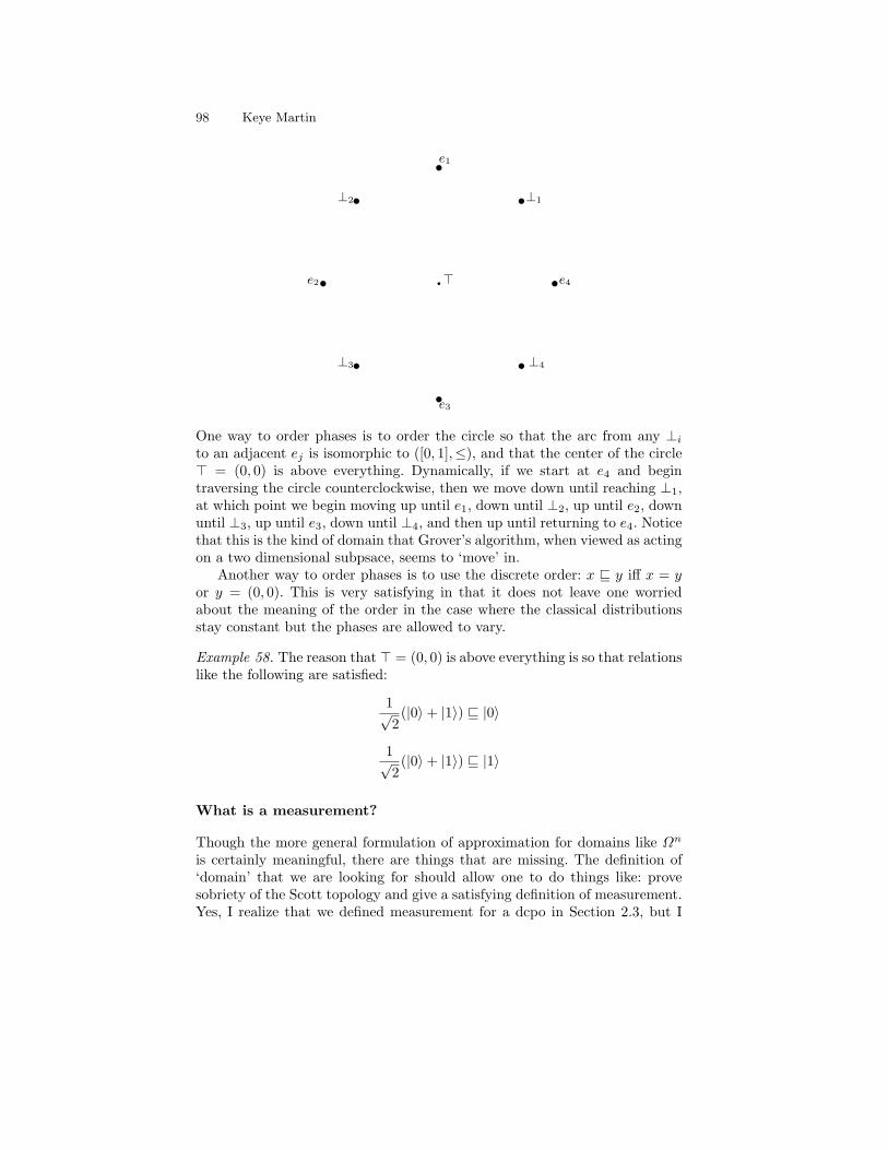
98 Keye Martin

q>

s⊥1

se1⊥2 s

se2

⊥3 sse3

s⊥4

se4

One way to order phases is to order the circle so that the arc from any ⊥ito an adjacent ej is isomorphic to ([0, 1],≤), and that the center of the circle> = (0, 0) is above everything. Dynamically, if we start at e4 and begintraversing the circle counterclockwise, then we move down until reaching ⊥1,at which point we begin moving up until e1, down until ⊥2, up until e2, downuntil ⊥3, up until e3, down until ⊥4, and then up until returning to e4. Noticethat this is the kind of domain that Grover’s algorithm, when viewed as actingon a two dimensional subpsace, seems to ‘move’ in.

Another way to order phases is to use the discrete order: x v y iff x = yor y = (0, 0). This is very satisfying in that it does not leave one worriedabout the meaning of the order in the case where the classical distributionsstay constant but the phases are allowed to vary.

Example 58. The reason that > = (0, 0) is above everything is so that relationslike the following are satisfied:

1√2

(|0〉+ |1〉) v |0〉

1√2

(|0〉+ |1〉) v |1〉

What is a measurement?

Though the more general formulation of approximation for domains like Ωn

is certainly meaningful, there are things that are missing. The definition of‘domain’ that we are looking for should allow one to do things like: provesobriety of the Scott topology and give a satisfying definition of measurement.Yes, I realize that we defined measurement for a dcpo in Section 2.3, but I


never said that we found the definition entirely convincing. The definition ofmeasurement has more impact on a continuous dcpo as evidenced by resultslike Theorems 2 and 3.

Related to this question are two more pressing issues: (a) systematic meth-ods for deriving higher order measurements from simpler measurements, and(b) techniques for proving that a given function is a measurement. For in-stance, to illustrate (a), if D is a domain and F (D) is some higher orderdomain, like a powerdomain or an exponential object, can a measurement onD be used to simply construct one on F (D)? The question (b) is particularlyurgent in physics and information theory: generally speaking, proving thatfunctions like entropy and capacity are measurements is about as much funas being a domain theorist in search of a decent job4.

References

1. Abramsky, S. and Jung, A. (1994) Domain theory. In In S. Abramsky, D.M. Gabbay, T. S. E. Maibaum (editors), Handbook of Logic in ComputerScience III, Oxford University Press.

2. P. M. Alberti and A. Uhlmann. Stochasticity and partial order: doublystochastic maps and unitary mixing. Dordrecht, Boston, 1982.

3. R. P. Brent, Algorithms for minimization without derivatives. Prentice-Hall,1973.

4. F. L. Chernous’ko, An optimal algorithm for finding the roots of an approx-imately computed function. Zh. vychisl. Mat. i mat. Fiz. 8, 4, p. 705–724,1968, English translation.

5. B. Coecke and K. Martin. A partial order on classical and quantum states.Oxford University Computing Laboratory Research Report, August 2002.

6. Edalat, A. and Heckmann, R. (1998) A computational model for metricspaces. Theoretical Computer Science 193, 53–73.

7. K. Falconer, Fractal geometry. John Wiley and Sons, 1990.8. O. Gross and S. M. Johnson, Sequential minimax search for a zero of a

convex function. Mathematical Tables and Other Aids to Computation,Vol. 13, Issue 65, p. 44–51, 1959.

9. L. K. Grover. Quantum mechanics helps in searching for a needle in ahaystack. Physical Review Letters, 78:325, 1997.

10. S.W. Hawking and G.F.R. Ellis. The large scale structure of space-time.Cambridge Monographs on Mathematical Physics. Cambridge UniversityPress, 1973.

11. Hutchinson, J. E. (1981) Fractals and self-similarity. Indiana UniversityMathematics Journal 30, 713–747.

12. M. Kowalski, K. Sikorski and F. Stenger, Selected topics in approximationand computation. Oxford University Press, 1995.

13. L. G. Kraft. A device for quantizing, grouping and coding amplitude modu-lated pulses. M.S. Thesis, Electrical Engineering Department, MIT, 1949.

4 Any such domain theorist should send a CV and some recent papers [email protected] immediately.

100 Keye Martin

14. A. W. Marshall and I. Olkin. Inequalities: Theory of majorization and itsapplications. Academic Press Inc., 1979.

15. K. Martin (2000) A foundation for computation. Ph.D. Thesis, Tulane Uni-versity, Department of Mathematics.

16. K. Martin. The measurement process in domain theory. Lecture Notes InComputer Science, Vol. 1853, Springer-Verlag, 2000.

17. K. Martin (2001) Unique fixed points in domain theory. Electronic Notesin Theoretical Computer Science.

18. K. Martin (2001) A renee equation for algorithmic complexity, LectureNotes in Computer Science, Springer-Verlag, Volume 2215.

19. K. Martin. Powerdomains and zero finding. Electronic Notes in TheoreticalComputer Science, Vol. 59(3), 2001.

20. K. Martin. The informatic derivative at a compact element. Lecture Notesin Computer Science, Vol. 2303, Springer-Verlag, 2002.

21. K. Martin, B-sides. Oxford University Computing Lab, Research Report,2003.

22. K. Martin. Epistemic motion in quantum searching. Oxford UniversityComputing Laboratory, Research Report, 2003.

23. K. Martin. A continuous domain of classical states. Oxford University Com-puting Laboratory, Research Report, 2003.

24. K. Martin (2004) Fractals and domain theory. Mathematical Structures inComputer Science, Volume 14, Issue 6, p. 833–851, Cambridge UniversityPress.

25. K. Martin and J. Ouaknine. Informatic vs. classical differentiation on thereal line. Electronic Notes in Theoretical Computer Science, Vol. 73, 2004.

26. K. Martin and P. Panangaden. A domain of spacetime intervals in gen-eral relativity. Communications in Mathematical Physics, 267(3):563–586,November 2006.

27. K. Martin. Compactness of the space of causal curves. Journal of Classicaland Quantum Gravity, 2006.

28. K. Martin. Entropy as a fixed point. Theoretical Computer Science, 2006.29. K. Martin (2007) Topology in information theory in topology. Theoretical

Computer Science, to appear.30. K. Martin. A domain theoretic model of qubit channels. To appear, 2008.31. K. Martin. The maximum entropy state. Logical Methods in Computer

Science, to appear.32. K. Martin and P. Panangaden. In preparation. 2008.33. J. Mashburn. A spectral order for infinite dimensional quantum spaces.

Electronic Notes in Theoretical Computer Science, Volume 173, 2007.34. R. F. Muirhead. Some methods applicable to identities and inequalities of

symmetric algebraic functions of n letters. Proc. Edinburgh Math. Soc.,21:144-157, 1903.

35. M. Nielsen and I. Chuang, Quantum computation and quantum informa-tion. Cambridge University Press, 2000.

36. Roger Penrose. Gravitational collapse and space-time singularities. Phys.Rev. Lett., 14:57–59, 1965.

37. Roger Penrose. Techniques of differential topology in relativity. Society forIndustrial and Applied Mathematics, 1972.

38. H. L. Royden, Real analysis. Third Edition, Macmillan Publishing, 1988.


39. E. Schrodinger. Proceedings of the Cambridge Philosophical Society 32,446 (1936).

40. D. Scott. Outline of a mathematical theory of computation. Technical Mono-graph PRG-2, Oxford University Computing Laboratory, November 1970.

41. C. E. Shannon. A mathematical theory of communication. Bell SystemsTechnical Journal 27, 379–423 and 623–656, 1948.

42. R. Sorkin. Spacetime and causal sets. In J. D’Olivo et. al., editor, Relativityand Gravitation: Classical and Quantum. World Scientific, 1991.

43. D. Spreen (2001) On some constructions in quantitative domain theory.Extended Abstract. http://www.informatik.uni-siegen.de/ spreen/

44. R.M. Wald. General relativity. The University of Chicago Press, 1984.45. P. Waszkiewicz. Quantitative continuous domains. PhD Thesis, University

of Birmingham, 2002.46. M. Yamaguti, M. Hata and J. Kigami, Mathematics of fractals. Translations

of Mathematical Monographs, American Math Society, vol. 167, 1997.

domain theory and measurement

Documents