Domain Theory, Testing and Simulation for

Labelled Markov Processes

Franck van Breugel a,4, Michael Mislove b,1,3, Joel Ouaknine c,2,James Worrell b,1,3

aYork University, Department of Computer Science, 4700 Keele Street, TorontoM3J 1P3, Canada

bDepartment of Mathematics, Tulane University, 6823 St Charles Avenue, NewOrleans LA 70118, USA

cComputer Science Department, Carnegie Mellon University, 5000 Forbes Avenue,Pittsburgh PA 15213, USA

Abstract

This paper presents a fundamental study of similarity and bisimilarity for labelledMarkov processes. The main results characterize similarity as a testing preorder andbisimilarity as a testing equivalence. In general, labelled Markov processes are notrequired to satisfy a finite-branching condition—indeed the state space may be acontinuum, with the transitions given by arbitrary probability measures. Neverthe-less we show that to characterize bisimilarity it suffices to use finitely-branchinglabelled trees as tests.

Our results involve an interaction between domain theory and measure theory.One of the main technical contributions is to show that a final object in a suit-able category of labelled Markov processes can be constructed by solving a domainequation D ∼= V(D)Act, where V is the probabilistic powerdomain. Given a labelledMarkov process whose state space is an analytic space, bisimilarity arises as the ker-nel of the unique map to the final labelled Markov process. We also show that themetric for approximate bisimilarity introduced by Desharnais, Gupta, Jagadeesanand Panangaden generates the Lawson topology on the domain D.

1 The support of the US Office of Naval Research is gratefully acknowledged.2 Supported by ONR contract N00014-95-1-0520, Defense Advanced ResearchProject Agency and the Army Research Office under contract DAAD19-01-1-0485.3 The support of the National Science Foundation is gratefully acknowledged.4 Supported by the Natural Sciences and Engineering Research Council of Canada.

Preprint submitted to Elsevier Science 29 April 2005

1 Introduction

It is a notable feature of concurrency theory that there are many different no-tions of process equivalence. These are often presented in an abstract manner,e.g., using coinduction or domain theory. Ultimately, however, one would liketo know that any proposed notion of equivalence has some interpretation interms of the observable behaviour of a process. One way of formalizing thisis via a testing framework [1,5,20]. The idea is to specify an interaction be-tween a tester and the process. The latter is seen as a black box, with hiddeninternal state, and an interface consisting of buttons by which the tester maycontrol the execution of the process. If the tester cannot distinguish two pro-cesses, then they are deemed equivalent. By varying the power of the tester onerecovers different equivalences and preorders, e.g., trace equivalence, failuresequivalence, simulation, bisimulation, etc. In some cases a testing frameworkcan be used to give a denotational semantics, where the meaning of a processis a function from tests to observations.

This paper presents a testing framework characterizing similarity and bisim-ilarity for labelled Markov processes (LMPs). One can view LMPs as prob-abilistic versions of labelled transition systems from concurrency theory, or,alternatively, as indexed collections of discrete-time Markov processes in thesense of classical probability theory. More precisely, a labelled Markov processconsists of a measurable space (X, Σ) of states, a family Act of actions, and,for each a ∈ Act, a transition probability function µ−,a that, given a statex ∈ X, yields the probability µx,a(A) that the next state of the process willbe in the measurable set A ∈ Σ after performing action a.

Probabilistic models have been studied for quite a while in automata theoryand in formal verification, but, for understanding our concerns, the paper ofLarsen and Skou [20] is a good starting point. In particular, Larsen and Skouadapted the notion of bisimilarity to discrete probabilistic labelled transitionsystems. They defined an equivalence relation R on the states of a systemto be a bisimulation if related states have exactly matching probabilities ofmaking a transition into any given R-equivalence class. The two main resultsof [20] characterize bisimilarity as, respectively, equivalence with respect to aprobabilistic version of Hennessy-Milner logic, and equivalence with respectto a class of tests similar to those of Abramsky [1] and Bloom and Meyer [5].

Larsen and Skou’s probabilistic transition systems are LMPs with discretetransition probabilities. Desharnais, Edalat and Panangaden [9] extended thenotion of bisimilarity to LMPs with arbitrary transition probabilities, andgave a suite of examples motivating the more general model. The main re-sult of [9] is an extension of the logical characterization of bisimilarity to thegeneral setting. In fact, they used a simpler logic than Larsen and Skou—a

2

logic without disjunction. In another paper, Desharnais, Gupta, Jagadeesanand Panangaden [12] gave a logical characterization of similarity of LMPs,showing that, in this case, disjunction is essential.

In this paper we generalize the other main result of [20]—the characterizationof bisimilarity as a testing equivalence—to the LMP model. Our results followan intriguingly similar pattern to those of [9,12]. In particular, we find that wecan simplify the class of tests used by Larsen and Skou to characterize bisim-ilarity. This validates an intuition of [9] that working with LMPs providesthe right level of generality for developing the basic theory of probabilisticbisimilarity—even if ultimately one is only interested in discrete systems. Fur-thermore, and similarly to [12], we find that to characterize similarity, we needto enrich the set of tests with a kind of disjunction. We discuss the parallelbetween our results and those of [9,12] at greater length in the conclusion.

The tests that we use to characterize bisimilarity are technically just finitetrees whose edges are labelled by actions—in other words, traces with branchpoints. Two states of an LMP are bisimilar just in case they pass each testwith the same probability. In order to capture similarity, we need to consider amore structured class of trees, where the nodes are labelled with propositionalformulas. This provides both a conjunctive and disjunctive mode of combiningtests. We show that one state of a process simulates another state just in caseit passes each test with a higher probability.

Although we regard the testing results as the highlight of the present paper,they do not appear until Section 8. The main body of this work is concernedwith a domain-theoretic analysis of LMPs, upon which the results of Sec-tion 8 ultimately depend. The central mathematical construction here is thederivation of a final LMP as the solution of a domain equation involving theprobabilistic powerdomain. The same domain equation was studied in [12],where its status as a universal LMP was also described. However, while theconstruction is the same, we a give a different, functorial justification of theuniversal property. We also contribute a new result by relating the Lawsontopology on the universal LMP with the metric for approximate bisimilarityof LMPs from [6,10]. In particular, this shows that the class of all LMPs iscompact with respect to this metric.

Next we give, section by section, a summary of the contents of the paper.

Section 2 presents some preliminary notions from domain theory and measuretheory.

In Section 3 we formally introduce LMPs and the appropriate morphismsbetween them: zig-zag maps. While bisimulations could simply be defined tobe the kernels of zig-zag maps, following [12] we show that for an LMP whosestate space is analytic there is a less abstract relational characterization.

3

After introducing the probabilistic powerdomain V(D) in Section 4, in Section5 we investigate the Lawson topology on V(D), characterizing it as a weaktopology in the sense of measure theory. This yields another proof of the resultof Jung and Tix [19] that the probabilistic powerdomain of a coherent domainis itself coherent.

In Section 6 we show that the canonical solution of the domain equationD ∼= V(D)Act can be given the structure of a final LMP. The significance ofthis construction is that we can reduce questions about LMPs in general toquestions about the domain D—and so take advantage of certain nice prop-erties of D, like Lawson compactness.

In order to study bisimilarity on an LMP, Desharnais, Gupta, Jagadeesanand Panangaden [10] introduce a kind of dual space: a certain lattice of mea-surable functions on the state space. In Section 7, applying the reductiontechnique alluded to above, we study this class of functions in the case of thefinal LMP. In this case the given functions are all Lawson continuous. Usingthis observation we show that two states of an LMP are bisimilar iff theyare indistinguishable by functions in the dual space. This result is the foun-dation for our main theorems concerning testing. These theorems are provenin Section 8.

2 Preliminaries

In this section we outline some basic definitions and results from domaintheory and from measure theory. This is intended as a convenient summaryfor the reader. A more detailed treatment of the relevant domain theory andmeasure theory can be found respectively in Gierz et al. [15] and Arveson [4].

2.1 Domain Theory

Let (P,v) be a poset. Given A ⊆ P , we write ↑A for the set {x ∈ P | (∃a ∈A) a v x}; similarly, ↓A denotes {x ∈ P | (∃a ∈ A) x v a}. A directedcomplete partial order (dcpo) is a poset P in which each directed set A has aleast upper bound, denoted tA. If P is a dcpo, and x, y ∈ P , then we writex � y if each directed subset A ⊆ D with y v tA satisfies ↑x ∩ A 6= ∅.We then say x is way-below y. Let ↓↓y = {x ∈ D | x � y}; we say that P iscontinuous if it has a basis, i.e., a subset B ⊆ P such that for each y ∈ P ,

↓↓y ∩ B is directed with supremum y. We use the term domain to mean acontinuous dcpo. If a continuous dcpo has a countable basis we say that it isω-continuous.

4

A subset U of a domain D is Scott open if it is an upper set (i.e., U = ↑U)and for each directed set A ⊆ D, if tA ∈ U then A ∩ U 6= ∅. The collectionσD of all Scott-open subsets of D is called the Scott topology on D. If D iscontinuous, then the Scott topology on D is locally compact, and the sets↑↑x where x ∈ D form a basis for this topology. Given domains D and E, afunction f : D → E is continuous with respect to the Scott topologies on Dand E iff it is monotone and preserves directed suprema: for each directedA ⊆ D, f(tA) = tf(A).

In fact the topological and order-theoretic views of a domain are interchange-able. The order on a domain can be recovered from the Scott topology as thespecialization preorder. Recall that for a topological space X the specializationpreorder 6⊆ X ×X is defined by x 6 y iff x ∈ Cl(y).

Another topology of interest on a domain D is the Lawson topology. This isthe join of the Scott topology and the lower interval topology, where the latteris generated by sub-basic open sets of the form D \ ↑x. Thus, the Lawsontopology has the family {↑↑x \ ↑F | x ∈ D,F ⊆ D finite} as a basis. TheLawson topology on a domain is always Hausdorff. A domain that is compactin its Lawson topology is called coherent.

2.2 Measure Theory

Recall that a σ-field Σ on a set X is a collection of subsets of X containing ∅and closed under complements and countable unions. The pair 〈X, Σ〉 is calleda measurable space. For any collection C of subsets on X there is a smallestσ-field containing C, written σ(C). In case X is a topological space and C isthe class of open subsets, then σ(C) is called the Borel σ-field on X. One cansplit the definition of a σ-field into two steps. A collection of subsets of X iscalled a π-system if it closed under finite intersections. A collection of subsetsof X closed under countable disjoint unions, complements, and containing theempty set is called a λ-system. The π − λ theorem [14] states that if P is aπ-system, L is a λ-system, and P ⊆ L, then σ(P) ⊆ L.

If Σ = σ(C) for some countable set C, then we say that Σ is countably generated.We say that (X, Σ) is countably separated if there is a countable subset C ⊆ Σsuch that no two distinct elements of X lie in precisely the same membersof C. A topological space is a Polish space if it is separable and completelymetrizable.

Given a measurable space 〈X, Σ〉, we say that A ⊆ X is (Σ-)measurable ifA ∈ Σ. If 〈X ′, Σ′〉 is another measurable space, a function f : X → X ′ is saidto be measurable if f−1(A) ∈ Σ for each A ∈ Σ′. Measurable spaces andfunctions form a category Mes. The limit of a diagram in Mes in obtained by

5

equipping the limit of the underlying diagram in the category of sets with thesmallest σ-field structure making all the projections measurable.

A function µ : Σ→ [0, 1] is a sub-probability measure on 〈X, Σ〉 if µ(⋃

n An) =∑

n µ(An) for any countable family of pairwise disjoint measurable sets {An}.

3 Labelled Markov Processes

Assume a fixed countable set Act of actions or labels. A labelled Markovprocess is just an Act-indexed family of Markov processes on the same statespace.

Definition 1 A labelled Markov process (LMP) is a triple 〈X, Σ, µ〉 consist-ing of a set X of states, a σ-field Σ on X, and a transition probability functionµ : X × Act× Σ→ [0, 1] such that

(1) for all x ∈ X and a ∈ Act, the function µx,a(·) : Σ → [0, 1] is a sub-probability measure, and

(2) for all a ∈ Act and A ∈ Σ, the function µ−,a (A) : X → [0, 1] is measur-able.

This is the so-called reactive model of probabilistic processes. The functionµ−,a describes the reaction of the process to the action a selected by theenvironment. Given that the process is in state x and action a is selected,µx,a(A) is the probability that the process makes a transition to a state in A.Note that we consider subprobability measures, i.e., positive measures withtotal mass no greater than 1. We interpret 1 − µx,a(X) as the probability ofrefusing action a in state x. In fact, if every transition measure had mass 1,then all processes would be bisimilar (cf. Definition 3).

An important special case is when the σ-field Σ is taken to be the powersetof X. Then, for all actions a and states x, the sub-probability measure µx,a(·)is completely determined by a discrete sub-probability distribution. This casecorresponds to the original probabilistic transition system model of Larsenand Skou [20].

A natural notion of a map between labelled Markov processes is given in:

Definition 2 Given labelled Markov processes 〈X, Σ, µ〉 and 〈X ′, Σ′, µ′〉, ameasurable function f : X → X ′ is called a zig-zag map if whenever A′ ∈Σ′, x ∈ X, and a ∈ Act, then µx,a(f

−1(A′)) = µ′f(x),a(A

′).

Probabilistic bisimulations (henceforth just bisimulations) are the relationalcounterparts of zig-zag maps, and can also be seen, in a very precise way,

6

as the probabilistic analogues of the strong bisimulations of Park and Milner[21]. They were first introduced in the discrete case by Larsen and Skou [20].The notion of bisimulation was extended to LMPs in [9,12]. (Though ourformulation is slightly different as we explain below.)

Definition 3 Let 〈X, Σ, µ〉 be a labelled Markov process and R a reflexiverelation on X. For A ⊆ X, write R(A) for the image of A under R. We saythat R is a simulation if it satisfies condition (i) below, and we say that R isa bisimulation if it satisfies both conditions (i) and (ii).

(i) xRy ⇒ (∀a ∈ Act)(∀A ∈ Σ)(A = R(A)⇒ µx,a(A) 6 µy,a(A)).(ii) xRy ⇒ (∀a ∈ Act)(µx,a(X) = µy,a(X)).

We say that two states are (bi)similar if they are related by some (bi)simulation.

The notions of simulation and bisimulation are very close, reflecting the factthat LMPs are like deterministic systems. The extra condition µx,a(X) =µy,a(X) in the definition of bisimulation can be seen as a ‘readiness’ condition:related states perform given actions with the same probability. It may not beimmediately apparent that the notion of bisimulation is symmetric, howeverthis fact is straightforward, as we now show.

Proposition 4 Suppose R is a bisimulation on a labelled Markov process〈X, Σ, µ〉. Then the inverse R−1 is also a bisimulation.

PROOF. Given x, y ∈ X, A ∈ Σ and a ∈ Act, we have the following chainof implications.

xR−1y and A = R−1(A)⇒ yRx and X \ A = R(X \ A)

⇒µy,a(X \ A) 6 µx,a(X \ A)

⇒µx,a(X)− µx,a(X \ A) 6 µy,a(X)− µy,a(X \ A)

⇒µx,a(A) 6 µy,a(A).

2

It is straightforward that the relational composition of two bisimulations on〈X, Σ, µ〉 is again a bisimulation and that the union of any family of bisim-ulations is a bisimulation. In particular, there is a largest bisimulation on〈X, Σ, µ〉 and it is an equivalence relation. For an equivalence relation R thetwo criteria in Definition 3 can be compressed into the following more intuitivecondition:

xRy ⇒ (∀a ∈ Act)(∀A ∈ Σ)(A = R(A)⇒ µx,a(A) = µy,a(A)) .

7

In words: related states have matching probabilities of jumping into any mea-surable block of equivalence classes. This is actually the definition of bisimu-lation in [9].

Propositions 5 and 8 below make precise the connection between bisimulationsand zig-zag maps. These results are implicit in [9], and our proofs recapitulatearguments from there. The one novelty below is in our use of the existenceof a final LMP whose state space is a Polish space. This plays a similar roleto the countable logic characterizing bisimilarity from [9]. We spell out thissmall variation in order to make our paper more self-contained.

Proposition 5 Every bisimulation equivalence is the kernel of a zig-zag map.

PROOF. Given a measurable space 〈X, Σ〉 and an equivalence relation R onX, let ΣR be the greatest σ-field on the set of R-equivalence classes X/R suchthat the quotient map q : X → X/R is measurable. Thus ΣR = {E | q−1(E) ∈Σ}. Now if 〈X, Σ, µ〉 is an LMP and R is a bisimulation, it is easy to see that

µR : X/R× Act× ΣR → [0, 1]

defined by (µR)[x],a(E) = µx,a(q−1(E)) is well-defined and is the unique tran-

sition probability function making q a zig-zag map. 2

To prove a converse to Proposition 5 we need to use the following two resultsabout analytic measurable spaces. A measurable space is said to be analyticif it is the image of a measurable map from one Polish space to another.

Theorem 6 (Corollary 3.3.1[4]) Let f : 〈X, Σ〉 → 〈X ′, Σ′〉 be a surjectivemeasurable map, where 〈X, Σ〉 is analytic and 〈X ′, Σ′〉 is countably separated.Then 〈X ′, Σ′〉 is also analytic.

Theorem 7 (Theorem 3.3.5[4]) If 〈X, Σ〉 is an analytic measurable spaceand Σ0 a countably generated sub-σ-field of Σ that separates points in X (givenx, y ∈ X with x 6= y, there exists A ∈ Σ0 with x ∈ A and y 6∈ A), then Σ0 = Σ.

The importance of analycity in the present context was first realized in [9].We do not know if the result below is true without such an assumption.

Proposition 8 Given a zig-zag map f : 〈X, Σ, µ〉 → 〈X ′, Σ′, µ′〉 with 〈X, Σ〉an analytic measurable space, the kernel of f is contained in a bisimulation.

PROOF. By Theorem 22 there is a final LMP whose state space is a Polishspace. Since the kernel of f is contained in the kernel of the unique zig-zag mapfrom 〈X, Σ, µ〉 to this final LMP we may, without loss of generality, assume

8

that 〈X ′, Σ′〉 is a Polish space. Let R ⊆ X × X denote the kernel of f , andq : 〈X, Σ〉 → 〈X/R, ΣR〉 the quotient map in Mes. It remains to show that Ris a bisimulation.

Consider the following two sub-σ-fields Σ1, Σ2 ⊆ Σ.

Σ1 = {f−1(A) | A ∈ Σ′}

Σ2 = {A ∈ Σ | A = R(A)}

It is straightforward that Σ1 ⊆ Σ2 ⊆ Σ. Observe also that q(Σ1) := {q(A) |A ∈ Σ1} and q(Σ2) := {q(A) | A ∈ Σ2} are both σ-fields on X/R with

q(Σ1) ⊆ q(Σ2) ⊆ ΣR .

But X/R is countably separated, being a subobject of the Polish space X ′,and so it is an analytic space by Theorem 6. From the fact that Σ′ is count-ably generated and separates points it is readily seen that q(Σ1) is count-ably generated and separates points in X/R. It follows from Theorem 7 thatq(Σ1) = q(Σ2) = ΣR and thence that Σ1 = Σ2.

Suppose x, y ∈ X are chosen such that xRy and E ⊆ X is an R-closed Σ-measurable set. Then E ∈ Σ2 by definition of Σ2, and so E ∈ Σ1, i.e., thereexists A ∈ Σ′ with E = f−1(A). Now given a ∈ Act,

µx,a(E) = µ′f(x),a(A) = µ′

f(y),a(A) = µy,a(E) .

2

4 The Probabilistic Powerdomain

We briefly recall some basic definitions and results about valuations and theprobabilistic powerdomain. For more details see Jones [18].

Definition 9 Let (X, τ) be a topological space. A valuation on X is a mappingµ : τ → [0, 1] satisfying:

• strictnessµ∅ = 0

• monotonicityU ⊆ V implies µU ⊆ µV

• modularityµ(U ∪ V ) + µ(U ∩ V ) = µU + µV for all U, V .

• Scott continuityµ(

⋃

i∈I Ui) = supi∈I µUi for every directed family {Ui}i∈I .

9

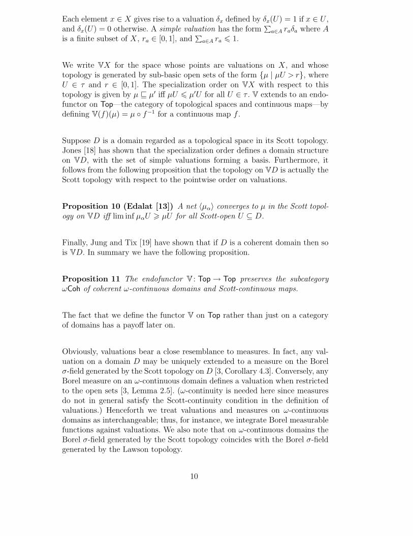
Each element x ∈ X gives rise to a valuation δx defined by δx(U) = 1 if x ∈ U ,and δx(U) = 0 otherwise. A simple valuation has the form

∑

a∈A raδa where Ais a finite subset of X, ra ∈ [0, 1], and

∑

a∈A ra 6 1.

We write VX for the space whose points are valuations on X, and whosetopology is generated by sub-basic open sets of the form {µ | µU > r}, whereU ∈ τ and r ∈ [0, 1]. The specialization order on VX with respect to thistopology is given by µ v µ′ iff µU 6 µ′U for all U ∈ τ . V extends to an endo-functor on Top—the category of topological spaces and continuous maps—bydefining V(f)(µ) = µ ◦ f−1 for a continuous map f .

Suppose D is a domain regarded as a topological space in its Scott topology.Jones [18] has shown that the specialization order defines a domain structureon VD, with the set of simple valuations forming a basis. Furthermore, itfollows from the following proposition that the topology on VD is actually theScott topology with respect to the pointwise order on valuations.

Proposition 10 (Edalat [13]) A net 〈µα〉 converges to µ in the Scott topol-ogy on VD iff lim inf µαU > µU for all Scott-open U ⊆ D.

Finally, Jung and Tix [19] have shown that if D is a coherent domain then sois VD. In summary we have the following proposition.

Proposition 11 The endofunctor V : Top→ Top preserves the subcategoryωCoh of coherent ω-continuous domains and Scott-continuous maps.

The fact that we define the functor V on Top rather than just on a categoryof domains has a payoff later on.

Obviously, valuations bear a close resemblance to measures. In fact, any val-uation on a domain D may be uniquely extended to a measure on the Borelσ-field generated by the Scott topology on D [3, Corollary 4.3]. Conversely, anyBorel measure on an ω-continuous domain defines a valuation when restrictedto the open sets [3, Lemma 2.5]. (ω-continuity is needed here since measuresdo not in general satisfy the Scott-continuity condition in the definition ofvaluations.) Henceforth we treat valuations and measures on ω-continuousdomains as interchangeable; thus, for instance, we integrate Borel measurablefunctions against valuations. We also note that on ω-continuous domains theBorel σ-field generated by the Scott topology coincides with the Borel σ-fieldgenerated by the Lawson topology.

10

5 The Lawson Topology on VD

Given an ω-continuous domain D, we define the weak topology 5 on VDto be the weakest topology such that for any Lawson-continuous functionf : D → [0, 1], the map µ 7→

∫

fdµ is continuous. An alternative characteriza-tion is that a net of valuations 〈µα〉 converges to µ in the weak topology ifflim inf µαO > µO for each Lawson-open set O (cf. [22, Thm II.6.1]). Next weshow that for a coherent domain D, the Lawson topology on VD coincideswith the weak topology.

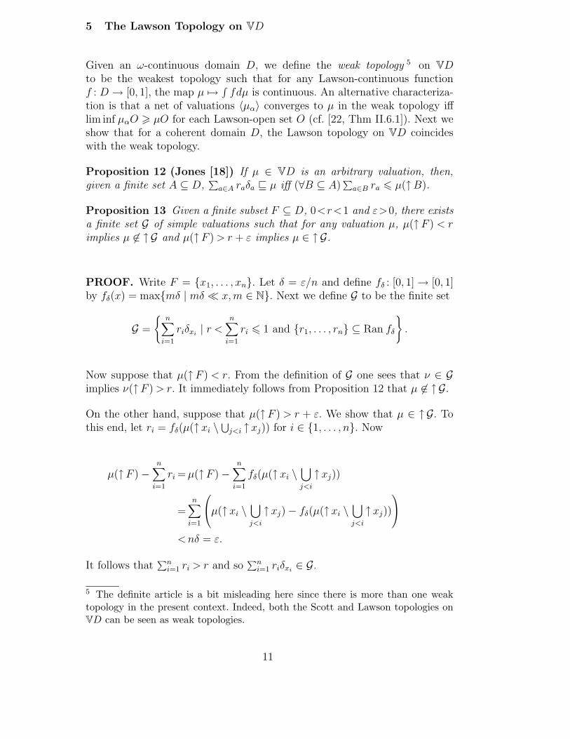
Proposition 12 (Jones [18]) If µ ∈ VD is an arbitrary valuation, then,given a finite set A ⊆ D,

∑

a∈A raδa v µ iff (∀B ⊆ A)∑

a∈B ra 6 µ(↑B).

Proposition 13 Given a finite subset F ⊆ D, 0<r<1 and ε>0, there existsa finite set G of simple valuations such that for any valuation µ, µ(↑F ) < rimplies µ 6∈ ↑ G and µ(↑F ) > r + ε implies µ ∈ ↑G.

PROOF. Write F = {x1, . . . , xn}. Let δ = ε/n and define fδ : [0, 1]→ [0, 1]by fδ(x) = max{mδ | mδ � x,m ∈ N}. Next we define G to be the finite set

G =

{

n∑

i=1

riδxi| r <

n∑

i=1

ri 6 1 and {r1, . . . , rn} ⊆ Ran fδ

}

.

Now suppose that µ(↑F ) < r. From the definition of G one sees that ν ∈ Gimplies ν(↑F ) > r. It immediately follows from Proposition 12 that µ 6∈ ↑ G.

On the other hand, suppose that µ(↑F ) > r + ε. We show that µ ∈ ↑G. Tothis end, let ri = fδ(µ(↑xi \

⋃

j<i ↑xj)) for i ∈ {1, . . . , n}. Now

µ(↑F )−n

∑

i=1

ri = µ(↑F )−n

∑

i=1

fδ(µ(↑xi \⋃

j<i

↑ xj))

=n

∑

i=1

µ(↑xi \⋃

j<i

↑ xj)− fδ(µ(↑xi \⋃

j<i

↑ xj))

<nδ = ε.

It follows that∑n

i=1 ri > r and so∑n

i=1 riδxi∈ G.

5 The definite article is a bit misleading here since there is more than one weaktopology in the present context. Indeed, both the Scott and Lawson topologies onVD can be seen as weak topologies.

11

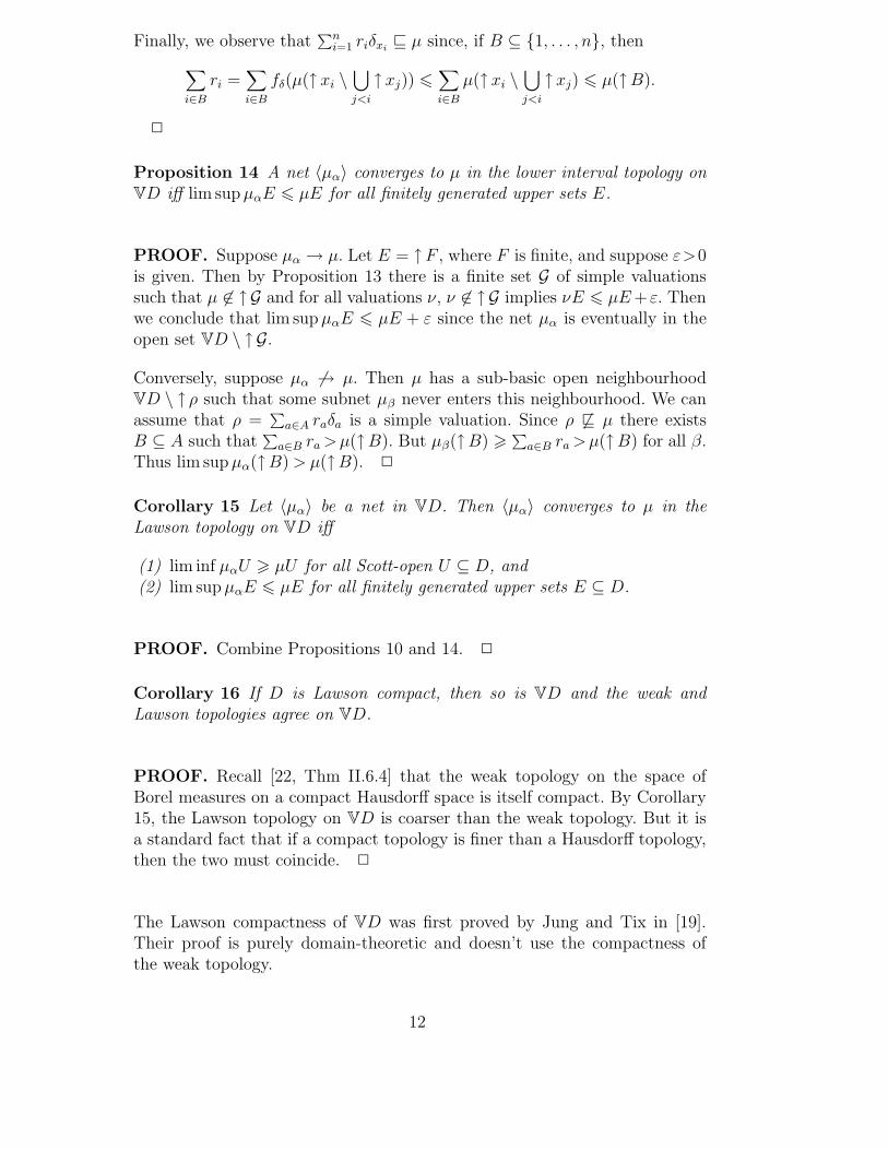
Finally, we observe that∑n

i=1 riδxiv µ since, if B ⊆ {1, . . . , n}, then

∑

i∈B

ri =∑

i∈B

fδ(µ(↑xi \⋃

j<i

↑ xj)) 6∑

i∈B

µ(↑xi \⋃

j<i

↑ xj) 6 µ(↑B).

2

Proposition 14 A net 〈µα〉 converges to µ in the lower interval topology onVD iff lim sup µαE 6 µE for all finitely generated upper sets E.

PROOF. Suppose µα → µ. Let E = ↑F , where F is finite, and suppose ε>0is given. Then by Proposition 13 there is a finite set G of simple valuationssuch that µ 6∈ ↑ G and for all valuations ν, ν 6∈ ↑ G implies νE 6 µE + ε. Thenwe conclude that lim sup µαE 6 µE + ε since the net µα is eventually in theopen set VD \ ↑ G.

Conversely, suppose µα 6→ µ. Then µ has a sub-basic open neighbourhoodVD \ ↑ ρ such that some subnet µβ never enters this neighbourhood. We canassume that ρ =

∑

a∈A raδa is a simple valuation. Since ρ 6v µ there existsB ⊆ A such that

∑

a∈B ra >µ(↑B). But µβ(↑B) >∑

a∈B ra >µ(↑B) for all β.Thus lim sup µα(↑B) > µ(↑B). 2

Corollary 15 Let 〈µα〉 be a net in VD. Then 〈µα〉 converges to µ in theLawson topology on VD iff

(1) lim inf µαU > µU for all Scott-open U ⊆ D, and(2) lim sup µαE 6 µE for all finitely generated upper sets E ⊆ D.

PROOF. Combine Propositions 10 and 14. 2

Corollary 16 If D is Lawson compact, then so is VD and the weak andLawson topologies agree on VD.

PROOF. Recall [22, Thm II.6.4] that the weak topology on the space ofBorel measures on a compact Hausdorff space is itself compact. By Corollary15, the Lawson topology on VD is coarser than the weak topology. But it isa standard fact that if a compact topology is finer than a Hausdorff topology,then the two must coincide. 2

The Lawson compactness of VD was first proved by Jung and Tix in [19].Their proof is purely domain-theoretic and doesn’t use the compactness ofthe weak topology.

12

6 A Final Labelled Markov Process

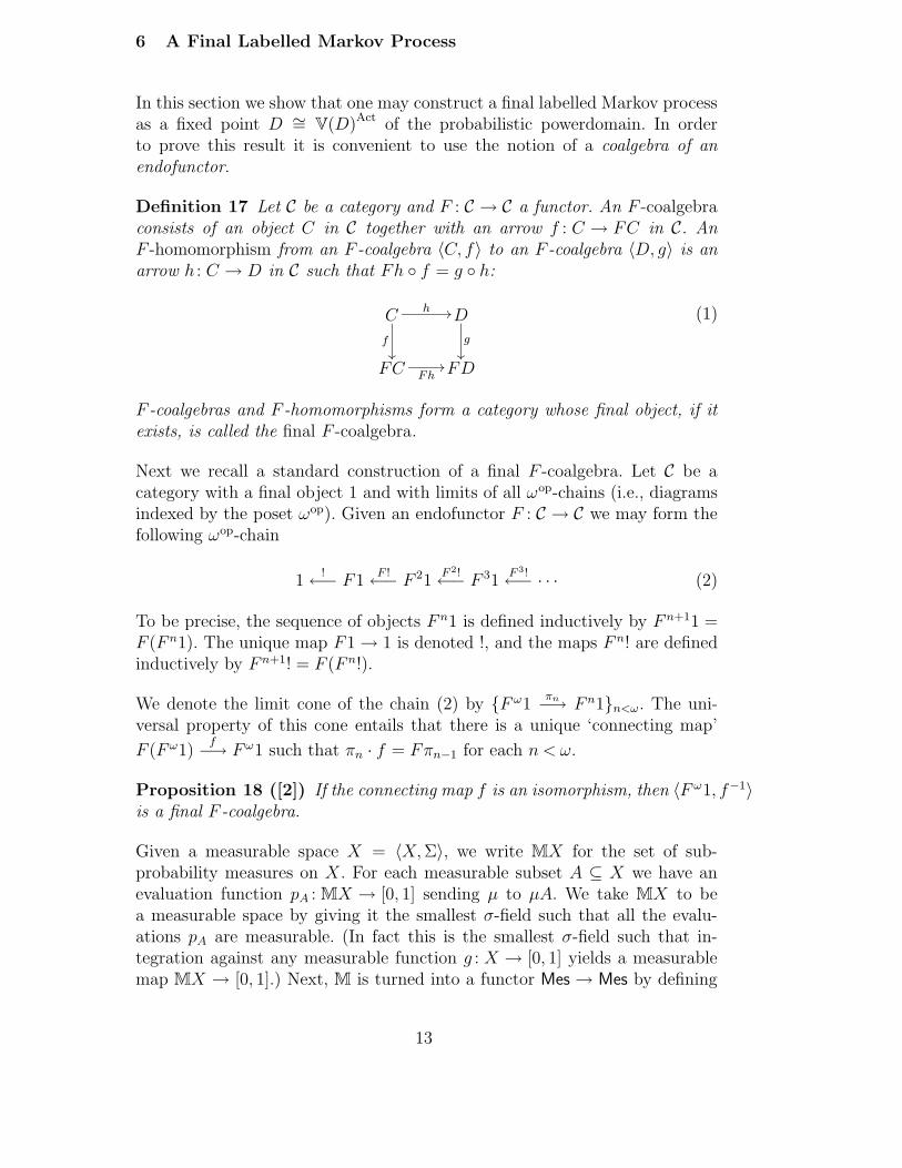
In this section we show that one may construct a final labelled Markov processas a fixed point D ∼= V(D)Act of the probabilistic powerdomain. In orderto prove this result it is convenient to use the notion of a coalgebra of anendofunctor.

Definition 17 Let C be a category and F : C → C a functor. An F -coalgebraconsists of an object C in C together with an arrow f : C → FC in C. AnF -homomorphism from an F -coalgebra 〈C, f〉 to an F -coalgebra 〈D, g〉 is anarrow h : C → D in C such that Fh ◦ f = g ◦ h:

C

f

��

h //Dg

��

FC Fh//FD

(1)

F -coalgebras and F -homomorphisms form a category whose final object, if itexists, is called the final F -coalgebra.

Next we recall a standard construction of a final F -coalgebra. Let C be acategory with a final object 1 and with limits of all ωop-chains (i.e., diagramsindexed by the poset ωop). Given an endofunctor F : C → C we may form thefollowing ωop-chain

1!←− F1

F !←− F 21

F 2!←− F 31

F 3!←− · · · (2)

To be precise, the sequence of objects F n1 is defined inductively by F n+11 =F (F n1). The unique map F1→ 1 is denoted !, and the maps F n! are definedinductively by F n+1! = F (F n!).

We denote the limit cone of the chain (2) by {F ω1πn−→ F n1}n<ω. The uni-

versal property of this cone entails that there is a unique ‘connecting map’

F (F ω1)f−→ F ω1 such that πn · f = Fπn−1 for each n < ω.

Proposition 18 ([2]) If the connecting map f is an isomorphism, then 〈F ω1, f−1〉is a final F -coalgebra.

Given a measurable space X = 〈X, Σ〉, we write MX for the set of sub-probability measures on X. For each measurable subset A ⊆ X we have anevaluation function pA : MX → [0, 1] sending µ to µA. We take MX to bea measurable space by giving it the smallest σ-field such that all the evalu-ations pA are measurable. (In fact this is the smallest σ-field such that in-tegration against any measurable function g : X → [0, 1] yields a measurablemap MX → [0, 1].) Next, M is turned into a functor Mes → Mes by defining

13

M(f)(µ) = µ ◦ f−1 for f : X → Y and µ ∈ MX. This functor is studied byGiry [16].

Given a labelled Markov process 〈X, Σ, µ〉, the transition probability functionµ may be regarded as a measurable map X →M(X)Act, where (−)Act denotesAct-fold product in Mes. That is, labelled Markov processes are nothing butcoalgebras of the endofunctor MAct on the category Mes. Furthermore it iseasy to verify that the coalgebra homomorphisms are precisely the zig-zagmaps.

Next, we relate the functor M to the probabilistic powerdomain functor V.To mediate between domains and measure spaces we introduce the forgetfulfunctor U : ωCoh→ Mes which maps a coherent domain to the Borel measur-able space generated by the Scott topology. Note in passing that the σ-fieldunderlying UD is also the Borel σ-field with respect to the Lawson topologyon D, and can thus be regarded as the Borel σ-field on a Polish space.

Proposition 19 M ◦ U = U ◦ V.

PROOF. Suppose D is a coherent domain with a countable basis. Sincevaluations on D in its Scott topology are in one-to-one correspondence withBorel sub-probability measures on U(D), we have a bijection between thepoints of the measurable spaces MU(D) and UV(D). It remains to show thatthe underlying σ-field structures are the same.

Since D is ω-continuous, the Scott topology on D is separable, and we maychoose a countable basis P of Scott-open sets that is closed under finite in-tersections and finite unions. The set of Borel sub-probability measures on Dcan be given a σ-field structure in the following ways.

Σ1 is the smallest σ-field such that pA is measurable for each Borel setA ⊆ D. This is the σ-field underlying MU(D).Σ2 is the smallest σ-field such that pA is measurable for each A ∈ P .Σ3 is the Borel σ-field generated by the Scott topology on VD. This is theσ-field underlying UV(D).

To complete the proof of the proposition we show that Σ1 = Σ2 = Σ3.

• Σ1 = Σ2. Clearly Σ2 ⊆ Σ1. For the converse, consider

L = {A ⊆ D | pA is Σ2-measurable}.

L is a λ-system, i.e., it is closed under countable disjoint unions, comple-ments and it contains D. Also, by definition of Σ2, we have that P is aπ-system contained in L. By the λ − π theorem we have that L contains

14

the σ-field generated by P ; but this is the whole Borel σ-field on D. ThusΣ1 ⊆ Σ2 by minimality of Σ1.• Σ2 = Σ3. Given A ∈ P , the evaluation map pA : VD → [0, 1] is Scott contin-

uous and thus Σ3-measurable. By minimality of Σ2 it follows that Σ2 ⊆ Σ3.Conversely, Σ2 is generated by sets {µ | µA > q} for A ∈ P and q ∈ Q. Butthis is a countable basis for the Scott topology on VD; thus Σ2 contains allScott-open sets, and Σ3 ⊆ Σ2 by minimality of Σ3. 2

The following proposition collects together some standard facts about limitsin Mes and ωCoh. For this reason we do not give a detailed proof, though weexplain the significance of the hypotheses and give pointers to the literature.

Proposition 20 (i) ωCoh is closed under countable products of pointed do-mains.

(ii) ωCoh is closed under limits of ωop-chains where the chain maps are Scott-continuous upper adjoints.

(iii) U preserves the limits in (i) and (ii).

PROOF. Limits in the category of dcpos and Scott-continuous functions arecreated by the forgetful functor to the category of sets (via the pointwiseorder) [15, Proposition IV-4.3]. The full subcategory ωCoh is not in generalclosed under such limits; however it is closed under countable products ofpointed domains [17, Lemma VII-3.1] and ωop-limits where the bonding mapsare Scott-continuous upper adjoints [15, Exercise IV-4.15].

Part (iii) follows from the conjunction of two standard facts. Firstly, the rel-evant limits in ωCoh are also limits in Top, where domains are regarded astopological spaces in their Scott topology. Next, the forgetful functor from Top

to Mes preserves countable limits of separable spaces (see, e.g., [22, Theorem1.10]). 2

Starting with the final object 1 of ωCoh, we construct the chain

1!←− VAct1

VAct!←− (VAct)21

(VAct)2!←− (VAct)31

(VAct)3!←− · · · (3)

and write {(VAct)ω1πn−→ (VAct)n1}n<ω for the limit cone. The map VAct1

!→ 1

has a lower adjoint since VAct1 has a least element. Thus each bonding mapin (3) has a lower adjoint.

Proposition 21

15

(i) The image of (3) under U : ωCoh→ Mes is the chain

1!←−MAct1

MAct!←− (MAct)21

(MAct)2!←− (MAct)31←− · · · (4)

similarly obtained by iterating the functor M.(ii) U((VAct)ω1) = (MAct)ω1.(iii) The image of the connecting map VAct((VAct)ω1)→ (VAct)ω1 under U is

the connecting map MAct((MAct)ω1)→ (MAct)ω1.

PROOF. First note that Proposition 19 and 20(iii) imply that MAct◦U = U◦VAct. Part (i) immediately follows. Next, (ii) follows from (i) and Proposition20. Finally (iii) follows from (ii) and Proposition 19. 2

Theorem 22 There is a final labelled Markov process whose state space is aPolish space.

PROOF. The endofunctor VAct : ωCoh→ ωCoh is locally continuous : i.e., foreach pair of objects D,E ∈ ωCoh the action on homsets

(VAct)D,E : ωCoh(D,E)→ ωCoh(V(D)Act, V(E)Act)

is Scott continuous. Thus the fixed-point theorem of Smyth and Plotkin [23]tells us that the connecting map VAct((VAct)ω1) → (VAct)ω1 is an isomor-phism. By Proposition 21 (iii) the connecting map MAct(MAct)ω1→ (MAct)ω1is also an isomorphism. By Proposition 18 the inverse of this last map makes(MAct)ω1 a final MAct-coalgebra. Moreover, since (MAct)ω1 is Lawson compact,and any second countable compact Hausdorff space is metrizable, (MAct)ω1 isa Polish space. 2

Remark 23 The solution of the domain equation D ∼= V(D)Act has alreadybeen considered by Desharnais et al. [12]. What is new here is the observationthat this domain is final as a labelled Markov process. By similar reasoning,D in its Scott topology can be given the structure of a final coalgebra of theendofunctor VAct on Top. We exploit this last observation in Lemma 28.

7 Functional Expressions and Metrics

In this section we recall the definition of a metric for approximate bisimilaritydue to Desharnais, Gupta, Jagadeesan and Panangaden [10]. Intuitively themetric measures the behavioural proximity of states of an LMP. We showthat this metric generates the Lawson topology on the domain D ∼= V(D)Act

16

from Remark 23. The primary use of the results here is to be found in theanalysis of testing in the following section. However, we are also able to deducesome new facts about the metric in and of itself. In particular, we show thatthe metric induces a compact topology on the space of all LMPs, and thatthis topology is independent of the contraction factor used in the definition ofthe metric (see below).

Definition 24 The set F of functional expressions is given by the grammar

f ::= 1 | min(f1, f2) | max(f1, f2) | 〈a〉f | f � q

where a ∈ Act and q ∈ [0, 1] ∩Q.

The syntax for functional expressions is closely related to the modal logicpresented below in Equation (12), Section 9. One difference is that the modalconnective 〈a〉 and truncated subtraction replace the single connective 〈a〉q.However the intended semantics is quite different.

Fix a constant 0 < c 6 1. Given a labelled Markov process 〈X, Σ, µ〉, a func-tional expression f determines a measurable function f c

X : X → [0, 1] accordingto the following rules. (We elide the subscript and superscript in f c

X where noconfusion can arise.)

1(x) = 1

min(f, g)(x) = min(f(x), g(x))

max(f, g)(x) = max(f(x), g(x))

(f � q)(x) = max(f(x)− q, 0)

(〈a〉f)(x) = c∫

fdµx,a

In particular, 〈a〉f is the composition

Xµ−,a //MX

∫

f−// [0, 1] −·c // [0, 1] .

The left-hand map is measurable by definition of an LMP, while the middlemap is measurable if f is measurable. Thus 〈a〉f is measurable whenever f ismeasurable.

The interpretation of a functional expression f is relative to the prior choiceof the constant c. The role of this constant is to discount observations madeat greater modal depth. The interpretation of f is also relative to a particularLMP; however we have the following proposition.

Proposition 25 Suppose g : 〈X, Σ, µ〉 → 〈Y, Σ′, µ′〉 is a zig-zag map. Then foreach functional expression f ∈ F, f c

X = f cY ◦ g.

17

PROOF. The proof is by a straightforward induction on the structure off ∈ F. 2

Given an LMP 〈X, Σ, µ〉, Desharnais et al. [10] defined a metric 6 dcX on the

state space X bydc

X(x, y) = supf∈F

|f cX(x)− f c

X(y)| .

It is shown in [10] that zero distance in this metric coincides with bisimilarity.Roughly speaking, the smaller the distance between states, the closer theirbehaviour. The exact distance between two states depends on the value of c,but one consequence of our results is that the topology induced by the metricdc

X is the same for any value of c in the open interval (0, 1).

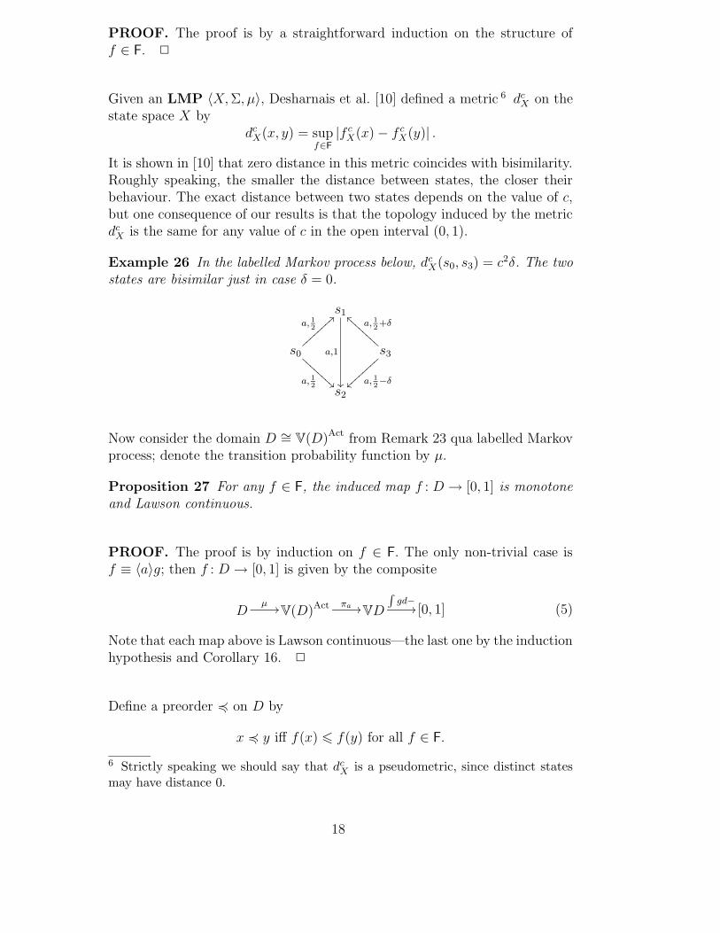
Example 26 In the labelled Markov process below, dcX(s0, s3) = c2δ. The two

states are bisimilar just in case δ = 0.

s1

a,1

��

s0

a, 12

>>||||||||

a, 12

BBBB

BBBB

s3

a, 12+δ

``BBBBBBBB

a, 12−δ~~||

||||

||

s2

Now consider the domain D ∼= V(D)Act from Remark 23 qua labelled Markovprocess; denote the transition probability function by µ.

Proposition 27 For any f ∈ F, the induced map f : D → [0, 1] is monotoneand Lawson continuous.

PROOF. The proof is by induction on f ∈ F. The only non-trivial case isf ≡ 〈a〉g; then f : D → [0, 1] is given by the composite

Dµ

//V(D)Act πa //VD

∫

gd−// [0, 1] (5)

Note that each map above is Lawson continuous—the last one by the inductionhypothesis and Corollary 16. 2

Define a preorder 4 on D by

x 4 y iff f(x) 6 f(y) for all f ∈ F.

6 Strictly speaking we should say that dcX is a pseudometric, since distinct states

may have distance 0.

18

Since each functional expression gets interpreted as a monotone function, x vy implies x 4 y. Theorem 29 asserts that the converse also holds. In order toprove this result we need the following lemma.

Note that in the lemma we distinguish between an upper set V ⊆ D, and a4-upper set U ⊆ D (x ∈ U and x 4 y implies y ∈ U).

Lemma 28 If a ∈ Act, x 4 y and U ⊆ D is Scott open and 4-upper, thenµx,a(U) 6 µy,a(U).

PROOF. Let K = {x1, . . . , xm} ⊆ U and z ∈ D \ U be given. For eachi ∈ {1, . . . ,m}, since xi 64 z, there exists gi ∈ F such that gi(xi) > gi(z). SinceF is closed under truncated subtraction, and each gi is Lawson continuous, wemay, without loss of generality, assume that gi(xi) > 0 and gi is identicallyzero on a Lawson-open neighbourhood of z. Moreover, if we set gz = maxi gi,then gz ∈ F is identically zero in a Lawson-open neighbourhood of z and isbounded away from 0 on ↑K. Such a function gz can be exhibited for anyz ∈ D \ U .

Since D\U is Lawson compact (being Lawson closed) we can pick z1, . . . , zm ∈D \U such that f = minj gzj

is identically zero on D \U and is bounded awayfrom zero on ↑K by, say, r > 0. Finally, setting h = min(f, r), we get

µx,a(↑K) 61

r

∫

hdµx,a 61

r

∫

hdµy,a 6 µy,a(U),

where the middle inequality follows from (〈a〉h)(x) 6 (〈a〉h)(y).

Since U is the (countable) directed union of sets of the form ↑K for finiteK ⊆ U , it follows that µx,a(U) 6 µy,a(U). 2

Theorem 29 The order on D coincides with 4.

PROOF. Let σD denote the Scott topology on D and τ the topology of Scott-open 4-upper sets. Consider the following diagram, where ι is the continuousmap given by ιx = x.

〈D, σD〉

ι

��

µ//V〈D, σD〉

Act

VιAct

��

〈D, τ〉µ′

//______ V〈D, τ〉Act

(6)

Since ι is a bijection there is a unique function µ′ making the above diagramcommute in the category of sets.

19

Recall that the topology on V〈D, τ〉 is generated by sub-basic opens of theform {ν | νU >r} for U ∈ τ and 0<r<1. The inverse image of such a set underµ′ is Scott open by the Scott continuity of µ and is 4-upper by Lemma 28.Thus µ′ is a continuous map and yields a VAct-coalgebra structure on 〈D, τ〉.

The finality of the VAct-coalgebra 〈〈D, σD〉, µ〉, as indicated in Remark 23,implies that ι has a continuous left inverse, and is thus a homeomorphism.Hence, for each y ∈ D, the Scott-closed set ↓ y is τ -closed, and thus 4-lower.Thus x 4 y implies x v y. 2

Corollary 30 (Theorem 4.10[11]) Let 〈X, Σ, µ〉 be a labelled Markov pro-cess with X an analytic space. Denote by v the bisimilarity relation on X.Then x v y iff f c

X(x) = f cX(y) for all functional expressions f ∈ F.

PROOF. Let g denote the unique zig-zag map from 〈X, Σ, µ〉 to the finalLMP, i.e., the domain D from Remark 23. Then

x v y⇔ g(x) = g(y) by Propositions 5 and 8

⇔ f cD(g(x)) = f c

D(g(y)) for all f ∈ F, by Theorem 29

⇔ f cX(x) = f c

X(y) for all f ∈ F, by Proposition 25.

2

Remark 31 Corollary 30 has already appeared as [11, Theorem 4.10]. Theproof there is quite different. Among other things it relies on a modal logiccharacterizing bisimilarity from [9], a translation between functional expres-sions and formulas of the modal logic, and an approximation scheme for re-covering an arbitrary LMP as the join of a chain of finite-state approximants.These last two points are discussed at greater length in Section 9. We shouldadd that [11] also proves that given an LMP 〈X, Σ, µ〉, x ∈ X is simulated byy ∈ X just in case f c

X(x) 6 f cX(y) for all functional expressions f .

Since we view the domain D as a labelled Markov process, we can considerthe metric dc

D as defined in Section 3. We will need the following result.

Proposition 32 (Lemma 4.6[10]) Suppose 0<c<1 and Act is finite. Thengiven ε > 0, there exists finite F′ ⊆ F such that for all x, y ∈ D

0 6 dcD(x, y)− sup

f∈F′

|f cD(x)− f c

D(y)|< ε.

Theorem 33 For 0<c<1 and finite Act the Lawson topology on D is inducedby dc

D.

20

PROOF. The Lawson topology on D is compact. By Theorem 29, dcD is a

metric (not just as pseduometric), and so it induces a Hausdorff topology. Thusit suffices to show that the Lawson topology is finer than the topology inducedby dc

D. Now if xn → x in the Lawson topology, then f(xn) → f(x) for eachf ∈ F, since each functional expression is interpreted as a Lawson-continuousmap. Now, by Proposition 32, dc

D(xn, x)→ 0 as n→∞. 2

Remark 34 Both hypotheses in the above theorem are necessary. In partic-ular it is shown in [10] that the topology induced by dc

X differs for c < 1 andc = 1.

We defined a metric dcX for each labelled Markov process X. However, if one

thinks of a labelled Markov process X = 〈X, Σ, µ〉 as being equipped with adistinguished (initial) state sX , then one can define a metric dc on the classLMP of all labelled Markov processes by

dc(X,Y ) = supf∈F

|f cX(sX)− f c

Y (sY )|.

Corollary 35 For 0 < c < 1 the topology on LMP induced by dc is compactand independent of the value of c.

PROOF. Consider the function LMP → D mapping a labelled Markovprocess X to the image of the distinguished state sX under the unique zig-zagmap X → D. By Proposition 25 this map is an isometry (i.e., a distancepreserving map) 〈LMP , dc〉 → 〈D, dc

D〉. Furthermore this map it is clearlysurjective. The stated results now easily follow from Theorem 33. 2

8 Testing

In this section we characterize similarity on an LMP as a testing preorder, andbisimilarity as a testing equivalence. The testing formalism we use is that setforth by Larsen and Skou [20]. (See also Abramsky [1] and Bloom and Meyer[5] for similar formalisms.) The idea is to specify an interaction between anexperimenter and a process; the way a process responds to the various kindsof tests determines a simple and intuitive behavioural semantics.

A typical intuition is that a process is a black box whose interface to theoutside world includes a button for each action a ∈ Act. The most basickind of test is to try and press one of the buttons: either the button willgo down and the process will make an invisible state change (correspondingto a labelled transition), or the button doesn’t go down (corresponding to arefusal). An important question arises as to which mechanisms are allowed

21

to combine the basic button-pushing experiments. Here, following Larsen andSkou, we suppose that the tester can save and restore the state of the processat any time. Or rather we make the equivalent assumption that the tester canmake multiple copies of the process in order to experiment independently onone copy at a time. The facility of copying or replicating processes is crucialin capturing branching-time equivalences like bisimilarity.

Definition 36 The test language T0 is given by the grammar

t ::= 1 | at | t · t

where a ∈ Act.

The term 1 represents the test that does nothing but successfully terminate.The term at represents the test: press button a, and in case of success proceedwith test t. We usually abbreviate a1 to just a. Finally, t1 · t2 specifies the test:make two copies of (the current state of) the process, perform the test ti onthe i-th copy, and record success in case both sub-tests succeed.

Definition 37 Given a labelled Markov process 〈X, Σ, µ〉, we define an in-dexed family {P (−, t)}t∈T0

of real-valued random variables on 〈X, Σ〉 by

P (x, 1) = 1

P (x, at) =∫

P (−, t)dµx,a

P (x, t1 · t2) = P (x, t1) · P (x, t2)

Intuitively P (x, t) is the probability that state x passes test t.

The following simple example motivates the inclusion of the branching con-struct in T0.

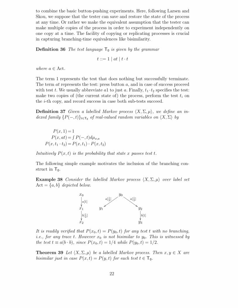
Example 38 Consider the labelled Markov process 〈X, Σ, µ〉 over label setAct = {a, b} depicted below.

x0

a[1]

��

y0a[ 1

2]

zzvvvvvvvvva[ 1

2]

$$IIIIIIIII

x1

b[ 12]

��

y1 y2

b[1]��

x2 y3

It is readily verified that P (x0, t) = P (y0, t) for any test t with no branching,i.e., for any trace t. However x0 is not bisimilar to y0. This is witnessed bythe test t ≡ a(b · b), since P (x0, t) = 1/4 while P (y0, t) = 1/2.

Theorem 39 Let 〈X, Σ, µ〉 be a labelled Markov process. Then x, y ∈ X arebisimilar just in case P (x, t) = P (y, t) for each test t ∈ T0.

22

PROOF. Consider the free real vector space V = {∑

λiti | λi ∈ R, ti ∈ T0}over T0. The binary product map on T0 has a unique extension to a bilinearmap V × V → V . Furthermore, P : X × T0 → R has a unique extension to afunction P : X × V → R that is linear in its second argument.

P (−, v) is a bounded real-valued function on X for each v ∈ V . Furthermore,the pointwise product of P (−, v1) and P (−, v2) is just P (−, v1 · v2). Let Adenote the closure of the family of the functions P (−, v) in the Banach alge-bra of all bounded real-valued functions on X equipped with the supremumnorm. Then A is a closed sub-algebra, i.e., it is closed under sums, scalarmultiplication and (pointwise) products. Now it is well-known that any suchsub-algebra is also closed under (pointwise) binary minima and maxima (seeJohnstone [17]). We recall the argument for the reader’s convenience.

It is enough to show that f ∈ A implies |f | ∈ A since

max(f, g) = 12(f + g) + 1

2|f − g| .

Without loss of generality, since A is closed under scalar multiplication, wemay suppose that −1 6 f 6 1. Let g = 1− f 2; then 0 6 g 6 1, and

|f |=√

f 2 =√

1− g

= 1− 12g − 1

8g2 − · · · − 1·3···(2n−3)

2nn!gn − · · ·

But this sum converges uniformly; thus |f | ∈ A, and A is closed under point-wise binary minima and maxima.

Furthermore, given a ∈ Act and v =∑

λiti ∈ V , let v′ =∑

λi ati. Then, bylinearity of the integral, the function x 7→

∫

P (−, v)dµx,a is just P (−, v′). ThusA contains the interpretations of all functional expressions f ∈ F.

Now suppose x, y ∈ X are such that P (x, t) = P (y, t) for all t ∈ T0. ThenP (x, v) = P (y, v) for all all v ∈ V . Thus f(x) = f(y) for all functionalexpressions f ∈ F, and x and y are bisimilar by Corollary 30. 2

Theorem 39 generalizes and simplifies a result of Larsen and Skou [20, The-orem 6.5]. The generalization is that Larsen and Skou’s result only appliedto discrete probabilistic transition systems satisfying the minimal deviationassumption. This last condition says that there is a fixed ε > 0 such that anytransition probability µx,a({y}) is an integer multiple of ε. Theorem 39 sim-plifies [20, Theorem 6.5] in that the test language T0 contains no negativeobservations or failures. We explain this point in more detail in Appendix A.

Given the fact that bisimilarity on an LMP is just mutual similarity, one might

23

conjecture that x ∈ X is simulated by y ∈ X just in case P (x, t) 6 P (y, t) forall t ∈ T0. However the following example shows that this is not the case.

Example 40 Consider the process from Example 38. It is readily verified thatP (x0, t) 6 P (y0, t) for all t ∈ T0. However x0 is not simulated by y0. Inparticular, x1 is only simulated by y2, but the probability of moving from x0 tox1 is greater than the probability of moving from y0 to y2.

There is no hope of using the elements of V to characterize similarity, since Vcontains negative scalar multiples of tests—so the functions P (−, v) are notmonotone with respect to the similarity preorder. On the other hand, if we wereto restrict attention to the cone V+ of positive linear combinations of elementsof T0, then in the example above we would still have P (x0, v) 6 P (y0, v) forall v ∈ V+. Nevertheless the solution we outline below does follow the generalidea of using a ‘monotone’ subset of V as a test language.

One can think of the test t ≡ t1 · t2 as a conjunction, in that t succeeds ifeach of its components succeeds. In order to capture similarity the idea is toconsider more general truth-functional ways of combining tests.

Definition 41 For each n ∈ N, the set Fma(n) of propositional formulas onvariables p1, . . . , pn is generated by the syntax

ϕ ::= > | pi | ϕ ∨ ϕ | ϕ ∧ ϕ .

Under the standard Boolean semantics, each ϕ ∈ Fma(n) is interpreted as afunction ϕB : Bn → B, where B = {false, true}. We also consider a real-valuedsemantics where ϕ ∈ Fma(n) is interpreted as a function ϕR : [0, 1]n → [0, 1].Given r1, . . . , rn ∈ [0, 1], consider n independently distributed Booelan-valuedBernoulli random variables X1, . . . , Xn, where Xi takes value true with prob-ability ri. We define

ϕR(r1, . . . , rn) = P (ϕB(X1, . . . , Xn) = true).

Definition 42 The test language T1 is given by the grammar

t ::= at | ϕ(t1, . . . , tn) [ϕ ∈ Fma(n)] .

Given a labelled Markov process 〈X, Σ, µ〉 and x ∈ X, we extend the definitionof the function P (x,−) from T0 to T1 by

P (x, ϕ(t1, . . . , tn)) = ϕR(P (x, t1), . . . , P (x, tn)) .

A test t ∈ T1 can be viewed as a tree whose edges are labelled with elementsof Act and such that an n-way branching node is labelled by an element of

24

Fma(n). Intuitively, the test t ≡ ϕ(t1, . . . , tn) is implemented as follows. Maken copies of the current state of the process; run test ti on the i-th copy;record success for t if ϕ is true under the (Boolean) valuation v ∈ Bn given byvi = true iff ti succeeds.

If ϕ ≡ p1 ∨ p2, we abbreviate ϕ(t1, t2) to t1 ∨ t2. This test succeeds iff eitherof the disjuncts succeeds. The notation t1 ∧ t2 is interpreted similarly. Bothnotations should be employed with care since neither of these operations isidempotent. In fact, t1 ∧ t2 exactly corresponds to the test t1 · t2 from thelanguage T0.

Theorem 43 Let 〈X, Σ, µ〉 be a labelled Markov process. Then x ∈ X is sim-ulated by y ∈ X iff P (x, t) 6 P (y, t) for all tests t ∈ T1.

Example 44 Recall the process from Example 38 and consider the test t ≡a(b ∨ b). Then P (x0, t) = 3/4 while P (y0, t) = 1/2. Thus t witnesses the factthat x0 is not simulated by y0.

The rest of this section is devoted to a proof of Theorem 43. This proof, whichis inspired by [20, Theorem 6.5], has a statistical flavour and is strikinglydifferent from that of Theorem 39. However, we believe that an alternativeproof using the technology of compact pospaces may be possible (see [17]).

Definition 45 Let 〈X, Σ, µ〉 be a labelled Markov process. Recall that eachfunctional expression f ∈ F defines a function X → [0, 1] (again, take c = 1).Given f ∈ F, 0 6 α < β 6 1 and ε > 0, we say that t ∈ T1 is a test for(f, α, β, ε) if for all x ∈ X,

Whenever f(x) > β then P (x, t) > 1− ε;Whenever f(x) 6 α then P (x, t) 6 ε.

Thus, if test t succeeds on state x, then with high confidence we can assert thatf(x) > α. On the other hand, if t fails on state x, then with high confidencewe can assert that f(x) < β.

Lemma 46 Let 〈X, Σ, µ〉 be a labelled Markov process. Then for any f ∈ F,0 6 α < β 6 1 and ε > 0, there is a test t for (f, α, β, ε).

PROOF. The proof proceeds by induction on f ∈ F. The cases f ≡ 1 andf ≡ g � q are straightforward and we omit them.

Case f ≡ min(f1, f2): By induction, let ti be a test for (fi, α, β, ε/2) for i = 1, 2.

25

Then we take t ≡ t1 ∧ t2 as a test for (f, α, β, ε). Now

min(f1, f2)(x) > β ⇒ f1(x) > β and f2(x) > β

⇒ P (x, t1) > 1− ε/2 and P (x, t2) > 1− ε/2

⇒ P (x, t) > 1− ε,

and

min(f1, f2)(x) 6 α⇒ f1(x) 6 α or f2(x) 6 α

⇒ P (x, t1) 6 ε/2 or P (x, t2) 6 ε/2

⇒ P (x, t) 6 ε/2.

Case f ≡ max(f1, f2): Let ti be a test for (fi, α, β, ε/2) for i = 1, 2. Then wetake t ≡ t1 ∨ t2 as a test for (f, α, β, ε). The justification is similar to the caseabove.

Case f ≡ 〈a〉g: Pick n ∈ N and ε′ > 0. By the induction hypothesis, for1 6 i 6 n we have a test ti for (g, i−1

n, i

n, ε′). Pick ϕ ∈ Fma(n) such that

ϕB(p1, . . . , pn) = true iff 1n|{i | pi = true}| > β+α

2.

The rest of the proof is a calculation to show that for suitably large n andsmall ε′, t ≡ ϕ(at1, . . . , atn) can be used as a test for (f, α, β, ε).

Fix x ∈ X. Let θ1, . . . , θn be independent {0, 1}-valued Bernoulli randomvariables, where θi = 1 with probability P (x, ati). Furthermore, define θ =(1/n)

∑ni=1 θi. Thus P (x, t) = P (θ >

β+α

2).

The induction hypothesis is that for 1 6 i 6 n

g(y) > in⇒ P (y, ti) > 1− ε′ (7)

g(y) 6 i−1n⇒ P (y, ti) 6 ε′ . (8)

We estimate P (x, ati) by conditioning on the value of g using (7) and (8).

(1− ε′)µx,a

{

g >i

n

}

6 P (x, ati) 6 µx,a

{

g >i− 1

n

}

+ ε′.

Since E[θ] = 1n

∑ni=1 P (x, ati), it follows that

(1− ε′)

n

n∑

i=1

µx,a

{

g >i

n

}

6 E[θ] 61

n

n∑

i=1

µx,a

{

g >i− 1

n

}

+ ε′.

26

Whence, by a straightforward manipulation of terms in the summation,

(1− ε′)n

∑

i=1

i

nµx,a

{

i

n6 g <

i + 1

n

}

6 E[θ] 6

n∑

i=1

i

nµx,a

{

i− 1

n< g 6

i

n

}

+ ε′

Thus we can choose ε′ small enough and n large enough to ensure that

|E[θ]−∫

gdµx,a|<β−α

4. (9)

Since V [θ] = (1/n2)∑n

i=1 V [θi] 6 1/n, by Chebyshev’s inequality [14] for largen it holds that

P{

|θ − E[θ]| 6 β−α

4

}

> 1− ε. (10)

It is straightforward that the choice of ε′ and n required to make (9) and (10)true can be made independently of x ∈ X. Now

(〈a〉g)(x) > β ⇒∫

gdµx,a > β by definition of 〈a〉g

⇒ E[θ] >3β+α

4by (9)

⇒ P(

θ >β+α

2

)

> 1− ε by (10)

⇒ P (x, t) > 1− ε.

Similarly it follows that (〈a〉g)(x) 6 α⇒ P (x, t) 6 ε. 2

Theorem 43 now follows from Lemma 46 using the characterization of simu-lation in terms of functional expressions from Remark 31.

9 Conclusion and Related Work

The theme of this paper has been the use of domain-theoretic and coalgebraictechniques to analyze labelled Markov processes. These systems generalize thediscrete labelled probabilistic processes investigated by Larsen and Skou [20].Our main results extend and simplify the work of Larsen and Skou on theconnection between probabilistic bisimulation and testing. The direction ofthis generalization, and the ideas and techniques we use, are mainly inspired bythe work of Desharnais, Edalat, Gupta, Jagadeesan and Panandagen [9,10,12].In particular, as we now explain, there are several interesting parallels betweenthe results reported here and their work on the logical characterization ofbisimilarity.

A central result of Larsen and Skou [20] was a logical characterization ofbisimilarity for discrete LMPs satisfying the minimum deviation assumption.

27

The formulas in their logic were generated by the grammar

ϕ ::= > | ϕ ∧ ϕ | ϕ ∨ ϕ | 〈a〉qϕ | ∆a (11)

where a ∈ Act and q ∈ [0, 1] ∩Q.

This is a probabilistic version of Henessey-Milner logic [21]. The semantics isgiven by a satisfaction relation � between states of a labelled Markov processand formulas. In particular, one has x � 〈a〉qϕ if the probability that x makesan a-labelled transition to the set of states satisfying ϕ exceeds q. Also x �

∆a just in case no a-transition is possible from x. This logic characterizesbisimilarity in the sense that states satisfy the same formulas just in case theyare bisimilar.

In generalizing the result of Larsen and Skou beyond the discrete case, Deshar-nais et al. [9] realized that an even simpler logic, generated by the grammar

ϕ ::= > | ϕ ∧ ϕ | 〈a〉qϕ , (12)

is sufficient to characterize bisimilarity for all LMPs. This is reflected in ourobservation that negative observations, or failures, are not needed to test forbisimilarity. Indeed the grammar for the smaller logic is very similar in formto the grammar for tests in Definition 36. The one significant difference isthat in the grammar for tests the modalities are not indexed with numbers.Of course, the semantics of tests is completely different, with, in particular,an arithmetic interpretation of conjunction as multiplication.

It was later shown in [12] that the logic (12) is inadequate to characterizesimilarity: one needs to include disjunction. Again, this is reminiscent of theobservation that the test language in Definition 36 doesn’t characterize sim-ilarity, and that one needs to use the more general test language T1 fromDefinition 42.

We would also like to clarify the relationship between parts of this work andthe paper [12] on approximating LMPs. That work features the same domainequation D ∼= V(D)Act appearing in the present paper; furthermore, the au-thors exhibit a two-stage construction for interpreting an arbitrary LMP inD. In the first stage they show how to interpret a finite-state LMP as an ele-ment of D. The second stage utilizes a method for unfolding and discretizingan arbitrary LMP X = 〈X, Σ, µ〉 into finite-state approximants. In fact theyproduce a sequence of finite approximants, which is a chain in the simulationorder, and such that any formula satisfied by X is also satisfied by one of thefinite approximants. Then they define the interpretation of X in the domain Dto be the join of the interpretations of its finite approximants. Using their re-sults on the logical characterization of bisimilarity they show that each LMPis bisimilar to its interpretation in D. It follows that their domain-theoretic

28

semantics is the same as our final semantics.

As far as we are aware, it was de Vink and Rutten [24] who were the first tostudy probabilistic transition systems as coalgebras. However, since they workwith ultrametric spaces, their results only apply in the discrete setting, notto arbitrary LMPs. It was also noted in [9] that LMPs are coalgebras of theGiry functor, although this observation was not developed there.

An interesting problem, suggested by the development in Section 8, wouldbe to realize the final LMP as the Gelfand-Naimark dual of an equationallypresented C∗-algebra. The idea would be to take the free vector space V inSection 8 and quotient by a suitable set of equations to get a commutativealgebra. An issue that is as yet unresolved is how to define a suitable norm inorder to get a C∗-algebra. We conjecture that this can be done, and moreoverthat the final LMP can be recovered as the space of characters of the resultingalgebra.

Acknowledgements

We thank the anonymous referees for numerous suggestions for improving thepresentation of the paper. In particular, their comments helped us find a moretransparent formulation of the testing results in Section 8.

References

[1] S. Abramsky. Observation equivalence as a testing equivalence. TheoreticalComputer Science, 53:225–241, 1987.

[2] J. Adamek and V. Koubek. On the greatest fixed point of a set functor,Theoretical Computer Science, 150:57–75, 1995

[3] M. Alvarez-Manilla, A. Edalat, and N. Saheb-Djahromi. An extension result forcontinuous valuations. Journal of the London Mathematical Society, 61(2):629–640, 2000.

[4] W. Averson. An Invitation to C*-Algebras. Springer-Verlag, 1976.

[5] B. Bloom and A. Meyer. Experimenting with process equivalence. TheoreticalComputer Science, 101:223-237, 1992.

[6] F. van Breugel and J. Worrell. An Algorithm for Quantitative Verification ofProbabilistic Transition Systems. In Proc. 12th International Conference onConcurrency Theory, volume 2154 of LNCS, Springer-Verlag, 2001.

29

[7] F. van Breugel, S. Shalit and J. Worrell. Testing Labelled MarkovProcesses. In Proc. 29th International Colloquium on Automata, Languages andProgramming, volume 2380 of LNCS, Springer-Verlag 2002.

[8] F. van Breugel, M. Mislove, J. Ouaknine and J. Worrell. AnIntrinsic Characterization of Approximate Probabilistic Bisimilarity. In Proc.Foundations of Software Science and Computation Structures (FOSSACS 03),volume 2620 of LNCS, Springer-Verlag, 2003.

[9] J. Desharnais, A. Edalat and P. Panangaden. Bisimulation for Labelled MarkovProcesses. Information and Computation, 179(2):163–193, 2002.

[10] J. Desharnais, V. Gupta, R. Jagadeesan, and P. Panangaden. Metricsfor Labeled Markov Processes. In Proc. 10th International Conference onConcurrency Theory, volume 1664 of LNCS, Springer-Verlag, 1999.

[11] J. Desharnais, V. Gupta, R. Jagadeesan, and P. Panangaden. Metrics forLabeled Markov Systems. Accepted to Theoretical Computer Science, 2004.

[12] J. Desharnais, V. Gupta, R. Jagadeesan, and P. Panangaden. ApproximatingLabeled Markov Processes. Information and Computation, 184(1):160–200,2003.

[13] A. Edalat. When Scott is weak at the top. Mathematical Structures in ComputerScience, 7:401–417, 1997.

[14] G.A. Edgar. Integral, Probability, and Fractal Measures. Springer-Verlag, 1998.

[15] G. Gierz, K. Hofmann, K. Keimel, J. Lawson, M. Mislove, D. Scott. ContinuousLattices and Domains, Cambridge, 2003.

[16] M. Giry. A Categorical Approach to Probability Theory. In Proc. InternationalConference on Categorical Aspects of Topology and Analysis, volume 915 ofLecture Notes in Mathematics, Springer-Verlag, 1981.

[17] P. Johnstone. Stone Spaces. Cambridge University Press, 1982.

[18] C. Jones. Probabilistic nondeterminism, PhD Thesis, Univ. of Edinburgh, 1990.

[19] A. Jung and R. Tix. The Troublesome Probabilistic Powerdomain. In ThirdWorkshop on Computation and Approximation, Proceedings. Electronic Notesin Theoretical Computer Science, vol 13, 1998.

[20] K.G. Larsen and A. Skou. Bisimulation through Probabilistic Testing.Information and Computation, 94(1):1–28, 1991.

[21] R. Milner. Communication and Concurrency. Prentice Hall, 1989.

[22] K.R. Parthasarathy. Probability Measures on Metric Spaces. Academic Press,1967.

[23] M. Smyth and G. Plotkin. The Category Theoretic Solution of RecursiveDomain Equations, SIAM Journal of Computing, 11(4):761–783, 1982.

30

[24] E.P. de Vink and J.J.M.M. Rutten. Bisimulation for Probabilistic TransitionSystems: a Coalgebraic Approach. Theoretical Computer Science, 221(1/2):271-293, June 1999.

A Tests and Observations

Below we recall the testing formalism used by Larsen and Skou [20] to charac-terize probabilistic bisimilarity on discrete systems. This framework was alsoused in an earlier version of this paper [8]. We show that the test languagesT0 and T1, introduced in Definitions 36 and 42 respectively, correspond to twofragments of Larsen and Skou’s language.

In fact, the set TLS of tests introduced by Larsen and Skou is almost exactlythe same as T0. The only difference in the syntax is that in TLS tupling playsthe role of multiplication. However, rather than considering only that a testmay succeed or fail, Larsen and Skou associate to each test t ∈ TLS a set Ot

of observations. In this way they account for the fact that some branches of tmay succeed while others may fail.

Definition 47 ([20]) The test language TLS is given by the grammar

t ::= 1 | at | 〈t1, . . . , tn〉

where a ∈ Act.

For t ∈ TLS the set of observations Ot is defined by

O1 = {1}

Oat = {a×} ∪ {ae | e ∈ Ot}

O〈t1,...,tn〉 = Ot1 × · · · ×Otn .

The only observation of the test 1 is success—which is again denoted 1. Anobservation of at is either failure of a, denoted a×, or success of a followedby observation e ∈ Ot, denoted ae. An observation of a tuple test 〈t1, . . . , tn〉consists of a tuple 〈e1, . . . , en〉, where ei is an observation of ti.

Thus Ot is a set of mutually exclusive and exhaustive observations that mightarise when test t is performed. Given an LMP 〈X, Σ, µ〉, each state x ∈ Xinduces a probability distribution Pt(x,−) on Ot according to the followingrules.

31

P1(x, 1) = 1

Pat(x, ae) =∫

Pt(−, e)dµx,a

Pat(x, a×) = 1− µx,a(X)

P〈t1,...,tn〉(x, 〈e1, . . . , en〉) = Pt1(x, e1) · · ·Ptn(x, en)

Thus Pt(x, e) is the probability of making observation e when test t is run instate x. Given E ⊆ Ot we write Pt(x,E) =

∑

e∈E Pt(x, e), i.e., the probabilityof observing some result in E. Larsen and Skou [20, Theorem 6.5] showed thatin a discrete LMP satisfying the minimal deviation assumption, two states xand y are bisimilar just in case Pt(x,E) = Pt(y, E) for all tests t ∈ TLS andE ⊆ Ot.

Next we show how to intepret the language T1 in TLS.

Proposition 48 For each test t ∈ T1 there is a test t′ ∈ TLS and a set ofobservations E ⊆ Ot′ such that, for any LMP 〈X, Σ, µ〉 and x ∈ X, P (x, t) =Pt′(x,E).

PROOF. The proof is by induction on t ∈ T1. The base case> ∈ T1 is trivial.Consider now the test at. By induction there exists t′ ∈ TLS and E ⊆ Ot′ suchthat P (x, t) = Pt′(x,E) for all x ∈ X. Then, by linearity of the integral, weget that P (x, at) = Pat′(x, aE) for all x ∈ X, where aE = {ae | e ∈ E}.Finally, suppose t ≡ ϕ(t1, . . . , tn), and, by induction, let t′i ∈ TLS and Ei ⊆ Ot′

i

be such that P (x, ti) = Pt′i(x,Ei) for all x ∈ X. Write t′ ≡ 〈t′1, . . . , t

′n〉 and

define E ⊆ Ot′ by

E = {〈e1, . . . , en〉 | ϕB(e1 ∈ E1, . . . , en ∈ En) = true} .

When test t′i is run in state x, the probability of making an observation in Ei

is Pt′i(x,Ei). We conclude that Pt′(x,E) = ϕR(Pt′

1(x,E1), . . . , Pt′n

(x,En)) (cf.Definition 41). Now

P (x, t) = ϕR(P (x, t1), . . . , P (x, tn))

= ϕR(Pt′1(x,E1), . . . , Pt′n

(x,En))

= Pt′(x,E) .

Example 49 Corresponding to the test a(b∨ b) in T1 is the test a〈b, b〉 in TLS

with set of observations E = {a〈b, b〉, a〈b×, b〉, a〈b, b×〉}.

Remark 50 Given a test t ∈ T0, the corresponding test t′ ∈ TLS is obtainedby a trivial syntactic replacement of multiplication by tupling. Futhermore theassociated set of observations E ⊆ Ot′ is just the singleton {t′}, i.e., theobservation that all parts of the test succeed.

32