domestic violence, bargaining and fertility in rural … violence, bargaining and fertility in rural...
TRANSCRIPT
Domestic Violence, Bargaining and Fertility in Rural Tanzania
Melissa González-Brenes
Department of Economics
University of California, Berkeley
DRAFT
November 30, 2003
Abstract: This paper uses an original dataset from rural Tanzania to explore both the
determinants of domestic violence and the relationship of violence with other welfare outcomes
for household members. A quarter of all women report being victims of domestic violence, half
of these women report being victims of violence in the previous year. Preliminary results suggest
that women are more vulnerable during childbearing years, and that relationships to female
relatives play an important part in reducing violence. I find no relationship between violence and
measures of household wealth.
2
1 Introduction
In rural Tanzania, domestic violence against women is widespread. Existing laws (e.g.,
Marriage Act of 1971) prohibit corporal punishment by husbands, and grant spouses equal rights
to matrimonial property acquired through joint effort. In practice, however, women are often
denied these rights. Community leaders regard beating as an acceptable punishment that
husbands inflict on their wives (Wandel et al., 1991).
This paper uses an original dataset from rural Tanzania to explore both the determinants
of domestic violence and the relationship of violence with other welfare outcomes for household
members. In contrast with most existing empirical work, the analysis is based on a sample of
representative households. Prevalence is high: a quarter of all women report being beaten by
their husbands at some point in the past, half of whom report being beaten in the last year. The
dataset collected includes information at the individual, couple, household and community level.
In economics, domestic violence is often cited in the context of intra-household
bargaining as one reason it may not be appropriate to assume a cooperative bargaining process of
household decision-making for all households. An examination of the differences between
violent and non-violent households can shed light on the relationship between violence and
bargaining.
Empirical work in intra-household bargaining has typically included capital investments,
including human capital, as explanatory variables. However, social capital may also play a role
in household decision-making. Moreover, if the types of capital that have been traditionally
included in the empirical estimation of intra-household allocation models are restricted for
women in a particular setting, then the exclusion of certain types of capital or investments is not
gender neutral. A rich dataset that includes formal and informal measures of social capital at the
individual, household and community level allows me to explore the relationship between social
networks and the prevalence of domestic violence.
2 Related literature
A subset of the economic literature on household decision-making has attempted to
model domestic violence. The theoretical models of domestic violence are modifications of
existing bargaining models. Tauchen, Witte and Long (1991) present a non-cooperative
bargaining model in which violence serves both an expressive and an instrumental purpose: it
enters the husband’s utility directly as well as indirectly through his wife’s behavior. In this

3
model, men “purchase” violence from women with income transfers, so that the level of resources
controlled by each partner and whether the reservation utility constraint is binding determine the
level of violence in equilibrium. Farmer and Thiefenthaler (1997) also model the determinants of
violence in the context of a non-cooperative game. The comparative statics from the model
predict that women’s income and other financial support received from outside the marriage
changes the woman’s threat point and thus decreases the level of violence. This is done by
including a catch-all term for resources outside the marriage--including but not limited to welfare
payments, divorce settlements, and other support services--that enters the woman’s reservation
utility additively.
Farmer and Thiefenthaler (1996) attempt to explain the large numbers of women who
return to an abusive relationship after seeking help. Many battered women may use shelters and
other support services for battered women as a signal to the batterer, something that can change
their threat-point. This idea is formalized as a non-cooperative game.
More recently, a paper by Robert Pollak (2002) attempts to explain the prevalence of
domestic violence –as opposed to its causes—by modeling the inter-generational transmission of
domestic violence. The model incorporates the stylized facts of family violence: children who
grow up in violent households are more likely to live in violent households as adults—either as
batterers or victims. In addition, the model incorporates the role of marital formation and
dissolution in the prevalence of violence by assuming that individuals who grew up in violent
homes are more likely to marry partners who grew up in violent homes. In this model, assortative
mating increases the equilibrium level of violence.
Empirical work on the causes of violence in economics is limited; most existing studies
are based on nonrandom samples of battered women. An exception to this is work by Bloch and
Rao (2000), who use a representative sample of women from three rural villages in India to
examine the relationship between dowries and violence. They argue that violence is used as a
bargaining instrument to extract larger dowry payments from the bride’s family.
Tauchen et al. (1991) include empirical work based on a sample of 125 women referred
from shelters and other advocates for battered women. They find that the effect of income on
violence depends on the income level of the couple. For low and middle income couples in their
sample, an increase in the man’s income is positively associated with violence, and the reverse is
true for changes in female income. The effect of income for higher-income couples in the sample
depends on the identity of the main income earner. For households in which the man is the main
earner, an increase in income is associated with a decrease in violence, regardless of the identity
of the income recipient. In contrast, households in which the woman is the main earner, increases

4
in her income are associated with increased violence. In addition, male employment, but not
female employment, is negatively and significantly related to violence. For non-economic
variables, violence is positively related to the age difference, and negatively related to male age.
There is no difference in frequency of violence for different ethnic groups.
Tauchen and Witte (1995) use data from an experiment carried out by the Minneapolis
Police Department to examine how police treatment in cases of domestic violence affects
subsequent violence. The experiment was designed to learn how the police could best handle
domestic violence calls. Each police officer was responding to an incidence of misdemeanor
domestic violence in which a woman had been assaulted by her male romantic partner. The
officer was randomly “assigned” an intervention strategy: (i) advising the couple, (ii) separating
the individuals temporarily, or (iii) arresting the suspect. The data collected from interviews with
the women includes age, education, and employment status for men and women, as well as the
assailant’s arrest history. They find that in the very short-term, arrest is the most effective
deterrent against future violence. However, there is no difference between the three interventions
by the end of the six months (that is, arrest is most effective at deterring violence temporarily).
Lagged violence is the most important predictor of violence in the current period. Interestingly,
the only individual characteristic significantly related to violence is the man’s current
employment status, but not employment history.
There is a rich literature on the causes of domestic violence in other social sciences,
particularly sociology and psychology. Sociological models link violence to gender inequality.
The causes of violence lie in the way society is organized: unequal economic opportunities
available to women and men, the protection—or lack thereof—offered to victims by the legal
system, and (un)availability of other institutional resources for victims are among the
determinants of violence (Pagelow, 1981). Quantitative studies of the determinants of violence in
developed countries consistently find a positive correlation between violence against women,
traditional notions of men and women’s role in the household, and male unemployment.
In contrast, psychological models focus on individual characteristics as determinants of
violence. In terms of the batterer, violence is linked to low self-esteem, pathological jealousy,
and severe stress. The psychological literature on domestic violence places emphasis on the link
between violence and the batterer’s desire for control over the victim. Violence often goes hand
in hand with a curtailment of the victim’s economic and social independence (Walker, 1984).
The anthropological and sociological literature on the societal determinants of violence
includes comparative work that focuses on domestic violence (the term used in this literature is
wife-beating, to make explicit the fact that what is being studied is violence perpetrated by men

5
on women in the context of a permanent relationship, see Counts et al.). Among these
comparative or cross-country studies is work by Levinson (1989), who uses data from ninety
societies to examine the relationship between the prevalence of domestic violence and economic
and legal institutions. He finds that the prevalence of wife beating is higher in places where men
control family wealth, conflicts are solved by means of physical violence, and women do not
have an equal right to divorce. In addition, there is less incidence of wife beating in societies
characterized by female work groups.
3 Setting: Meatu District
Meatu is a semi-arid rural district in Western Tanzania. It is poor even by Tanzanian
standards, with income per capita in 2001 at USD$184, roughly two-thirds of the World Bank
estimate for Tanzania as a whole. About two-thirds of this consumption-based measure of
income consists of food produced and consumed at home. The main ethnic group is the Sukuma,
which comprise 90 percent of the population. About half of all households report owning some
cattle, and 60 percent cultivate cotton, the main cash crop.
The District is divided into three Divisions: Kimali, Kisesa and Nyalanja, and 71 villages.
There are large differences between administrative divisions within the District. Of the three
Divisions—Kimali, Kisesa, and Nyalanja—households in Nyalanja are larger, poorer, and less
educated. There are also differences in ethnic composition and soil aridity within the District,
which result in different cropping patterns.
5 Data and Estimation Methods
5.1 Data Set
The data used comes from surveys administered in Meatu District, Tanzania, in 2001 and
2002. The analysis is based primarily on two surveys conducted from June thru August 2002.
During this period, a survey of 1,200 representative households was carried out throughout the
District. The 2002 Household Survey includes data on household composition, demographics,
asset ownership, savings patterns, economic activities and social capital. A separate survey
instrument, the Meatu Family Survey, was administered to a subset of women in 280 of the
households surveyed. This survey includes information on marriage and fertility history, marital
quality, household decision-making, and conflict resolution between spouses, including the
prevalence of domestic violence. Community-level data comes from the 2001 and 2002 Village
Council Survey, in which community leaders were asked about village history, traditions around
marriage and divorce, and composition of the Village Council, among other things. I was
involved in all stages of the data collection process, from survey design and pre-testing to survey
administration. Table 1 presents sample descriptive statistics.
6
Research on domestic violence is limited in part due to the sensitive nature of the subject.
The Family Survey was administered in a way in which women would feel safe answering all
questions. Enumerators were sent in male-female pairs. In the case that both the husband and wife
were at home at the time of the survey, the male enumerator conducted the household survey with
the husband while the female enumerator interviewed the wife, after receiving permission from
the husband. The protocol was identical if the household survey was administered to someone
other than the husband of the Family Survey respondent. The male enumerator was instructed to
move to a separate location with the Household Survey respondent, while the female enumerator
remained with the Family Survey respondent in her place of work (women who were at home
were often involved in the preparation of food).
Three pairs of female and male enumerators administered the Household and Family
Surveys. There are no systematic differences in reporting rates by enumerator. All three female
enumerators conducting the Family Survey are local residents of Meatu District, and fluent in
Swahili and Kisukuma, the vernacular of the main ethnic group in the District. Household
surveys were conducted in Swahili. Family Survey respondents were given the option to answer
the survey in Swahili or Kisukuma, and often opted for the latter. Swahili is widespread –it is the
language of instruction in primary school and the language of business and politics. In that sense,
it is associated with masculine spheres of action and influence. Many women have little or no
education and feel more comfortable discussing these issues in Kisukuma. In addition, it is often
the language spoken at home by both men and women.
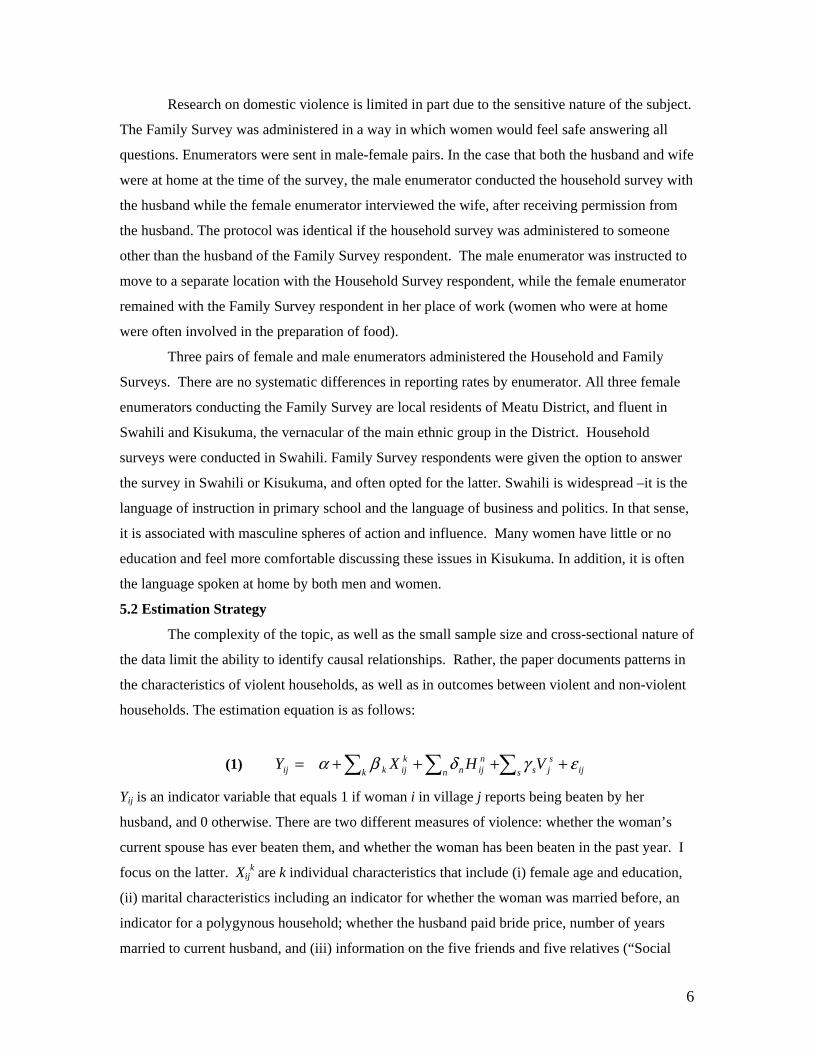
5.2 Estimation Strategy
The complexity of the topic, as well as the small sample size and cross-sectional nature of
the data limit the ability to identify causal relationships. Rather, the paper documents patterns in
the characteristics of violent households, as well as in outcomes between violent and non-violent
households. The estimation equation is as follows:
(1) ∑∑∑ ++++=s ij
sjsn
nijn
kijk kij VHXY εγδβα
Yij is an indicator variable that equals 1 if woman i in village j reports being beaten by her
husband, and 0 otherwise. There are two different measures of violence: whether the woman’s
current spouse has ever beaten them, and whether the woman has been beaten in the past year. I
focus on the latter. Xijk are k individual characteristics that include (i) female age and education,
(ii) marital characteristics including an indicator for whether the woman was married before, an
indicator for a polygynous household; whether the husband paid bride price, number of years
married to current husband, and (iii) information on the five friends and five relatives (“Social

7
networks”) with whom the woman speaks most frequently. Hijn are n household characteristics
including household size, indicators for iron roof and cattle ownership as income proxies, and
household community group membership by gender. Vjs are village characteristics, including the
number of women on the Village Council (a group of local elected officials) and local density of
community groups. The error term, εij is assumed to be independent across households but
clustered within villages.
The current specifications include indicators for iron roof and cattle ownership as income
proxies. However, the survey includes detailed information on household asset ownership that
could be used to create a continuous measure of wealth. The data also includes information on the
identity of the household member that owns the asset (including a code for family ownership).
However, there is little variation in the intra-household ownership of assets by gender. With few
exceptions, women own their clothes and kitchen implements, while men own all other assets.
6 Preliminary Empirical Results
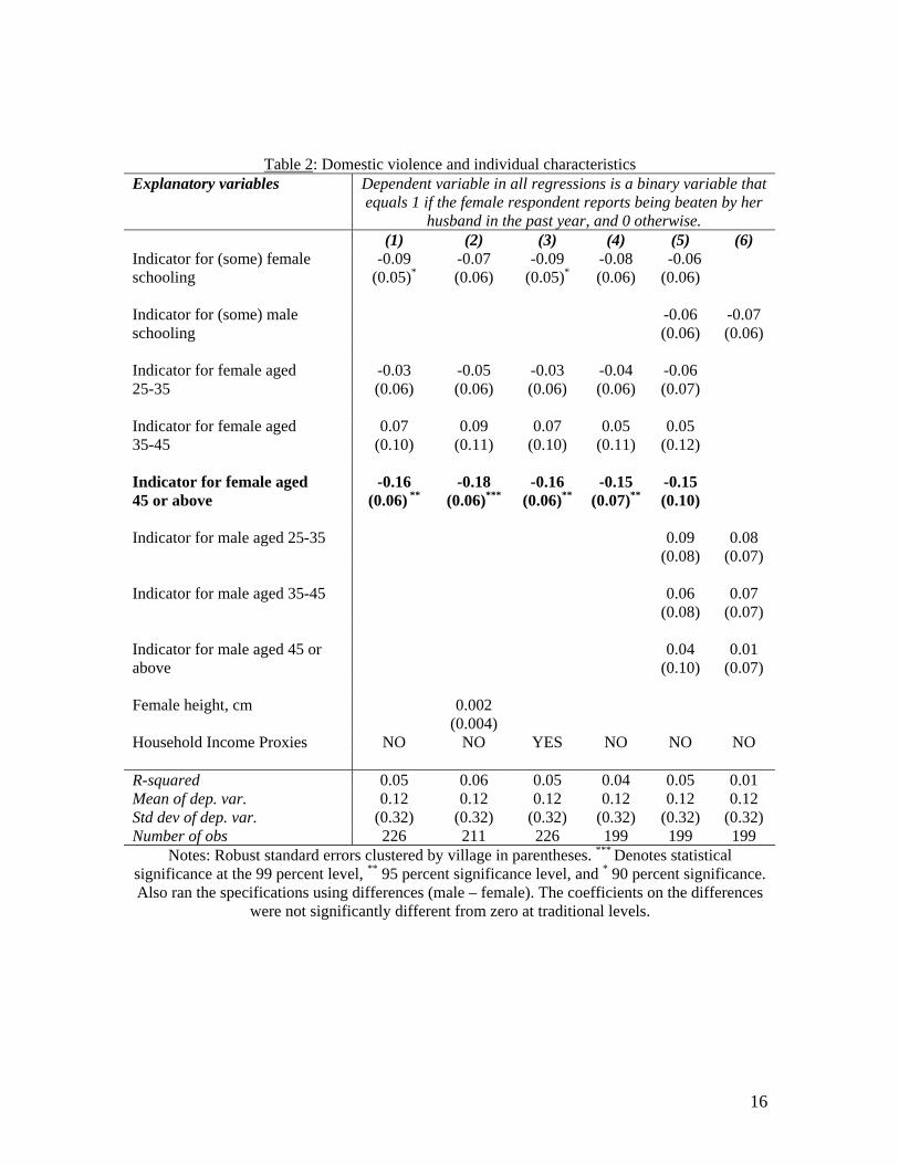
6.1 Individual characteristics and violence
The main result is that violence decreases with female age. The result is driven by a
decrease in violence for women over 45 years of age, who have completed their fertility. Table 2
presents results for the linear probability model; the coefficients should be interpreted as
probabilities. The omitted age category is for women 16 to 25 years old. Prevalence for women
between 25 and 45 years old are no different than those for younger women: the estimated age
coefficients on these categories are not significantly different from zero. Women over 45 years
old are 16 percent less likely than younger women (16-25) to be victims of violence. The
magnitude and significance of the coefficient is consistent across specifications and robust to the
inclusion of marriage and household characteristics.
There is no relationship between male age and the prevalence of violence. Specification (4)
in Table 2 includes male as well as female characteristics, while (4) includes only male
characteristics. In general, information on men is more likely to be missing than female data. In
general, I estimate the models excluding male characteristics in order to use a larger sample.
However, the results presented are robust to the inclusion of male age and education. The
coefficients on male age categories are not significantly different from zero if female
characteristics are excluded.
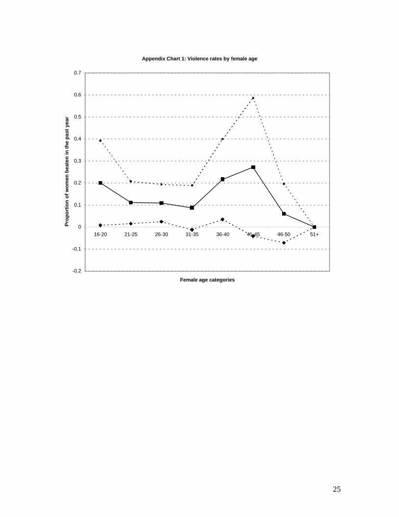
Violence does not decrease steadily with female age, it occurs at the end of women’s
childbearing years. Women in rural Tanzania often marry at the end of their teenage years and
start having children soon afterwards. Appendix chart 1 presents violence prevalence rates by
five-year female age categories. If anything, violence seems to increase between the early 20s

8
and the late 30’s, and starts to decrease for women 40-45 years old. Only one woman over 45
years of age reported being beaten by her husband in the last year. Of course, the small sample
sizes for each age category—reflected in the large standard errors also shown—make it
impossible to distinguish statistically between the prevalence rates for women under 45 years old,
or to make a strong argument for a discontinuity around 45 years of age.
In Tanzania, parenthood confers status to both men and women. However, for women
parenthood is not only an honor but also an obligation. It is defined as a duty of wives to provide
children to their husbands. For a majority of women in this sample (84 percent), it is also a
contractual obligation established at the time of marriage.
Marriage payments, also referred to as bride price, are common throughout Sub-Saharan
Africa, but there is a lot of variation in the type and size of payments both within and across
ethnic groups. Like other Bantu groups, the Sukuma tradition is for the groom to give cattle to
the bride’s father as payment. The payment size and schedule are negotiated prior to the
wedding, as is the value of each child born to that woman. For example, the parties may negotiate
a payment of 12 cows, with each child worth 3 cows. This means that if that woman were unable
to bear four children, her father would have to return cattle to her husband. The marriage contract
defines both women and children as property of the husband.
The higher prevalence of violence for women who are still in their childbearing years may be
due to the fact that the marriage contract is structured around fertility. Men may feel entitled to
use violence as a means of punishing their wives for failing to fulfill the contract –defined
broadly to include productive as well as reproductive labor (e.g., working on the farm, preparing
food, bearing children.) Once the woman has fulfilled the contract –by bearing the number of
children negotiated at the outset-- there are no means of enforcement. In this sense, it may also
reflect an underlying tension due to differences in fertility preferences of men and women.
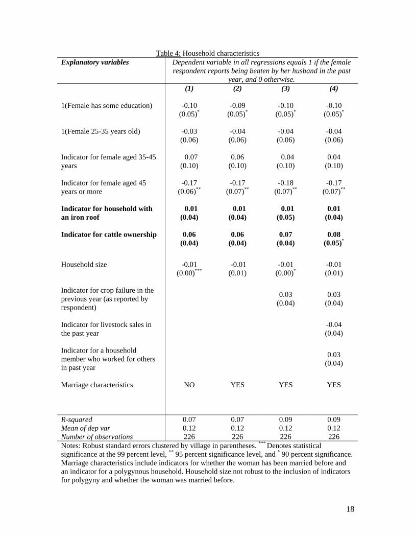
The results in Table 4 include controls for marital characteristics. The signs on the
coefficients are as expected: violence is lower for couples who have been married longer, for
those where the woman “chose” her husband herself, for couples in which the husband stays in
the same house as the wife, and for polygynous households. It is higher for women who have
been married before, as well as couples in which the husband paid bride price to the woman’s
family. However, none of the estimated coefficients are significantly different from zero. There
are obvious endogeneity problems with many of the variables. The number of years married may
be determined in part by whether or not the husband beats his wife, as is the case with the
husband’s primary residence. Although the number of years married is marginally significant in
some specifications, it is not robust to the inclusion of female age categories. The large standard

9
errors on the bride price coefficient may be due to insufficient variation in bride price payment
status once we control for whether the woman has been married before. Marriage payments are
extremely rare for women who have been married before.
There are other possible interpretations of the relationship between age and violence. Sample
selection may play a part. The sample includes only women who are currently married.
Oftentimes, men use violence as a way of “chasing away” their wives. Although wife beating is
common and generally accepted as part of life, both men and women make a distinction between
violence that is “justified” and “excessive”. In community surveys, frequent and severe beatings
were cited as grounds for divorce.
There may be cohort specific levels or trends in domestic violence, or changes over time that
affect all cohorts equally. Disentangling cohort-specific violence from changes over time cannot
be done with a cross-section of data. Moreover, if older women are less likely to report violence –
other things being equal—but just as likely to be victims of violence, the correlation reflects this
bias rather than a true relationship between the two variables. The distinction between the
measures of violence--ever beaten by husband versus beaten in the last year—is informative.
About a quarter of women report being beaten by their spouse at some point in their lives. There
is no relationship between ever beaten and female age. More specifically, the regression-adjusted
prevalence rates for women over 45 years old are not different than those of younger women.
This provides evidence against reporting bias as well as cohort specific levels of violence. In
terms of time trends, it is unlikely—but possible—that domestic violence has been increasing
over time in rural Tanzania.
6.2 Income and violence
There is no systematic relationship between violence and measures of household wealth.
Table 5 presents the results for specifications that include indicators of iron roof and cattle
ownership as proxies for household wealth. The estimated coefficient on the iron roof indicator is
small in magnitude, while cattle ownership is associated with a 6 percent increase in the
probability of violence, though neither is significantly different from zero.
Asset ownership, as measured by cattle and iron roof ownership, may be a good measure
of wealth, but not necessarily of vulnerability. Measures of economic vulnerability are usually
based on variability of income or consumption. It is not possible for me to construct these
measures. Instead, I include indicators for the types of coping mechanisms reported in the
household survey. Specification (3) includes an indicator for whether the household experienced
crop failure in the year before the survey (as reported by the household survey respondent). The
coefficient is positive, but not significant. In (4), I include indicator variables for the two most

10
commonly reported coping mechanisms. In the face of food shortages, people reported selling
livestock and working temporarily for others (usually in exchange for food) as coping
mechanisms. The estimated coefficients are not different from zero. Interestingly, cattle
ownership is marginally significant once the vulnerability measures are introduced.
Women who never attended school are more likely to be victims of violence.
Specifically, women with some education are 10 percent less likely to be victims of violence than
those without any education, though the coefficient is only marginally significant (10 percent
confidence level). The regressions include an indicator for some schooling rather than a
continuous variable because most women either have no education, or if they did attend school,
complete primary. It is problematic to interpret the coefficient of education as causal. Parents
who sent their daughters to school might be better off economically and more committed to their
daughter’s future wellbeing. This may be related to their ability to find a good match for her in
the marriage market, or to intervene and protect their daughter if her husband is violent.
6.3 Social networks and violence
The challenge in trying to disentangle the relationship between social capital and
domestic violence is dealing with the endogeneity of social networks. Cleary, social interaction is
not random. In that sense, relationships with relatives are less problematic than relationships with
friends, since they depend more on household structure than individual choices.
In this case, social networks are measured as the five friends and five relatives with
whom the woman speaks most frequently. Most, but not all, respondents were able to name five
friends and five relatives (referred to as “links”). I include a control for the total number of links
named by the respondent in the regressions. The results presented in Table 6 suggest that close
female friends and relatives, but not other types of social links, play an important role. In this
case, I define closeness by the frequency of interaction. If the respondent speaks to a friend or
relative on a daily basis, or ever other day, this person is referred to as a “close” link. An
additional close female link (friend or relative) is associated with a 2.4 decrease in the probability
of violence.
As can be seen in Table 7, the coefficient on close female links is being driven by the
woman’s relationship to her relatives, not her friends. Both the gender and the frequency of the
interaction with relatives are important. The coefficient on the number of female relatives is not
significantly different from zero (see spec (1)). An additional close relative is associated with a
3.4 lower probability of violence. Table 8 presents OLS and IV estimates for the relationship
between family networks (relatives) and domestic violence. The IV estimated coefficient is

11
negative and larger in magnitude--an additional close relative is associated with a 4.4 lower
probability of violence--but no longer statistically different from zero.
The current specifications do not make a distinction between the woman’s kin and her
husband’s family, or the nature of her relationship to the link (sister-in-law, co-wife, daughter-in-
law). This data is available and will be incorporated in a future version of the paper. It may shed
some light on the mechanism by which relatives, or female relatives, reduce the probability of
violence.
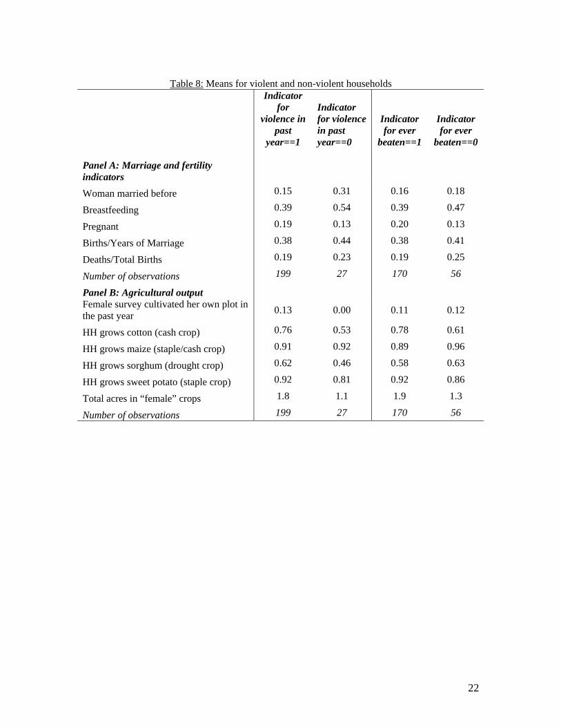
6.3 Domestic violence and other welfare outcomes
There is suggestive evidence for differences in fertility, infant mortality and agricultural
production for violent and non-violent households. Clearly violence is not randomly assigned in
the population, so differences in means cannot be interpreted as the causal effect of violence.
Nevertheless, violent households seem to be worse off along a number of dimensions, which
supports the idea that there are fundamental differences in the way these households allocate
resources.
Table 9 presents averages for violent and non-violent households (column 1 presents
means by whether the woman was beaten in the past year, column 2 presents averages by whether
the woman was ever beaten). Women who report being victims of violence in the previous year
do not cultivate their own plot, while 13 percent of women in non-violent households report
doing so. Violent households also cultivate fewer acres of traditionally female crops, such as
sweet potato and peas. Moreover, women in violent households are more likely to report that
they are largely responsible for cultivating crops that are owned by men, such as maize and
cotton. Though there are no differences in child mortality for the subset of women who report
being beaten in the past year, there are higher rates of child mortality (both the number and the
share of total births) in households in which women report being beaten sometime in the past.
7 Conclusions and Future Work
7.1 Conclusions
This paper finds that individual female characteristics are important predictors of
domestic violence in rural Tanzania. Women are more likely to be victims of spousal violence
during their childbearing years. I argue that this is related to structure of the marriage contract,
which links men’s right over women’s productive labor to their reproductive capacities. There is
also suggestive evidence that close relationships to female relatives, but not friends, play an
important part in reducing violence. There is no systematic relationship between violence and
measures of household wealth. .

12
There is also suggestive evidence that the underlying process of intra-household resource
allocation differs for violent households. This is consistent with the proposition in the theoretical
literature on bargaining that it is inappropriate to model outcomes as Pareto optimal allocations
for violent households. The analysis also highlights the need for a more comprehensive
theoretical framework to address the interrelated processes of intra-household decision-making,
marital formation and dissolution.
7.2 Proposed Extension: A Two-Period Panel
It is possible for me to return to Tanzania in the spring semester to collect another round
of data. This would allow me to ask explicitly about a number of issues that the original survey
did not address, including alcohol consumption, the gender composition of births to each woman,
and the prevalence of polygynous marriages. I could use this additional data and the panel
dimension in my identification strategy.
The literature on domestic violence consistently finds a link between substance abuse and
violence. Although the 2002 survey did not ask explicitly about alcohol consumption, it was
mentioned often in open-ended questions as a source of conflict between spouses (I am currently
coding these responses to obtain a rough—albeit imperfect-- measure of alcohol consumption.)
However, psychologists relate both the propensity towards substance abuse and violence to
(unobservable) personality traits. I could potentially use distance to the closest bar or home
brewery as an instrument for alcohol consumption to identify the relationship between alcohol
use and violence.
There is discursive, but not demographic, evidence for son preference in Africa. I could
further explore the link between violence and fertility by examining the relationship between the
gender composition of births and the prevalence of violence. In contrast to the total number of
births, the gender composition is not determined endogenously. The original survey asked
explicitly about the number of births to each woman, but not the gender composition of births. In
some cases, I can infer the gender composition from the household structure. However, this is
going to be measured with error. For example, it will underestimate the number of female adult
children, since women move away when they marry.
Identification of the relationship between income or wealth and violence is difficult due
to the endogeneity issues. This last year in Meatu District was particularly difficult: excessive
rains resulted in widespread crop failures and hunger. However, villages were differentially
affected by the weather shock. I could use this weather shock as a source of exogenous variation
in income, either at the household or village level.

13
Finally, existing data allows me to determine whether there is a co-wife in the same
household as the family survey respondent, but I do not have information on whether the husband
has other wives in different households. A second round of surveys would allow me to identify all
polygynous households, and also ask about the rank of the wide being interviewed. First wives
have higher status than subsequent wives, so rank may is meaningful. The data would also
include information on health and education outcomes of children, and health outcomes for
adults.
The model to be estimated is given by:
(2) Yijt= Σk βk Xijtk + ΣnδnHijt
n+ Σsγ sVjs + εijt,
and εijt = µi +ηijt
Where εijt has a household specific, time invariant component, µi, and ηijt is assumed to
be uncorrelated with the explanatory variables. If the time invariant component of the error term,
µi, is correlated with the regressors, estimating a model of first-differences (fixed effects) yields
unbiased estimates of the coefficients. The model estimated then becomes (dropping the
subscripts for clarity):
∑ ∆+∆+∆=∆n
nn WaY εθ
Where Wi is the i-th individual or household characteristics that varies over time. More
specifically, the first differences version of the current cross-sectional specification is given by:
)()(
))()(()(
))()(()()()(
12125
124123
1221211212
ijijijij
ijijijij
ijijijijijij
pHHsocialcapHHsocialca
HHAssetsIHHAssetsIHHsizeHHsize
PolygynyIPolygynyINetworksNetworksaaYY
ηηθθθ
θθ
−+−+
−+−+
−+−+−=−
Collecting another round of data would allow me to address econometric issues of
omitted variable bias from the exclusion of unobserved time-invariant household characteristics,
and sample selection. Since there is only one couple surveyed per household, no distinction can
be made between individual, couple and household time-invariant characteristics. That is, µi can
be thought of as including male and female personality traits as well as any family or household
characteristics that do not change over time. In terms of sample selection, the current sample
includes only married women. The panel also offers the possibility of getting a sense of the
sample selection, by comparing changes over time in the rate of separation for violent and non-
violent households.
In order to estimate the first-differences model it is necessary to have variation over time
in the prevalence of violence within households. That is, estimation relies on the existence of
“switchers”: households that report violence in the first period but do not report it in the second

14
period, and vice versa. It is also necessary to have variation in the explanatory variables. In terms
of individual characteristics, I do not expect to see variation in education levels. In rural
Tanzania, both men and women marry once they have completed their education. There is no
variation in the change in age between the two periods, so age would also be excluded from the
first-differences model. Other than the prevalence of polygyny, the remaining marriage
characteristics do not change over time. As is the case with age, the change in the number of
years married will not vary across households.
Individual social networks may vary over time. However, the panel dimension does not
change the problem of potential endogeneity of social networks. In fact, finding a source of
exogenous variation to instrument the change in social networks seems more problematic.
Currently, I instrument social networks using distance to parents’ home, and household structure
(for example, the presence of a woman over forty). The former does not vary over time, while
the latter may be a weak instrument if there is not much variation in household structure over this
period of time.
A random effects estimator would exploit the variation between and within households,
but requires the assumption that the time-invariant component of the error term be uncorrelated
with the explanatory variables. Estimating model (2) in this way makes it possible to distinguish
between age and cohort effects, by including dummies for age and cohort. More generally, the
random effects model allows for the inclusion of household and individual characteristics that are
time invariant, and can be estimated even if there are no within-household changes in the reports
of violence between the two periods.

15
Table 1: Descriptive statistics
Mean Std. dev. N
Panel A: Individual characteristics
Beaten by husband in past year 0.12 0.32 226
Ever beaten by husband 0.26 0.44 226
Female age 33.3 12.2 226
Female education, years 3.7 3.4 226
Female height, cm. 159.5 6.1 211
Male age 39.8 13.6 199
Male education, years 4.5 3.2 218
Male height, cm. 168.4 7.6 144
Panel B: Marriage characteristics
Number of years married 13.2 11.5 226
Woman married before, proportion 0.17 0.38 226
Husband stays in the same house, proportion 0.94 0.24 221
Husband paid bride price, proportion 0.84 0.36 226
Woman chose husband herself, proportion 0.92 0.28 226
Panel C: Household characteristics
Households with an iron roof, proportion 0.27 0.44 226
Household owns cattle, proportion 0.44 0.50 226
Household size 7.9 4.4 226
Household sold livestock in the past year, proportion 0.39 0.49 226
Household member worked for others in the past year, prop 0.41 0.49 226
Panel D: Community characteristics
Number of active women’s groups in village 1.1 1.8 226 Number of other active community groups in village 7.5 5.9 226 Proportion of women in Village Council 0.24 0.06 226 Panel E: Social capital Female member of women’s group in household, proportion 0.12 0.32 226 Female community group memberships 1.3 1.1 226 Male community group memberships 1.7 1.1 226 Household community group memberships 2.0 1.2 226 # of female links 6.7 2.3 226 # of links with whom woman speaks every other day 6.6 2.7 226 # of female links with whom woman speaks every other day 5.2 2.3 226 # of male links with whom woman speaks every other day 1.4 1.4 226 # of links in same village 6.8 2.7 226 # of links with whom woman exchanged gifts in past year 1.2 1.6 226 Total # of links 9.3 2.4 226
16
Table 2: Domestic violence and individual characteristics
Explanatory variables Dependent variable in all regressions is a binary variable that equals 1 if the female respondent reports being beaten by her
husband in the past year, and 0 otherwise. (1) (2) (3) (4) (5) (6) Indicator for (some) female schooling
-0.09 (0.05)*
-0.07 (0.06)
-0.09 (0.05)*
-0.08 (0.06)
-0.06 (0.06)
Indicator for (some) male schooling
-0.06 (0.06)
-0.07 (0.06)
Indicator for female aged 25-35
-0.03 (0.06)
-0.05 (0.06)
-0.03 (0.06)
-0.04 (0.06)
-0.06 (0.07)
Indicator for female aged 35-45
0.07 (0.10)
0.09 (0.11)
0.07 (0.10)
0.05 (0.11)
0.05 (0.12)
Indicator for female aged 45 or above
-0.16 (0.06) **
-0.18 (0.06)***
-0.16 (0.06)**
-0.15 (0.07)**
-0.15 (0.10)
Indicator for male aged 25-35
0.09
(0.08) 0.08
(0.07) Indicator for male aged 35-45
0.06
(0.08) 0.07
(0.07) Indicator for male aged 45 or above
0.04
(0.10) 0.01
(0.07) Female height, cm
0.002
(0.004)
Household Income Proxies NO NO YES NO NO NO R-squared 0.05 0.06 0.05 0.04 0.05 0.01 Mean of dep. var. Std dev of dep. var.
0.12 (0.32)
0.12 (0.32)
0.12 (0.32)
0.12 (0.32)
0.12 (0.32)
0.12 (0.32)
Number of obs 226 211 226 199 199 199 Notes: Robust standard errors clustered by village in parentheses. *** Denotes statistical
significance at the 99 percent level, ** 95 percent significance level, and * 90 percent significance. Also ran the specifications using differences (male – female). The coefficients on the differences
were not significantly different from zero at traditional levels.

17
Table 3: Marriage characteristics Explanatory variables Dependent variable in all regressions equals 1 if the female
respondent reports being beaten by her husband in the past year, and 0 otherwise.
(1) (2) (3) (4) Indicator for female schooling -0.08
(0.05) -0.08 (0.05)
-0.05 (0.05)
-0.05 (0.05)
Number of years married -0.003
(0.002) -0.003
(0.002)* -0.002 (0.002)
-0.002 (0.002)
Indicator for woman married before
0.12 (0.08)
0.12 (0.08)
0.13 (0.08)
0.13 (0.08)
Indicator for polygynous household
-0.04 (0.06)
-0.04 (0.07)
-0.04 (0.06)
-0.05 (0.07)
1(Payment of bride price)
0.05
(0.07) 0.04
(0.08) 1(Husband stays in the same house)
-0.03 (0.09)
-0.03 (0.09)
1(Woman chose husband herself)
-0.10 (0.10)
-0.09 (0.09)
Household Income Proxies NO YES NO YES R-squared 0.04 0.04 0.04 0.04 Mean of dependent variable 0.12 0.12 0.11 0.11 Number of observations 226 226 219 219
Notes: Robust standard errors clustered by village in parentheses. *** Denotes statistical significance at the 99 percent level, ** 95 percent significance level, and * 90 percent significance. Results unchanged if include male schooling in specifications. Household income proxies are indicators for iron roof and cattle ownership at the household level.
18
Table 4: Household characteristics Explanatory variables Dependent variable in all regressions equals 1 if the female
respondent reports being beaten by her husband in the past year, and 0 otherwise.
(1) (2) (3) (4) 1(Female has some education) -0.10
(0.05)* -0.09
(0.05)* -0.10
(0.05)* -0.10
(0.05)* 1(Female 25-35 years old) -0.03
(0.06) -0.04 (0.06)
-0.04 (0.06)
-0.04 (0.06)
Indicator for female aged 35-45 years
0.07 (0.10)
0.06 (0.10)
0.04 (0.10)
0.04 (0.10)
Indicator for female aged 45 years or more
-0.17 (0.06)**
-0.17 (0.07)**
-0.18 (0.07)**
-0.17 (0.07)**
Indicator for household with an iron roof
0.01 (0.04)
0.01 (0.04)
0.01 (0.05)
0.01 (0.04)
Indicator for cattle ownership 0.06
(0.04) 0.06
(0.04) 0.07
(0.04) 0.08
(0.05)*
Household size -0.01 (0.00)***
-0.01 (0.01)
-0.01 (0.00)*
-0.01 (0.01)
Indicator for crop failure in the previous year (as reported by respondent)
0.03
(0.04) 0.03
(0.04)
Indicator for livestock sales in the past year
-0.04 (0.04)
Indicator for a household member who worked for others in past year
0.03
(0.04)
Marriage characteristics NO YES YES YES R-squared 0.07 0.07 0.09 0.09 Mean of dep var 0.12 0.12 0.12 0.12 Number of observations 226 226 226 226 Notes: Robust standard errors clustered by village in parentheses. *** Denotes statistical significance at the 99 percent level, ** 95 percent significance level, and * 90 percent significance. Marriage characteristics include indicators for whether the woman has been married before and an indicator for a polygynous household. Household size not robust to the inclusion of indicators for polygyny and whether the woman was married before.

19
Table 5: Broadening the definition of capital Dependent variable in all regressions is a binary variable that equals 1 if the female respondent
reports being beaten IN THE PAST YEAR by her husband, and 0 otherwise. Explanatory variables (1) (2) (3) (4) (5) (6) Number of female links (friends and relatives)
-0.013 (0.012)
Number of links with whom the woman speaks at least every other day
-0.016 (0.011)
Number of female links with whom the woman speaks at least every other day
-0.024
(0.011)**
Number of links who live in the same village
-0.014 (0.011)
Number of female links who live in the same village
-0.018 (0.011)
Number of links with whom the woman exchanged gifts (food, labor or other) in the past year
-0.010 (0.014)
Number of other links (friends and relatives)
-0.008 (0.016)
0.001 (0.014)
0.004 (0.013)
-0.006 (0.013)
-0.002 (0.014)
-0.012 (0.011)
Individual characteristics YES YES YES YES YES YES Marriage characteristics YES YES YES YES YES YES Household characteristics YES YES YES YES YES YES Community characteristics NO NO NO NO NO NO R-squared 0.08 0.09 0.11 0.08 0.10 0.08 Mean of dep. Var. 0.12 0.12 0.12 0.12 0.12 0.12 Number of observations 226 226 226 226 226 226 Notes: Robust standard errors clustered by village in parentheses. *** Denotes statistical significance at the 99 percent level, ** 95 percent significance level, and * 90 percent significance. Marriage characteristics are indicators for whether the woman has been married before and for polygynous household. Household characteristics are household size, an indicator for whether the household has an iron roof, an indicator for cattle ownership. Community characteristics are the proportion of women on the Village Council, the number of women’s groups in the village, and the number of other types of community groups in the village.

20
Table 6: Friends and relatives
Explanatory variables
Dependent variable in all regressions is a binary variable that equals 1 if the female respondent reports being beaten IN THE
PAST YEAR by her husband, and 0 otherwise. (1) (2) (3) (4) Number of female relatives -0.002
(0.018)
Number of female friends -0.014 (0.010)
Number of relatives with whom the woman speaks at least every other day
-0.034
(0.015)**
Number of friends with whom the woman speaks at least every other day
-0.003 (0.013)
Number of female relatives with whom the woman speaks at least every other day
-0.034
(0.016)**
Number of female friends with whom the woman speaks at least every other day
-0.008 (0.011)
Number of female relatives in the same village
-0.042 (0.041)
Number of female friends in the same village
0.012
(0.036) Number of other links to relatives -0.016
(0.018) -0.010 (0.014)
-0.009 (0.014)
-0.039 (0.039)
Number of other links to friends 0.013 (0.028)
0.031 (0.023)
0.032 (0.015)**
0.050 (0.041)
Individual characteristics of woman YES YES YES YES Marriage characteristics YES YES YES YES Household characteristics YES YES YES YES Community characteristics NO NO NO NO R-squared 0.09 0.12 0.11 0.11 Mean of dep. Var. 0.12 0.12 0.12 0.12 Number of observations 226 226 226 226
Notes: Robust standard errors clustered by village in parentheses. *** Denotes statistical significance at the 99 percent level, ** 95 percent significance level, and * 90 percent significance. Individual characteristics are female age and education. Marriage characteristics are indicators for whether the woman has been married before and for polygynous household. Household characteristics are household size, an indicator for whether the household has an iron roof, an indicator for cattle ownership. Community characteristics are the proportion of women on the Village Council, the number of women’s groups in the village, and the number of other types of community groups in the village.

21
Table 7: Family networks and violence
Dependent variable in all regressions is a binary variable that equals 1 if the female respondent reports being beaten IN THE
PAST YEAR by her husband, and 0 otherwise. Explanatory variables OLS IV (1) (2) Number of relatives with whom the woman speaks at least every other day
-0.038 (0.017)**
-0.044 (0.288)
Number of other links to relatives -0.005
(0.015) -0.007 (0.087)
Individual characteristics of woman YES YES Marriage characteristics YES YES Household characteristics YES YES Community characteristics NO NO R-squared 0.09 0.09 Mean of dep. Var. 0.12 0.12 Number of observations 226 226
Notes: In IV specification (2), female links with whom the woman speaks frequently is instrumented with an indicator for whether the woman resided in the same village before getting married. The variable being instrumented is the number of female relatives with whom the woman speaks at least every other day. Robust standard errors clustered by village in parentheses. *** Denotes statistical significance at the 99 percent level, ** 95 percent significance level, and * 90 percent significance. Individual characteristics are female age and education. Marriage characteristics include an indicator for whether the woman has been married before and an indicator for polygynous household. Household characteristics are household size, an indicator for whether the household has an iron roof, and an indicator for cattle ownership. Community characteristics are the proportion of women on the Village Council, the number of women’s groups in the village, and the number of other types of community groups in the village.
22
Table 8: Means for violent and non-violent households
Indicator for
violence in past
year==1
Indicator for violence in past year==0
Indicator for ever
beaten==1
Indicator for ever
beaten==0 Panel A: Marriage and fertility indicators
Woman married before 0.15 0.31 0.16 0.18
Breastfeeding 0.39 0.54 0.39 0.47
Pregnant 0.19 0.13 0.20 0.13
Births/Years of Marriage 0.38 0.44 0.38 0.41
Deaths/Total Births 0.19 0.23 0.19 0.25
Number of observations 199 27 170 56
Panel B: Agricultural output
Female survey cultivated her own plot in the past year
0.13 0.00 0.11 0.12
HH grows cotton (cash crop) 0.76 0.53 0.78 0.61
HH grows maize (staple/cash crop) 0.91 0.92 0.89 0.96
HH grows sorghum (drought crop) 0.62 0.46 0.58 0.63
HH grows sweet potato (staple crop) 0.92 0.81 0.92 0.86
Total acres in “female” crops 1.8 1.1 1.9 1.3
Number of observations 199 27 170 56

23
References
Becker, G.S. (1981) A Treatise on the Family. Cambridge, MA: Harvard University
Press.
Bourguignon, Francois and Chiappori, Pierre Andre. (1994) “The Collective
Approach to Household Behaviour”, in The Measurement of Household Welfare.
Blundell, Richard; Preston, Ian; Walker, Ian, editors. Cambridge University Press, 70-85.
Counts, D.A., Brown, J. K. and Campbell J.C. (eds.), Sanctions and Sanctuary, Cultural
Perspectives on the Beating of Wives, Boulder, CO: Westview Press, 1992.
Deaton, Angus. The Analysis of Household Surveys: A Microeconometric Approach to
Development Policy. Johns Hopkins University Press: Baltimore, MD, 1997.
Deshpande, A. (2002) “Assets versus Autonomy? The Changing Face of the Gender-
Caste Overlap in India,” Feminist Economics 8, 2: 19-35.
Duflo, E. and Udry, C. (2001) “Intrahousehold Resource Allocation in Cote d’Ivoire:
Social Norms, Separate Accounts and Consumption Choices” Manuscript??.
Farmer, A. and Thiefenthaler, J. (1996) “Domestic Violence: The Value of Services as
Signals,” The American Economic Review 86, 2: 274-279.
____________ (1997) “An Economic Analysis of Domestic Violence,” Review of Social
Economy 15, 3: 337-357.
Goldstein, M. and Udry, C. (1999) “Gender and Land Resource Management in Southern
Ghana” Unpublished Manuscript.
Holmboe-Ottesen, G. and Wandel, M., “Gender and Food: Women’s Bargaining Power
and Agricultural Change in a Tanzanian Community”, in Gender and Change in Developing
Countries. Stolen, K. and Vaa, M., editors. Norwegian University Press: Oslo, 1991. Pp. 92-119.
Jesmin, S. and Salway, S. (2000) “Marriage Among the Urban Poor of Dhaka: Instability
and Uncertainty,” Journal of International Development 12: 689-705.
Levinson, D. (1989) Family Violence in Cross-Cultural Perspectives. Newbury Park,
CA: Sage Publications.
Lundberg, S. and Pollak, R. A. (1994) “NonCooperative Bargaining Models of
Marriage”, The American Economic Review 84, 2: 132-137.
Manser, M. and Brown, M. (1979) “Bargaining Analysis of Household Decisions,” in C.
B. Lloyd, E.S. Andrews, and C.L. Gilroy, (eds.) Women in the Labor Force, New York:
Columbia University Press.
_____________ (1980) “Marriage and Household Decision-Making: A Bargaining
Analysis,” International Economic Review, 21: 31-44.

24
McElroy, M. and Horney, J. (1981) “Nash-Bargained Hosuehold Decisions: Toward a
Generalization of the Theory of Demand,” International Economic Review, 22, 2: 333-349.
Mercer, C. (2002) “The Discourse of Maendeleo and the Politics of Women’s
Participation on Mount Kilimanjaro,” Development and Change 33: 101-127.
Morrison, A.R. and Biehl, M. L. (eds.), Too Close to Home. Domestic Violence in the
Americas, Washington DC: Inter-American Development Bank, 1999.
Pagelow, M.D., Woman Battering: Victims and Their Experiences, Beverly Hills: SAGE
Publications, 1984.
Pollak, R.A. (2002) “An Intergenerational Model of Domestic Violence” NBER Working
Paper 9099.
Pollack, R.A. (1994) “For Better of Worse: The Roles of Power in Models of Distribution
within Marriage,” The American Economic Review 84, 2: 148-152.
Thorsen, D. (2002) “We Help Our Husbands! Negotiating the Household Budget in Rural
Burkina Faso,” Development and Change, Vol. 33: 129-146.
Stevenson, B. and Wolfers, J. (2002) “Till Death Do Us Part: The Effects of Divorce
Laws on Suicide, Domestic Violence and Intimate Homicide,” mimeo, Stanford University.
Strauss, M.A. and Gelles, R. J., Physical Violence in American Families: Risk Factors
and Adaptations to Violence in 8,145 Families, New Brunswick: Transaction Publishers, 1990.
Tauchen, H.V., Witte, A.D. and Long, S.K. (1991) “Domestic Violence: A Non-Random
Affair,” International Economic Review 32, 2: 491-511.
____________ (1995) “The Dynamics of Domestic Violence,” The American Economic
Review 85, 2: 414-418.
Udry, C. (1996) “Gender, Agricultural Production, and the Theory of the Household,”
The Journal of Political Economy, vol. 104, Issue 5: 1010-1046.
Walker, L. E. The Battered Woman, New York: Harper & Row, 1979.
Walker, L. E. The Battered Woman Syndrome, New York: Springer Pub.Co.,
1984.
25
Appendix Chart 1: Violence rates by female age
-0.2
-0.1
0
0.1
0.2
0.3
0.4
0.5
0.6
0.7
16-20 21-25 26-30 31-35 36-40 41-45 46-50 51+
Female age categories
Pro
po
rtio
n o
f w
om
en b
eate
n in
th
e p
ast
year