dominik janzing - intelligent systems machine learning problems read hand-written letters/digits...

Inferring causality from passive observations

Dominik Janzing

Max Planck Institute for Intelligent SystemsTubingen, Germany

18.-22. August 2014

1

Outline

1 why the relation between statistics and causality is tricky

2 causal inference using conditional independences(statistical and general)

3 causal inference using other properties of jointdistributions

4 causal inference in time series, quantifying causalstrength

5 why causal problems matter for prediction

1

Part 3: Why causality matters for prediction

• Typical scenarios of machine learningsupervised learning, unsupervised learning, semi-supervisedlearning

• Causality and semi-supervised learning

• Some methods of machine learningsupport vector machines, reproducing kernel Hilbert spaces

• Prediction from many variablesMarkov blanket

• Kind of summary

2

Typical scenarios of machine learning

3

Typical machine learning problems

• read hand-written letters/digits (given as pixel vectors)

• classify the topics of documents (i.e. in the internet)

• predict the structure of proteins from their acid sequence

• classify cell tissue into tumors and healthy tissue from geneexpression data

4

Scenario with i.i.d. data

Task: predict y from x after observing some samples i.i.d. drawnfrom P(X ,Y ).

●●●●●●●●●●●●●●●●●●●●●●●●●●●●●●●●●●●●●●●●●●●●●●●●●●●●●●●●●●●●●●●●●●●●●●●●●●●●●●●●●●●●●●●●●●●●●●●●●

●●●●●●

●●●●

●●●●

●●●●

●●●●

●●●●

●●●●●●●●●●●●●●●●●●●●●●●●●●●●●●●●●●●●●●●●●●●●●●●●●●●●●●●●●●●●●●●●●●●●●●●

●●●●

●●●●

●●●●

●●●●

●●●●

●●●●

●●●●

●●●●●●

●●●●●●

●●●●●●

●●●●●●

●●●●●●

●●●●

●●●●

●●●●

●●●●

●●●●

●●●●

●●●●●●●●●●●●●●●●●●●●●●●●

X

Y

The variables may attain values in a high-dimensional space (e.g.pixel vector in R20·20, gene expression vector in R28,000)

5

Regression and classification

• Regression: continuous label Y

Y

X

f

• Classification: discrete label Y

X1X1

X2

Y=+1

Y=-1

classifier

6

Supervised, unsupervised and semi-supervised learninge.g. Chapelle et al: Semi-supervised learning, MIT press, 2006

Learn to predict Y from X , given some observations. Whichobservations are given?

• supervised learning:some pairs (x1, y1), . . . , (xn, yn)

• unsupervised learning:only unlabelled x-values x1, . . . , xk

• semi-supervised learning (SSL):some pairs (x1, y1), . . . , (xn, yn) and some unlabelled x-valuesxn+1, . . . , xn+k

7

Unsupervised classification

X1X1

X2

separate clusters are believed to correspond to different labels y :

X1X1

X2

Y=+1

Y=-1

classifier

8

Semi-supervised classification

some points are labeled:

X1X1

X2

then we believe even more that the clusters correspond to differentlabels:

X1X1

X2

Y=+1

Y=-1

classifier

unlabeled points tell us position and angle of the hyperplane9

Another example of semi-supervised classification...

source: http://en.wikipedia.org/wiki/Semi-supervised learning

Here, the shape of the clusters tells us something about the shapeof the classifier.

10

Semi-supervised regression

• Given: multi-dimensional X and real-valued Y

• Task: infer function f such that y ≈ f (x)

• Observation: x-values essentially form a lower dimensionalmanifold of a higher dimensional space

X2

X1

11

Semi-supervised smoothness assumption

• Assumption: the map x 7→ f (x) changes smoothly along themanifold

• Hence: the green and the yellow pojnts have the samedistance to the blue one, the green one is more likely to havea similar y

• semi-supervised regression tries to find functions that fit thelabeled data while changing smoothly along the manifold

12

Motivation for semi-supervised learning

• often it’s expensive to get labeled data

• while unlabeled ones are cheap

Examples:

• classify text w.r.t. its topic: labeling needs to be done byhumans. Unlabeled documents are ubiquitous (e.g. in theinternet)

• object recognition on images

13

Causality and semi-supervised learning

14

SSL in Causal and Anti-Causal settings

The task is to predict Y from X

X Y X Y

causal setting: predict effect from causee.g., predict splice sites from DNA sequence

anticausal setting: predict cause from effecte.g, breast tumor classification,

image segmentation

Scholkopf, Janzing, Peters, Sgouritsa, Zhang, Mooij: On causal and anticausal learning, ICML 2012

15

SSL in Causal and Anti-Causal settings

The task is to predict Y from X

X Y X Y

causal setting: predict effect from causee.g., predict splice sites from DNA sequence

anticausal setting: predict cause from effecte.g, breast tumor classification,

image segmentation

SSL pointless because P(X )contains no information about P(Y |X )

SSL can help because P(X ) and P(Y |X )may contain information about each other


16

Known SSL assumptions link P(X ) to P(Y |X )

• SSL smoothness assumption: the function x 7→ E[Y |x ] shouldbe smooth in regions where p(x) is large.

• Cluster assumption: points lying in the same cluster are likelyto have the same Y .

• Low density separation: The decision boundary should lie in aregion where p(x) is small.

The above assumptions can indeed be viewed as linkingproperties of P(X ) to properties of P(Y |X ).

17

Consider classification in causal direction

• Assume X is the cause with some distribution P(X ):

X1X1

X2

• Let Y be binary and P(Y |X ) be some deterministic rule, e.g.,a separating hyperplane. Assume ‘nature chooses’ itindependently of P(X ):

X1X1

X2

X1X1

X2

18

Consider curved clusters...

X1X1

X2

X1X1

X2

why should the shape of the line describing P(Y |X ) care about theshape of P(X )?

19

Recall semi-supervised regression

We said: close points should have similar values f (x) if they have ashort connection along the manifold

20

Can be justified if Y → X

Let Y and X take values in R and R2, respectively and

X = (g1(Y ), g2(Y )) + U ,

where g1, g2 are continuous functions and U is a small noise vector.

if y is close to y ′ then x , x ′ are close along the manifold

(isolines could be like the red lines)

21

Not justified for X→ Y

Choose a function f : R2 → R independent of P(X )

Then the isolines of f are nor related to the manifold on which thex-values lie

22

Does SSL only work in anticausal direction?

Meta-study:

• we searched the literature for empirical results on SSL withreal data

• we decided (after several discussions) whether a data pair iscausal or anticausal or unclear(here strongly confounded pairs were also consideredanticausal)

• it turned out that none of the sucessful cases was causal


23

Semi-supervised classification: 8 benchmark datasets

[O. Chapelle et al., 2006] Semi-Supervised Learning.

g241c g241d Digit1 USPS COIL BCI Text SecStr30

40

50

60

70

80

90

100

Acc

urac

y of

bas

e an

d se

mi−

supe

rvis

ed c

lass

ifier

s

Anticausal/ConfoundedCausalUnclear

Comparison of 11 SSL methods with the base classifiers 1-NN and SVM (star).

• In the causal case (red) the star is below the other points, i.e., SSLperformed worse than methods without SSL

• In the other cases the star is often above the other points, SSL helped.

24

Semi-supervised classification: 8 benchmark datasets

[O. Chapelle et al., 2006] Semi-Supervised Learning.

g241c g241d Digit1 USPS COIL BCI Text SecStr30

40

50

60

70

80

90

100

Acc

urac

y of

bas

e an

d se

mi−

supe

rvis

ed c

lass

ifier

s


Comparison of 11 SSL methods with the base classifiers 1-NN and SVM (star).

• In the causal case (red) the star is below the other points, i.e., SSLperformed worse than methods without SSL

• In the other cases the star is often above the other points, SSL helped.24

Semi-supervised classification: 26 UCI datasets

[Y. Guo et al., 2006] An extensive empirical study on semi-supervised learning.

25

Semi-supervised classification: 26 UCI datasets

ba−scbr−c br−w col col.O cr−a cr−g diab he−che−hhe−s hep ion iris kr−kp lab lett mush seg sick son splic vehi vote vow wave−100

−80

−60

−40

−20

0

20

40

60

Rel

ativ

e de

crea

se o

f err

or w

hen

usin

g s

elf−

trai

ning

inst

ead

a ba

se c

lass

ifier


Comparison of a SSL method with 6 corresponding non-SSL-basedclassifiers.

• all red points are below or on the zero line, i.e., SSL performedworse or equal than all the non-SSL-based methods

• blue and green points are sometime above the line, i.e., SSL helped.

26

to understand how SSL works...

Some basic ideas of machine learning

27

Binary classification

Examples:• distinguish between 0 and 1 from given pixel vectors in hand

written digits• distinguish between healthy cells and tumor cells given the

vector of gene expression levels

y=1

y= 1

?

• given: some training examples (x1, y1), . . . , (xn, yn) withxj ∈ Rk and yj ∈ {−1,+1} (two classes)

• goal: find a function f that separates the two classes• assumption: there is a linear classifier, i.e., an affine f such

that f (xj) > 0 if and only yj = +128

Popular solution: support vector machine Vapnik 1963

see also Scholkopf & Smola: Learning with kernels

choose the hyperplane that maximizes the margin:find w ∈ Rk and b ∈ R that minimize ‖w‖2 subject to

yj(〈w, xj〉+ b) ≥ 1 ∀j = 1, . . . , n

y=1

y= 1

.

29

Support vectors

The support vectors are those xj that lie on the boundary of themargin:

y=1

y= -1

.

support vectors

observations:

• points other than support vectors are irrelevant for theoptimization

• the optimal w lies in the span of the support vectors

30

Soft margin SVMs

Often there is no hyperplane that classifies all points correctly:

y=1

y= -1

error terms(slack variables)

maximize margin while avoiding too large error terms

31

How can we include unlabelled points?

32

Transductive support vector machine

see e.g. Joachims: Transductive support vector machines, 2006

y=1

y= -1

new maximum margin hyperplane

old maximum margin hyperplane

maximize the margin using also the unlabelled points(yields computationally hard optimization problem)

33

Non-linear classification

X1X1

X2

here we need a non-linear function f for classification

In other words: find a function f for which f (xj) > 0 if yj = +1and f (xj) < 0 if yj = −1.

34

Non-linear classification via feature maps

• define a map φ that maps x to non-linear functions of x :

φ(x) :=

f1(x)f2(x)f3(x)...

∈ H

• in this high-dimensional space H, a non-linear function mayturn into a linear one

• example: let x = (x1, x2) ∈ R2 and define

φ(x) :=

(x2

1

x22

).

Then the circle x21 + x2

2 = 1 is given by the linear equation

φ1(x) + φ2(x) = 1

35

‘Powerful’ feature maps

• we don’t need to design a different feature map for everyproblem(for instance one that already knows the classifier)

• it will turn out that there are feature maps that are sopowerful that they can always be used

• idea: choose a map that contains an infinite set of functions,e.g.,

φ(x) =

xx2

x3

.

.

.

.

36

The kernel trick: we don’t need φ itself...

Define the function

k(x, x′) := 〈φ(x), φ(x′)〉 .

• recall optimization problem:minimize ‖w‖2 subject to

yj(〈w, xj〉+ b) ≥ 1 ∀j = 1, . . . , n

• recall that the optimal w can be written as

w =∑j

ajφ(xj)

with some appropriate a

• to classify a new point x we only need to compute∑j

aj〈φ(xj), φ(x)〉 =∑j

ajk(xj , x) .

37

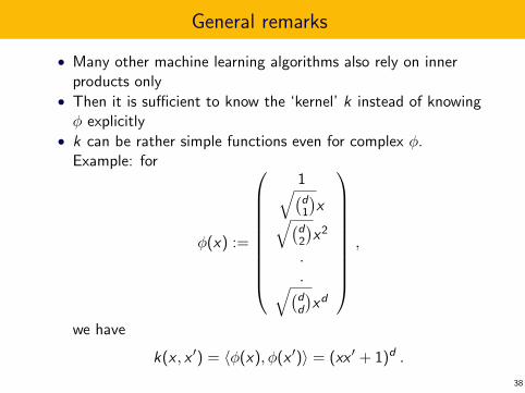
General remarks

• Many other machine learning algorithms also rely on innerproducts only

• Then it is sufficient to know the ‘kernel’ k instead of knowingφ explicitly

• k can be rather simple functions even for complex φ.Example: for

φ(x) :=

1√(d1

)x√(d

2

)x2

.

.√(dd

)xd

,

we have

k(x , x ′) = 〈φ(x), φ(x ′)〉 = (xx ′ + 1)d .

38

Define vector spaces by kernels

Turning around the idea: define a vector space via the kernel.

Question:Given a function

(x , x ′) 7→ k(x , x ′) ,

under which condsitions is there a map φ such that

k(x , x ′) = 〈φ(x), φ(x ′)〉 ?

39

Positive definite functions

Definition

A function k : X × X → R is called a positive definite kernel if forall k ∈ N and any x1, . . . , xk , the matrix k(xi , xj) is positivedefinite, i.e., ∑

ij

cicjk(xi , xj) ≥ 0 ,

for all vectors c ∈ Rk .

Idea: positive definite functions are like positive definite matriceswith continuous index x

40

Feature maps define positive definite kernels

Theorem

Let H be a real-valued vector space with inner product and andφ : X → H be a map then

k(xi , xj) := 〈φ(xi ), φ(xj)〉

is a positive definite kernel

Proof: ∑ij

cicj〈φ(xi ), φ(xj)〉

=

⟨∑i

ciφ(xi ),∑j

cjφ(xj)

⟩≥ 0 .

41

Terminology: Hilbert spaces

• (possibly infinite-dimensional) vector space H• endowed with an inner product

〈., .〉 : H×H → R〈., .〉 : H×H → C

• complete w.r.t. inner product norm, i.e., every Cauchysequence in H has a limit in H

Examples: Cn,Rn, L2(R), `2(N)

42

Defining Hilbert spaces via kernels

Theorem (Proposition 2.14 in Scholkopf & Smola, 2002)

Let X be a topological space and k : X × X → R be a continuouspositive definite kernel, then there exists a Hilbert space H and acontinuous map φ : X → H such that for all x , x ′ ∈ X , we have

k(x , x ′) = 〈φ(x), φ(x ′)〉 .

Hence: feature maps φ define kernels and vice versa

43

Examples for kernels

• Gauss kernel: k : Rn × Rn → R

k(x, x′) := e−‖x−x′‖2

2σ2 .

• polynomial kernel:

k(x, x′) := 〈x, x′〉d

• inhomogeneous polynomial kernel:

k(x, x′) := (〈x, x′〉+ 1)d

44

Reproducing kernel Hilbert space (RKHS)

How to get H from k :

• Every x defines a function fx : X 7→ R via

fx(x ′) := k(x , x ′) .

• Define an inner product by

〈fx , fx ′〉 := k(x , x ′) .

• Let H be the smallest Hilbert space containing all thesefunctions (fx)x∈X with the above inner product

45

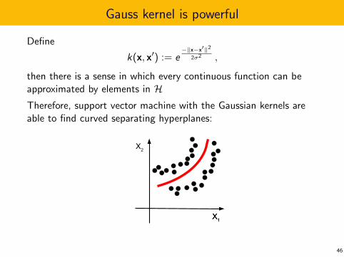
Gauss kernel is powerful

Define

k(x, x′) := e−‖x−x′‖2

2σ2 ,

then there is a sense in which every continuous function can beapproximated by elements in HTherefore, support vector machine with the Gaussian kernels areable to find curved separating hyperplanes:

X1X1

X2

46

Likewise...

Transductive SVM with Gauss kernels is able to find curvedseparating hyperplanes based on the pattern of the unlabeledpoints:

X1X1

X2

47

Applications of SSL

e.g. Nigam et al: Semi-supervised text classification using EM, 2006

Text classification

• task: assign a topic y to a document x in the internet

• given: a few labelled documents (x1, y1), . . . , (xn, yn)(expensive, done by humans), and a huge number ofunlabelled examples xn+1, . . . , xn+k

• idea: different topics correspond to clusters inhigh-dimensional space(x vector of word counts, i.e., x ∈ Nd

0 where d is the size ofthe vocabulary)

48

Prediction from many variables

49

Prediction tasks where causal information may beirrelevant

Health Insurance company asks a costumer before giving acontract:

• age

• job

• hobbies

• address

to determine the risk of getting sick.

It does not matter whether these features are causal or not -properties that correlate with the risk are useful regardless of theyare causes!

50

Markov blanket (set of relevant variables)

• given: causal DAG with nodes X1, . . . ,Xn

• task: predict Xj from all the other variables

• obvious solution: best prediction given by

p(Xj |X1, . . . ,Xj−1,Xj+1, . . . ,Xn) .

• goal: remove irrelevant nodes

• question: what’s the smallest set of variables S such that

Xj ⊥⊥ XS |XS \ Xj ?

• answer: Markov blanket, i.e., the parents and the children ofXj , and the other parents of the latter (if we assumefaithfulness)

51

Proof that Markov blanket is the smallest set

• Let M(j) be the Markov blanket of Xj . Then

Xj ⊥⊥ XM(j) |X ¯M(j) \ Xj , (1)

can be checked via d-separation

• every set S satisfying (1) contains M(j):• no set can d-separate Xj from its parents or children.

Therefore they are contained in S• conditioning on the children of Xj unblocks the path to the

parents of the children, no matter which variables we conditionon

52

Markov blanket Pearl 1988

• Definition via causal terminology:consists of parents, children and further parents of the children

• Definition via predictive relevance:minimal set of variables that render all others irrelevant

Two perspectives:

• Causal structure tells us which variables are irrelevant becausethey are conditionally independent

• Conditional independences tell us causal structure

Argument for causality seems circular!53

Predicting from causes is more robust

B

C

E

V

P(V |C ) predicts V from its cause

(‘causal prediction’)

P(V |E ) predicts V from its effect

(‘anticausal prediction’)

• P(V |E ) changes when background condition B changesbecause V 6⊥⊥ B |E

• P(V |C ) remains constant (‘covariate shift’) since V ⊥⊥ B |C .Scholkopf, Janzing, Peters, Sgouritsa, Zhang, Mooij ICML 2012

54

Kind of summary

55

Two types of asymmetries between cause and effect

• Independence based assumption: P(C ) and P(E |C )contain no information about each other because ‘naturechooses them independently’

• no SSL in causal direction• P(C ) ansd P(E |C ) are algorithmically independent• p(C ) is not particualrly large in regions where f has large slope

(IGCI)

• Occam’s Razor assumption: Decomposition of P(C ,E ) intoP(C )P(E |C ) tends to be simpler than decomposition intoP(E )P(C |E )

• P(E |C ) may be of some simple type, e.g. non-linear additivenoise, while P(C |E ) isn’t

• some Bayesian method not mentioned• K (P(C )) + K (P(E |C )) ≤ K (P(E )) + K (P(C |E ))

56

Relating the two types via a toy model

• choose P(C ) randomly from some finite set Pi (C ) withi = 1, . . . , n

• choose P(E |C ) randomly from some finite set Pj(E |C ) withj = 1, . . . , n

• then Pi (C )Pj(E |C ) defines n2 different distributions Pij(C ,E )

• generically, this yields n2 different distributions Pij(E ) andPij(C |E )

• hence, the backwards conditionals P(E ) and P(C |E ) run overa larger set

57

Future work

find appropriate ways to compare complexities of P(X ),P(Y |X ) toP(Y )P(X |Y )

58

Psychology

Humans intuition about anticausal conditionals P(C |E ) can bepretty bad:

• Consider a random walk on Z• Let Xt be the position at time t

• Let p(Xt+1|Xt) = 1/2 for |Xt+1 − Xt | = 1

• Try to infer p(Xt |Xt+1)

• Many people think it would also be symmetric, i.e., givenXt+1, the two possibilities Xt = Xt+1 ± 1 would be equallylikely

We are used to think in terms of causal conditionals, because theydefine the mechanisms

60

State of the art and outlook

• Asymmetries of cause and effect do exist (at least in the sensethat decision rate above chance level is possible)

• Initial scepticism against the field has decreased

• Try your own ideas, good methods need not build upon theexisting ones

61

Thank you for your attention

62

dominik janzing - intelligent systems machine learning problems read hand-written letters/digits...

Documents