dominique picard antenna measurement - intech - open science open
TRANSCRIPT

Antenna Measurement 193
Antenna Measurement
Dominique Picard
x
Antenna Measurement
Dominique Picard Supélec Plateau de Moulon 91192 Gif sur Yvette Cedex
France
1. Introduction
The antenna is an important element of radiocommunication, remote sensing and radiolocalisation systems. The measurement of the antenna radiation pattern characteristics allows one to verify the conformity of the antenna. The simplest measurement method consists in the direct far-field measurement. For large antennas, the necessary measurement distance raises a problem which was resolved by the introduction of compact ranges and near-field techniques. Compact range consists in a focusing system, as a reflector, which can create a plane wave at short distance. The principle of near-field techniques is to measure the field radiated by an antenna at a short distance on a given surface surrounding the antenna, then to calculate the far-field starting from the measured near-field. These last techniques also make it possible to have an excellent precision as required by the satellite antennas for example. The near-field techniques also make it possible to carry out the diagnosis of the antennas, i.e. to find defects on the antenna. The duration of the measurement of the large antennas, which claims a large number of measurement points, was reduced considerably by the use of rapid near-field assessment system, for which the mechanical displacement of the probe was replaced by the electronic scanning of a probes array.
2. Direct far-field measurement
2.1 Antenna pattern measurement There are four different regions for the electromagnetic field radiated by an antenna: three near-field regions and one far-field region. The nearest region is the reactive field regionwhich extends until a distance of one wavelength from the antenna surface. The second near-field region is the Rayleigh region which extends from the reactive region until a distance D2/(2) from the antenna surface, a relation in which D is the tested antenna diameter. The third near-field region is the Fresnel region which extends from D2/(2) until 2D2/ from the antenna surface. The last region is the far-field Fraunhofer region which starts at a distance of 2D2/. The space variations of the electromagnetic field differ in these four regions. It is thus necessary to be at a distance sufficient (>2D2/) to carry out direct far-field measurements.
10
www.intechopen.com

Microwave and Millimeter Wave Technologies: Modern UWB antennas and equipment 194
Fig. 1. Different field regions for a large antenna Direct far-field measurement can be realized either in indoor or outdoor range (Kummer & Gillepsie, 1978). Indoor range consists in an anechoic chamber with one source antenna and the tested antenna placed on a positioner. This positioner allows one to vary the tested antenna attitude with respect to the direction of the wave incidence of the wave for far-field pattern measurement. Outdoor range consists in a tower bearing a source antenna and the tested antenna placed on a positioner. The distance between the two antennas can be larger for outdoor range, i.e. the capacity of outdoor range in terms of tested antenna dimensions is higher. On the other hand the outdoor range is sensitive to parasitic signals and ground reflections. Indoor range Outdoor range Fig. 2. Different range geometries
2.2 Measurement of the characteristics of the pattern Gain measurement Absolute gain measurements use power budget between antennas. The Friis transmission formula gives a relation between the gains GA and GB of two antennas A and B: Pr = Pi GA GB (/4r)2 (1)
Pr is the power received at a matched load connected to the receiving antenna, Pi the power accepted by the transmitting antenna, is the wavelength and r the distance between the two antennas. The use of this formula requires that the two antennas A and B are
D2/(2) 2D2/r
reactive Rayleigh Fresnel Fraunhofer
D
polarization matched and that the separation distance between the antennas corresponds to far-field conditions. Fig. 3. The two antennas system corresponding to the Friis formula The first method uses the tested antenna and a reference antenna with a known gain. The measurements of Pr, Pi, r, and the knowledge of give the value of the tested antenna gain by means of the Friis formula. The second method used two identical tested antennas with the same gain. The Friis formula gives the value of the tested gain antenna starting from the same measurements as the preceding method. The third method used three antennas A, B and C, generally the tested antenna and two other antennas. Three different power budgets are carried out, with the three possible antennas pairs leading to the three following equations:
GA GB = (Pr/Pi)AB (4r/)2 (2) GB GC = (Pr /Pi)BC (4r/)2 (3) GC GA = (Pr /Pi)CA (4r/)2 (4)
These three formulas provide the determination of the three different gains GA , GB and GC. Directivity measurement There are two methods which make it possible to measure the directivity Dir of an antenna. The first method is based on the definition of the directivity. The knowledge of the relative far-field radiated by the antenna in all the directions is sufficient to know the directivity of this antenna. This method is called the pattern integration method because it uses the integration of the radiated power density (dPe/dS) on all the directions to calculate the total power radiated by the antenna Pe. The power density is related to the electric field E at a distance r by the relation:
(dPe/dS) = E2/Z0 (5)
Z0 = 120 is the free space impedance of wave.
Pe =
0
2
0 (dPe/dS) r sin d d (6)
Dir = (dPe/dS) / [Pe/(4r2)] (7)
Pi Pr
r
Transmitting antenna Receiving antenna
www.intechopen.com

Antenna Measurement 195
Fig. 1. Different field regions for a large antenna Direct far-field measurement can be realized either in indoor or outdoor range (Kummer & Gillepsie, 1978). Indoor range consists in an anechoic chamber with one source antenna and the tested antenna placed on a positioner. This positioner allows one to vary the tested antenna attitude with respect to the direction of the wave incidence of the wave for far-field pattern measurement. Outdoor range consists in a tower bearing a source antenna and the tested antenna placed on a positioner. The distance between the two antennas can be larger for outdoor range, i.e. the capacity of outdoor range in terms of tested antenna dimensions is higher. On the other hand the outdoor range is sensitive to parasitic signals and ground reflections. Indoor range Outdoor range Fig. 2. Different range geometries
2.2 Measurement of the characteristics of the pattern Gain measurement Absolute gain measurements use power budget between antennas. The Friis transmission formula gives a relation between the gains GA and GB of two antennas A and B: Pr = Pi GA GB (/4r)2 (1)
Pr is the power received at a matched load connected to the receiving antenna, Pi the power accepted by the transmitting antenna, is the wavelength and r the distance between the two antennas. The use of this formula requires that the two antennas A and B are
D2/(2) 2D2/r
reactive Rayleigh Fresnel Fraunhofer
D
polarization matched and that the separation distance between the antennas corresponds to far-field conditions. Fig. 3. The two antennas system corresponding to the Friis formula The first method uses the tested antenna and a reference antenna with a known gain. The measurements of Pr, Pi, r, and the knowledge of give the value of the tested antenna gain by means of the Friis formula. The second method used two identical tested antennas with the same gain. The Friis formula gives the value of the tested gain antenna starting from the same measurements as the preceding method. The third method used three antennas A, B and C, generally the tested antenna and two other antennas. Three different power budgets are carried out, with the three possible antennas pairs leading to the three following equations:
GA GB = (Pr/Pi)AB (4r/)2 (2) GB GC = (Pr /Pi)BC (4r/)2 (3) GC GA = (Pr /Pi)CA (4r/)2 (4)
These three formulas provide the determination of the three different gains GA , GB and GC. Directivity measurement There are two methods which make it possible to measure the directivity Dir of an antenna. The first method is based on the definition of the directivity. The knowledge of the relative far-field radiated by the antenna in all the directions is sufficient to know the directivity of this antenna. This method is called the pattern integration method because it uses the integration of the radiated power density (dPe/dS) on all the directions to calculate the total power radiated by the antenna Pe. The power density is related to the electric field E at a distance r by the relation:
(dPe/dS) = E2/Z0 (5)
Z0 = 120 is the free space impedance of wave.
Pe =
0
2
0 (dPe/dS) r sin d d (6)
Dir = (dPe/dS) / [Pe/(4r2)] (7)
Pi Pr
r
Transmitting antenna Receiving antenna
www.intechopen.com

Microwave and Millimeter Wave Technologies: Modern UWB antennas and equipment 196
The second method uses the relation between the directivity Dir and the gain G of a given antenna: Dir = G/ (8)
in which s the efficiency of the antenna. The measurements of the gain and the efficiency of the antenna result in the knowledge of the directivity. The first method is used more for directive antennas while the second is rather used more for omnidirectional antennas. Efficiency There are essentially three different methods to measure the efficiency of an antenna. The first method consists in the measurement of the gain G and the directivity D of the antenna, and then the relation between gain, directivity and efficiency results in to obtain the efficiency: = G/Dir (9)
The second method uses the measurement of the antenna input impedance and is called the Wheeler Cap Method. For certain antennas, microstrip patches for example, the losses can be modeled by a series resistance or a parallel resistance Rl with the antenna input resistance Rr. Two different antenna input impedance measurements are performed. The first measurement is done with the antenna in free space and the second measurement with the antenna inside a metallic hemisphere, and the input resistance of the antenna takes the values R1 and R2 respectively for these two measurements. If the loss resistance occurs in series, then it is short-circuited by the cap, and if the loss resistance occurs in parallel, then it is open-circuited by the cap. It is possible to have the relation between the efficiency, the radiated power and the losses power. This relation allows one to obtain the efficiency in function of Rr and Rl and then in function of the measured input resistance R1 and R2. For the series modelling the efficiency is:
= Rr/( Rr + Rl) = (R1 - R2)/R1 (10) And for the parallel modelling:
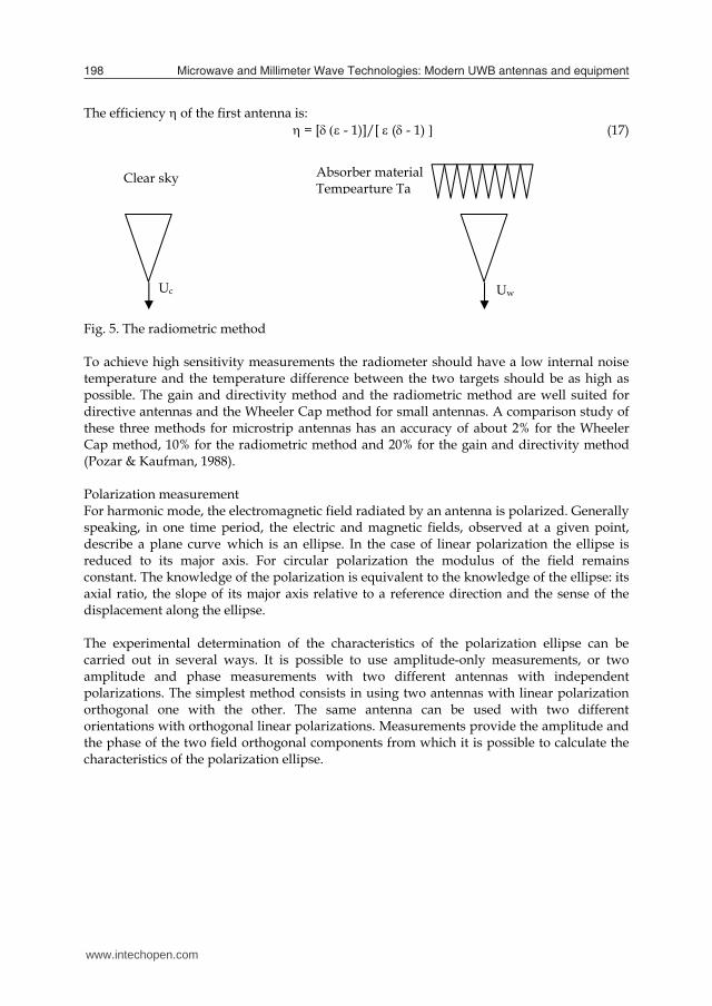
= Rl/( Rr + Rl) = (R2 – R1)/R2 (11) The third method is called radiometric method. It consists in the measurement of the available noise power at the output of the antenna by means of a radiometer (Ashkenazy et al, 1985). This power U is related to the effective temperature Te of the antenna and the equivalent temperature Tn of the radiometer by:
U = C(Te + Tn) (12)
in which C is a constant. The equivalent temperature Tn is derivated from the noise figure of the radiometer. The effective temperature Te of the antenna, at physical temperature Ta, is related to the efficiency of the antenna by:
Te = Ta (1-) + Tt (13) Fig. 4. The Wheeler Cap Method Tt is the temperature target aimed by the antenna. The measurement of the noise power U for two different target temperatures, respectively the cold temperature Tc and the warm temperature Tw, allows the determination of the efficiency . The cold target temperature is a clear sky and the warm one is an extended absorber at room temperature Ta.
= [(Tn + Ta)(1 - )]/ [ (Tc + Ta)] (14)
= Uc/Uw (15) In fact it is also better to measure another antenna with high efficiency, such as a horn, for which the efficiency is equal to 1, with the same cold and warm temperatures as the first antenna. For this second antenna:
Uc/Uw = = (Tn + Ta)/ (Tn + Tc) (16)
RE =R2
Metallic cap
Ground plane
RE =R1
Free space
Ground plane
Rl Rr
Series model
Rl Rr
Parallel model
www.intechopen.com

Antenna Measurement 197
The second method uses the relation between the directivity Dir and the gain G of a given antenna: Dir = G/ (8)
in which s the efficiency of the antenna. The measurements of the gain and the efficiency of the antenna result in the knowledge of the directivity. The first method is used more for directive antennas while the second is rather used more for omnidirectional antennas. Efficiency There are essentially three different methods to measure the efficiency of an antenna. The first method consists in the measurement of the gain G and the directivity D of the antenna, and then the relation between gain, directivity and efficiency results in to obtain the efficiency: = G/Dir (9)
The second method uses the measurement of the antenna input impedance and is called the Wheeler Cap Method. For certain antennas, microstrip patches for example, the losses can be modeled by a series resistance or a parallel resistance Rl with the antenna input resistance Rr. Two different antenna input impedance measurements are performed. The first measurement is done with the antenna in free space and the second measurement with the antenna inside a metallic hemisphere, and the input resistance of the antenna takes the values R1 and R2 respectively for these two measurements. If the loss resistance occurs in series, then it is short-circuited by the cap, and if the loss resistance occurs in parallel, then it is open-circuited by the cap. It is possible to have the relation between the efficiency, the radiated power and the losses power. This relation allows one to obtain the efficiency in function of Rr and Rl and then in function of the measured input resistance R1 and R2. For the series modelling the efficiency is:
= Rr/( Rr + Rl) = (R1 - R2)/R1 (10) And for the parallel modelling:
= Rl/( Rr + Rl) = (R2 – R1)/R2 (11) The third method is called radiometric method. It consists in the measurement of the available noise power at the output of the antenna by means of a radiometer (Ashkenazy et al, 1985). This power U is related to the effective temperature Te of the antenna and the equivalent temperature Tn of the radiometer by:
U = C(Te + Tn) (12)
in which C is a constant. The equivalent temperature Tn is derivated from the noise figure of the radiometer. The effective temperature Te of the antenna, at physical temperature Ta, is related to the efficiency of the antenna by:
Te = Ta (1-) + Tt (13) Fig. 4. The Wheeler Cap Method Tt is the temperature target aimed by the antenna. The measurement of the noise power U for two different target temperatures, respectively the cold temperature Tc and the warm temperature Tw, allows the determination of the efficiency . The cold target temperature is a clear sky and the warm one is an extended absorber at room temperature Ta.
= [(Tn + Ta)(1 - )]/ [ (Tc + Ta)] (14)
= Uc/Uw (15) In fact it is also better to measure another antenna with high efficiency, such as a horn, for which the efficiency is equal to 1, with the same cold and warm temperatures as the first antenna. For this second antenna:
Uc/Uw = = (Tn + Ta)/ (Tn + Tc) (16)
RE =R2
Metallic cap
Ground plane
RE =R1
Free space
Ground plane
Rl Rr
Series model
Rl Rr
Parallel model
www.intechopen.com
Microwave and Millimeter Wave Technologies: Modern UWB antennas and equipment 198
The efficiency of the first antenna is: = [ - 1)]/[ (- 1) (17)
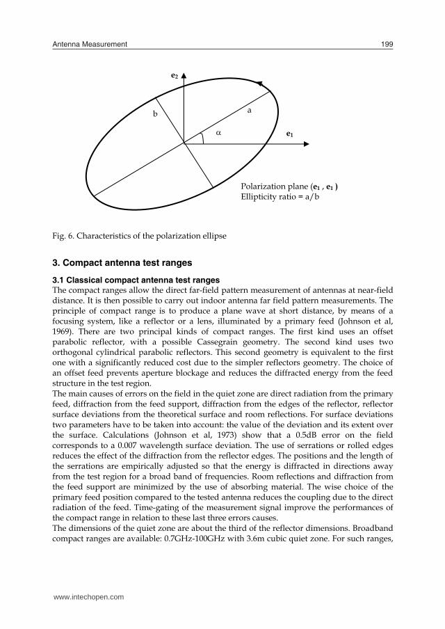
Fig. 5. The radiometric method To achieve high sensitivity measurements the radiometer should have a low internal noise temperature and the temperature difference between the two targets should be as high as possible. The gain and directivity method and the radiometric method are well suited for directive antennas and the Wheeler Cap method for small antennas. A comparison study of these three methods for microstrip antennas has an accuracy of about 2% for the Wheeler Cap method, 10% for the radiometric method and 20% for the gain and directivity method (Pozar & Kaufman, 1988). Polarization measurement For harmonic mode, the electromagnetic field radiated by an antenna is polarized. Generally speaking, in one time period, the electric and magnetic fields, observed at a given point, describe a plane curve which is an ellipse. In the case of linear polarization the ellipse is reduced to its major axis. For circular polarization the modulus of the field remains constant. The knowledge of the polarization is equivalent to the knowledge of the ellipse: its axial ratio, the slope of its major axis relative to a reference direction and the sense of the displacement along the ellipse. The experimental determination of the characteristics of the polarization ellipse can be carried out in several ways. It is possible to use amplitude-only measurements, or two amplitude and phase measurements with two different antennas with independent polarizations. The simplest method consists in using two antennas with linear polarization orthogonal one with the other. The same antenna can be used with two different orientations with orthogonal linear polarizations. Measurements provide the amplitude and the phase of the two field orthogonal components from which it is possible to calculate the characteristics of the polarization ellipse.
Clear sky Absorber material Tempearture Ta
Uw Uc
Fig. 6. Characteristics of the polarization ellipse
3. Compact antenna test ranges
3.1 Classical compact antenna test ranges The compact ranges allow the direct far-field pattern measurement of antennas at near-field distance. It is then possible to carry out indoor antenna far field pattern measurements. The principle of compact range is to produce a plane wave at short distance, by means of a focusing system, like a reflector or a lens, illuminated by a primary feed (Johnson et al, 1969). There are two principal kinds of compact ranges. The first kind uses an offset parabolic reflector, with a possible Cassegrain geometry. The second kind uses two orthogonal cylindrical parabolic reflectors. This second geometry is equivalent to the first one with a significantly reduced cost due to the simpler reflectors geometry. The choice of an offset feed prevents aperture blockage and reduces the diffracted energy from the feed structure in the test region. The main causes of errors on the field in the quiet zone are direct radiation from the primary feed, diffraction from the feed support, diffraction from the edges of the reflector, reflector surface deviations from the theoretical surface and room reflections. For surface deviations two parameters have to be taken into account: the value of the deviation and its extent over the surface. Calculations (Johnson et al, 1973) show that a 0.5dB error on the field corresponds to a 0.007 wavelength surface deviation. The use of serrations or rolled edges reduces the effect of the diffraction from the reflector edges. The positions and the length of the serrations are empirically adjusted so that the energy is diffracted in directions away from the test region for a broad band of frequencies. Room reflections and diffraction from the feed support are minimized by the use of absorbing material. The wise choice of the primary feed position compared to the tested antenna reduces the coupling due to the direct radiation of the feed. Time-gating of the measurement signal improve the performances of the compact range in relation to these last three errors causes. The dimensions of the quiet zone are about the third of the reflector dimensions. Broadband compact ranges are available: 0.7GHz-100GHz with 3.6m cubic quiet zone. For such ranges,
a b
Polarization plane (e1 , e1 ) Ellipticity ratio = a/b
e1
e2
www.intechopen.com
Antenna Measurement 199
The efficiency of the first antenna is: = [ - 1)]/[ (- 1) (17)
Fig. 5. The radiometric method To achieve high sensitivity measurements the radiometer should have a low internal noise temperature and the temperature difference between the two targets should be as high as possible. The gain and directivity method and the radiometric method are well suited for directive antennas and the Wheeler Cap method for small antennas. A comparison study of these three methods for microstrip antennas has an accuracy of about 2% for the Wheeler Cap method, 10% for the radiometric method and 20% for the gain and directivity method (Pozar & Kaufman, 1988). Polarization measurement For harmonic mode, the electromagnetic field radiated by an antenna is polarized. Generally speaking, in one time period, the electric and magnetic fields, observed at a given point, describe a plane curve which is an ellipse. In the case of linear polarization the ellipse is reduced to its major axis. For circular polarization the modulus of the field remains constant. The knowledge of the polarization is equivalent to the knowledge of the ellipse: its axial ratio, the slope of its major axis relative to a reference direction and the sense of the displacement along the ellipse. The experimental determination of the characteristics of the polarization ellipse can be carried out in several ways. It is possible to use amplitude-only measurements, or two amplitude and phase measurements with two different antennas with independent polarizations. The simplest method consists in using two antennas with linear polarization orthogonal one with the other. The same antenna can be used with two different orientations with orthogonal linear polarizations. Measurements provide the amplitude and the phase of the two field orthogonal components from which it is possible to calculate the characteristics of the polarization ellipse.
Clear sky Absorber material Tempearture Ta
Uw Uc
Fig. 6. Characteristics of the polarization ellipse
3. Compact antenna test ranges
3.1 Classical compact antenna test ranges The compact ranges allow the direct far-field pattern measurement of antennas at near-field distance. It is then possible to carry out indoor antenna far field pattern measurements. The principle of compact range is to produce a plane wave at short distance, by means of a focusing system, like a reflector or a lens, illuminated by a primary feed (Johnson et al, 1969). There are two principal kinds of compact ranges. The first kind uses an offset parabolic reflector, with a possible Cassegrain geometry. The second kind uses two orthogonal cylindrical parabolic reflectors. This second geometry is equivalent to the first one with a significantly reduced cost due to the simpler reflectors geometry. The choice of an offset feed prevents aperture blockage and reduces the diffracted energy from the feed structure in the test region. The main causes of errors on the field in the quiet zone are direct radiation from the primary feed, diffraction from the feed support, diffraction from the edges of the reflector, reflector surface deviations from the theoretical surface and room reflections. For surface deviations two parameters have to be taken into account: the value of the deviation and its extent over the surface. Calculations (Johnson et al, 1973) show that a 0.5dB error on the field corresponds to a 0.007 wavelength surface deviation. The use of serrations or rolled edges reduces the effect of the diffraction from the reflector edges. The positions and the length of the serrations are empirically adjusted so that the energy is diffracted in directions away from the test region for a broad band of frequencies. Room reflections and diffraction from the feed support are minimized by the use of absorbing material. The wise choice of the primary feed position compared to the tested antenna reduces the coupling due to the direct radiation of the feed. Time-gating of the measurement signal improve the performances of the compact range in relation to these last three errors causes. The dimensions of the quiet zone are about the third of the reflector dimensions. Broadband compact ranges are available: 0.7GHz-100GHz with 3.6m cubic quiet zone. For such ranges,
a b
Polarization plane (e1 , e1 ) Ellipticity ratio = a/b
e1
e2
www.intechopen.com

Microwave and Millimeter Wave Technologies: Modern UWB antennas and equipment 200
several feed antennas are used, each antenna covering a half octave frequency band. The different feed antennas are automatically positioned at the reflector focus point and connected to the instrumentation, according to the required frequency. Typical amplitude variations of 1dB and phase variations of 10°, in the quiet zone, can be achieved. The cross polarization is better than 30dB. Fig. 7. Different kinds of compact ranges Fig. 8. Compact range reflector with serrations or rolled edges
3.2 Hologram compact antenna test range It is difficult to test large antennas at frequencies above 100GHz. The use of near-field antenna measurements requires deformable coaxial cables or rotary joints with high performances, which is impossible at frequencies that are too high. Conventional reflector-
Dual cylindrical parabolic reflectors
Parabolic reflector
type compact antenna test ranges require one or more reflectors for which the surface accuracy needs to be better than about 0.01 wavelength, that is to say, for example, 15m at 200GHz. The use of a planar hologram constitutes another solution (Hirvonen et al, 1997). The surface accuracy requirements for an amplitude hologram are less stringent than those for a reflector, and its planar geometry simplifies its realization. The hologram compact antenna test range is a low-cost and easy-to-fabricate structure. The principle of the hologram is to change the spherical wave front radiated by a source antenna (a horn for example) in a plane wave by means of the transmission through the hologram. It is possible to numerically calculate the structure required to change the known input field into the desired output field. The fabrication of the hologram is simplified by binary amplitude quantization: the local transmittance of the hologram is either 1 or 0. This is obtained by the use of a copper-plated Kapton film using an etching procedure. A hologram of 3 meters diameter has been used for the test of a 1.5 meter diameter reflector antenna at 322GHz. The envelopes of the measured and simulated far-field patterns are similar, but there are relatively important differences between the two far-field patterns. Fig. 9. Hologram and hologram compact antenna test range
4. Near-field techniques and applications
4.1 Near-field techniques The principle of near-field techniques is to measure the field radiated by an antenna at a short distance on a given surface surrounding the antenna, then to calculate the far-field starting from the measured near-field (Yaghjian, 1986). Of the several formulations for these techniques, the two principal formulations are the Huygens principle and the modal expansion of the field. Huygens principle The tangential components of the electric and magnetic fields Et and Ht are measured on an arbitrary surface S enclosing the tested antenna. These components allow one to calculate the equivalent electric and magnetic currents Js and Ms. Then the electric and magnetic
Quiet zone
Feed horn
Spherical wave
Plane wave
Absorbers
Hologram
Hologram
www.intechopen.com

Antenna Measurement 201
several feed antennas are used, each antenna covering a half octave frequency band. The different feed antennas are automatically positioned at the reflector focus point and connected to the instrumentation, according to the required frequency. Typical amplitude variations of 1dB and phase variations of 10°, in the quiet zone, can be achieved. The cross polarization is better than 30dB. Fig. 7. Different kinds of compact ranges Fig. 8. Compact range reflector with serrations or rolled edges
3.2 Hologram compact antenna test range It is difficult to test large antennas at frequencies above 100GHz. The use of near-field antenna measurements requires deformable coaxial cables or rotary joints with high performances, which is impossible at frequencies that are too high. Conventional reflector-
Dual cylindrical parabolic reflectors
Parabolic reflector
type compact antenna test ranges require one or more reflectors for which the surface accuracy needs to be better than about 0.01 wavelength, that is to say, for example, 15m at 200GHz. The use of a planar hologram constitutes another solution (Hirvonen et al, 1997). The surface accuracy requirements for an amplitude hologram are less stringent than those for a reflector, and its planar geometry simplifies its realization. The hologram compact antenna test range is a low-cost and easy-to-fabricate structure. The principle of the hologram is to change the spherical wave front radiated by a source antenna (a horn for example) in a plane wave by means of the transmission through the hologram. It is possible to numerically calculate the structure required to change the known input field into the desired output field. The fabrication of the hologram is simplified by binary amplitude quantization: the local transmittance of the hologram is either 1 or 0. This is obtained by the use of a copper-plated Kapton film using an etching procedure. A hologram of 3 meters diameter has been used for the test of a 1.5 meter diameter reflector antenna at 322GHz. The envelopes of the measured and simulated far-field patterns are similar, but there are relatively important differences between the two far-field patterns. Fig. 9. Hologram and hologram compact antenna test range
4. Near-field techniques and applications
4.1 Near-field techniques The principle of near-field techniques is to measure the field radiated by an antenna at a short distance on a given surface surrounding the antenna, then to calculate the far-field starting from the measured near-field (Yaghjian, 1986). Of the several formulations for these techniques, the two principal formulations are the Huygens principle and the modal expansion of the field. Huygens principle The tangential components of the electric and magnetic fields Et and Ht are measured on an arbitrary surface S enclosing the tested antenna. These components allow one to calculate the equivalent electric and magnetic currents Js and Ms. Then the electric and magnetic
Quiet zone
Feed horn
Spherical wave
Plane wave
Absorbers
Hologram
Hologram
www.intechopen.com

Microwave and Millimeter Wave Technologies: Modern UWB antennas and equipment 202
fields can be evaluated everywhere out of the surface S starting from the equivalent currents. This method uses simple calculations, but for large antenna of diameter D the computer time varies like (D/)3 and can become very long. Moreover the method requires calibrated and ideal probes and generally the measurement of the four field components. The electric and magnetic far-field E and H are given by the relations:
Js = n x Ht Ms = -n x Et (18)
E = -j k/(4) S
[Z0 (Js x u) x u - Ms x u] jkre /r dS (19)
H =-j k/(4) S
[Js x u + 1/Z0 (Ms x u) x u] jkre /r dS (20)
Fig. 10. The Huygens principle Modal expansion of the field In free space the electric and magnetic fields verify the propagation equation. This equation has elementary solutions or modes and a given field is a linear combination of these modes. The knowledge of the field of an antenna is equivalent to the knowledge of the coefficients of the linear combination. The expression of the modes is known for the different systems of orthogonal coordinates: cartesian, cylindrical and spherical. The coefficients of the linear combination are obtained by means of the two tangential field components measurement on a reference surface of the used coordinates system, then using an orthogonality integration. The case of the planar scanning is simple (Slater, 1991). The measurement of the two tangential components of the field, the electric field Et(x,y,z) for example, is realized on a plane z=0 following a two dimensional regular grid (axis x and y). The antenna is located at z<0. The tangential components of the plane wave spectrum are obtained from the measured field of the orthogonality integration:
At(kx,ky,z) = 1/(2)
Et(x,y,z) )( ykxkj yxe
dx dy (21)
It is then possible to calculate the electric field in any point thanks to:
Et n dS Ht
E(M) M
n r H(M)
E(x,y,z) = 1/(2)
A(kx,ky) )( zkykxkj zyxe
dkx dky (22)
k2= 2 k2 = kx2+ky2+kz2 (23)
The normal component Az(kx,ky) of vector A(kx,ky) is obtained from the local Gauss equation:
k A(kx,ky) = 0 k = kx ex + ky ey + kz ez (24) It is then possible to obtain the near-field of the antenna everywhere from the measurement of the near-field on a given plane. The electric far-field in the direction and at a distance r is given by the relation:
E(r,) = j k cos e-jkr/r A(ksincos,ksinsin) k2= 2 (25)
It would be possible to obtain the magnetic field from the Maxwell-Faraday equation with the knowledge of the electric field. The sampling spacing on the measurement surface is /2 following rectilinear axis (planar and cylindrical scanning) and /2(R+) for angular variable (cylindrical and spherical scanning), R is the radius of the minimal sphere, i.e. the sphere whose centre is on the rotation axis, which contains the whole of the antenna and whose radius is minimal. Cylindrical scanning Planar scanning Spherical scanning Fig. 11. Sampling spacing for the different scanning geometries: x = y = z = /2, = = /2(R+) Probe correction In practice, the probe is not an ideal electric or magnetic dipole which measures the near-field in a point. The far-field pattern of the probe differs appreciably from the far-field of an elementary electric and magnetic dipole. For the accurate determination of electric and magnetic fields from near-field measurements, it is necessary to correct the nonideal receiving response of the probe. The probe remains oriented in the same direction with planar scanning, and the sidelobe field is sampled at an angle off the boresight direction of
x
yz
www.intechopen.com

Antenna Measurement 203
fields can be evaluated everywhere out of the surface S starting from the equivalent currents. This method uses simple calculations, but for large antenna of diameter D the computer time varies like (D/)3 and can become very long. Moreover the method requires calibrated and ideal probes and generally the measurement of the four field components. The electric and magnetic far-field E and H are given by the relations:
Js = n x Ht Ms = -n x Et (18)
E = -j k/(4) S
[Z0 (Js x u) x u - Ms x u] jkre /r dS (19)
H =-j k/(4) S
[Js x u + 1/Z0 (Ms x u) x u] jkre /r dS (20)
Fig. 10. The Huygens principle Modal expansion of the field In free space the electric and magnetic fields verify the propagation equation. This equation has elementary solutions or modes and a given field is a linear combination of these modes. The knowledge of the field of an antenna is equivalent to the knowledge of the coefficients of the linear combination. The expression of the modes is known for the different systems of orthogonal coordinates: cartesian, cylindrical and spherical. The coefficients of the linear combination are obtained by means of the two tangential field components measurement on a reference surface of the used coordinates system, then using an orthogonality integration. The case of the planar scanning is simple (Slater, 1991). The measurement of the two tangential components of the field, the electric field Et(x,y,z) for example, is realized on a plane z=0 following a two dimensional regular grid (axis x and y). The antenna is located at z<0. The tangential components of the plane wave spectrum are obtained from the measured field of the orthogonality integration:
At(kx,ky,z) = 1/(2)
Et(x,y,z) )( ykxkj yxe
dx dy (21)
It is then possible to calculate the electric field in any point thanks to:
Et n dS Ht
E(M) M
n r H(M)
E(x,y,z) = 1/(2)
A(kx,ky) )( zkykxkj zyxe
dkx dky (22)
k2= 2 k2 = kx2+ky2+kz2 (23)
The normal component Az(kx,ky) of vector A(kx,ky) is obtained from the local Gauss equation:
k A(kx,ky) = 0 k = kx ex + ky ey + kz ez (24) It is then possible to obtain the near-field of the antenna everywhere from the measurement of the near-field on a given plane. The electric far-field in the direction and at a distance r is given by the relation:
E(r,) = j k cos e-jkr/r A(ksincos,ksinsin) k2= 2 (25)
It would be possible to obtain the magnetic field from the Maxwell-Faraday equation with the knowledge of the electric field. The sampling spacing on the measurement surface is /2 following rectilinear axis (planar and cylindrical scanning) and /2(R+) for angular variable (cylindrical and spherical scanning), R is the radius of the minimal sphere, i.e. the sphere whose centre is on the rotation axis, which contains the whole of the antenna and whose radius is minimal. Cylindrical scanning Planar scanning Spherical scanning Fig. 11. Sampling spacing for the different scanning geometries: x = y = z = /2, = = /2(R+) Probe correction In practice, the probe is not an ideal electric or magnetic dipole which measures the near-field in a point. The far-field pattern of the probe differs appreciably from the far-field of an elementary electric and magnetic dipole. For the accurate determination of electric and magnetic fields from near-field measurements, it is necessary to correct the nonideal receiving response of the probe. The probe remains oriented in the same direction with planar scanning, and the sidelobe field is sampled at an angle off the boresight direction of
x
yz
www.intechopen.com
Microwave and Millimeter Wave Technologies: Modern UWB antennas and equipment 204
the probe. Thus it is necessary to apply probe correction to planar near-field measurements. The problem is the same with cylindrical scanning for the rectilinear axis, and probe correction is also necessary in this case. For spherical scanning, the probe always points toward the test antenna and probe correction is not necessary if the measurement radius is large enough. The formulation of probe correction is simple for planar scanning. The plane wave spectrum of the measurement Am, as definite previously, is the scalar product of the plane wave spectra of the tested antenna Aa and the probe Ap:
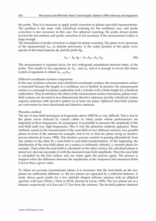
Am = Aa Ap = Aax Apx + Aay Apy (26) The measurement is repeated twice, for two orthogonal orientations between them, of the probe. This results in two equations on Aax and Aay and it is enough to invert this linear system of equations to obtain Aax and Aay. Different coordinates systems comparison In the case of planar cartesian and cylindrical coordinates systems, the measurement surface is truncated because the length of a rectilinear axis is limited. In practice, the measurement surface is a rectangle for planar exploration and a cylinder with a finite height for cylindrical exploration. Thus to minimize the effect of the measurement surface truncation, planar near-field systems are devoted to two-dimensional directive antennas and the cylindrical system requires antennas with directive pattern in at least one plane. Spherical near-field systems are convenient for omni-directional and directive antennas. Phaseless method The use of near-field techniques at frequencies above 100GHz is very difficult. This is due to the phase errors induced by coaxial cables or rotary joints whose performances are degraded at these frequencies. In counterpart, it is possible to measure the amplitude of the near-field until very high frequencies. This is why the phaseless methods appeared. These methods consist in the measurement of the near-field on two different surfaces, two parallel planes in front of the antenna for example, and to try to find the phase using an iterative process (Isernia & Leone, 1994). This iterative process consists in passing alternatively from one surface to the other by a near-field to near-field transformation. At the beginning, the distribution of the near-field phase on a surface is arbitrarily selected, a constant phase for example. Then when the near-field is calculated on the other surface, the calculated phase is preserved, and one associates it with the measured near-field amplitude. Then the near-field is calculated on the first surface and one starts again the process again. The process is stopped when the difference between the amplitudes of the computed and measured fields is lower than a given value. To obtain an accurate reconstructed phase, it is necessary that the near-fields on the two planes are sufficiently different, i.e. the two planes are separated by a sufficient distance. A study shows good results for a low sidelobe shaped reflector antenna with an elliptical aperture with axes 155cm x 52cm at 9GHz (Isernia & Leone, 1995). The two planes are at a distance respectively of 4.2cm and 17.7cm from the antenna. The far-field pattern obtained
from the near to far-field transformation with phaseless method shows agreement with the reference far-field pattern, up to a -25dB level approximately. Fig. 16. Phaseless method with two parallel planes configuration Near-field measurement errors analysis One of the difficulties related to the use of the near-field techniques is the evaluation of the effect on the far field, of the measurement errors intervening on the near-field. A study allows the identification of the error sources, an evaluation of their level and the value of the induced uncertainties on the far-field, in the case of planar near-field measurements (Newell, 1988). About twenty different error sources are identified as probe relative pattern, gain, polarization, or multiple reflections between probe and tested antenna, measurement area truncation, temperature drift… The main error sources on the maximum gains are the multiple reflections between probe and tested antenna, and the power measurement, for a global induced error of 0.23dB. For sidelobe measurement, the main error sources are the multiple reflections between probe and tested antenna, the phase errors, the probe position errors and the probe alignment for a global induced error of 0.53dB on a -30dB sidelobe level. A comparison of the results obtained with four different near-field European ranges shows agreement on the copolar far-field pattern and directivity of a contoured beam antenna (Lemanczyk, 1988).
4.2 Near field applications Electromagnetic antenna diagnosis Antenna diagnosis consists in the detection of defects on an antenna. There are essentially two different electromagnetic diagnosis: reflector antenna diagnosis and array antenna diagnosis.
z1 z2 z
www.intechopen.com

Antenna Measurement 205
the probe. Thus it is necessary to apply probe correction to planar near-field measurements. The problem is the same with cylindrical scanning for the rectilinear axis, and probe correction is also necessary in this case. For spherical scanning, the probe always points toward the test antenna and probe correction is not necessary if the measurement radius is large enough. The formulation of probe correction is simple for planar scanning. The plane wave spectrum of the measurement Am, as definite previously, is the scalar product of the plane wave spectra of the tested antenna Aa and the probe Ap:
Am = Aa Ap = Aax Apx + Aay Apy (26) The measurement is repeated twice, for two orthogonal orientations between them, of the probe. This results in two equations on Aax and Aay and it is enough to invert this linear system of equations to obtain Aax and Aay. Different coordinates systems comparison In the case of planar cartesian and cylindrical coordinates systems, the measurement surface is truncated because the length of a rectilinear axis is limited. In practice, the measurement surface is a rectangle for planar exploration and a cylinder with a finite height for cylindrical exploration. Thus to minimize the effect of the measurement surface truncation, planar near-field systems are devoted to two-dimensional directive antennas and the cylindrical system requires antennas with directive pattern in at least one plane. Spherical near-field systems are convenient for omni-directional and directive antennas. Phaseless method The use of near-field techniques at frequencies above 100GHz is very difficult. This is due to the phase errors induced by coaxial cables or rotary joints whose performances are degraded at these frequencies. In counterpart, it is possible to measure the amplitude of the near-field until very high frequencies. This is why the phaseless methods appeared. These methods consist in the measurement of the near-field on two different surfaces, two parallel planes in front of the antenna for example, and to try to find the phase using an iterative process (Isernia & Leone, 1994). This iterative process consists in passing alternatively from one surface to the other by a near-field to near-field transformation. At the beginning, the distribution of the near-field phase on a surface is arbitrarily selected, a constant phase for example. Then when the near-field is calculated on the other surface, the calculated phase is preserved, and one associates it with the measured near-field amplitude. Then the near-field is calculated on the first surface and one starts again the process again. The process is stopped when the difference between the amplitudes of the computed and measured fields is lower than a given value. To obtain an accurate reconstructed phase, it is necessary that the near-fields on the two planes are sufficiently different, i.e. the two planes are separated by a sufficient distance. A study shows good results for a low sidelobe shaped reflector antenna with an elliptical aperture with axes 155cm x 52cm at 9GHz (Isernia & Leone, 1995). The two planes are at a distance respectively of 4.2cm and 17.7cm from the antenna. The far-field pattern obtained
from the near to far-field transformation with phaseless method shows agreement with the reference far-field pattern, up to a -25dB level approximately. Fig. 16. Phaseless method with two parallel planes configuration Near-field measurement errors analysis One of the difficulties related to the use of the near-field techniques is the evaluation of the effect on the far field, of the measurement errors intervening on the near-field. A study allows the identification of the error sources, an evaluation of their level and the value of the induced uncertainties on the far-field, in the case of planar near-field measurements (Newell, 1988). About twenty different error sources are identified as probe relative pattern, gain, polarization, or multiple reflections between probe and tested antenna, measurement area truncation, temperature drift… The main error sources on the maximum gains are the multiple reflections between probe and tested antenna, and the power measurement, for a global induced error of 0.23dB. For sidelobe measurement, the main error sources are the multiple reflections between probe and tested antenna, the phase errors, the probe position errors and the probe alignment for a global induced error of 0.53dB on a -30dB sidelobe level. A comparison of the results obtained with four different near-field European ranges shows agreement on the copolar far-field pattern and directivity of a contoured beam antenna (Lemanczyk, 1988).
4.2 Near field applications Electromagnetic antenna diagnosis Antenna diagnosis consists in the detection of defects on an antenna. There are essentially two different electromagnetic diagnosis: reflector antenna diagnosis and array antenna diagnosis.
z1 z2 z
www.intechopen.com
Microwave and Millimeter Wave Technologies: Modern UWB antennas and equipment 206
Cylindrical near-field range Spherical near-field range
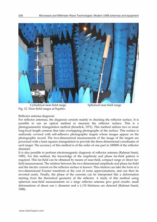
Fig. 12. Near-field ranges at Supélec. Reflector antenna diagnosis For reflector antennas, the diagnosis consists mainly in checking the reflector surface. It is possible to use an optical method to measure the reflector surface. This is a photogrammetric triangulation method (Kenefick, 1971). This method utilizes two or more long-focal length cameras that take overlapping photographs of the surface. This surface is uniformly covered with self-adhesive photographic targets whose images appear on the photographic record. The two-dimensional measurements of the image of the targets are processed with a least squares triangulation to provide the three-dimensional coordinates of each target. The accuracy of this method is of the order of one part in 100000 of the reflector diameter. It is also possible to perform electromagnetic diagnosis of reflector antenna (Rahmat Samii, 1985). For this method, the knowledge of the amplitude and phase far-field pattern is required. This far-field can be obtained by means of near-field, compact range or direct far-field measurement. The relation between the two-dimensional amplitude and phase far-field and the electric current on the reflector surface is known. This relation can take the form of a two-dimensional Fourier transform at the cost of some approximations, and can then be inverted easily. Finally, the phase of the currents can be interpreted like a deformation starting from the theoretical geometry of the reflector. A study of this method using spherical near-field measurements on a large reflector antenna give good results: small deformations of about one diameter and a /10 thickness are detected (Rahmat Samii, 1988).
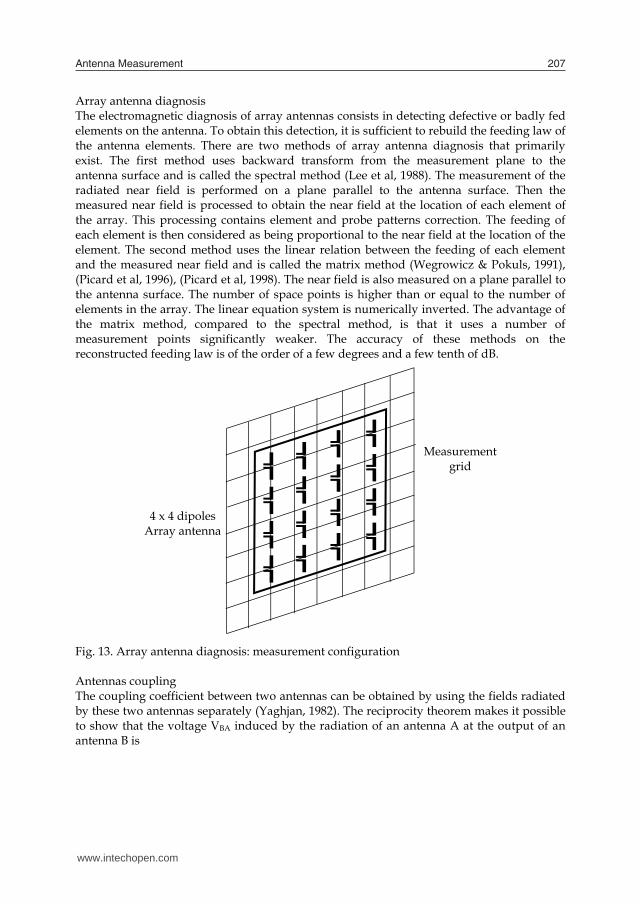
Array antenna diagnosis The electromagnetic diagnosis of array antennas consists in detecting defective or badly fed elements on the antenna. To obtain this detection, it is sufficient to rebuild the feeding law of the antenna elements. There are two methods of array antenna diagnosis that primarily exist. The first method uses backward transform from the measurement plane to the antenna surface and is called the spectral method (Lee et al, 1988). The measurement of the radiated near field is performed on a plane parallel to the antenna surface. Then the measured near field is processed to obtain the near field at the location of each element of the array. This processing contains element and probe patterns correction. The feeding of each element is then considered as being proportional to the near field at the location of the element. The second method uses the linear relation between the feeding of each element and the measured near field and is called the matrix method (Wegrowicz & Pokuls, 1991), (Picard et al, 1996), (Picard et al, 1998). The near field is also measured on a plane parallel to the antenna surface. The number of space points is higher than or equal to the number of elements in the array. The linear equation system is numerically inverted. The advantage of the matrix method, compared to the spectral method, is that it uses a number of measurement points significantly weaker. The accuracy of these methods on the reconstructed feeding law is of the order of a few degrees and a few tenth of dB. Fig. 13. Array antenna diagnosis: measurement configuration Antennas coupling The coupling coefficient between two antennas can be obtained by using the fields radiated by these two antennas separately (Yaghjan, 1982). The reciprocity theorem makes it possible to show that the voltage VBA induced by the radiation of an antenna A at the output of an antenna B is
Measurement grid
4 x 4 dipoles Array antenna
www.intechopen.com
Antenna Measurement 207
Cylindrical near-field range Spherical near-field range
Fig. 12. Near-field ranges at Supélec. Reflector antenna diagnosis For reflector antennas, the diagnosis consists mainly in checking the reflector surface. It is possible to use an optical method to measure the reflector surface. This is a photogrammetric triangulation method (Kenefick, 1971). This method utilizes two or more long-focal length cameras that take overlapping photographs of the surface. This surface is uniformly covered with self-adhesive photographic targets whose images appear on the photographic record. The two-dimensional measurements of the image of the targets are processed with a least squares triangulation to provide the three-dimensional coordinates of each target. The accuracy of this method is of the order of one part in 100000 of the reflector diameter. It is also possible to perform electromagnetic diagnosis of reflector antenna (Rahmat Samii, 1985). For this method, the knowledge of the amplitude and phase far-field pattern is required. This far-field can be obtained by means of near-field, compact range or direct far-field measurement. The relation between the two-dimensional amplitude and phase far-field and the electric current on the reflector surface is known. This relation can take the form of a two-dimensional Fourier transform at the cost of some approximations, and can then be inverted easily. Finally, the phase of the currents can be interpreted like a deformation starting from the theoretical geometry of the reflector. A study of this method using spherical near-field measurements on a large reflector antenna give good results: small deformations of about one diameter and a /10 thickness are detected (Rahmat Samii, 1988).
Array antenna diagnosis The electromagnetic diagnosis of array antennas consists in detecting defective or badly fed elements on the antenna. To obtain this detection, it is sufficient to rebuild the feeding law of the antenna elements. There are two methods of array antenna diagnosis that primarily exist. The first method uses backward transform from the measurement plane to the antenna surface and is called the spectral method (Lee et al, 1988). The measurement of the radiated near field is performed on a plane parallel to the antenna surface. Then the measured near field is processed to obtain the near field at the location of each element of the array. This processing contains element and probe patterns correction. The feeding of each element is then considered as being proportional to the near field at the location of the element. The second method uses the linear relation between the feeding of each element and the measured near field and is called the matrix method (Wegrowicz & Pokuls, 1991), (Picard et al, 1996), (Picard et al, 1998). The near field is also measured on a plane parallel to the antenna surface. The number of space points is higher than or equal to the number of elements in the array. The linear equation system is numerically inverted. The advantage of the matrix method, compared to the spectral method, is that it uses a number of measurement points significantly weaker. The accuracy of these methods on the reconstructed feeding law is of the order of a few degrees and a few tenth of dB. Fig. 13. Array antenna diagnosis: measurement configuration Antennas coupling The coupling coefficient between two antennas can be obtained by using the fields radiated by these two antennas separately (Yaghjan, 1982). The reciprocity theorem makes it possible to show that the voltage VBA induced by the radiation of an antenna A at the output of an antenna B is
Measurement grid
4 x 4 dipoles Array antenna
www.intechopen.com

Microwave and Millimeter Wave Technologies: Modern UWB antennas and equipment 208
VBA = - S
[EaxHb + HaxEb] n dS (27)
S is a close surface surrounding the antenna B, n is the normal vector to S with the outside orientation, Ea, Ha electric and magnetic fields radiated by the antenna A, Eb,Hb electric and magnetic fields radiated by the antenna A for the emission mode with unit input current, Fig. 14. The two antennas system for coupling evaluation The advantage of this method is that it can predict, by calculation, the coupling between the two antennas for any relative position, only by means of their separate radiated near-fields measurements. Determination of the safety perimeter of base station antennas An application of the cylindrical near-field to near-field transformations is the determination of the base station antennas safety perimeter. The electric and magnetic near-fields level can be evaluated from the near-field measurements and from the power accepted by the antenna. The comparison of this level with the ICNIRP reference level allows the determination of the safety perimeter (Ziyyat et al, 2001), (ICNIRP, 1998). The accuracy obtained by this method is within a few percent on the calculated near-field. Rapid near-field assessment system The near-field measurement of a large antenna requires a considerable number of measurement points. Computers’ computing power has increased regularly and was multiplied by approximately 100000 between 1981 and 2006. The result is from it that the duration of the far-field calculation decreases regularly and is no longer a problem. On the other hand the duration of measurement can be very important. This is due to the slowness of mechanical displacements. The replacement of the mechanical displacement of the probe by the electronic scanning of a probes array makes it possible to accelerate considerably the measurement rate and to reduce the measurement duration (Picard et al., 1992), (Picard et al, 1998).
Antenna A Antenna B
VBA
S Antenna B
IA = 1
n
Fig. 15. Rapid near-field range at Supélec and principle of rapid near-field assessment systems
5. Electromagnetic field measurement method
The measurement of the radiation of the antennas is indissociable from the measurement of high frequency electromagnetic field. Primarily four different methods for high frequency electromagnetic field measurement exist. These methods differ primarily by the type of connection between the probe and the receiver, this connection could possibly be the cause of many disturbances. The first method is the simplest one. It consists in using of a small dipole probe connected to a receiver with a coaxial line. In order to limit the parasitic effects of the line on the measurement signal, a balun is placed between the line and the dipole. This method makes it possible the measurement of the local value of one component of the electric or magnetic field. Fig. 17. Measurement of the electric and magnetic field with a dipole probe
Vertical rectilinear array of bipolarized probes with
electronic scanning
Tested antenna on turning table
+ + + + + + + + + + + + + + + + + + +
Bifilar line Balun Coaxial line Two-wire line Balun Coaxial line
www.intechopen.com

Antenna Measurement 209
VBA = - S
[EaxHb + HaxEb] n dS (27)
S is a close surface surrounding the antenna B, n is the normal vector to S with the outside orientation, Ea, Ha electric and magnetic fields radiated by the antenna A, Eb,Hb electric and magnetic fields radiated by the antenna A for the emission mode with unit input current, Fig. 14. The two antennas system for coupling evaluation The advantage of this method is that it can predict, by calculation, the coupling between the two antennas for any relative position, only by means of their separate radiated near-fields measurements. Determination of the safety perimeter of base station antennas An application of the cylindrical near-field to near-field transformations is the determination of the base station antennas safety perimeter. The electric and magnetic near-fields level can be evaluated from the near-field measurements and from the power accepted by the antenna. The comparison of this level with the ICNIRP reference level allows the determination of the safety perimeter (Ziyyat et al, 2001), (ICNIRP, 1998). The accuracy obtained by this method is within a few percent on the calculated near-field. Rapid near-field assessment system The near-field measurement of a large antenna requires a considerable number of measurement points. Computers’ computing power has increased regularly and was multiplied by approximately 100000 between 1981 and 2006. The result is from it that the duration of the far-field calculation decreases regularly and is no longer a problem. On the other hand the duration of measurement can be very important. This is due to the slowness of mechanical displacements. The replacement of the mechanical displacement of the probe by the electronic scanning of a probes array makes it possible to accelerate considerably the measurement rate and to reduce the measurement duration (Picard et al., 1992), (Picard et al, 1998).
Antenna A Antenna B
VBA
S Antenna B
IA = 1
n
Fig. 15. Rapid near-field range at Supélec and principle of rapid near-field assessment systems
5. Electromagnetic field measurement method
The measurement of the radiation of the antennas is indissociable from the measurement of high frequency electromagnetic field. Primarily four different methods for high frequency electromagnetic field measurement exist. These methods differ primarily by the type of connection between the probe and the receiver, this connection could possibly be the cause of many disturbances. The first method is the simplest one. It consists in using of a small dipole probe connected to a receiver with a coaxial line. In order to limit the parasitic effects of the line on the measurement signal, a balun is placed between the line and the dipole. This method makes it possible the measurement of the local value of one component of the electric or magnetic field. Fig. 17. Measurement of the electric and magnetic field with a dipole probe
Vertical rectilinear array of bipolarized probes with
electronic scanning
Tested antenna on turning table
+ + + + + + + + + + + + + + + + + + +
Bifilar line Balun Coaxial line Two-wire line Balun Coaxial line
www.intechopen.com
Microwave and Millimeter Wave Technologies: Modern UWB antennas and equipment 210
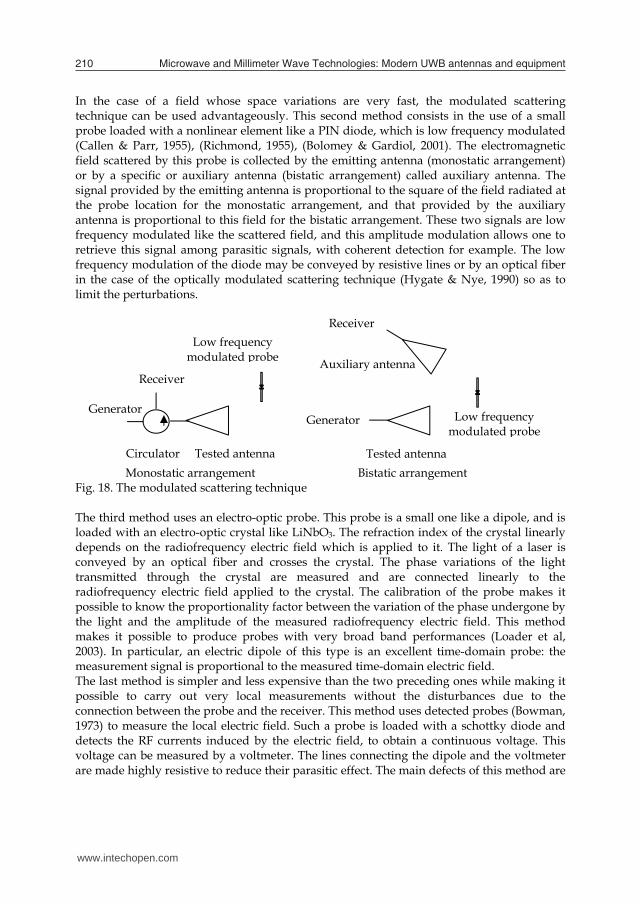
In the case of a field whose space variations are very fast, the modulated scattering technique can be used advantageously. This second method consists in the use of a small probe loaded with a nonlinear element like a PIN diode, which is low frequency modulated (Callen & Parr, 1955), (Richmond, 1955), (Bolomey & Gardiol, 2001). The electromagnetic field scattered by this probe is collected by the emitting antenna (monostatic arrangement) or by a specific or auxiliary antenna (bistatic arrangement) called auxiliary antenna. The signal provided by the emitting antenna is proportional to the square of the field radiated at the probe location for the monostatic arrangement, and that provided by the auxiliary antenna is proportional to this field for the bistatic arrangement. These two signals are low frequency modulated like the scattered field, and this amplitude modulation allows one to retrieve this signal among parasitic signals, with coherent detection for example. The low frequency modulation of the diode may be conveyed by resistive lines or by an optical fiber in the case of the optically modulated scattering technique (Hygate & Nye, 1990) so as to limit the perturbations.
Monostatic arrangement Bistatic arrangement Fig. 18. The modulated scattering technique The third method uses an electro-optic probe. This probe is a small one like a dipole, and is loaded with an electro-optic crystal like LiNbO3. The refraction index of the crystal linearly depends on the radiofrequency electric field which is applied to it. The light of a laser is conveyed by an optical fiber and crosses the crystal. The phase variations of the light transmitted through the crystal are measured and are connected linearly to the radiofrequency electric field applied to the crystal. The calibration of the probe makes it possible to know the proportionality factor between the variation of the phase undergone by the light and the amplitude of the measured radiofrequency electric field. This method makes it possible to produce probes with very broad band performances (Loader et al, 2003). In particular, an electric dipole of this type is an excellent time-domain probe: the measurement signal is proportional to the measured time-domain electric field. The last method is simpler and less expensive than the two preceding ones while making it possible to carry out very local measurements without the disturbances due to the connection between the probe and the receiver. This method uses detected probes (Bowman, 1973) to measure the local electric field. Such a probe is loaded with a schottky diode and detects the RF currents induced by the electric field, to obtain a continuous voltage. This voltage can be measured by a voltmeter. The lines connecting the dipole and the voltmeter are made highly resistive to reduce their parasitic effect. The main defects of this method are
Low frequency modulated probe
Receiver
Generator
Auxiliary antenna
Tested antenna Circulator Tested antenna
Generator
Receiver
Low frequency modulated probe
its poor sensitivity and that it provides only the amplitude of the measured field. If the knowledge of the phase is necessary for the application, it must be obtained by means of phaseless methods. Fig. 19. Electro-optic dipole probe Fig. 20. Detected probe
6. Instrumentation
The instrumentation used for antenna measurements depends on the temporal mode used: time domain or frequency domain. Network or spectrum analyzer and frequency synthetizer are used for frequency domain measurements. Real time or sampling oscilloscope and pulse generator are used for time domain measurements. Frequency domain antenna measurements The system of emission-reception the most used for antenna measurements is the vector network analyzer. It allows the measurement of transmission coefficients and it supplies the phase. Its intermediary frequency bandwidth can reach 1MHz, i.e. it allows very high speed measurements, and its dynamic can reach 140dB. It can have several ways of measurement so as to be able to measure simultaneously direct and cross polarizations. Its maximum frequency bandwidth of operation is 30kHz to 1000GHz (with several models). It is also possible to use a scalar network analyzer or a spectrum analyzer coupled to a frequency synthetizer when the measurement of the phase is not necessary as for far-field for example. Time domain antenna measurements Antenna measurements in the time domain are less frequent than in the frequency domain. The measurement signal is delivered by a pulse generator. Certain characteristics of the pulse can be adjusted: the rise and fall times, the duration, the repetition rate and the
Electric dipole
Electro-optic crystal
Optical fiber
Low frequency amplifier
Resistive line Voltmeter Resistive line
Low frequency amplifier
Voltmeter
www.intechopen.com

Antenna Measurement 211
In the case of a field whose space variations are very fast, the modulated scattering technique can be used advantageously. This second method consists in the use of a small probe loaded with a nonlinear element like a PIN diode, which is low frequency modulated (Callen & Parr, 1955), (Richmond, 1955), (Bolomey & Gardiol, 2001). The electromagnetic field scattered by this probe is collected by the emitting antenna (monostatic arrangement) or by a specific or auxiliary antenna (bistatic arrangement) called auxiliary antenna. The signal provided by the emitting antenna is proportional to the square of the field radiated at the probe location for the monostatic arrangement, and that provided by the auxiliary antenna is proportional to this field for the bistatic arrangement. These two signals are low frequency modulated like the scattered field, and this amplitude modulation allows one to retrieve this signal among parasitic signals, with coherent detection for example. The low frequency modulation of the diode may be conveyed by resistive lines or by an optical fiber in the case of the optically modulated scattering technique (Hygate & Nye, 1990) so as to limit the perturbations.
Monostatic arrangement Bistatic arrangement Fig. 18. The modulated scattering technique The third method uses an electro-optic probe. This probe is a small one like a dipole, and is loaded with an electro-optic crystal like LiNbO3. The refraction index of the crystal linearly depends on the radiofrequency electric field which is applied to it. The light of a laser is conveyed by an optical fiber and crosses the crystal. The phase variations of the light transmitted through the crystal are measured and are connected linearly to the radiofrequency electric field applied to the crystal. The calibration of the probe makes it possible to know the proportionality factor between the variation of the phase undergone by the light and the amplitude of the measured radiofrequency electric field. This method makes it possible to produce probes with very broad band performances (Loader et al, 2003). In particular, an electric dipole of this type is an excellent time-domain probe: the measurement signal is proportional to the measured time-domain electric field. The last method is simpler and less expensive than the two preceding ones while making it possible to carry out very local measurements without the disturbances due to the connection between the probe and the receiver. This method uses detected probes (Bowman, 1973) to measure the local electric field. Such a probe is loaded with a schottky diode and detects the RF currents induced by the electric field, to obtain a continuous voltage. This voltage can be measured by a voltmeter. The lines connecting the dipole and the voltmeter are made highly resistive to reduce their parasitic effect. The main defects of this method are
Low frequency modulated probe
Receiver
Generator
Auxiliary antenna
Tested antenna Circulator Tested antenna
Generator
Receiver
Low frequency modulated probe
its poor sensitivity and that it provides only the amplitude of the measured field. If the knowledge of the phase is necessary for the application, it must be obtained by means of phaseless methods. Fig. 19. Electro-optic dipole probe Fig. 20. Detected probe
6. Instrumentation
The instrumentation used for antenna measurements depends on the temporal mode used: time domain or frequency domain. Network or spectrum analyzer and frequency synthetizer are used for frequency domain measurements. Real time or sampling oscilloscope and pulse generator are used for time domain measurements. Frequency domain antenna measurements The system of emission-reception the most used for antenna measurements is the vector network analyzer. It allows the measurement of transmission coefficients and it supplies the phase. Its intermediary frequency bandwidth can reach 1MHz, i.e. it allows very high speed measurements, and its dynamic can reach 140dB. It can have several ways of measurement so as to be able to measure simultaneously direct and cross polarizations. Its maximum frequency bandwidth of operation is 30kHz to 1000GHz (with several models). It is also possible to use a scalar network analyzer or a spectrum analyzer coupled to a frequency synthetizer when the measurement of the phase is not necessary as for far-field for example. Time domain antenna measurements Antenna measurements in the time domain are less frequent than in the frequency domain. The measurement signal is delivered by a pulse generator. Certain characteristics of the pulse can be adjusted: the rise and fall times, the duration, the repetition rate and the
Electric dipole
Electro-optic crystal
Optical fiber
Low frequency amplifier
Resistive line Voltmeter Resistive line
Low frequency amplifier
Voltmeter
www.intechopen.com
Microwave and Millimeter Wave Technologies: Modern UWB antennas and equipment 212
amplitude. The receiver is a fast oscilloscope. The real time oscilloscope acquires the measured time response in one step, but its sensitivity is limited and it is very expensive. The sampling oscilloscope requires numerous repetitions of the measurement signal to acquire its time response, but its sensitivity is better and its price is lower than those of the real time oscilloscope. In 2009, the maximum frequency of operation for real time oscilloscope is 20GHz and 75GHz for sample oscilloscope. Probe Direct far-field measurements use a source antenna. The dimensions of this source antenna are limited by the distance between this antenna and the tested antenna. A large source antenna increases the measurement signal and decreases the parasitic reflections. The measured polarization is the one of the source antenna. Near-field measurements can use several types of probe: open-ended circular or rectangular metallic waveguide and electric dipole for narrow band operation (half a octave) and ridged waveguide for broad band operation (a decade).
7. Conclusion
Currently it is possible to measure all the characteristics of an antenna with a good accuracy. Far-field ranges do not have a very good accuracy, due to parasitic reflections for the outdoor ranges and because of the limited distance between the source antenna and the tested antenna for the indoor ranges. The compact range allows one to obtain a direct far-field cut in a relatively short time. The near-field techniques are the most accurate and the most convenient for global antenna radiation testing. Their main defect is the duration of the measurement which rises from the large number of necessary space points. Rapid near-field measurement systems allow one to solve this problem, but the accuracy is less good, and the frequency bandwidth is limited. Progress is necessary in this field. Research relates to the rise in frequency, with for solutions the hologram compact antenna test range and the phaseless methods. The hologram compact antenna test range must improve their accuracy while the phaseless methods must improve their reliability. Electromagnetic diagnosis of antenna must be optimized on a case-by-case basis.
8. References
Ashkenazy, J. et al. (1985). Radiometric measurement of antenna efficiency, Electronics letters, Vol.21, N°3, January 1985, pp.111-112, ISSN 0013-5194
Bolomey, J. C. & Gardiol, F.E. (2001). Engineering applications of the modulated scatterer technique, Artech House Inc, ISBN 1-58053-147-4, 685 Canton Street, Norwood, MA 02062 USA
Bowman, R. R. (1973). Some recent developments in the characterization and measurement of hazardous electromagnetic fields, International Symposium, Warsaw, October 1973, pp217-227
Callen, A. L. & Parr, J. C. (1955). A new perturbation method for measuring microwave fields in free space, IEE(GB), n°102, 1955, p.836
Hygate, G. & Nye J. F. (1990). Measurement microwave fields directly with an optically modulated scatterer, Measurement Science and Technology’s, 1990, pp.703-709, ISSN 0957-0233
Hirvonen, T. et al. (1997). A compact antenna test range based on a hologram, IEEE Transactions on Antennas and Propagation, Vol.AP45, N°8, August 1997, pp.1270-1276, ISSN 0018-926X
ICNIRP, (1998). Guide pour l’établissement de limites d’exposition aux champs électriques, magnétiques et électromagnétiques, Health Physics Society, Vol.74, n°4, 1998, pp.494-522, ISSN 0017-9078
Isernia, T. & Leone, G. (1994). Phaseless near-field techniques : formulation of the problem and field properties, Journal of electromagnetic waves and applications, Vol.8, N°1, 1995, pp.267-284, ISSN 0920-5071
Isernia, T. & Leone, G. (1995). Numerical and experimental validation of a phaseless planar near-field technique, Journal of electromagnetic waves and applications, Vol.9, N°7, 1994, pp.871-888, ISSN 0920-5071
Johnson, R. C. et al. (1969). Compact range techniques and measurements, IEEE Transactions on Antennas and Propagation, Vol.AP17, N°5, September 1969, 568-576, ISSN 0018-926X
Johnson, R. C. et al. (1973). Determination of far-field antennas patterns from near-field measurements, Proceeding of the IEEE, Vol.61, N°12, December 1973, pp.1668-1694, ISSN 0018-9219
Kenefick, J. F. (1971). Ultra-precise analytics, Photogrammetry Engineering, Vol.37, 1971, pp.1167-1187, ISSN 0031-8671
Kummer, W. & Gillepsie, E. (1978). Antenna measurement – 1978, Proceedings of the IEEE, Vol.66, N°4, April 1978, 483-507, ISSN 0018-9219
Lee, J.J. et al. (1988). Near-field probe used as a diagnostic tool to locate defective elements in an array antenna, IEEE Transactions on Antennas and Propagation, Vol.AP36, n°6, June 1988, ISSN 0018-926X
Lemanczyk, H. (1988). Comparison of near-field range results, IEEE Transactions on Antennas and Propagation, VolAP36, n°6, June 1988, pp.845-851, ISSN 0018-926X
Loader, B. G. et al. (2003). An optical electric field probe for specific absorption rate measurements, The 15th International Zurich Symposium, 2003, pp.57-60
Newell, A. C. (1988). Error analysis techniques for planar near-field measurements, IEEE Transactions on Antennas and Propagation, VolAP36, n°6, June 1988, pp.754-768, ISSN 0018-926X
Picard, D. et al. (1992). Real time analyser of antenna near-field distribution, 22nd European Microwave Conference, Vol..1, pp.509-514, Espoo, Finland, 24-27 August 1992
Picard, D. et al. (1996). Reconstruction de la loi d'alimentation des antennes réseau à partir d'une mesure de champ proche par la méthode matricielle, Jina 1996, Novembre 1996, Nice
Picard, D. et al. (1998). Broadband and low interaction rapid cylindrical facility, PIERS 1998, Nantes, France, July 1998, pp.13-17
Picard, D. & Gattoufi, L. (1998). Diagnostic d’antennes réseau par des méthodes matricielles, Revue de l’Electricité et de l’Electronique, n°9, Octobre 1998
www.intechopen.com

Antenna Measurement 213
amplitude. The receiver is a fast oscilloscope. The real time oscilloscope acquires the measured time response in one step, but its sensitivity is limited and it is very expensive. The sampling oscilloscope requires numerous repetitions of the measurement signal to acquire its time response, but its sensitivity is better and its price is lower than those of the real time oscilloscope. In 2009, the maximum frequency of operation for real time oscilloscope is 20GHz and 75GHz for sample oscilloscope. Probe Direct far-field measurements use a source antenna. The dimensions of this source antenna are limited by the distance between this antenna and the tested antenna. A large source antenna increases the measurement signal and decreases the parasitic reflections. The measured polarization is the one of the source antenna. Near-field measurements can use several types of probe: open-ended circular or rectangular metallic waveguide and electric dipole for narrow band operation (half a octave) and ridged waveguide for broad band operation (a decade).
7. Conclusion
Currently it is possible to measure all the characteristics of an antenna with a good accuracy. Far-field ranges do not have a very good accuracy, due to parasitic reflections for the outdoor ranges and because of the limited distance between the source antenna and the tested antenna for the indoor ranges. The compact range allows one to obtain a direct far-field cut in a relatively short time. The near-field techniques are the most accurate and the most convenient for global antenna radiation testing. Their main defect is the duration of the measurement which rises from the large number of necessary space points. Rapid near-field measurement systems allow one to solve this problem, but the accuracy is less good, and the frequency bandwidth is limited. Progress is necessary in this field. Research relates to the rise in frequency, with for solutions the hologram compact antenna test range and the phaseless methods. The hologram compact antenna test range must improve their accuracy while the phaseless methods must improve their reliability. Electromagnetic diagnosis of antenna must be optimized on a case-by-case basis.
8. References
Ashkenazy, J. et al. (1985). Radiometric measurement of antenna efficiency, Electronics letters, Vol.21, N°3, January 1985, pp.111-112, ISSN 0013-5194
Bolomey, J. C. & Gardiol, F.E. (2001). Engineering applications of the modulated scatterer technique, Artech House Inc, ISBN 1-58053-147-4, 685 Canton Street, Norwood, MA 02062 USA
Bowman, R. R. (1973). Some recent developments in the characterization and measurement of hazardous electromagnetic fields, International Symposium, Warsaw, October 1973, pp217-227
Callen, A. L. & Parr, J. C. (1955). A new perturbation method for measuring microwave fields in free space, IEE(GB), n°102, 1955, p.836
Hygate, G. & Nye J. F. (1990). Measurement microwave fields directly with an optically modulated scatterer, Measurement Science and Technology’s, 1990, pp.703-709, ISSN 0957-0233
Hirvonen, T. et al. (1997). A compact antenna test range based on a hologram, IEEE Transactions on Antennas and Propagation, Vol.AP45, N°8, August 1997, pp.1270-1276, ISSN 0018-926X
ICNIRP, (1998). Guide pour l’établissement de limites d’exposition aux champs électriques, magnétiques et électromagnétiques, Health Physics Society, Vol.74, n°4, 1998, pp.494-522, ISSN 0017-9078
Isernia, T. & Leone, G. (1994). Phaseless near-field techniques : formulation of the problem and field properties, Journal of electromagnetic waves and applications, Vol.8, N°1, 1995, pp.267-284, ISSN 0920-5071
Isernia, T. & Leone, G. (1995). Numerical and experimental validation of a phaseless planar near-field technique, Journal of electromagnetic waves and applications, Vol.9, N°7, 1994, pp.871-888, ISSN 0920-5071
Johnson, R. C. et al. (1969). Compact range techniques and measurements, IEEE Transactions on Antennas and Propagation, Vol.AP17, N°5, September 1969, 568-576, ISSN 0018-926X
Johnson, R. C. et al. (1973). Determination of far-field antennas patterns from near-field measurements, Proceeding of the IEEE, Vol.61, N°12, December 1973, pp.1668-1694, ISSN 0018-9219
Kenefick, J. F. (1971). Ultra-precise analytics, Photogrammetry Engineering, Vol.37, 1971, pp.1167-1187, ISSN 0031-8671
Kummer, W. & Gillepsie, E. (1978). Antenna measurement – 1978, Proceedings of the IEEE, Vol.66, N°4, April 1978, 483-507, ISSN 0018-9219
Lee, J.J. et al. (1988). Near-field probe used as a diagnostic tool to locate defective elements in an array antenna, IEEE Transactions on Antennas and Propagation, Vol.AP36, n°6, June 1988, ISSN 0018-926X
Lemanczyk, H. (1988). Comparison of near-field range results, IEEE Transactions on Antennas and Propagation, VolAP36, n°6, June 1988, pp.845-851, ISSN 0018-926X
Loader, B. G. et al. (2003). An optical electric field probe for specific absorption rate measurements, The 15th International Zurich Symposium, 2003, pp.57-60
Newell, A. C. (1988). Error analysis techniques for planar near-field measurements, IEEE Transactions on Antennas and Propagation, VolAP36, n°6, June 1988, pp.754-768, ISSN 0018-926X
Picard, D. et al. (1992). Real time analyser of antenna near-field distribution, 22nd European Microwave Conference, Vol..1, pp.509-514, Espoo, Finland, 24-27 August 1992
Picard, D. et al. (1996). Reconstruction de la loi d'alimentation des antennes réseau à partir d'une mesure de champ proche par la méthode matricielle, Jina 1996, Novembre 1996, Nice
Picard, D. et al. (1998). Broadband and low interaction rapid cylindrical facility, PIERS 1998, Nantes, France, July 1998, pp.13-17
Picard, D. & Gattoufi, L. (1998). Diagnostic d’antennes réseau par des méthodes matricielles, Revue de l’Electricité et de l’Electronique, n°9, Octobre 1998
www.intechopen.com

Microwave and Millimeter Wave Technologies: Modern UWB antennas and equipment 214
Pozar, D. & Kaufman, B. (1988). Comparison of three methods for the measurement of printed antennas efficiency, IEEE Transactions on Antennas and Propagation, Vol.AP36, N°1, January 1988, 136-139, ISSN 0018-926X
Rahmat Samii, Y. (1985). Microwave holography of large reflector antennas simulation algorithms, IEEE Transaction on Antennas and Propagation, Vol.AP33, N°11, November 1985, ISSN 0018-926X
Rahmat Samii, Y. (1988). Application of spherical near-field measurements to microwave holographic diagnosis of antennas, IEEE Transaction on Antennas and Propagation, VolAP36, n°6, June 1988, ISSN 0018-926X
Richmond, J. H. (1955). A modulated scattering technique for measurement of field distribution, IRE Transactions on Microwave theory and technique, Vol.3, 1955, pp.13-17
Slater, D. (1991). Near-field antenna measurements, Artech House Inc, ISBN 0-89006-361-3, 685 Canton Street, Norwood, MA 02062 USA
Wegrowicz, L.A. & Pokuls, R.. (1991). Inverse problem approach to array diagnostics, IEEE AP-S International Symposium, Ontario, Canada, pp.1292-1295, 24-28 June 1991
Yaghjan, A.D. (1982). Efficient computation of antenna coupling and fields within the near-field region, IEEE Transactions on antennas and Propagation, Vol. AP30, n°1, January 1982, pp113-127, ISSN 0018-926X
Yaghjian, A. (1986). An overview of near-field antenna measurements, IEEE Transactions on Antennas and Propagation, Vol.AP34, N°1, January 1986, 30-45, ISSN 0018-926X
Ziyyat, A. et al. (2001). Prediction of BTS antennas safety perimeter from near-field to near-field transformation : an experimental validation, AMTA’2001 Symposium, Denver, Colorado, USA, October 2001
www.intechopen.com

Microwave and Millimeter Wave Technologies Modern UWBantennas and equipmentEdited by Igor Mini
ISBN 978-953-7619-67-1Hard cover, 488 pagesPublisher InTechPublished online 01, March, 2010Published in print edition March, 2010
InTech EuropeUniversity Campus STeP Ri Slavka Krautzeka 83/A 51000 Rijeka, Croatia Phone: +385 (51) 770 447 Fax: +385 (51) 686 166www.intechopen.com
InTech ChinaUnit 405, Office Block, Hotel Equatorial Shanghai No.65, Yan An Road (West), Shanghai, 200040, China
Phone: +86-21-62489820 Fax: +86-21-62489821
How to referenceIn order to correctly reference this scholarly work, feel free to copy and paste the following:
Dominique Picard (2010). Antenna Measurement, Microwave and Millimeter Wave Technologies Modern UWBantennas and equipment, Igor Mini (Ed.), ISBN: 978-953-7619-67-1, InTech, Available from:http://www.intechopen.com/books/microwave-and-millimeter-wave-technologies-modern-uwb-antennas-and-equipment/antenna-measurement

© 2010 The Author(s). Licensee IntechOpen. This chapter is distributedunder the terms of the Creative Commons Attribution-NonCommercial-ShareAlike-3.0 License, which permits use, distribution and reproduction fornon-commercial purposes, provided the original is properly cited andderivative works building on this content are distributed under the samelicense.