dot/faa/ar-03/49 computational fluid dynamics code for

DOT/FAA/AR-03/49 Office of Aviation Research Washington, D.C. 20591

Computational Fluid Dynamics Code for Smoke Transport During an Aircraft Cargo Compartment Fire: Transport Solver, Graphical User Interface, and Preliminary Baseline Validation October 2003 Final Report This document is available to the U.S. public through the National Technical Information Service (NTIS), Springfield, Virginia 22161.

U.S. Department of Transportation Federal Aviation Administration

NOTICE

This document is disseminated under the sponsorship of the U.S. Department of Transportation in the interest of information exchange. The United States Government assumes no liability for the contents or use thereof. The United States Government does not endorse products or manufacturers. Trade or manufacturer's names appear herein solely because they are considered essential to the objective of this report. This document does not constitute FAA certification policy. Consult your local FAA aircraft certification office as to its use. This report is available at the Federal Aviation Administration William J. Hughes Technical Center's Full-Text Technical Reports page: actlibrary.tc.faa.gov in Adobe Acrobat portable document format (PDF).

Technical Report Documentation Page 1. Report No. DOT/FAA/AR-03/49

2. Government Accession No. 3. Recipient's Catalog No.

4. Title and Subtitle

COMPUTATIONAL FLUID DYNAMICS CODE FOR SMOKE TRANSPORT DURING AN AIRCRAFT CARGO COMPARTMENT FIRE: TRANSPORT

5. Report Date

October 2003

SOLVER, GRAPHICAL USER INTERFACE, AND PRELIMINARY BASELINE VALIDATION

6. Performing Organization Code

7. Author(s)

Jill Suo-Anttila, Walt Gill, Carlos Gallegos, and James Nelsen 8. Performing Organization Report No.

9. Performing Organization Name and Address

Fire Science and Technology Department Sandia National Laboratories

10. Work Unit No. (TRAIS)

P.O. Box 5800 MS 1135 Albuquerque, NM 87185

11. Contract or Grant No.

12. Sponsoring Agency Name and Address

U.S. Department of Transportation Federal Aviation Administration

13. Type of Report and Period Covered

Final Report

Office of Aviation Research Washington, DC 20591

14. Sponsoring Agency Code

ANM-110 15. Supplementary Notes

The FAA William J. Hughes Technical Center Technical Monitor was Mr. David Blake. 16. Abstract

Current regulations require that aircraft cargo compartment smoke detectors alarm within 1 minute of the start of a fire and at a time before the fire has substantially decreased the structural integrity of the airplane. Presently, in-flight tests, which can be costly and time consuming, are required to demonstrate compliance with the regulations. A physics-based Computational Fluid Dynamics (CFD) tool, which couples heat, mass, and momentum transfer, has been developed to decrease the time and cost of the certification process by reducing the total number of both in-flight and ground experiments. The tool provides information on smoke transport in cargo compartments under various conditions, therefore allowing optimal experiments to be designed. The CFD-based smoke transport model has the potential to enhance the certification process by determining worst-case locations for fires, optimum placement of fire detector sensors within the cargo compartment, and sensor alarm levels needed to achieve detection within the required certification time. The model is fast running, allowing for simulation of numerous fire scenarios in a short period of time. In addition, the model is user-friendly since it will potentially be used by airframers and airlines that are not expected to be experts in CFD. Following verification of this CFD code, full-scale experiments have been initiated to aid in the validation of the code and gauge the reliability of using such an approach to increase the efficiency of the aircraft fire detection system certification process. This document includes a description of the CFD model, the pre- and postprocessor, and the inital baseline validation results.

17. Key Words

Smoke, Detection, Transport, Cargo compartment, CFD modeling

18. Distribution Statement

This document is available to the public through the National Technical Information Service (NTIS) Springfield, Virginia 22161.

19. Security Classif. (of this report)

Unclassified

20. Security Classif. (of this page)

Unclassified

21. No. of Pages

50 22. Price

Form DOT F1700.7 (8-72) Reproduction of completed page authorized

ACKNOWLEDGEMENTS

Sandia National Laboratories is a multiprogram laboratory operated by Sandia Corporation, a Lockheed-Martin Company, for the United States Department of Energy under Contract DE-AC04-94AL85000. This project was conducted in collaboration with the Federal Aviation Administration (FAA) William J. Hughes Technical Center, Atlantic City International Airport, NJ, and NASA Glenn Research Center. The work presented in this report was performed by a team of individuals at Sandia National Laboratories and the FAA Technical Center. Contributions by the following individuals are acknowledged. Sandia National Laboratories • Stefan Domino, Carlos Gallegos, and Jim Nelsen—Code Development • Walt Gill—Experimental • Jill Suo-Anttila—Program Management, Experimental, CFD Analysis • Lou Gritzo—Program Management, Technical Consultant FAA William J. Hughes Technical Center • David Blake—Program Management, Full-Scale Validation Experiments • Robert Filipczak and Louise Speitel—Cone Calorimeter Experiments

iii/iv

TABLE OF CONTENTS Page EXECUTIVE SUMMARY ix BACKGROUND 1

INTRODUCTION 1

TRANSPORT SOLVER 2

Mathematical Formulation 3 Turbulence Modeling 4 Clutter Modeling for Densely Packed Compartments 7 Numerical Formulation 9 Body-Fitted Grid Transformation 11 Solution Algorithm 12 Summary of Transport Solver 13

GRAPHICAL USER INTERFACE 13

Development Platform and Tools 13 Software Design 14 Preprocessor 14 Coupling to the Analysis Module 16 Postprocessor 16 Summary of Graphical User Interface 17

BASELINE VALIDATION 17

Selected Validation Metrics 17 Experimental Description 17 Computational Model Description 19

CEILING TEMPERATURES 21

Experimental Temperatures 21 Computational Temperatures 23 Comparison of Temperatures 26

LIGHT TRANSMISSION 30

Experimental Light Transmission 30 Computational Light Transmission 31 Comparison of Light Transmission 31

v

GAS CONCENTRATIONS 35

Experimental Gas Concentrations 35 Computational Gas Concentrations 37 Comparison of Gas Concentrations 37

CONCLUSIONS 40

REFERENCES 40

LIST OF FIGURES Figure Page 1 Four Identified Fire Scenarios of Interest 2

2 Illustration of Phase-Averaging Volume 7

3 Schematic of Software Architecture 14

4 Version 1 Preprocessor 15

5 Version 2 Preprocessor—Clutter and Recessed Areas in Compartment 15

6 Example of Contour Plot Output From Postprocessor 16

7 B707 Cargo Compartment 18

8 Baseline Computational Mesh 19

9 Source Term Specification 20

10 Computational Temperature (in K) Distribution Surrounding the Fire 21

11 Experimental Temperature Distribution at 60 Seconds 22

12 Ceiling Temperature and Variability at 60 Seconds 22



15 Computational Temperature Distribution Near the Ceiling at 60 Seconds 24

vi



18 Contour Plot of Computational Gas Temperatures Sampled at Thermocouple Locations 25

19 Preliminary Comparison of Thermocouple Data and Computational Gas Temperatures at 60 Seconds 26



22 Thermocouple in Full-Scale Test Fixture 29

23 Results of Soot Coating on Thermocouples for a Fire Directly Underneath the Thermocouples 29

24 Results of Soot Coating on Thermocouples for a Fire Located 5 Feet Away 30

25 Preliminary Comparison of Smokemeter Light Transmission at 30 Seconds 32





30 Experiment Assessing Smoke Deposition on Laser Windows 34

31 Smokemeter Calibration File 35

32 Preliminary Comparison of Gas Concentrations at 60 Seconds 37



35 Deconvolution of Analyzer Signal 39

vii

LIST OF TABLES Table Page 1 Source Terms for Respective Scaler PDEs 6 2 Coordinates for Experimental Instrumentation 18 3 Experimental Light Transmission Data 30 4 Experimental Gas Concentrations at 60 Seconds 36 5 Experimental Gas Concentrations at 120 Seconds 36 6 Experimental Gas Concentrations at 180 Seconds 36

viii

EXECUTIVE SUMMARY

Current regulations require that aircraft cargo compartment fire detectors alarm within 1 minute of the start of a fire and at a time before the fire has substantially decreased the structural integrity of the airplane. Presently, in-flight tests, which can be costly and time consuming, are required to demonstrate compliance with the regulations. A physics-based Computational Fluid Dynamics (CFD) tool, which couples heat, mass, and momentum transfer, has been developed to decrease the time and cost of the certification process by reducing the total number of both in-flight and ground experiments. The tool provides information on smoke transport in cargo compartments with varying fire and sensor locations, compartment geometry, ventilation, loading, compartment temperature, and compartment pressure. The fire source term is specified in the model based on Federal Aviation Administration experiments that measured the heat release rate, mass loss rate, and species generation rates of a standardized fire source. The model is fast running, allowing for simulation of numerous fire scenarios in a short period of time, and it is user-friendly since it will potentially be used by airframers and airlines that are not expected to be experts in CFD. The model is one aspect of an overall project to standardize the requirements for cargo compartment fire detection systems and to provide guidelines for certification of systems that are less susceptible to false alarms. This document presents a detailed description of the transport solver and the associated pre- and postprocessor. In addition, preliminary baseline validation experimental data and model predictions were documented. The agreement between the experimental and computational results provides confidence in the code to predict the correct trends, but the results of the initial comparisons indicate that additional experiments must be conducted to produce true validation and to determine that the model captures the dominant physical mechanisms. A number of potential improvements in experimental data were identified and modifications to the cargo compartment were performed; therefore, the baseline experiments and comparisons will be refined and repeated. Once validated, the CFD-based smoke transport model has the potential to enhance the certification process by determining worst-case locations for fires, optimum placement of fire detector sensors within the cargo compartment, and sensor alarm levels needed to achieve detection within the required certification time.

ix/x

BACKGROUND

Current regulations require that smoke detectors within the cargo compartments of commercial airplanes provide a visual indication to the flight crew within 1 minute of the start of a fire. This time-to-detection is based on a desire to detect a fire when it is small and at a state where temperatures are significantly below the temperature where the structural integrity of the airplane is compromised [1]. In-flight tests are required to demonstrate compliance with these regulations. The objective of the Federal Aviation Administration (FAA) smoke transport project was to develop a fast-running Computational Fluid Dynamics (CFD)-based smoke transport model to assist in the certification of smoke detection systems in aircraft storage compartments. The model is to be suitable for interpreting flight test data and is to be used in place of a number of flight tests that would be required during the certification process. Organizations in the user community include the FAA, airframers, and airlines. The users are not expected to be experts in CFD.

INTRODUCTION

The essential features of the problem to be addressed include smoke transport in extensively packed (including many small regions between objects), ventilated compartments having comparably cold walls with potentially considerable curvature. Venting and potential fire sources are such that the flow may be driven by both ventilation and buoyancy. The spectrum of relevant scenarios includes high-intensity (fast-growing) fires and low-intensity (smoldering) fires. Based in part on observations of the flow characteristics of fire products during experiments at the FAA William J. Hughes Technical Center, four classes of fire scenarios have been identified that may occur in aircraft cargo compartments (shown in figure 1). Class 1 fires involve a buoyant plume that rises directly above a localized fire source, strikes the ceiling, and creates a ceiling jet flow. Class 2 fires are characterized by the plume attaching to a nearby wall before reaching the ceiling and creating a different flow pattern across the ceiling area. In both classes 1 and 2, the fire products fill the bay from the top down. In class 3 fires, the smoke source is diffused. Such scenarios are created by a source located within a large volume of cargo at the bottom of the compartment. Fire products from this class are apt to be relatively cool with respect to the ambient air by the time they reach the open region of the compartment and, therefore, may tend to fill the compartment from the bottom. Class 4 scenarios would occur when items within containers in a cargo compartment are on fire.

1

(1) Buoyant Plume (2) Attached Flow

(3) Diffuse Source (4) Containerized Source

FIGURE 1. FOUR IDENTIFIED FIRE SCENARIOS OF INTEREST

TRANSPORT SOLVER

Ideally, a physics-based CFD tool, which couples heat, mass, and momentum transfer, could be used to decrease the time and cost of the certification process by reducing the total number of both in-flight and ground experiments. To meet this need, a CFD-based smoke transport model is being developed to enhance the certification process by determining worst-case locations for fires, optimum placement of fire detector sensors within the cargo compartment, and sensor alarm levels needed to achieve detection within the required certification time. The model is fast running to allow for simulation of numerous fire scenarios in a short period of time. In addition, the model is user-friendly since it will potentially be used by airframers and airlines not expected to be experts in CFD. Although it is possible to include physical models that adequately describe the detailed chemical reactions germane to the fire process, such a simulation would likely exceed both the targeted simulation run time and platform constraints. In fact, detailed multiple-step kinetic devolatilization models for the materials common in airplane cargo compartments are not available. Therefore, the CFD simulator will not attempt to model the complex physical process of species devolatilization, chemical-dependent heat release, and the chemical reaction interaction between high-temperature free radicals. Rather, the CFD simulator uses experimentally time-resolved species and heat release data in lieu of simulating the complex physical phenomena associated with physical objects burning. The CFD simulator, therefore, numerically models the fire by the placement of volumetric mass and heat source terms. The overall volumetric mass source term appears on the right-hand side of the following equations: (1) continuity equation, (2) species transport equation (multiplied by the appropriate mass fraction of that particular species), and (3) the momentum equations in the form of a momentum sink. The heat release rate appears on the right-hand side of the sensible

2

enthalpy equation (detailed equations will be described in the following sections). The placement of volumetric heat releases on the computational grid will represent the buoyantly induced flow rather than the associated heat release due to both homogeneous and heterogeneous chemical reaction. Although the technique of prescribing source terms is certainly not the preferred method for an entirely predictive CFD code, in this particular application where source terms are available through a detailed time-resolved experiment, it is the preferred method. In addition to solving the time-mean equations describing the transport of momentum, equations describing the turbulent time-mean transport of germane species, e.g., CO, CO2, soot, etc., are computed and used for the calculation of point-wise mixture properties such as molecular weight and heat capacity. A sensible enthalpy transport equation, including convection heat loss to the cargo walls, is solved to determine the temperature field using the mixture average heat capacity. Upon preliminary testing of the CFD code, full-scale experiments will aid in the validation of the model and will gauge the reliability of using such a formulation to increase the efficiency of the aircraft fire detection system certification process by decreasing the total number of ground and flight experiments. The preliminary validation of the model will be presented in this report. The following section describes the mathematical modeling approach taken to simulate compartment fires. This report will outline the utilization of detailed experimentally obtained, time-resolved heat and mass source terms. These source terms are coupled to a set of partial differential transport equations and are solved in a general nonorthogonal coordinate system (to allow adequate capturing of the curvature of the cargo compartment) with the primitive variables determined at the cell centers. MATHEMATICAL FORMULATION.

Accurately modeling the complex physical phenomena associated with heterogeneous combustion often requires physical models that couple turbulent fluid flow, heat and mass transfer, radiant energy transfer, and chemical reaction. The appropriate physical governing transport equations, within integral form, are discretized and solved on a computational mesh. Unfortunately, the computational expense of solving the turbulent reacting system directly for all appropriate time and length scales frequently exceeds both the computational resources of the user and the desired cost-to-accuracy ratio. Therefore, models that are largely guided by reasonable engineering assumptions have been developed to decrease the associated computational expense in solving these types of problems while attempting to preserve all controlling physical phenomena. The description of the conservation of mass and momentum for a continuum fluid are described by the Navier-Stokes equations [2], here shown in Cartesian coordinates

( ) 0=∂∂+

∂∂

jj

uxt

ρρ (1)

3

( ) ( ) ( ) iijj

ijj

i Sux

uux

ut

+∂∂=

∂∂+

∂∂ σρρ (2)

where the normal Einsteinian representation applies, i.e., repeated indices imply summation over the total dimension of the problem, Sui is the total source term, which includes body forces, and σij represents the stress tensor, which is defined as ijijij p τδσ +−= (3) For a Newtonian fluid, the viscous stress tensor is given by

iji

j

j

iij u

xu

xu δµµτ r•∇−

∂∂

+∂∂

=32 (4)

TURBULENCE MODELING.

The Navier-Stokes equations are equally valid for turbulent flows since the molecular mean free path is much smaller than the length scale associated with a typical eddy. Therefore, solving the instantaneous Navier-Stokes equations in a turbulent system would yield an instantaneous velocity field that, over time, would fluctuate about some mean value. In most engineering numerical implementations of turbulent flows, however, the instantaneous equations of motions are not solved due to the excessive computer memory requirements associated with resolving the small length and time scales. The inability for most simulation resources to resolve the fine time and length scales that characterize the physical cascade of energy mandates that the time-averaged equations be solved [3]. The equations can be derived by separating each independent variable into a time-mean and fluctuating part within the equations of motion and then time-, or Reynolds-averaging the result. The technique of Reynolds-averaging the equations of motion leads to unknown cross correlations or Reynolds stresses [2]. These newly created cross fluctuation terms are an artifact of the Reynolds-averaging procedure and must be adequately modeled. The proper modeling of these terms represents the classic closure problem of turbulent fluid mechanics. In variable density flows, the density must also be decomposed and its inclusion within the time-averaging technique augments the total number of Reynolds stress terms by introducing cross terms involving a fluctuating density component. In such variable density cases, it is convenient to use the technique of Favre-averaging [4 and 5]

ρρφφ =~ (5)

The use of Favre-averaging, also known as mass-averaging, eliminates the complication of density cross terms by weighting the fluctuating quantities by the instantaneous density before

4

the time-averaging step. Upon Favre-averaging the variable density equations of motion, triple correlation terms involving variable density terms are, therefore, eliminated. Therefore, the Favre-Averaged Navier-Stokes equations appear to be exactly of the same form as the Reynolds-Averaged Navier-Stokes equations when density fluctuations are neglected. Substitution of equation 6 φφφ ′′+= ~ (6) within equations 1 and 2 yields the FANS equations used in this CFD simulator

( ) ( ) mjj

Su~xt

=∂∂+

∂∂ ρρ (7)

( ) ( ) ( ) i

ijiij

jij

ji Sup

xuu

xu~u~

xu~

t+

∂∂−′′′′−

∂∂=

∂∂+

∂∂ ρτρρ (8)

where ( )( )ijjiij xu~xu~ ∂∂+∂∂= µτ is the molecular stress tensor. Most engineering turbulence closure CFD codes employ a form of the Boussinesq [2] hypothesis to model the Reynolds stresses. In this formulation, the Reynolds stresses are assumed to act analogously to molecular viscous stresses, i.e., in a gradient-type diffusion relationship. The Reynolds stress terms are assumed to be proportional to the mean velocity gradient multiplied by a proportionality constant known as the turbulent eddy viscosity, µt [6]

( iji

j

j

itji k

xu )~

xu~uu δρµρ

32−

∂∂

+∂∂=′′′′− (9)

The closure problem reduces to calculating an appropriate turbulent eddy viscosity by the utilization of models such as the two-equation k-ε model that relates the turbulent energy production and dissipation to the turbulent eddy viscosity via the Prandtl-Kolmogorov relationship [6]

ε

ρµ µµ

2kfCt = (10)

The closure relationship of equation 9 is substituted within equation 8 to obtain the turbulent form of the momentum equations

( ) ( ) i

ii

jeff

jj

ieff

jij

ji SuP

xxu~

xxu~

xu~u~

xu~

t+

∂∂−

∂∂

∂∂=

∂∂

∂∂−

∂∂+

∂∂ µµρρ (11)

5

where µeff is the combination of the turbulent viscosity and the molecular viscosity µµµ += teff (12) In addition to the time-mean equations describing the transport of momentum, equations describing the turbulent time-mean transport of germane species, e.g., CO, CO2, soot, etc., can be computed and used for the calculation of point-wise mixture properties such as molecular weight and heat capacity. A sensible enthalpy transport equation, including convection heat loss to the cargo walls, is solved to determine the temperature field using the mixture average heat capacity. Lastly, to calculate the effective viscosity, the turbulent kinetic energy and dissipation partial differential equations (PDEs) are solved. The general form of turbulent transport equation for a conserved scalar is defined by ( ) φφ =φ

∂∂Γ

∂∂−φρ

∂∂+φρ

∂∂ S

xxu

xt jjj

j

~~~~ (13)

where the source and diffusion terms are defined in table 1, and it is assumed that using the eddy gradient viscosity hypothesis for the cross term applies, i.e.

φσµ

φρ ~

jt

tj x

u∂∂=′′″− (14)

where σt corresponds to either the turbulent Prandtl or Schmidt numbers. Note that these transport equations are valid for Lewis number, both turbulent and laminar, equal to unity.

TABLE 1. SOURCE TERMS FOR RESPECTIVE SCALER PDEs

Transport quantity ϕ~ φS φΓ

Turbulent kinetic energy k ερ−kP

k

t

σµ

µ +

Turbulent dissipation ε ( )ερεεε 21

CPCk k −

εσµ

µ t+

Species mass fraction iY~ mi Sy~

t

t

ScScµµ +

Sensible enthalpy h~ p

xu~S

iih ∂

∂+ t

t

PtPtµµ +

6

CLUTTER MODELING FOR DENSELY PACKED COMPARTMENTS.

In densely packed cargo compartments, the CFD grid required to resolve small-scale features, such as individual luggage items, would require extremely long simulation times. To maintain affordable computations, a subgrid-scale model is developed to account for the effects of small-scale cargo without requiring excessive grid resolution. The model described in this section has been developed but not implemented into the FAA transport code at the present time. FAA project participants have decided to concentrate efforts on the certification scenario, which is an empty cargo compartment. If priorities change, the model can be implemented; therefore, details of the clutter model follow. The subgrid model is based on phase- or spatial-averaging techniques for which large-scale flow features are resolved on a CFD grid, while the effects of unresolved solid obstacles are modeled. Figure 2 illustrates a phase-averaging volume, VT, that would be on the order of an individual computational cell, the volume of the unresolved solid clutter, Vs, and the volume of the gas, Vg, within the spatial-averaging volume.

VT

VC

Vg

lC

FIGURE 2. ILLUSTRATION OF PHASE-AVERAGING VOLUME Phase-averaged properties are obtained by first defining a spatial-filtering function,

( )( )fii xxG ∆′− / , with the normalization property

( )( ) 1=∆′−∫∞

dV/xxGV

fii

Volume-averaging, using a cubic volume, results in a Heaviside function definition for G

( ) ([ ]∏=

∆−−′−∆+−′=3

1221

ifiifii

T

/xxH/xxHV

G )

where H is the Heaviside function and the average width, ∆f, is related to the averaging volume, ∆f = (VT)1/3. Convoluting G with the gas phase property of interest, β, yields the gas phase average quantity

( ) ( ) ( )( )dV/xxGxxˆfii

Vii

g

∆′−′= ∫∞

ββ

7

which physically represents the spatially averaged property, β, over the volume VT. Of more value is the intrinsic average, β , defined as the local average of β over the gas phase volume, Vg, for which constitutive and thermodynamic properties exist. The intrinsic average is related to the spatial average using the relation ϕββ /ˆ= , where ϕ is the void fraction defined as the ratio of gas phase volume over total volume, i.e., ϕ = Vg/VT. Phase-averaging the transport equations results in unknown second-order spatial correlations and surface integral terms that mathematically represent the effects of the unresolved solid structure (i.e., luggage) on the gas flow. These terms require explicit modeling closures and are detailed in reference 7. For general applications, the clutter model consists of a linear blending of drag correlations taken from the porous media literature and classical relations of lift and drag for bluff bodies. However, for densely packed cargo compartments, only the porous media limit needs to be considered. The transport equations for conservation of mass, species, and energy do not change much from their time-averaged form except with the addition of void fraction in the temporal and spatial derivative terms and can be expressed in terms of a general transport equation for the scalar, φ

( ) ( ) φφ ϕφϕφρϕφρϕ S~xx

~u~x

~t jj

ijj

i =∂∂Γ

∂∂−−

∂∂+

∂∂

where ρ and ju~ are the time- and phase-averaged density and velocity. The quantity, i

~φ ,

is a phase- and time-averaged scalar quantity that is equal to either species mass fraction or sensible energy for the mass, species, and energy transport equations, respectively. The development of the momentum, turbulent kinetic energy, and dissipation rate equations introduce additional source terms that account for the effects of clutter. These equations are summarized below with the clutter source term contributions highlighted. • Momentum Transport

( ) ( )

( )4444 34444 21

iCS

kii

i

j

i

i

jeff

jij

ji

u~KC

Ku~SuP

x

xu~

xu~

xu~u~

xu~

t

+++

∂∂−

∂∂

+∂

∂

∂∂=

∂∂+

∂∂

22 ρµϕϕϕ

ϕµρϕρϕ

(15)

modified Darcy-Forchheimer drag Law,

8

• Turbulent Kinetic Energy Transport

( ) ( ) ( )

( )44 344 21 ickk

jk

t

jj

j

u~/kSCP

kxx

ku~x

kt

icϕεϕρ

ϕσµµρϕρϕ

+−

∂∂

+

∂∂=

∂∂+

∂∂

(16)

production/dissipation of turbulent kinetic energy due to solid clutter

where ( )

i

j

jik x

u

xx

u

∂

ϕ∂

∂ ~~~ij

tu

P

∂∂

+∂

ϕµρ=

• Turbulent Kinetic Energy Dissipation Rate Transport

( ) ( ) ( )

( ) ( )4444 34444 21 ickk

j

t

jj

j

uSCCCPCk

xxu

xt

c

~/

~

1221ϕερερ

ε

εϕσµµερϕερϕ

εεε

ε

++

−∂∂

+

∂∂=

∂∂+

∂∂

(17)

production/dissipation of turbulent kinetic energy dissipation rate due to solid clutter

The function, ( )( )jj x/P/u~K ∂∂≡ µ , in equation 15 is the permeability of the clutter and can

be expressed using the following empirical relations [8 and 9]

( )2

1

23

1 ϕϕ

−=

Cl

K c (18)

where the constant C1 is set equal to 150 [9]. The constant C2 in the inertia or pressure drag term of equation 15 is set equal to 2.4 based on the work of Kuwahara, et al. [8]. NUMERICAL FORMULATION.

In general, the pressure field within a simulation is not represented by an independent equation; therefore, a special method must be used to determine the appropriate pressure field. The Semi-Implicit Method for solving Pressure-Linked Equations (SIMPLE) [10] is used to resolve the pressure field. The general description of this technique follows. For simplicity, a steady-state, uniform density case is illustrated whose continuity equation is given by

0=∂∂

j

j

xu

(19)

9

Let the solution of a provisional velocity, i.e., one that is based on the latest estimate of the pressure field, be described by the solution to the discrete momentum equations

nhnn pbuA ∇−=+21

(20) where A is a matrix resulting from discretized scheme of choice, b is the right-hand side column vector, and un+1/2 and ∇ hpn represent the solution vector and discrete pressure gradient, repectively, at the n +1/2 and n iteration level. Of course, at convergence within a time step, it is desired to satisfy 111 +++ ∇−= nhnn pbuA (21) The main assumption of the SIMPLE method is that the inverse of matrix A is well represented by the inverse of the diagonal of A. Equations 20 and 21 are, under this assumption, represented by ( )nhn/n pbDu ∇−= −+ 121 (22) ( )1111 ++−+ ∇−= nhnn pbDu (23) where D–1 is the representation of the inverse of A. A correction to the velocity, u , and pressure, , are defined by subtraction of equation 23 from equation 22

′ p′

211 /nn uuu ++ −=′ (24) or ( pDu h ′∇−=′ −1 ) (25) Taking the divergence of both sides and enforcing the continuity constraint, equation 19, yields the pressure correction equation pDu h/n ′∇•∇=•∇ −+ 121 (26) whose solution is 211 /nuSp +− •∇=′ (27)

10

where (28) ( 111 −−− ∇•∇= hDS ) Using equation 25 and substituting within it, the relationship from equation 27 yields ( )2111 /nh uSDu +−− •∇∇=′ (29) This equation is substituted back within equation 24 to yield the final form of the velocity correction 2111211 /nh/nn uSDuu +−−++ •∇∇−= (30) Equation 30 can also be expressed as 211 /nn uPu ++ = (31) where (32) •∇∇−= −− 11 SDIP h

The general interpretation of this methodology is that a given vector field solved from the momentum equations can be made divergence free (or in general, it can meet the continuity constraint) by projecting this velocity field into range of divergence free space. Note that the right-hand side of equation 26 represents the continuity error and its solution, therefore providing the appropriate scalar field to meet the continuity constraint. Therefore, the pressure correction equation should be solved very accurately, since it represents the removal of the continuity error per iteration. Although this projection is not unique, i.e., the projection operator is not orthogonal, it has been successfully used in many engineering application codes, e.g., Fluent, Vulcan, and CFD-ACE, where the use of Picard looping yields a velocity field that meets both continuity and momentum. BODY-FITTED GRID TRANSFORMATION.

Equations 11 and 12 can be expressed in a general nonorthogonal coordinate system, (ξ, η, ς), and are given by

( ) ( )[ ] ( ) φφ φ

ςςφβρ

ςφρ SJ~g

J~u~~J

t l

kl

k

jkk

j

+

∂∂Γ

∂∂=

∂∂+

∂∂ (33)

where ςj(j = 1, …, 3) = (ξ, η, ς), J is the Jacobian, is the area tensor associated with the transformation, and .

jiβ

lj

kj

klg ββ=

11

The area tensor and Jacobian are given by

(34)

−−−−−−−−−

=

ξηηξςξξςηςςη



βyxyxyxyxyxyxxzxzxzxzxzzzzyzyzyzyzyzy

ji

and (35) ςηξςηξςηξςηξςηξςηξ xyzzxyyzxyxzxzyzyxJ −−−++= SOLUTION ALGORITHM.

The transient partial differential equation set, in strongly conserved form, is solved for the primitive variables on a collocated grid. Due to collocation of the primative variables, a localized decoupling of the pressure and velocity can occur due to the increased pressure stencil from the central differencing of the pressure gradient that appears in the momentum equations. Therefore, a special technique must be employed in the determination of convecting velocities, i.e., the velocities at the integration points that define the control volume surface. An interpolation method based on the formulation of Rhie-Chow [11] is used to overcome the well-known pressure-velocity decoupling that can occur when using a collocated grid. The formulation of the determination of the convecting velocities employs a pseudo-momentum interpolation for the convecting velocities by an explicit interpolation of the discretized momentum coefficients. This convective flux interpolation method is based on the work of Parameswaran, et al. [12]. The partial differential equations describing momentum, species, turbulent energy, turbulent dissipation, and sensible enthalpy transport are linearized and discretized using the finite-volume method [13]. The method of finite-volume discretization is a conservative approach even at low discretization resolution. The discrete continuity equation, which includes the appropriate discrete volumetric mass source term, is used to form the pressure correction equation [10]. The governing equations are solved iteratively using a segregated approach with a fully implicit scheme, which is first-order accurate in time. Updating the matrix coefficients through each sweep captures the nonlinearity inherent to the original PDE equation set. The linear system of equations for the momentum field, species, turbulent dissipation and production, and sensible enthalpy are solved using the strongly implicit method of Stone [14], while the pressure correction equation is solved via a preconditioned conjugate gradient method [15]. A particular time iteration is considered converged when the maximum residual of all individual linear equations is below a user-defined value that corresponds to the desired reduction in the normalized L1 norm. Face values for the convective terms are determined by either central differencing or full upwinded [13] that results in second-order spatial accuracy for Peclet numbers less than 2.0 and

12

first-order differencing for Peclet numbers greater than 2.0. A modified version of the SIMPLE formulation [10], as described within Parameswaran, et al. [12], is implemented. In cases where pressurization can occur, the extended SIMPLE algorithm is used to include low-speed compressibility effects [10]. For simulations that include the use of turbulence models in the presence of walls, the method of the law of the wall is used to resolve the near-wall shear stress 16]. SUMMARY OF TRANSPORT SOLVER.

In this section, a detailed description of the working transport equations and numerical procedure was presented. The computer code draws upon detailed experimental data that are designed to provide time-varying boundary conditions for mass and heat sources. The determination of the transient transport of species that are evolving from the fire source at different rates can, therefore, be accomplished. It is anticipated that the simulation tool can be extremely advantageous to the threshold design testing of CO/CO2 sensors. Moreover, much physical insight can be gained by the visualization of the smoke transport. Finally, it is noted that simulations were run using a 1.8-GHz Dell Latitude laptop, taking approximately 1 hour of computational run time for each minute of real time.

GRAPHICAL USER INTERFACE

As noted earlier, users of the smoke transport code are not expected to be experts in CFD; therefore, two constraints are imposed on the design of the software. The software must be both intuitive to use and capable of running in a reasonable amount of time on a personal computer. The focus of this section is to describe the integration of transport solver into a stand-alone software package. This includes the development of two additional modules, a pre- and postprocessor, as well as a graphical user interface (GUI) that ties all three modules together. DEVELOPMENT PLATFORM AND TOOLS.

The Windows operating system was chosen as the development platform because it satisfies the constraint of being a typical operating system used in industry. In addition, there are a number of software development tools available for this platform, including Microsoft Visual C++ and OPEN GL graphics libraries. Microsoft Visual C++ was chosen as the software development tool for the graphical user interface. It interfaces well with Windows operating systems, providing access to low-level functionality that would otherwise have to be independently developed. Some of these features include access to printers and Windows-driven events, such as mouse clicks. The programming language Java was also evaluated. The strength of Java is its ability to run on different platforms. However, it usually runs slower and does not provide access to lower-level functionality, which is crucial in developing stand-alone software products. OPEN GL, which is a graphics library suite, was chosen as the development tool for three-dimensional graphics rendering. It is an industry standard and is used in the development of

13

many computer-aided design packages and games. OPEN GL is available in a wide variety of platforms, including Windows, UNIX, and LINUX. This will enable easy porting of the code to other platforms if necessary. SOFTWARE DESIGN.

Solution of CFD problems involves three phases, which are often implemented as separate software packages. The first phase is model generation, which includes definition of the geometry and meshing. The second phase is a numerical simulation with the appropriate boundary and initial conditions. The final phase is postprocessing of the results. For very complex problems, all three phases can involve the use of separate software packages. Since the code being developed is designed for non-CFD experts, it incorporates all three phases into one complete package unified by a common graphical user interface, as shown in figure 3. The preprocessor core and analysis module employ a modular design. They are written in C++ and FORTRAN 77, which can be compiled on any operating system supporting this language. This modular design will allow an advanced user to develop geometric-meshed models separately and link them with the analysis module.

I

Graphical User Interface

Preprocessor

Analysis Module

Postprocessor

p m j

j S ) u (

x t=

∂∂ +

∂∂ ρ ρ

FIGURE 3. SCHEMATIC OF SOFTWARE ARCHITECTURE PREPROCESSOR.

The preprocessor consists of three integrated parts. The Windows menu system allows the user to enter the mesh resolution, initial conditions, and boundary conditions. This includes the type of fires, the location of fires, inlet and outlet positions and velocities, and initial temperatures. These data are saved, and a model is created for use in the analysis. Next, these data are then passed to the preprocessor core, which generates the data necessary for the analysis module. Lastly, a graphics display, implemented in OPEN GL, provides the user with a visual output of the created model, as shown in figure 4 (version 1 preprocessor). In the version 2 preprocessor, both a three-dimensional and plane view of the model are displayed, as shown in figure 5. The user can manipulate the model using the plane view and changes are shown on the three-

14

dimensional model. The preprocessor is capable of generating both recessed areas and objects in the compartment. Additional development is in progress to allow for assignment of boundary conditions in the version 2 preprocessor.

FIGURE 4. VERSION 1 PREPROCESSOR

FIGURE 5. VERSION 2 PREPROCESSOR—CLUTTER AND RECESSED AREAS IN COMPARTMENT

15

The preprocessor employs a modular design. The preprocessor engine is written in standard ANSI C++, which can be compiled on most operating systems. Thus, a UNIX user can provide the input data via a text file and view the results using any common visualization software such as Fieldview or Tecplot. COUPLING TO THE ANALYSIS MODULE.

The analysis module (or transport solver as described in the previous section) is written in FORTRAN 77. The original code was modified to take advantage of dynamic allocation of arrays available in FORTRAN 90, which makes efficient use of memory resources. This required the modification of some data structures in the original code. The compiled FORTRAN 90 code is integrated into the software design via exchange of an input file. The user can invoke the analysis via a menu command. The analysis module can also be decoupled from the software and compiled on any operating system with FORTRAN 90 compilers. The results of the analysis are saved in text files. POSTPROCESSOR.

The postprocessor will be used for visualization and manipulation of results produced by the analysis module. An example of postprocessor output is shown in figure 6. Current features include the development of two-dimensional time history plots of field variables, color-coded contour plots of field variables, as well as realistic three-dimensional visualization of smoke species in movie format. Contour plots and two-dimensional time history plots are encountered in a large number of software products; however, it was discovered that realistic renderings of smoke from fires have not been developed.

FIGURE 6. EXAMPLE OF CONTOUR PLOT OUTPUT FROM POSTPROCESSOR

16

SUMMARY OF GRAPHICAL USER INTERFACE.

In this section, the design of a user-friendly software product for analyzing smoke transport in airplane cargo compartments was presented. The software is a stand-alone product, which uses GUI to integrate the preprocessor, analysis module, and postprocessor.

BASELINE VALIDATION

A series of baseline validation experimental data was provided by the FAA William J. Hughes Technical Center on July 16, 2002. The purpose of this section is to describe the results obtained using the smoke transport model and to perform validation of the computational model using full-scale FAA data. The model results are compared to experimental data in the manner described in previous documents [17 and 18] as briefly summarized below. SELECTED VALIDATION METRICS.

As stated in the verification and validation plan, it is desirable to select a scalar quantity when comparing experimental to computational results. Based upon a previous analysis and input from project participants, the following have been selected as validation metrics. Note that light transmission comparisons were selected such that the experimental measurement was above 80%, since the uncertainty of the diagnostic increases greatly below that threshold. • Thermocouple temperature rise from 0-60 seconds, 0-120 seconds, and 0-180 seconds • Light transmission

− 30 and 45 seconds (ceiling and vertical) − 60 seconds (vertical—high, mid, low) − 120 seconds (vertical—mid and low) − 180 seconds (vertical—mid and low)

• Gas species concentration rises at 60, 120, and 180 seconds The comparisons described in this document are for the baseline scenario, which includes a flaming fire near the center of a B707 cargo compartment (buoyant plume). Validation of the model for other scenarios (attached flow, forced ventilation, etc.) will follow. EXPERIMENTAL DESCRIPTION.

The experimental test fixture was equipped with diagnostics to measure the temperature (40 thermocouples), smoke obscuration (six smokemeters), and gas species concentrations. Figure 7 shows the test fixture instrumentation. To facilitate comparison with model calculations, the locations of experimental instrumentation in the simulation coordinate system were calculated and tabulated. The results are shown in table 2. Each output from the code was sampled as close to the location used in the experiments as possible as described in the following sections. Temperature contours were created from the sampled points for visualization of the distributions, while actual comparisons of the validation metrics were performed directly.

17

FIGURE 7. B707 CARGO COMPARTMENT

TABLE 2. COORDINATES FOR EXPERIMENTAL INSTRUMENTATION (All measurements in meters)

TC# x y z Location of Instrumentation in FAA Full-Scale ExperimentsTC1 -1.3716 1.3589 0.1651TC2 -0.4699 1.3589 0.1651TC3 0 1.3589 0.1651 xTC4 0.4699 1.3589 0.1651 FWDTC5 1.3716 1.3589 0.1651TC6 -1.3716 1.3589 1.0795TC7 -0.4699 1.3589 1.0795TC8 0 1.3589 1.0795TC9 0.4699 1.3589 1.0795

TC10 1.3716 1.3589 1.0795TC11 -1.3716 1.3589 1.9939TC12 -0.4699 1.3589 1.9939TC13 0 1.3589 1.9939TC14 0.4699 1.3589 1.9939TC15 1.1049 1.3589 1.9939TC16 -1.3716 1.3589 2.9464TC17 -0.4699 1.3589 2.9464TC18 0 1.3589 2.9464TC19 0.4699 1.3589 2.9464TC20 1.1049 1.3589 2.9464TC21 -1.3716 1.3589 3.81TC22 -0.4699 1.3589 3.81TC23 0 1.3589 3.81TC24 0.4699 1.3589 3.81TC25 1.1049 1.3589 3.81TC26 -1.3716 1.3589 4.7371TC27 -0.4699 1.3589 4.7371TC28 0 1.3589 4.7371TC29 0.4699 1.3589 4.7371TC30 1.3716 1.3589 4.7371 AFTTC31 -1.3716 1.3589 5.6515TC32 -0.4699 1.3589 5.6515TC33 0 1.3589 5.6515 Instrument x y zTC34 0.4699 1.3589 5.6515 FWD-SM (-1.58 to 1.58) 1.3081 1.7272TC35 1.3716 1.3589 5.6515 MID-SM (-1.58 to 1.58) 1.3081 2.9464TC36 -1.3716 1.3589 6.5659 AFT-SM (-1.58 to 1.58) 1.3081 5.3086TC37 -0.4699 1.3589 6.5659 Gas-MID 0 rec 3.2258TC38 0 1.3589 6.5659 Gas-AFT 0 rec 4.7498TC39 0.4699 1.3589 6.5659 Gas-TC36 -1.3716 1.3589 6.5659TC40 1.3716 1.3589 6.5659

1

40

Fire at cells 11,14 = (0.14m, 3.81m)

z

18

COMPUTATIONAL MODEL DESCRIPTION.

Baseline computational simulations were performed for comparison to the baseline experiments to facilitate validation of the computational model. The computational mesh, consisting of 20 x 40 x 30 nodes, is shown in figure 8. The geometry of the cargo compartment is accurately represented by the body-fitted coordinate system of the computational model. The ability of the user to place the fire in the correct location is limited by the computational mesh. The user can only place the fire source as the computational nodes permit. This can result in a slight variation from the actual fire location in the experiments. As shown in table 2, the experimental fire location was (0.14 m, 3.81 m) and the computational fire location was (0.08 m, 3.73 m). In future tests, it would be beneficial to specify the experimental fire location so that it is feasible to place it in the same location in the computational domain. The computational model runs on a standard personal computer, Linux workstation, and Solaris workstation. Simulations were run using a 1.8-GHz Dell Latitude laptop, taking approximately 1 hour of computational run time for each minute of real time.

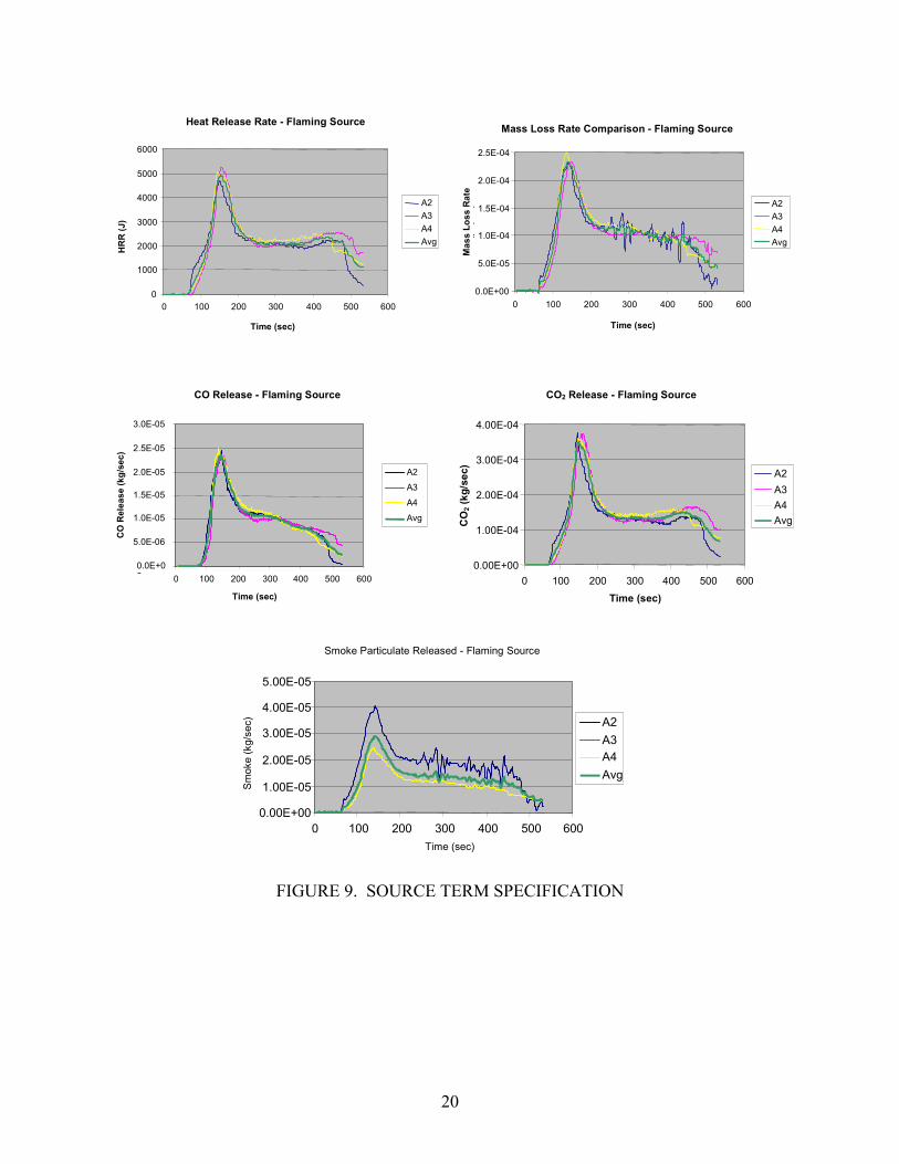
FIGURE 8. BASELINE COMPUTATIONAL MESH A flaming fire event occurring over 300 seconds was simulated using the computational model. The specification of the flaming fire source resulted from extensive cone calorimeter experiments at the FAA Technical Center. The fire is specified as a source term with parameters, shown in figure 9 (note that the fire ignition is at 60 seconds). The average of the three flaming fire data sets was used as the source term for the baseline calculations. Extensive data within the computational domain results from the simulation. For each time step, at each of the 24,000 cells, the user has access to values for the velocity (u, v, w), density, temperature, turbulence parameters, soot, CO, and CO2. An example of the temperature results within a plane of the computational domain is shown in figure 10. The K-plane shown is at the centerline of the fire, and the progression of the ceiling jet and the depth of the smoke layer are visible in the image.

19

Heat Release Rate - Flaming Source

0 1000 2000 3000 4000 5000 6000

0 100 200 300 400 500 600

Time (sec)

HR

R (J

)

A2A3A4Avg

Mass Loss Rate Comparison - Flaming Source

0.0E+00

5.0E-05

1.0E-04

1.5E-04

2.0E-04

2.5E-04

0 100 200 300 400 500 600

Time (sec)

Mas

s Lo

ss R

ate

(k/

) A2A3A4Avg

CO Release - Flaming Source

0.0E+00

5.0E-06 1.0E-05 1.5E-05 2.0E-05 2.5E-05 3.0E-05

0 100 200 300 400 500 600

Time (sec)

CO

Rel

ease

(kg/

sec)

A2A3

A4Avg

CO2 Release - Flaming Source

0.00E+00

1.00E-04

2.00E-04

3.00E-04

4.00E-04

0 100 200 300 400 500 600Time (sec)

CO

2 (kg

/sec

) A2A3A4Avg

Smoke Particulate Released - Flaming Source

0.00E+00 1.00E-05 2.00E-05 3.00E-05 4.00E-05 5.00E-05

0 100 200 300 400 500 600Time (sec)

Smok

e (k

g/se

c)

A2A3A4Avg

FIGURE 9. SOURCE TERM SPECIFICATION

20

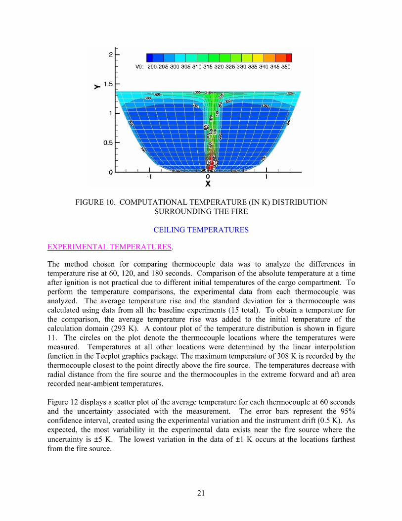
FIGURE 10. COMPUTATIONAL TEMPERATURE (IN K) DISTRIBUTION SURROUNDING THE FIRE

CEILING TEMPERATURES

EXPERIMENTAL TEMPERATURES.

The method chosen for comparing thermocouple data was to analyze the differences in temperature rise at 60, 120, and 180 seconds. Comparison of the absolute temperature at a time after ignition is not practical due to different initial temperatures of the cargo compartment. To perform the temperature comparisons, the experimental data from each thermocouple was analyzed. The average temperature rise and the standard deviation for a thermocouple was calculated using data from all the baseline experiments (15 total). To obtain a temperature for the comparison, the average temperature rise was added to the initial temperature of the calculation domain (293 K). A contour plot of the temperature distribution is shown in figure 11. The circles on the plot denote the thermocouple locations where the temperatures were measured. Temperatures at all other locations were determined by the linear interpolation function in the Tecplot graphics package. The maximum temperature of 308 K is recorded by the thermocouple closest to the point directly above the fire source. The temperatures decrease with radial distance from the fire source and the thermocouples in the extreme forward and aft area recorded near-ambient temperatures. Figure 12 displays a scatter plot of the average temperature for each thermocouple at 60 seconds and the uncertainty associated with the measurement. The error bars represent the 95% confidence interval, created using the experimental variation and the instrument drift (0.5 K). As expected, the most variability in the experimental data exists near the fire source where the uncertainty is ±5 K. The lowest variation in the data of ±1 K occurs at the locations farthest from the fire source.

21

FIGURE 11. EXPERIMENTAL TEMPERATURE DISTRIBUTION AT 60 SECONDS (Average rise + 293 K)

280

285

290

295

300

305

310

315

320

325

330

0 5 10 15 20 25 30 35 40

Thermocouple Number

Tem

pera

ture

(K)

60 s - Exp

FIGURE 12. CEILING TEMPERATURE AND VARIABILITY AT 60 SECONDS Figures 13 and 14 show the experimental thermocouple temperatures at 120 and 180 seconds after ignition. The trends in the temperature distribution are similar to the earlier time, but there is slightly less variability in the experimental data. The lowest temperatures are recorded at 60 seconds after ignition. The temperatures are higher at 120 seconds after ignition, but a reduced increase is observed from 120 to 180 seconds after ignition.

22

280

285

290

295

300

305

310

315

320

325

330

0 5 10 15 20 25 30 35 40

Thermocouple Number

Tem

pera

ture

(K)

120 s - Exp

FIGURE 13. CEILING TEMPERATURE AND VARIABILITY AT 120 SECONDS

280

285

290

295

300

305

310

315

320

325

330

0 5 10 15 20 25 30 35 40

Thermocouple Number

Tem

pera

ture

(K)

180 s - Exp

FIGURE 14. CEILING TEMPERATURE AND VARIABILITY AT 180 SECONDS COMPUTATIONAL TEMPERATURES.

The computational model results were analyzed to determine the temperature distribution near the ceiling of the cargo compartment. A contour plot of the gas temperature at 60 seconds, one cell below the ceiling (0.7″), is shown in figure 15. This contour contains all the information

23

available for the computational domain (i.e., temperature at every cell); therefore, it is much more detailed than the experimental results, which only contain temperatures interpolated from 40 points.

Temp (K):

FIGURE 15. COMPUTATIONAL TEMPERATURE DISTRIBUTION NEAR THE CEILING AT 60 SECONDS

Contour plots of the ceiling temperature distribution at 120 and 180 seconds after ignition are shown in figures 16 and 17. The region experiencing temperatures above 320 K increased compared with the corresponding result at 60 seconds after ignition. The wall temperature in the simulation was 293 K and is observed as the cooler region at the perimeter of the contour plots.

Temp (K):


24

Temp (K):


It is not desirable to compare the above contour plots directly to experimental contour plots since it contains many more data points and far less interpolation. A better visual comparison can be made by creating a contour plot of data sampled only at the instrumentation locations. The temperature values at 40 points, corresponding to the thermocouple locations, were sampled to create the contour plot shown in figure 18 (at 60 seconds after ignition). In comparing the contour plot of the computational temperature distribution to the experimental temperature distribution, it is evident that the computational temperatures are consistently higher. It is also evident that the highest temperatures in the domain are not captured by the instrumentation placement (note that the maximum temperature in figure 18 is 312 K, while the maximum temperature in figure 15 is 320 K). Therefore, it is critical that comparisons are made only at the instrumentation points.

FIGURE 18. CONTOUR PLOT OF COMPUTATIONAL GAS TEMPERATURES SAMPLED

AT THERMOCOUPLE LOCATIONS

25

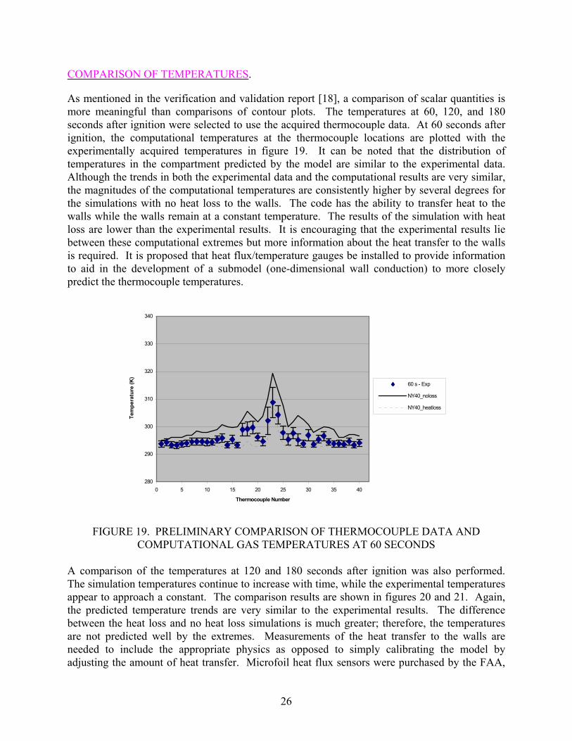
COMPARISON OF TEMPERATURES.

As mentioned in the verification and validation report [18], a comparison of scalar quantities is more meaningful than comparisons of contour plots. The temperatures at 60, 120, and 180 seconds after ignition were selected to use the acquired thermocouple data. At 60 seconds after ignition, the computational temperatures at the thermocouple locations are plotted with the experimentally acquired temperatures in figure 19. It can be noted that the distribution of temperatures in the compartment predicted by the model are similar to the experimental data. Although the trends in both the experimental data and the computational results are very similar, the magnitudes of the computational temperatures are consistently higher by several degrees for the simulations with no heat loss to the walls. The code has the ability to transfer heat to the walls while the walls remain at a constant temperature. The results of the simulation with heat loss are lower than the experimental results. It is encouraging that the experimental results lie between these computational extremes but more information about the heat transfer to the walls is required. It is proposed that heat flux/temperature gauges be installed to provide information to aid in the development of a submodel (one-dimensional wall conduction) to more closely predict the thermocouple temperatures.

280

290

300

310

320

330

340

0 5 10 15 20 25 30 35 40

Thermocouple Number

Tem

pera

ture

(K)

60 s - Exp

NY40_noloss

NY40_heatloss

FIGURE 19. PRELIMINARY COMPARISON OF THERMOCOUPLE DATA AND COMPUTATIONAL GAS TEMPERATURES AT 60 SECONDS

A comparison of the temperatures at 120 and 180 seconds after ignition was also performed. The simulation temperatures continue to increase with time, while the experimental temperatures appear to approach a constant. The comparison results are shown in figures 20 and 21. Again, the predicted temperature trends are very similar to the experimental results. The difference between the heat loss and no heat loss simulations is much greater; therefore, the temperatures are not predicted well by the extremes. Measurements of the heat transfer to the walls are needed to include the appropriate physics as opposed to simply calibrating the model by adjusting the amount of heat transfer. Microfoil heat flux sensors were purchased by the FAA,

26

and four sensors will be placed within the cargo compartment during future experiments. Initial locations for the measurements were selected to be directly above the fire and 5 feet from the point where the fire plume impacts the ceiling.

280

290

300

310

320

330

340

0 10 20 30 40 50

Thermocouple Number

Tem

pera

ture

(K)

120 s - ExpNY40_nolossNY40_heatloss


280

290

300

310

320

330

340

0 5 10 15 20 25 30 35 40

Thermcouple Number

Tem

pera

ture

(K)

180 s - ExpNY40_nolossNY40_heatloss


27

Additional potential causes for the discrepancy between the model and the experiments were identified. One likely cause for this discrepancy is that the presented computational temperatures are gas temperatures, not thermocouple temperatures. The correction of the gas temperatures to thermocouple temperatures requires knowledge of the gas velocities and density. The model output was used to make this correction, and it was determined that the thermocouples are sufficiently small, thus, the correction is negligible. An alternate reason for the difference between the computational and experimental results is the manner in which temperatures are determined in the model. Currently, the temperature calculation is based on user-entered constant species heat capacities (i.e., h = Int(Cp(T)dT) ===> T = h/Cp_av). The specific heats and molecular weights of the pure species entered will be evaluated to determine that they are correct and are not adversely impacting the temperature calculation. Currently, the user-defined specific heats are as follows: soot = 600.7, CO2 = 851.7, CO = 1043, and air = 1007 J/kg-K. The mixture-specific heats and molecular weights were evaluated at the source cell. The conclusion is that the mixture fractions are so small for the nonair species that they have very little impact on the mixture values. After 100 seconds, there was only a 0.06% change in the mixture-specific heat between runs that adjusted the specific heat of soot by a factor of 6. Another potential reason for the difference in temperature is the omission of radiation from the fire source in the calculations. Literature reveals that radiation from fires can approach 30% of the heat release. Experiments that investigate the radiation loss from the fire are proposed. A hot plate test, where radiation is negligible, could determine if temperatures are adequately predicted. An assessment of the radiation loss from the fire can be obtained by performing heat flux measurements in the experiments. Lastly, photographs of the thermocouples show that they appear to be heavily coated with soot, which could impact the temperature measurements. It is recommended that the FAA observe two thermocouples that are close enough together that they basically read the same value, and for a subsequent test, clean one and not the other to see if they read differently, at least initially. This soot could insulate the thermocouple from convection or alter it due to the increased surface area and increase the area and emissivity for radiation. These effects may offset one another, but if it is determined that the soot does appear to make a difference, then they should be cleaned between tests. The FAA has recently investigated the impact of the soot coating on thermocouple measurements as recommended above. A photograph of a thermocouple (coated with soot) in the full-scale test fixture is shown in figure 22. Several tests were performed in which the thermocouple at a location was either coated with soot or clean. Experiments were performed with the fire located directly under the thermocouple and 5 feet away. Figure 23 shows the results from when the fire was directly under the thermocouple. There is good repeatability in the experiments and the clean and sooty thermocouples record the same temperatures. The same is true when the fire is located 5 feet away, as shown in figure 24. However, while performing the thermocouple investigation, it was noticed that some thermocouple beads were covered by an insulating sheath. The thermocouples used to assess the effect of soot on the bead, as described above, were not affected by this problem. Further experiments revealed that the covered beads

28

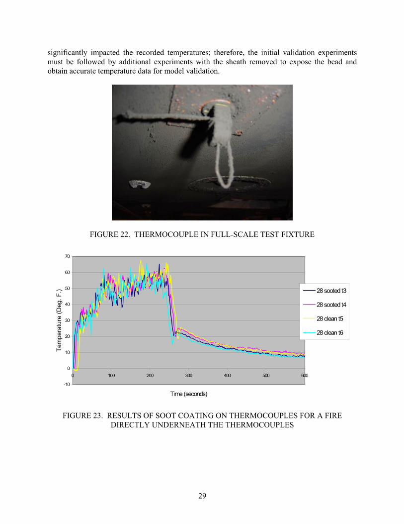
significantly impacted the recorded temperatures; therefore, the initial validation experiments must be followed by additional experiments with the sheath removed to expose the bead and obtain accurate temperature data for model validation.

FIGURE 22. THERMOCOUPLE IN FULL-SCALE TEST FIXTURE

-10

0

10

20

30

40

50

60

70

0 100 200 300 400 500 600

Time (seconds)

Tem

pera

ture

(Deg

. F.) 28 sooted t3

28 sooted t4

28 clean t5

28 clean t6

FIGURE 23. RESULTS OF SOOT COATING ON THERMOCOUPLES FOR A FIRE DIRECTLY UNDERNEATH THE THERMOCOUPLES

29

-5

0

5

10

15

20

25

30

0 100 200 300 400 500 600

Time (seconds)

Deg

. F. 28 sooted t1

28 sooted t2

28 clean t7

28 clean t8

FIGURE 24. RESULTS OF SOOT COATING ON THERMOCOUPLES FOR A

FIRE LOCATED 5 FEET AWAY

LIGHT TRANSMISSION

EXPERIMENTAL LIGHT TRANSMISSION.

The light transmission was measured experimentally at six locations, as described in table 2. The selected validation metrics for light transmission are: • 30 and 45 seconds (ceiling and vertical) • 60 seconds (vertical—high, mid, low) • 120 seconds (vertical—mid and low) • 180 seconds (vertical—mid and low) Experimental results are presented in this section. Uncertainty bars have been placed on the experimental measurements, which include the experimental variability and instrument drift. An assessment of the total uncertainty has not been performed since calibration data sets were not available for all baseline experiments. Instrument drifts were 0.1% for ceiling forward, ceiling mid, and vertical mid; 0.4% for vertical high and ceiling aft; and 0.2% for vertical low. Experimental measurements and measurement uncertainties are shown in table 3. Uncertainty in the operation of the diagnostic is quite high for measurements below 80% light transmission; thus, all comparisons were made above this level. Measurements below 80% are shown in gray.

TABLE 3. EXPERIMENTAL LIGHT TRANSMISSION DATA %LT 30s_EXP 30s Error 45s_EXP 45s Error 60s_EXP 60s Error 120s_EXP 120s Error 180s_EXP 180s ErrorC-fwd 97.3 3.5 89.6 5.2 80.3 4.9 65.1 3.8 60.8 3.9 C-mid 94.9 3.8 87.1 5.5 78.6 4.6 63.4 5.1 59.8 3.1 C-aft 95.9 3.7 87.9 6.0 79.1 6.0 63.9 4.3 60.7 4.3 V-High 99.9 0.8 99.9 1.0 97.7 3.1 73.8 6.3 64.4 5.3 V-Mid 100.0 0.2 100.0 0.2 99.9 0.3 95.5 3.9 87.6 10.1 V-low 99.9 0.5 99.9 0.5 99.9 0.5 99.8 0.6 97.5 2.1

30

COMPUTATIONAL LIGHT TRANSMISSION.

Light transmission is not directly calculated in the computational model; instead, the model results are postprocessed to determine the light transmission at the time of interest. Smokemeter readings were calculated by integrating soot concentration information for the cells located along the beam path. Output from individual computational cells was used to determine percent light transmission (the value measured in the experiments) for the predicted field values using Beer’s Law.

scellsootdx)x(k )x()x(C)x(kwhere

II

eL

σρ0

0

== ∫−

where sσ is the specific extinction coefficient (7400 kgm2

), is the soot concentration (sootCkgkg ),

and ρcell is the gas density ( 3mkg ).

The specific extinction coefficient value is based upon earlier research on the soot morphology and optical properties. The coefficient was determined using the soot morphology from the flaming resin and the Rayleigh-Debye-Gans theory for polydisperse fractal aggregates (RDG-PFA). The values for Csoot and ρcell are output for each cell at each time step in the simulation. A computer code was written to perform the calculation for the decrease in light transmission from the sum of the individual cells along the beam path of the smokemeter. In accordance with the procedure used by the FAA, the intensity ratio was then raised to the 1/L power (with L in feet).

L

dxk

L

L

eIIft/%LT

∫ ⋅−

⋅=

⋅=

0

100100

1

0

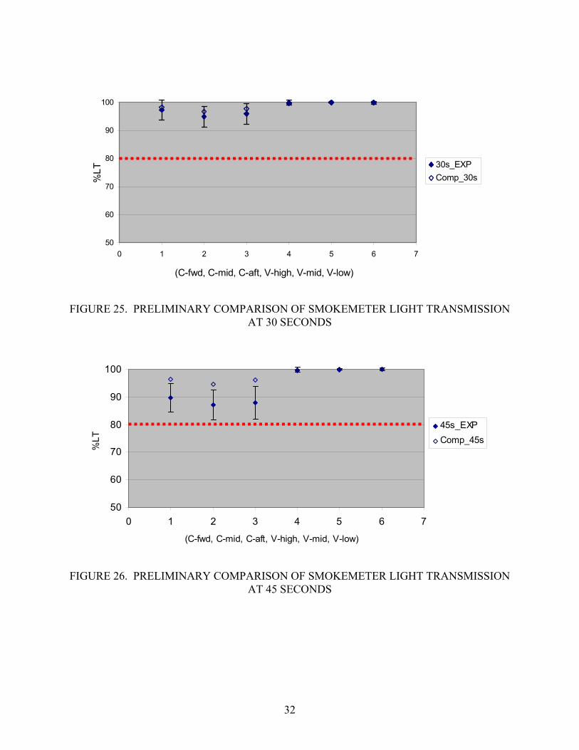
COMPARISON OF LIGHT TRANSMISSION.

The percent light transmission validation metrics were used in the comparison of experimental data to computational results. Computational data for the ceiling smokemeters are available at y = 1.32 m, which is approximately 0.01 m (0.4″) higher than the experimental measurements. The vertical smokemeter calculations are presented at x = 4.93 m, which is 0.03 m (1.2″) further aft in the compartment. If not stated, other presented predictions are in the exact same location as the experimental measurements. Since comparisons were not made where the experimental data were below the 80% dotted line, those smokemeter readings are omitted. The comparisons are shown in figures 25-29.

31

50

60

70

80

90

100

0 1 2 3 4 5 6 7

(C-fwd, C-mid, C-aft, V-high, V-mid, V-low)

%LT

30s_EXPComp_30s

FIGURE 25. PRELIMINARY COMPARISON OF SMOKEMETER LIGHT TRANSMISSION AT 30 SECONDS

50

60

70

80

90

100

0 1 2 3 4 5 6 7

(C-fwd, C-mid, C-aft, V-high, V-mid, V-low)

%LT

45s_EXPComp_45s

FIGURE 26. PRELIMINARY COMPARISON OF SMOKEMETER LIGHT TRANSMISSION

AT 45 SECONDS

32

50

60

70

80

90

100

(V-high, V-mid, V-low)

%LT

60s_EXPComp_NY40

FIGURE 27. PRELIMINARY COMPARISON OF SMOKEMETER LIGHT TRANSMISSION

AT 60 SECONDS

50

60

70

80

90

100

(V-mid, V-low)

% L

T 120s_EXP120s_Comp


50

60

70

80

90

100

(V-mid, V-low)

% L

T 180s_EXP180s_Comp


33

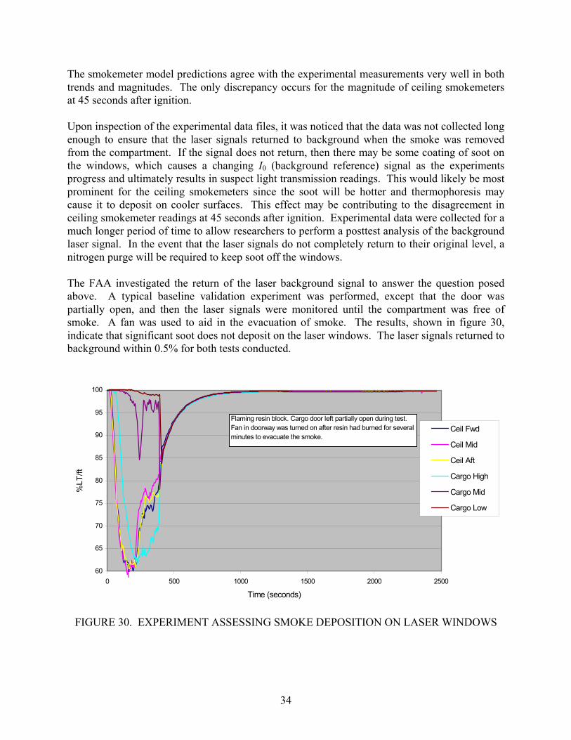
The smokemeter model predictions agree with the experimental measurements very well in both trends and magnitudes. The only discrepancy occurs for the magnitude of ceiling smokemeters at 45 seconds after ignition. Upon inspection of the experimental data files, it was noticed that the data was not collected long enough to ensure that the laser signals returned to background when the smoke was removed from the compartment. If the signal does not return, then there may be some coating of soot on the windows, which causes a changing I0 (background reference) signal as the experiments progress and ultimately results in suspect light transmission readings. This would likely be most prominent for the ceiling smokemeters since the soot will be hotter and thermophoresis may cause it to deposit on cooler surfaces. This effect may be contributing to the disagreement in ceiling smokemeter readings at 45 seconds after ignition. Experimental data were collected for a much longer period of time to allow researchers to perform a posttest analysis of the background laser signal. In the event that the laser signals do not completely return to their original level, a nitrogen purge will be required to keep soot off the windows. The FAA investigated the return of the laser background signal to answer the question posed above. A typical baseline validation experiment was performed, except that the door was partially open, and then the laser signals were monitored until the compartment was free of smoke. A fan was used to aid in the evacuation of smoke. The results, shown in figure 30, indicate that significant soot does not deposit on the laser windows. The laser signals returned to background within 0.5% for both tests conducted.

60

65

70

75

80

85

90

95

100

0 500 1000 1500 2000 2500

Time (seconds)

%LT

/ft

Ceil Fwd

Ceil Mid

Ceil Aft

Cargo High

Cargo Mid

Cargo Low

Flaming resin block. Cargo door left partially open during test. Fan in doorway was turned on after resin had burned for several minutes to evacuate the smoke.

FIGURE 30. EXPERIMENT ASSESSING SMOKE DEPOSITION ON LASER WINDOWS

34

Beam steering was identified as a potential source of uncertainty. The FAA conducted an experiment with a heat gun that produced the same temperature rise as the fire in the compartment. The experiment showed no impact on the smokemeter readings, thus beam steering is negligible. As mentioned previously, the error bars on the experimental data include only experimental variability and instrument drift. Calibration data sets for each experiment would allow an assessment of the total uncertainty. Currently, the smokemeters are only calibrated if a laser or detector in the system is replaced. It was requested that the smokemeter calibrations be performed more frequently. A calibration file, including pre- and posttest calibrations, for a single experiment was provided and is shown in figure 31. The smokemeters produce consistent readings in the calibrations before and after the fire experiment. The readings are typically within 2% of the target value, which is produced by a filter that is held in front of the laser detector.

70

75

80

85

90

95

100

50 100 150 200 250

Time (seconds)

%LT

/ft

High pretestHigh posttest97.795.593.391.179.3

FIGURE 31. SMOKEMETER CALIBRATION FILE

GAS CONCENTRATIONS

EXPERIMENTAL GAS CONCENTRATIONS.

The average rise in experimental gas concentrations from five replicate experiments was computed at 60, 120, and 180 seconds after ignition. The results are shown in tables 4 through 6. The uncertainty in the experimental results include experimental variability, instrument accuracy, and instrument drift. The accuracy of the instrument was obtained from the manufacturer as ±1% of the range. The range for CO was 500 ppm, and the range for CO2 was 2500 ppm.

35

TABLE 4. EXPERIMENTAL GAS CONCENTRATIONS AT 60 SECONDS (All measurements in ppm)

CO Exp EXP-SD (±1% range) Drift Uncert bar Aft Pan 78.4 8.8 5.0 0.3 20.3 Mid Pan 52.5 16.5 5.0 0.3 34.6 TC36 29.4 7.3 5.0 0.3 17.8

CO2 Exp EXP-SD (±1% range) Drift Uncert bar Aft Pan 793.2 165.4 25.0 3.5 334.7 Mid Pan 556.0 72.8 25.0 3.5 154.2 TC36 451.7 50.5 25.0 3.5 113.0

TABLE 5. EXPERIMENTAL GAS CONCENTRATIONS AT 120 SECONDS

(All measurements in ppm)



TABLE 6. EXPERIMENTAL GAS CONCENTRATIONS AT 180 SECONDS

(All measurements in ppm)



36

COMPUTATIONAL GAS CONCENTRATIONS.

The gas concentrations of interest in the computations are CO and CO2. The computational model predicts the concentration of these gases in terms of a mass fraction (kg/kg), while the experimental results are in terms of volume fraction (ppm). The computational concentrations are converted to the experimental concentration units using the following equations.

gas

cellgasgas kg

kginCmminC

ρρ

×= )()( 3

3

where ρcell is obtained from the computational output and the densities of CO and CO2 are 1.145 kg/m3 and 1.833 kg/m3, respectively. The computational gas concentrations were extracted from the simulation domain at locations corresponding to the gas analyzer locations. Mid and aft concentrations were obtained in the recessed area, which is currently not modeled; therefore, those concentrations were obtained just below the ceiling level. The corner gas sampling location was very close to the experimental sampling location. COMPARISON OF GAS CONCENTRATIONS.

The gas concentrations, as measured in three locations (mid pan, aft pan, and TC36), were compared to the computational predictions at 60, 120, and 180 seconds after ignition. The rises in gas concentrations were compared since the starting concentrations varied for each experiment. The comparisons of the gas concentrations are shown in figures 32 through 34.

CO at 60 sec

0

25

50

75

100

125

150

175

200

0 1 2 3 4

Position (Aft, Mid, TC36)

Con

cent

ratio

n (p

pm)

Exp

Comp_NY40

CO2 at 60 sec

0

200

400

600

800

1000

1200

0 1 2 3 4


Con

cent

ratio

n (p

pm)

Exp

Comp_NY40

FIGURE 32. PRELIMINARY COMPARISON OF GAS CONCENTRATIONS AT 60 SECONDS

37

CO at 120 sec

0

25

50

75

100

125

150

175

200

0 1 2 3 4


Con

cent

ratio

n (p

pm)

Exp

Comp NY40

CO2 at 120 sec

0

200

400

600

800

1000

1200

1400

1600

0 1 2 3 4


Con

cent

ratio

n (p

pm)

Exp

Comp NY40


CO at 180 sec

0

25

50

75

100

125

150

175

200

0 1 2 3 4


Con

cent

ratio

n (p

pm)

Exp

Comp NY40

CO2 at 180 sec

0

200

400

600

800

1000

1200

1400

1600

1800

0 1 2 3 4


Con

cent

ratio

n (p

pm)

Exp

Comp NY40


The agreement in the magnitude of the CO gas concentration readings are fair at 60 seconds after ignition, although the trends are different. At later times, the agreement of the trends is better, but the magnitudes are less favorable (especially for CO2). Overall, the gas concentration predictions were not satisfactory. Several potential reasons for the disagreement are noted. First, the recessed areas are not currently being modeled. Code predictions are presented one cell below the ceiling. Previous studies have shown the recessed areas impact the flow field. Therefore, the recessed areas are being added to the model. Second, there is some lag in the gas analyzer readings due to transport times through the line and instrument response. The transport time of 8 seconds was subtracted from the experimental data to adjust for the lag in response due to line transport. An adjustment was not made to account for the delay due to instrument response. The gas concentration signal can be deconvoluted to account for instrument response using the data on the instrument response to a step function. The recorded and adjusted signals are shown in figure 35. Due to the nature of the signal, the

38

adjusted signal is smoother than the recorded signal, but there is no significant change when the signal is deconvoluted. Therefore, experimental gas analyzer signals will not need to be deconvoluted for future experiments.

0

10

20

30

40

50

60

70

80

90

100

0 50 100 150 200 250 300

Adjusted Signal

Recorded Signal

FIGURE 35. DECONVOLUTION OF ANALYZER SIGNAL

Third, a potential source of uncertainty is that the flaming resin block may burn differently in the cargo compartment than in the cone calorimeter. Since the cone calorimeter data are used as input to the model, any difference in the local ventilation and the thermal environment in the compartment would introduce error into the calculation boundary condition and results. The FAA compared the CO2/CO ratios between the cone data and the B707 and determined that they were similar (around 11 to 14), indicating that the cone is not overventilated and the species generation rates apply to the B707 tests as well. Fourth, it was observed that some items in the cargo compartment may be impacting the flow and transport of smoke. Experimental data would benefit from a removal or relocation of some items. The lamp that is placed on the floor of the cargo compartment should be removed. It is likely that the line for the gas sample is considerably affecting the transport of smoke and gas species since it is quite large and is attached to the ceiling. An indication of this is evident in the trends of the gas readings. The experimental gas concentrations in the aft pan are consistently higher than the mid pan. This result is counter-intuitive because the mid pan is closer to the fire source. It is possible that the ceiling jet flow interacts with the line causing the smoke to be transported differently. Additional experimental data sets will be obtained with the line repositioned to determine if there was an impact on the gas concentrations and the agreement between experimental and computational data.

39

The cargo compartment has been modified to address the factors stated above. Most significantly, the gas analyzer line now collects samples from a fitting in the recessed area. The entire line is routed through the area above the cargo compartment, thus keeping the ceiling free of obstructions.

CONCLUSIONS

This document provided an overview of the smoke transport model, including the computational transport solver and the graphical user interface. In addition, preliminary baseline validation experimental data and model predictions were documented. Validation metrics were selected and initial comparisons between the experimental and computational results were performed using these metrics. The agreement between the experimental and computational results provides some confidence in the code results. Results of the initial comparisons indicate that additional experiments must be conducted to produce true validation and determine that the model captures the dominant physical mechanisms. A number of potential improvements in experimental data were identified and modifications to the cargo compartment were performed; therefore, an additional set of experiments will be performed. Modifications to the computational model include the addition of recessed areas and potentially a wall-conduction submodel. Comparisons of model calculations with the new experimental results will be documented when additional baseline experiments are completed. The resulting validated smoke transport model will be used to enhance the smoke detection system certification process by determining worst-case locations for fires, optimum placement of fire detector sensors within the cargo compartment, and sensor alarm levels needed to achieve detection within the required certification time.

REFERENCES

1. Code of Federal Regulations 14 CFR Part 25.858.

2. Bird, R.B., Steward, W.E., and Lightfoot, E.N., Transport Phenomena, John Wiley and Sons, New York, 1960.

3. Gatski, T.B., Grosch, C.E., and Rose, M.E., J. Comp. Phys., 82:298, 1989.

4. Favre, A., “Problems of Hydrodynamics and Continuum Mechanics,” Society of Indiustrial and Applied Mathematics, Philidelphia, PA, 1969.

5. Bilger, R.W., Prog. Energy Combust. Sci., 1:88, 1976.

6. Launder, B.E. and Spalding, D.B., “The Numerical Computation of Turbulent Flows,” Computer Methods in Applied Mechanics and Engineering, 3:269, 1974.

7. DesJardin, P.E., Nelsen, J.M., Gritzo, L.A., Lopez, A.R., Suo-Anttila, J.M., Keyser, D.R., Ghee, T.A., Disimile, P.J., and Tucker, J.R., Proceedings of the Halon Options Technical Working Conference, 99-110, 2001.

40

8. Kuwahara, F., Kameyama, Y., Yamashita, S., and Nakayama, A., J. of Porous Meda, 1:47-55, 1998.

9. Ergun, S., Chem. Eng. Prog., 48:89-94, 1952.

10. Patankar, S.V., Numerical Heat Transfer and Fuid Flow, Taylor and Francis, New York, 1980.

11. Rhie, C.M. and Chow, W.L., AIAA Journal, 21:1525-1532, 1983.

12. Parameswaran, S., Srinivasan, A.B., and Sun, R.L., N. H. T. Part A, 21:443, 1992.

13. Versteg, H.K. and Malalasekera, W., An Introduction to Computational Fluid Dynamics, Longman, London, 1999.

14. Stone, H., SIAM J. Numer. Anal., 5(3):530, 1968.

15. Ferziger, J.H. and Peric, M., Computational Methods for Fluid Dynamics, Springer, New York, 1999.

16. Launder, B.E. and Spalding, D.B., Mathematical Models of Turbulence, Academic Press, London, 1972.

17. Suo-Anttila, J.M. and Gill, W., “Experimental Data for Baseline Validation,” internal memorandum to David Blake, September 2002.

18. Suo-Anttila, J.M., Gill, W., Domino, S.P., DesJardin, P.E., and Gritzo, L.A., “A Preliminary Verification and Validation for the FAA Smoke Tranpsort Code,” internal report to David Blake, September 2001.

41/42

dot/faa/ar-03/49 computational fluid dynamics code for

Documents