download (225kb) - munich personal repec archive

Munich Personal RePEc Archive

Bank Efficiency and Share Prices in

China: Empirical Evidence from a

Three-Stage Banking Model

Abdul Majid, Muhamed Zulkhibri and Sufian, Fadzlan

Central Bank of Malaysia, University Putra Malaysia

1 March 2008

Online at https://mpra.ub.uni-muenchen.de/12120/

MPRA Paper No. 12120, posted 12 Dec 2008 19:47 UTC

Bank Efficiency and Share Prices in China: Empirical Evidence from a


MUHAMED-ZULKHIBRI ABDUL MAJID a

Central Bank of Malaysia, Malaysia

University of Nottingham, U.K

FADZLAN SUFIAN b, c

CIMB Bank Berhad, Malaysia

Universiti Putra Malaysia, Malaysia

Corresponding author: a Senior Economist in Monetary and Financial Policy Department, Central Bank of Malaysia.

Mailing address: Monetary and Financial Policy Department, Bank Negara Malaysia, Jalan Dato’ Onn, 50480 Kuala

Lumpur, Malaysia. e-mail: [email protected]; [email protected]

Tel: 603-2698-8044; Fax: 603-2693-5023 b Planning and Research Department, CIMB Bank Berhad c Department of Economics, Faculty of Economics and Management, Universiti Putra Malaysia.

Mailing address: 21st Floor, 6 Jalan Tun Perak, 50050 Kuala Lumpur, Malaysia.

e-mail: [email protected]; [email protected]

Tel: 603-2693-1722 (ext: 6455); Fax: 603-2691-4415 # All findings, interpretations, and conclusions are solely of the authors’ opinion and do not necessarily represents

the views of the institutions.

1

Bank Efficiency and Share Prices in China: Empirical Evidence from a


ABSTRACT

This paper examines for the first time the relationship between China banks’ efficiency and its share price

performance. Our analysis consists of three parts. First, we calculate the annual share price returns of the

banks for each year between 1997 and 2006. Then we employ Data Envelopment Analysis (DEA)

Window Analysis method, first proposed by Charnes et al. (1985) to estimate the efficiency of the banks.

Finally, we estimate the annual share price returns over the change in efficiency, while controlling for

other bank specific traits. The empirical findings suggest that large China banks have exhibited higher

technical and pure technical efficiency levels compared to their small and medium sized bank

counterparts, while the medium sized banks have exhibited higher scale efficiency. The relationship

between China banks’ efficiency and share price performance suggest that bank efficiency estimates

derived from the DEA Window Analysis method contributes significant information towards share price

returns beyond that provided by financial information.

JEL Classification: G21

Keywords: Bank Efficiency, Share Prices, DEA Window Analysis, China

2

1. INTRODUCTION

Studies on the stock market have found that stock prices do incorporate relevant publicly known

information (Ball and Kothari, 1994). An efficient stock market should consider operating efficiency

measures in the price formation process, as they represent all publicly available information. All else

being equal, relatively more efficient banks should be able to raise capital at a lower cost. In a semi-

strong, efficient market where most of the information is incorporated into prices, share price

performance is the best measure whether firms are creating value for shareholders or not (Brealey and

Myers, 1991). Thus, it may be expected that efficient firms perform better than inefficient firms and this

will be reflected in market prices (directly through lower costs or higher output or indirectly through

higher customer satisfaction and higher prices which in return may improve share price performance).

Although quite exhaustive surveys exist in the literature to examine the relationship between

traditional accounting performance measures and share price changes1, only a handful of studies have

examined the relationship between bank efficiency and share price performance (Beccalli et al. 2006).

These include Adenso-Diaz and Gascon (1997) in Spain, Chu and Lim (1998) in Singapore, Eisenbeis et

al. (1999) in the U.S., Beccalli et al. (2006) in the principal EU banking sectors (i.e. France, Germany,

Italy, Spain, and U.K), Sufian and Majid (2006) in Malaysia, Kirkwood Nahm (2006) in Australia, and

Pasiouras et al. (2007) on Greece.

The present study contributes to the existing literature in at least three important ways. First,

despite the importance of the China banking sector to the domestic, regional, and international economies,

there are only a few microeconomic studies performed in this area of research. This study thus attempts to

fill a demanding gap by providing the most recent evidence on the performance of the China banking

sector. Second, unlike the previous studies on China banks’ efficiency, the present study attempts to

examine the efficiency of the China banking sector by using the Data Envelopment Analysis (DEA)

Window Analysis method, first proposed by Charnes et al. (1985). Given the small sample size of the

China listed banks, we believe that it is more appropriate to investigate the efficiency of the China

banking sector by using the DEA Window Analysis method for at least two important reasons. Firstly, the

method provides a greater degree of freedom to the sample (Reisman, 2003). Secondly, the greater degree

of freedom could provide better explanatory power to the second stage regression analysis (Sufian, 2007).

Nevertheless, this study will also be the first to investigate the efficiency of the China banking sector by

using this relatively new DEA Window Analysis method. And finally, the study attempt to examine the

1 See Kothari (2001) for a very comprehensive review of the literature.

3

relationship between China banks’ efficiency and its share price performance in the marketplace. To the

best of our knowledge, this type of analysis is completely missing in the literature in regard to the China

banking sector.

This paper is set out as follows. The next section reviews related studies in the main literature

with respect to the study on bank efficiency. Section 3 outlines the approach to the measurement and

estimation of efficiency change and provides details on the construction of our data set. Section 4

discusses the results and finally, section 5 provides some concluding remarks.

2. SURVEY OF THE LITERATURE ON BANK EFFICIENCY

Studies on bank efficiency are fast growing, but the vast majority of studies cover the U.S. and

other developed countries (Berger et al. 1993; Berger and Humphrey, 1997). Although there have been a

number of studies examining the efficiency of the Chinese banking industry, these studies have been

published in Chinese scholarly journals2. To date, only a few studies are available to non-Chinese readers.

Among them are studies by Chen et al. (2005), Fu and Heffernan (2007), Ariff and Can (2007) and Yao et

al (2007).

Chen et al (2005) examined the cost, technical and allocative efficiency of 43 Chinese banks over

the period 1993 to 2000. The results show that the large state-owned banks and smaller banks are more

efficient than the medium sized Chinese banks. In addition, technical efficiency consistently dominates

the allocative efficiency of Chinese banks. The financial deregulation of 1995 was found to improve cost

efficiency levels including both technical and allocative efficiency.

Fu and Heffernan (2007) employed the Stochastic Frontier Approach (SFA) to investigate China

banking sector‘s cost X-efficiency over the period 1985 to 2002. A two-stage regression model is

estimated to identify the significant variables influencing X-efficiency. Overall, the results show that

banks are operating 40–60% below the X-efficiency frontier. On average, the joint-stock commercial

banks are found to be more X-efficient than the state-owned commercial banks, but individual scores

present a far more complex picture. It appears that X-efficiency was higher during the first phase of bank

reform. Recent policies aimed at increased privatization, greater foreign bank participation, and

liberalized interest rates should help to improve the cost X-efficiency of China banks.

2 For example Xue and Yang (1998), Zhao (2000), Wei and Wang (2000), Qing and Ou (2001), and Xu et al. (2001) have used the non-

parametric techniques, while Qian (2003), Liu and Song (2004), and Zhang et al. (2005) have used the parametric methods.

4

Ariff and Can (2007) used the non-parametric Data Envelopment Analysis (DEA) technique to

investigate the cost and profit efficiency of 28 Chinese commercial banks during the period 1995 to 2004.

In the second stage regression, they examine the influence of ownership type, size, risk profile,

profitability, and key environmental changes on bank efficiency by using the Tobit regression. They find

that profit efficiency levels are lower than cost efficiency, suggesting that the most important

inefficiencies are on the revenue side. They suggest that the joint-stock commercial banks (national and

city based) have exhibited higher cost and profit efficiency relative to their state-owned bank

counterparts. Likewise, they find that the medium sized banks are more efficient than their small and

large peers.

By employing the stochastic frontier production function, Yao et al. (2007) used a panel data of

22 banks over the period 1995-2001 to investigate the effects of ownership structure and hard budget

constraint on China banks’ efficiency. Their empirical results suggest that the non-state banks were 8-

18% more efficient than the state banks, and that banks facing a harder budget tend to perform better than

those heavily capitalized by the state or regional governments. The results shed important light on

banking sector reform in China facing up to the tough challenges after WTO accession.

2.1 Evidence on Bank Efficiency and Share Prices

Efficiency studies applied to banking sectors are abound in the literature. However, only a few studies

have examined the relationship between bank efficiency and its share price performance in the

marketplace (Beccalli et al. 2006). Using DEA with three inputs and two outputs, Chu and Lim (1998)

evaluated the relative cost and profit efficiency of a panel of six Singapore listed banks during the period

1992-1996. They found that during the period the six Singapore listed banks have exhibited higher overall

efficiency of 95.3% compared to profit efficiency of 82.6%. They also found that large Singapore banks

have reported higher efficiency of 99.0% compared to 92.0% for the small banks. They also suggested

that scale inefficiency dominates pure technical inefficiency during the period of study. They found that

percentage change in the price of bank shares reflect percentage change in profit rather than cost

efficiency.

By using the DEA and the parametric Stochastic Frontier Approach (SFA) method, Beccalli et al.

(2006) estimated efficiency measures of the banking cost to a sample of European banks (France,

Germany, Italy, Spain, and the UK) in 1999 and 2000. The definition of the parameters used in the model,

focused on the intermediation using deposits, loans, and securities as outputs, and labour and capital as

5

inputs. The authors made the regression of the annual scores of efficiency in relation to the respective

performances in the stock market. The results suggest that changes in the prices of banks’ stocks mirror

changes in cost efficiency, especially the ones derived from the DEA. This trend is less clear when the

SFA model is used.

Kirkwood and Nahm (2006) used Data Envelopment Analysis (DEA) to evaluate cost efficiency

of Australian banks in producing banking services and profit between 1995 and 2002. The empirical

findings indicate that the major banks have improved their efficiency in producing banking services and

profit, while the regional banks have experienced little change in the efficiency of producing banking

services, and a decline in the efficiency of producing profit. They further relate the changes in efficiency

to stock returns and found that change in bank efficiency is reflected in stock returns.

Sufian and Majid (2006) empirically investigated the cost and profit efficiencies of Malaysian

banks that are listed on the Kuala Lumpur Stock Exchange (KLSE) during 2002-2003 by applying the

non-parametric DEA model. They found that the cost efficiency of Malaysian banks was on average

significantly higher compared to profit efficiency. They also suggest that the large banking groups on

average were more cost efficient, whereas the smaller banking groups were found to be more profit

efficient. They suggest that the stock prices of Malaysian banks react more towards the improvements in

profit efficiency rather than the improvements in cost efficiency.

Pasiouras et al. (2007) examined the association between the efficiency of Greek banks and their

share price performance. Their sample of analysis comprised of the 10 Greece commercial banks, which

are listed on the Athens stock exchange. They found that the average technical efficiency under the

constant returns to scale is 93.1% and increases to 97.7% under variable returns to scale. The regression

results indicate a positive and statistically significant relationship between annual changes in technical

efficiency and share price returns. On the other hand, they found that changes in scale efficiency have no

impact on share price returns.

2.2 Bank Efficiency Studies Utilizing DEA Window Analysis

Although studies investigating bank efficiency using DEA are voluminous, there are only a few papers,

which have utilized the DEA Window Analysis method, first proposed by Charnes et al. (1985) to

banking. Among the notable microeconomic research performed were those by Reisman et al. (2003),

Webb (2003), Avkiran (2004), and Sufian (2007).

6

Reisman et al. (2003) investigated the impact of deregulation on the efficiency of eleven Tunisian

commercial banks during 1990 to 2001. Applying three inputs namely fixed assets, number of employees,

and deposits, loans and securities portfolios as outputs, they followed the intermediation approach to

DEA with an extended window analysis. They found that deregulation had a positive impact on Tunisian

commercial banks’ technical efficiency. They suggest that public banks outperformed private banks in

transforming deposits into loans. The decomposition of technical efficiency into its pure technical and

scale efficiency components indicate that private banks experienced predominantly pure technical

inefficiency during the period. The public banks on the other hand were pure technically inefficient

during the early period, which was mostly, scale inefficient towards the end of the period of study. They

also suggest that both public and private banks were inefficient in their investments.

Webb (2003) utilized DEA Window Analysis to investigate the relative efficiency levels of large

UK retail banks during the period of 1982-1995. Following the intermediation approach, three inputs are

considered namely deposits, interest expense, and operational expenses, while total income and total loans

are outputs. He found that during the period the mean inefficiency levels of UK retail banks were low

compared to past studies on UK banking industry. He suggested that the overall long run average

efficiency level is falling and that all the six large UK banks shows declining levels of efficiency over the

entire period. He concluded that scale inefficiency dominated pure technical inefficiency; less big banks

are more likely to report technical inefficiency, and during the period of study banks with asset levels of

over ₤105 billion suffered declining returns to scale (DRS).

Applying a three-year window to a sample of 10 Australian trading banks during the period 1986-

1995, Avkiran (2004) found that Australian trading banks have exhibited deteriorating efficiency levels

during the earlier part of the studies, before progressively trending upwards in the latter part. During the

period of study, he found that interest expenses to be the main source of inefficiency of Australian trading

banks. He suggest that most Australian banks have exhibited CRS during the early period, DRS and IRS

in the early 1990s and turn to exhibit CRS during the latter part of the studies.

More recently, Sufian (2007) investigated the long-term trend in the efficiency of the Singapore

banking groups over the period 1993-2003 by using the DEA Window Analysis approach. During the

period of study, he found that the Singapore banking groups have exhibited mean technical efficiency of

88.4%. The findings suggest that the Singapore banking groups’ technical efficiency was on a declining

trend during the earlier part of the study, before increasing during the later period. Overall, the results

suggest that scale inefficiency outweighs pure technical inefficiency in determining the Singapore

7

banking groups’ technical efficiency. The empirical findings also suggest that the small Singapore

banking groups outperformed their large and very large counterparts for all efficiency measures.

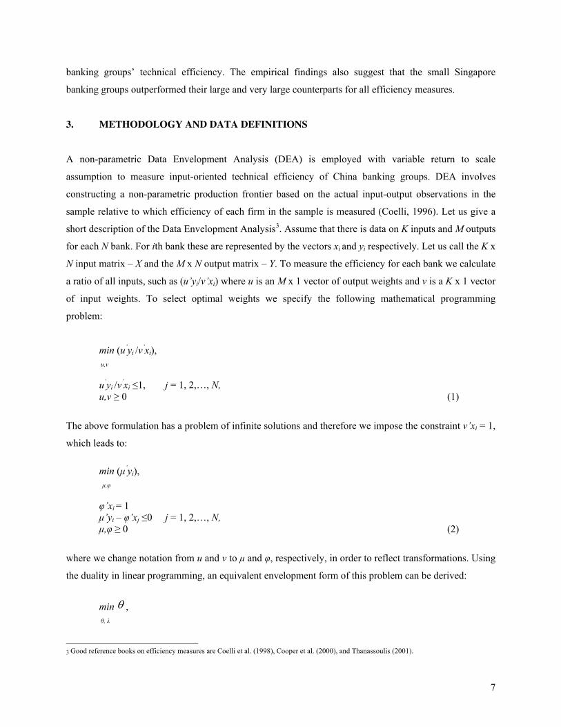
3. METHODOLOGY AND DATA DEFINITIONS

A non-parametric Data Envelopment Analysis (DEA) is employed with variable return to scale

assumption to measure input-oriented technical efficiency of China banking groups. DEA involves

constructing a non-parametric production frontier based on the actual input-output observations in the

sample relative to which efficiency of each firm in the sample is measured (Coelli, 1996). Let us give a

short description of the Data Envelopment Analysis3. Assume that there is data on K inputs and M outputs

for each N bank. For ith bank these are represented by the vectors xi and yi respectively. Let us call the K x

N input matrix – X and the M x N output matrix – Y. To measure the efficiency for each bank we calculate

a ratio of all inputs, such as (u’yi/v’xi) where u is an M x 1 vector of output weights and v is a K x 1 vector

of input weights. To select optimal weights we specify the following mathematical programming

problem:

min (u’yi /v

’xi),

u,v

u’yi /v’xi ≤1, j = 1, 2,…, N,

u,v ≥ 0 (1)

The above formulation has a problem of infinite solutions and therefore we impose the constraint v’xi = 1,

which leads to:

min (μ’yi),

μ,φ

φ’xi = 1

μ’yi – φ’xj ≤0 j = 1, 2,…, N,

μ,φ ≥ 0 (2)

where we change notation from u and v to μ and φ, respectively, in order to reflect transformations. Using

the duality in linear programming, an equivalent envelopment form of this problem can be derived:

min θ ,

θ, λ

3 Good reference books on efficiency measures are Coelli et al. (1998), Cooper et al. (2000), and Thanassoulis (2001).

8

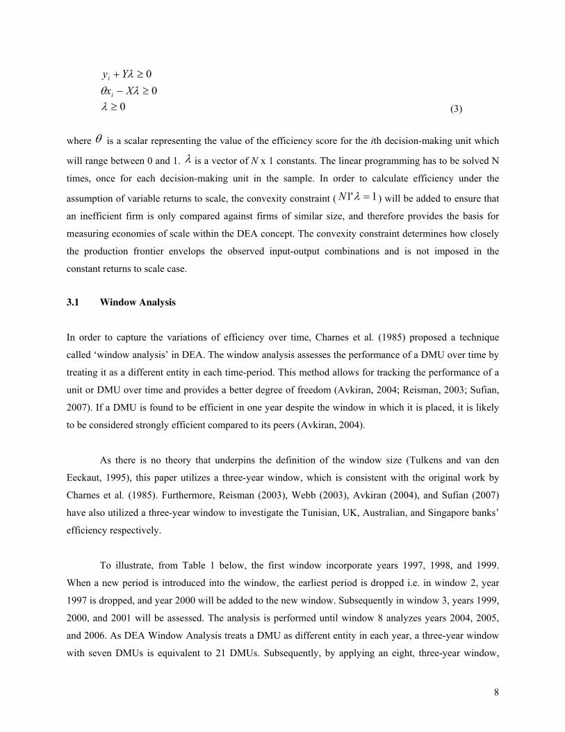
0≥+ λYyi

0≥− λθ Xxi

0≥λ (3)

where θ is a scalar representing the value of the efficiency score for the ith decision-making unit which

will range between 0 and 1. λ is a vector of N x 1 constants. The linear programming has to be solved N

times, once for each decision-making unit in the sample. In order to calculate efficiency under the

assumption of variable returns to scale, the convexity constraint ( 1'1 =λN ) will be added to ensure that

an inefficient firm is only compared against firms of similar size, and therefore provides the basis for

measuring economies of scale within the DEA concept. The convexity constraint determines how closely

the production frontier envelops the observed input-output combinations and is not imposed in the

constant returns to scale case.

3.1 Window Analysis

In order to capture the variations of efficiency over time, Charnes et al. (1985) proposed a technique

called ‘window analysis’ in DEA. The window analysis assesses the performance of a DMU over time by

treating it as a different entity in each time-period. This method allows for tracking the performance of a

unit or DMU over time and provides a better degree of freedom (Avkiran, 2004; Reisman, 2003; Sufian,

2007). If a DMU is found to be efficient in one year despite the window in which it is placed, it is likely

to be considered strongly efficient compared to its peers (Avkiran, 2004).

As there is no theory that underpins the definition of the window size (Tulkens and van den

Eeckaut, 1995), this paper utilizes a three-year window, which is consistent with the original work by

Charnes et al. (1985). Furthermore, Reisman (2003), Webb (2003), Avkiran (2004), and Sufian (2007)

have also utilized a three-year window to investigate the Tunisian, UK, Australian, and Singapore banks’

efficiency respectively.

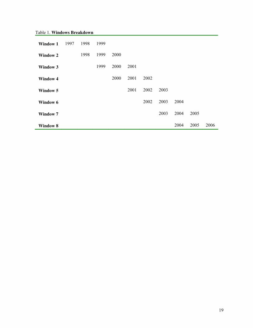
To illustrate, from Table 1 below, the first window incorporate years 1997, 1998, and 1999.

When a new period is introduced into the window, the earliest period is dropped i.e. in window 2, year

1997 is dropped, and year 2000 will be added to the new window. Subsequently in window 3, years 1999,

2000, and 2001 will be assessed. The analysis is performed until window 8 analyzes years 2004, 2005,

and 2006. As DEA Window Analysis treats a DMU as different entity in each year, a three-year window

with seven DMUs is equivalent to 21 DMUs. Subsequently, by applying an eight, three-year window,

9

would considerably increase the number of observations of the sample to 168 (i.e. 7x3x8), thus providing

a greater degree of freedom to the sample4.

[Insert Table 1]

3.2 Linking Bank Efficiency to Share Price Returns

Given the unbalanced nature of the panel, several econometric issues arise. In order to examine the

relationship between China bank efficiency and its share price performance, several specification tests are

performed. First, although banks may be modelled as potentially heterogeneous cross-sectional units,

estimations are conducted assuming homogeneity. This approach is justified on the assumption that

parameters are homogeneous across banks. Furthermore, Baltagi et al. (2003) argues that when the

sample is short, homogeneous panel estimation may be a more preferred approach to heterogeneous panel

estimation.

Another issue concerns what estimation approach to use between pooled analysis, fixed effects

and/or random effects. To determine the choice of the appropriate methodology, following the procedures

set in Baltagi (2001), several specification tests are employed. To choose between fixed effects and

pooled estimation, the likelihood ratio (LR) test was used and the Breush-Pagan Lagrange Multiplier

(LM) test was conducted to assess whether the model must be estimated by random effects or pooled

estimation analysis, while the Hausman test was used to choose between fixed and random effects. In all

the specifications, pooled analysis was rejected at conventional significance level. In a majority of

specifications, the Hausman test urges the use of fixed effects estimation. Accordingly, in order to

account for unobserved factors, the empirical evidence presented in the paper is based on the fixed effects

estimation.

The relationship between bank efficiency and share price performance is examined by regressing

bank share returns against bank efficiency estimates derived from the DEA Window Analysis method. In

addition to the basic pooled OLS model, this paper estimates panel regression method by combining cross

section and time series data with the fixed effect estimators to control for the heterogeneity among bank

specific factors, which are not considered in the basic regression model that may affect share price return,

knowingly or not. White’s (1980) heteroscedasticity consistent statistics is used. Accordingly, the

following model is estimated:

4 Due to entry and exit, the total number of bank year observations total 127.

10

SHR_RETjt = α0 + βEFFjt + βΣBSFjt + ∈j (4)

jtjjt νμε +=

where SHR_RETjt is the moving average of bank j’s daily share returns in window t; α0 are bank j’s fixed

effects, EFFjt is bank j’s mean annual percentage change in bank efficiency in window t; β are the

parameters to be estimated excluding the constant; and ∈j is a normally distributed error term. The error

term is assumed to be free from autocorrelation. Heteroskedasticity is corrected in the estimations by

using the robust variance covariance matrix.

EFFjt include the technical, pure technical, and scale efficiency scores derived from the DEA

Window Analysis method. BSFjt is an array of bank specific factors that are relevant to the modern

banking business. These include LNDEPO as a proxy of bank’s market power calculated as a natural

logarithm of total bank deposits. LOANTA is a measure of bank’s loans intensity calculated as the ratio of

total loans to bank total assets. LNTA is the size of the bank’s total asset measured as the natural

logarithm of banks’ total assets. NIE/TA is a measure of bank management quality calculated as total non-

interest expenses divided by total assets. NII/TA is a measure of bank’s diversification towards non-

interest income, calculated as total non-interest income divided by total assets. EQUITY/TA is a measure

of banks’ leverage intensity measured by banks’ total shareholders equity divided by total assets. ROA is

a proxy measure for bank profitability calculated as bank profit after tax divided by total assets. Finally,

INV/TA is a proxy measure for investment capacity calculated as investment divided by total assets.

3.3 Variables Definition

In the banking theory literature, there are two main approaches competing with each other in this regard;

the production and intermediation approaches (Sealey and Lindley, 1977). Under the production approach

pioneered by Benston (1965), a financial institution is defined as a producer of services for account

holders, that is, they perform transactions on deposit accounts and process documents such as loans. The

intermediation approach on the other hand assumes that financial firms act as an intermediary between

savers and borrowers and posits total loans and securities as outputs, whereas deposits along with labour

and physical capital are defined as inputs.

For the purpose of this study, a variation of the intermediation approach or asset approach

originally developed by Sealey and Lindley (1977) is adopted in the definition of inputs and outputs used.

According to Berger and Humphrey (1997), the production approach might be more suitable for branch

11

efficiency studies as at most times bank branches process customer documents and bank funding, while

investment decisions are mostly not under the control of branches. Accordingly, we model China

commercial banking groups as multi-product firms, producing two outputs by employing two inputs. All

variables are measured in million of China Renminbi (RMB). This study employs annual data from 1997

to 2006 for each of the state-owned and joint stock commercial banks listed on the Shanghai Stock

Exchange. All of the data come from of the Almanac of China’s Finance and Banking (various editions).

The input vectors include (x1) Total Deposits, which includes deposits from customers and other

banks and (x2) Fixed Assets while (y1) Total Loans, which includes loans to customers and other banks

and (y2) Investments are the output vectors. Table 2 presents the descriptive statistics for the selected

variables that are categorized under the intermediation approach of modelling bank behaviour.

[Insert Table 2]

For the panel regression analysis, individual banks’ annual share returns are obtained from

Bloomberg. The annual share returns are calculated as the sum of daily share returns for all listed China

banks namely, China Merchants Bank Co Ltd (CMB), China Minsheng Banking Corporation (CHMB),

Hua Xia Bank (HXB), Industrial and Commercial Bank of China (ICBC), Industrial Bank Co Ltd (IBC),

Shanghai Pudong Development Bank (SPDB), and Shenzhen Development Bank Co. Ltd (SDB). This

measure is believed to be a better measure than calculating a point increase with data from the first and

the last day of the period under investigation. Daily returns have smaller standard deviations than do

annual and monthly returns5.

4. EMPIRICAL RESULTS

As mentioned earlier, this study will be the first to examine the efficiency of the China banking sector by

utilizing the DEA Window Analysis method. To recap, the DEA model is applied to eight, three-year

windows, and the results are reported for the general trends in technical efficiency for each window

before we embark to briefly discuss the decomposition of technical efficiency into its mutually exhaustive

pure technical and scale efficiency components. Changes over time for the sequence of the windows are

then considered.

5 The mean standard deviation of monthly returns for randomly selected securities is about 7.8%, while the corresponding mean standard

deviation of daily returns will be approximately 1.8% if daily returns are serially independent (Fama, 1976, pp.123).

12

The average of all scores for each bank is given in the column denoted ‘Mean’. The column

labeled ‘SD’ indicates the standard deviation for the score of each bank during the entire period. The

column labeled ‘LDY’ indicates the largest difference in a bank’s scores in the same year but in different

windows. The column labeled ‘LDP’ indicates the largest difference in a bank’s scores for the entire

period. A bank can have different efficiency scores in different windows. A bank that is efficient in one

year regardless of the window is said to be stable in its efficiency rating (Cooper et al. 2000).

4.1 Efficiency of the China Banking Sector

Table 3 presents the decomposition of the technical efficiency scores for each bank, with each bank

represented as if it is a different DMU at each of the three successive dates noted at the top of each

column. Eight separate windows are presented as separate rows in Table 3. Taking CHMB for example,

in Table 3, the technical efficiency of CHMB in the first window is 81.9%, 100.0%, and 98.3%. These

figures correspond to the estimated relative efficiency of CHMB for years 1997, 1998, and 1999

respectively. In the second window, the relative efficiency estimates of 100.0%, 95.2%, and 100.0%

correspond to years 1998, 1999, and 2000 respectively.

The approach used in formulating Table 3 lends itself to a study of ‘trends’ and the examination

of the ‘stability’ of efficiency scores, as well as within windows by the adoption of ‘row views’ and

‘column views’ respectively. For instance, taking CHMB again for example, the bank’s efficiency varies

from 85.6% to 100.0% in years 2000 through to 2002 (window 4) by adopting a ‘row view’ perspective.

At the same time, the efficiency of a DMU within different windows can also vary substantially by

adopting a ‘column view’ perspective. This variation reflects simultaneously both the absolute

performance of a bank over time and the relative performance of that bank in comparison to its peers in

the sample.

[Insert Table 3]

It is observed from Table 3 that SDB is the most efficient bank during the period, maintaining its

position with mean technical efficiency of 96.5% and accompanied by a relatively low standard

deviations of 0.052, which is consistent with Charnes et al. (1985). To recap, Charnes et al. (1985)

suggested that DMUs with high efficiency levels tend to demonstrate lower standard deviations compared

to its peers with lower efficiency levels. While SDB is the most efficient bank in terms of minimizing

costs to produce the same level of outputs, on the other hand the findings seem to suggest that HXB is the

13

least efficient bank with a mean technical efficiency level of 81.6% and standard deviation of 0.087

during the period of study.

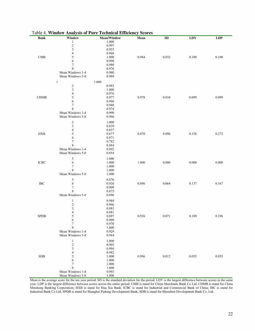
Table 4 presents the results for the pure technical efficiency of the China banks. In general, it has

been concluded by Berger et al. (1993) that large banks tend to report higher levels of pure technical

efficiency than do their smaller counterparts. Supporting the findings of Berger et al. (1993), we find that

the large banks namely, HXB, ICBC, and IBC have reported the highest mean pure technical efficiency of

98.2%, followed by the small banks, CHMB and SDB, with a mean pure technical efficiency of 94.0%,

while the medium banking groups, SPDB and CMB, with total assets ranging from RMB50 billion to

RMB100 billion, have reported the lowest mean pure technical efficiency of 93.9%.

[Insert Table 4]

It could be argued that the large banks may have the advantage over its smaller counterparts as

the large banks may attract more deposits and loan transactions and in the process, command larger

interest rate spreads. Furthermore, large banks may offer more services and in the process derive

substantial non-interest income from commissions, fees and other treasury activities. Randhawa and Lim

(2005) find that the large banks’ extensive branch networks and large depositor base have attracted

cheaper source of funds. On the other hand, the smaller banking groups with smaller depositor base might

have to resort to purchasing funds in the inter-bank market, which is costlier.

It is worth mentioning that earlier bank efficiency studies have generally found large banks tend

to report lower level of scale efficiency (Miller and Noulas, 1996; Drake and Hall, 2003; Webb, 2003).

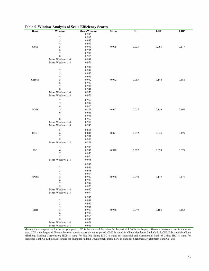
Similar to the pure technical efficiency results, it is clear from Table 5 that the small China banks have

exhibited the lowest mean scale efficiency compared to its medium and large counterparts. The findings

seem to suggest that the small banks namely, CHMB and SDB have reported the lowest mean scale

efficiency of 95.6% compared to their large bank counterparts namely, HXB, ICBC, and IBC, with total

assets of over RMB100 billion, which have exhibited mean scale efficiency of 95.9%. On the other hand,

the results seem to suggest that the medium sized banks have exhibited the highest mean scale efficiency

of 97.9% during the period of study.

[Insert Table 5]

14

4.2 Efficiency and China Banks’ Share Price Returns

Share price performance could be argued to be the ultimate measure of efficiency. If bank share prices

reflect almost all the information about the past, present, and expected future performance of firms, then

this measure would be the more reliable indicator of bank efficiency. However, even if the choice of

measures is correct, the previously described measures of efficiency may only be related to share price

performance in the long-term. Short-term variations may not be explained by efficiency measures. In this

case, individual bank effects may explain the majority of total variations in share price performance. In

term of average share price performance over the years, CHMB has exhibited the highest annual share

return of 37.86%, while SDB exhibited the lowest average annual share return of 1.47% over the sample

period. In terms of share returns volatility, CHMB share price was the most volatile, while HXB was the

most stable6.

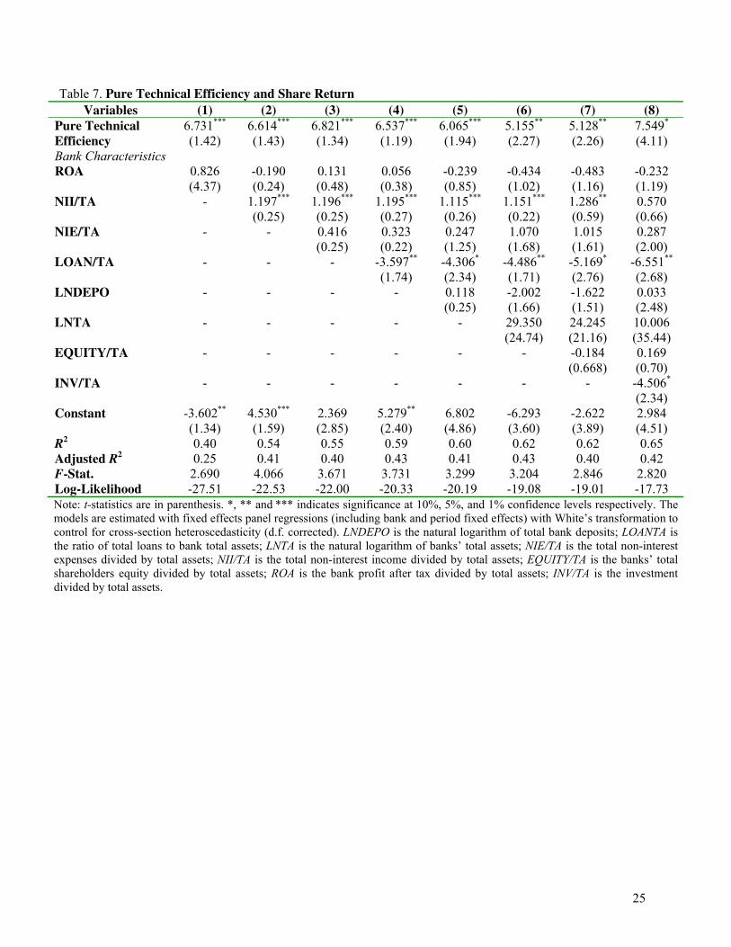
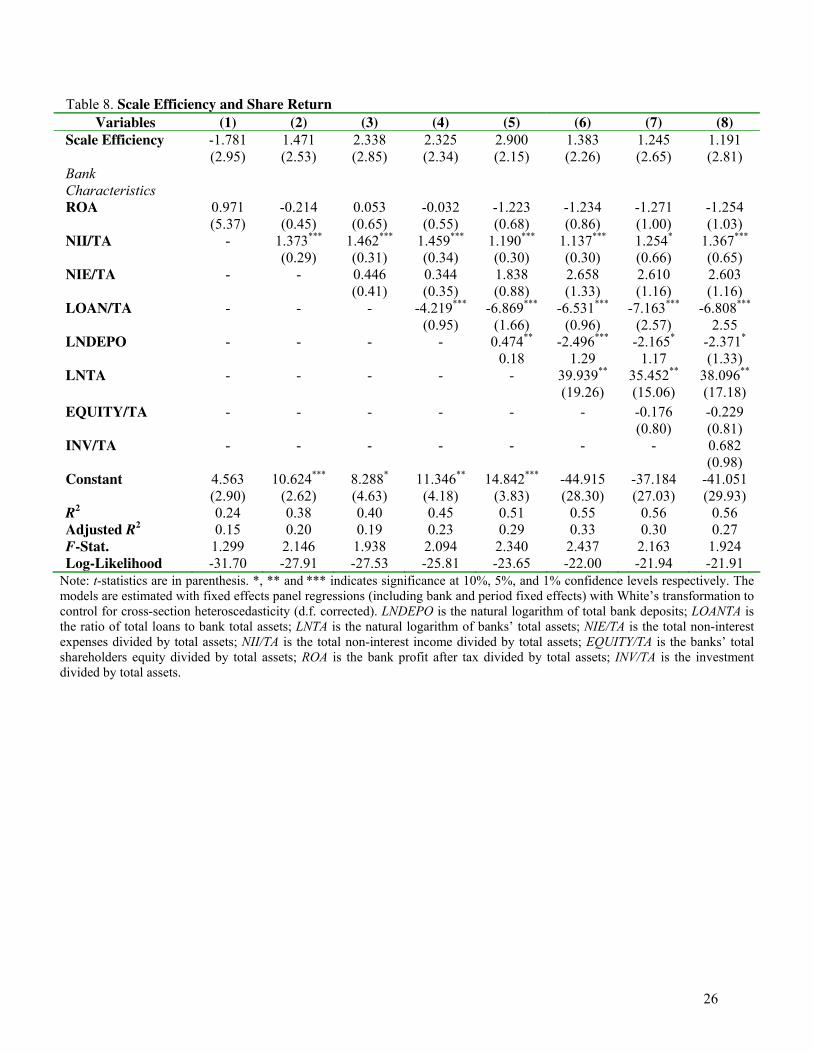
To examine whether statistical relationship exists between bank efficiency scores derived from

the DEA Window Analysis method and China banks’ share price performance, Equation (4) is estimated

by using bank efficiency scores as the independent variable against share price return as the dependent

variable. It is expected that the efficiency scores to be positively correlated with share prices. Tables 6-8

present the results derived from estimating Equation (4) by panel regression model with fixed-effects. It is

interesting to note that the results from the fixed-effect model continued to remain robust across various

regressions models with the inclusion of other bank specific trait variables. This gives us comfort into that

accurate inferences are made regarding the test results.

Regression results focusing on the relationship between bank efficiency and share prices and

other explanatory variables are presented in Tables 6-8. It is observed that both TE and PTE entered the

regression models positively and significantly as expected. However, the coefficient of SE is insignificant

in any of the regression models. These findings suggest that share prices of the relatively more

managerially efficient banks tend to outperform their inefficient counterparts, which is consistent with

earlier studies by among others Chu and Lim (1998), Beccalli et al. (2006), and Sufian and Majid (2006).

On the other hand, the empirical findings seem to suggest that scale efficiency does not explain the

variations in share prices in the marketplace. It is observed from Tables 6-8, the inclusion of other

explanatory variables in Models 2-8 increase the explanatory power of the regression models with the

variation in share price return ranges between 25% – 65% (adjusted variation is between 15% – 43%).

6 For brevity purposes, the table has been excluded from the text but is available from the authors upon request.

15

This indicates that the inclusion of other bank specific traits in the regression models to contribute to a

better goodness of fit in explaining the variation in share price performance.

[Insert Table 6-8]

To further analyze this relationship, the reaction of changes in different bank efficiency estimates

on share price returns is further examined by the magnitudes of the coefficient derived from the panel

regression model. The magnitude of the coefficient of technical efficiency scores are positive ranging

between 2.21 – 5.39, implying that a one percent improvement in efficiency would lead to the

improvement in China banks’ share prices between 2.21% – 5.39%. Likewise, the magnitude of the

coefficient of pure technical efficiency scores is also positive, albeit higher, ranging between 5.12 – 7.55.

On the other hand, China banks’ share price returns seem not to react to changes in scale efficiency. The

empirical findings seem to suggest that share price returns respond positively towards improvement in

managerial efficiency but do not react towards changes in scale efficiency. The empirical results

presented in this paper also concur with the earlier findings by Pasiouras et al. (2008) on the Greece

banking sector, who suggest that changes in scale efficiency have no impact on share price performance.

Another important result of the regression models is the significance of the relationship between

banks’ share price returns and TE, PTE, and other bank specific trait variables namely, NII/TA, LOAN/TA,

and INV/TA across all regression models. Nevertheless, the relationship between share price returns, SE,

and other bank trait variables namely, NII/TA, NIE/TA, LOAN/TA, LNDEPO, and LNTA also contribute to

better understanding on the variation of China banks’ share price behaviour. The coefficient of NII/TA

entered the regression models positively, suggesting that higher income from non-interest based product

enhances share price performance. The coefficient of the variable LOAN/TA has a negative effect on share

price returns, suggesting that banks with a higher level of loans-to-asset ratio could have a riskier loan

portfolio and therefore, negatively affecting banks’ income.

The coefficient of the INV/TA variable is negative and is statistically significant, indicating that

banks, which do not maximize its investment capacity, will not improve their share price performance.

The coefficient of LNTA exhibits a positive sign, implying that larger banks are more efficient in

minimizing their operating costs. On the other hand, LNDEPO entered the regression models negatively.

Finally, NIE/TA exhibits a positive sign implying that better management’s technical ability in managing

their operating costs would lead to higher earnings, which would translate into higher share price returns.

16

5. CONCLUSIONS

The paper attempts to investigate the efficiency of listed China commercial banks during the

period of 1997-2006. The preferred non-parametric DEA Window Analysis methodology allows us to

distinguish between three different types of efficiency, namely the technical, pure technical, and scale

efficiency. In addition, the method also provides greater degree of freedom to the sample.

Our findings are consistent with prior evidence in the existing literature on bank efficiency

(Berger et al. 1993) that large banks tend to report higher levels of pure technical efficiency, than do their

smaller counterparts. The empirical findings suggest that large China banks have exhibited higher

technical and pure technical efficiency levels compared to their small and medium sized bank

counterparts. On the other hand, the medium sized banks have exhibited a higher scale efficiency

compared to their small and large bank peers.

The explanation of the efficiency scores using panel regressions offers useful economic insights.

Bank efficiency is found to be related to bank characteristics. Bank efficiency is found to decline with

investment capacity, loans intensity, and market power, while it is found to increase with bank

management quality, size, and bank’s diversification towards non-interest income. Furthermore, the

results suggest that changes in technical efficiency are statistically significant in determining banks’ share

price returns, whereas scale efficiency does not explain the variation in share price returns. The most

important finding here would be that the efficiency of a bank’s operation has significant information

about its share price performance, which is not explained by market movements.

One implication of the findings is that managerially efficient banks, ceteris paribus, should be

more profitable and therefore generates greater shareholder returns7. This is in line with the efficient

market theory that in an efficient market a change in cost efficiency should be incorporated in the price

formation process. Nevertheless, generalization of this conclusion would require more studies involving

the whole range of industries and the banking sector.

7 As pointed out by Eisenbeis et al. (1999) the ceteris paribus condition is important since cost is only one half of the profit equation and

therefore does not tell the full story. For example, a bank may offer greater customer services, which while more costly, also increases revenues.

17

REFERENCES

Adenso-Diaz, B. and Gascon, F. (1997), Linking and Weighting Efficiency Estimates with Stock

Performance in Banking Firms, Working Paper, Wharton Financial Institutions Centre.

Ariff, M. and Can, L. (2007), Cost and Profit Efficiency of Chinese Banks: A Non-Parametric Analysis,

China Economic Review (2007), doi: 10.1016/j.chieco.2007.04.001.

Avkiran, N.K. (2004), Decomposing Technical Efficiency and Window Analysis, Studies in Economics

and Finance 22 (1), 61-91.

Ball, R. and Kothari, S.P. (1994), Financial Statement Analysis. New York, NY: Mc-Graw Hill.

Baltagi, B. (2001), Econometric Analysis of Panel Data. New York, NY: John Wiley.

Baltagi, D., Bresson, G., Griffin, J. and Pirote, A. (2003). Homogeneous, Heterogenous or Shrinkage

Estimators? Some Empirical Evidence from French Regional Gasoline Consumption, Empirical

Economics 28, 795-811.

Beccalli, E., Casu, B. and Girardone, C. (2006), Efficiency and Stock Performance in European Banking,

Journal of Business Finance and Accounting 33, 245-262

Benston, G.J. (1965), Branch Banking and Economies of Scale, Journal of Finance 20 (2), 312-331.

Berger A.N., Hasan, I. and Zhou, M. (2007), Bank Ownership and Efficiency in China: What Will

Happen in the World’s Largest Nation, Working Paper Wharton Financial Institutions Center.

Berger, A. N., Hunter, W. C. and Timme, S. G. (1993), The Efficiency of Financial Institutions: A

Review and Preview of Research Past, Present and Future,’ Journal of Banking and Finance 17 (2-3),

221-249.

Berger, A.N. and Humphrey, D.B. (1997), Efficiency of Financial Institutions: International Survey and

Directions for Future Research, European Journal of Operational Research 98 (2), 175-212.

Brealey, R.A. and Myers, S.C. (1991), Principles of Corporate Finance. New York, NY: Mc-Graw Hill.

Charnes, A., Clark, C.T., Cooper W.W. and Golany, B. (1985), A Developmental Study of Data

Envelopment Analysis in Measuring the Efficiency of Maintenance Units in the U.S. Air Forces, Annals

of Operations Research 2 (1), 95 –112.

Chen, X., Skully, M. and Brown, K. (2005), Banking Efficiency in China: Application of DEA to Pre-

and Post-Deregulation Eras: 1993–2000, China Economic Review 16, 229–245.

Chen, X., Skully, M. and Brown, K. (2005), Banking Efficiency in China: An Application of DEA to Pre-

and Post Deregulation Era: 1993-2000, China Economic Review 16, 229-245.

China Finance Society (various issues), Almanac of China’s Finance and Banking (Annual), Beijing:

China Financial Publishing House.

Chu, S.F. and Lim, G.H. (1998), Share Performance and Profit Efficiency of Banks in an Oligopolistic

Market: Evidence from Singapore, Journal of Multinational Financial Management 8 (2-3), 155-168.

Coelli, T. (1996), A Guide to DEAP Version 2.1: A Data Envelopment Analysis (Computer Program),

Working Paper, CEPA, University of New England, Armidale.

Coelli, T., Prasada-Rao, D.S. and Battese, G.E. (1998), An Introduction to Efficiency and Productivity

Analysis. Boston: Kluwer Academic Publishers.

Cooper, W.W., Seiford. L.M. and Tone, K. (2000), Data Envelopment Analysis: A Comprehensive Text

with Models, Applications, References and DEA-Solver Software. Boston: Kluwer Academic Publishers. Drake, L. and Hall, M.J.B. (2003), Efficiency in Japanese Banking: An Empirical Analysis, Journal of

Banking and Finance 27, 891-917.

Eisenbeis, R.A., Ferrier, G.D. and Kwan, S.H. (1999), The Informativeness of Stochastic Frontier and

Programming Frontier Efficiency Scores: Cost Efficiency and Other Measures of Bank Holding Company

Performance, Working Paper Federal Reserve Bank of Atlanta.

Elyasiani, E. and Mehdian, S. (1992), Productive Efficiency Performance of Minority and Non-Minority

Owned Banks: A Non-Parametric Approach, Journal of Banking and Finance 16 (5), 933-948.

Fama, E.F. (1976). Foundations of Finance, Basic Books.

Fu, X. and Heffernan, S. (2007), Cost X-efficiency in China's Banking Sector, China Economic Review

18, 35–53.

18

Hsiao, C. (1985), Benefits and Limitations of Panel Data, Econometric Review 4, 121-174.

Kirkwood, J. and Nahm, D. (2006), Australian Banking Efficiency and Its Relation to Stock Returns, The

Economic Record 82, 253-267.

Kothari, S.P. (2001), Capital Markets Research in Accounting, Journal of Accounting and Economics 31,

105-231.

Liu, C. and Song, W. (2004), Efficiency Analysis in China Commercial Banks Based on SFA, Journal of

Financial Research 6, 138-142 (in Chinese)

Miller, S.M. and Noulas, A.G. (1996), The Technical Efficiency of Large Bank Production, Journal of

Banking and Finance, 20 (3): 495-509.

Pasiouras, F. Liadaki, A. and Zopounidis, C. (2007), Bank Efficiency and Share Performance: Evidence

from Greece, Forthcoming in Applied Financial Economics.

Qian, Q. (2003), On the Efficiency Analysis of SFA in China Commercial Banks, Social Science of

Nanjing 1, 41-46 (in Chinese)

Qing, W. and Ou, Y. (2001), Chinese Commercial Banks: Market Structure, Efficiency, and its

Performance, Economic Science 100871, 34-45 (in Chinese).

Randhawa, D.S. and Lim, G.H. (2005), Competition, Liberalization and Efficiency: Evidence from a Two

Stage Banking Models on Banks in Hong Kong and Singapore, Managerial Finance 31 (1), 52-77.

Reisman, A., Daouas, M., Oral, M., Rebai, S. and Gatoufi, S. (2003), Impact of Deregulation on

Technical and Scale Efficiencies of Tunisian Commercial Banks: Window Extended Data Envelopment

Analysis, Working Paper, Faculte des Sciences Economiques et de Gestion de Tunis, Universite El

Manar, Tunisie.

Sealey, C. and Lindley, J.T. (1977), Inputs, Outputs and a Theory of Production and Cost at Depository

Financial Institutions, Journal of Finance 32 (4), 1251-1266.

Sufian, F. (2007), Trends in the Efficiency of Singapore’s Commercial Banking Groups: A Non-

Stochastic Frontier DEA Window Analysis Approach, International Journal of Productivity and

Performance Management 56 (2), 99-136.

Sufian, F. and Majid, A.M.Z. (2006), Banks Efficiency and Stock Prices in Emerging Market: Evidence

from Malaysia, Journal of Asia-Pacific and Business 7 (4), 35-53.

Thanassoulis, E. (2001), Introduction to the Theory and Application of Data Envelopment Analysis: A

Foundation Text with Integrated Software. Boston: Kluwer Academic Publishers.

Tulkens, H. and van den Eeckaut, P. (1995), Nonparametric Efficiency, Progress and Regress Measures

for Panel Data: Methodological Aspects, European Journal of Operational Research 80 (3), 474-499.

Webb, R.W. (2003), Levels of Efficiency in UK Retail Banks: A DEA Window Analysis, International

Journal of the Economics of Business 10 (3), 305-322.

Wei, Y. and Wang, L. (2000), The Non-Parametric Approach to the Measurement of Efficiency: The

Case of China Commercial Banks, Journal of Financial Research 3, 88-96 (in Chinese). White, H. J. (1980), A Heteroskedasticity-Consistent Covariance Matrix Estimator and a Direct Test for

Heteroskedasticity, Econometrica 48 (4), 817-838.

Xu, Z., Junmin, Z. and Zhenseng, J. (2001), An Analysis of the Efficiency of State Owned Banks with

Examples, South China Financial Research 16 (1), 25-27 (in Chinese)

Xue, F. and Yang, D. (1998), Evaluating Bank Management and Efficiency Using the DEA Model,

Econometrics and Technological Economy Research 6, 63-66 (in Chinese)

Yao, S., Jiang, C., Feng G., and Willenbockel, D. (2007), On the Efficiency of Chinese Banks and WTO

Challenges, Applied Economics 39 (5), 629-43.

Zhang, C., Gu, F. and Di, Q. (2005), Cost Efficiency Measurement in China Commercial Banks Based on

Stochastic Frontier Analysis, Explorations in Economic Issues 6, 116-119 (in Chinese)

Zhao, X. (2000), State Owned Commercial Banks Efficiency Analysis, Journal of Economic Science 6,

45-50 (in Chinese)

19

Table 1. Windows Breakdown

Window 1

1997

1998

1999

Window 2

1998

1999

2000

Window 3

1999

2000

2001

Window 4

2000

2001

2002

Window 5

2001

2002

2003

Window 6

2002

2003

2004

Window 7

2003

2004

2005

Window 8

2004

2005

2006

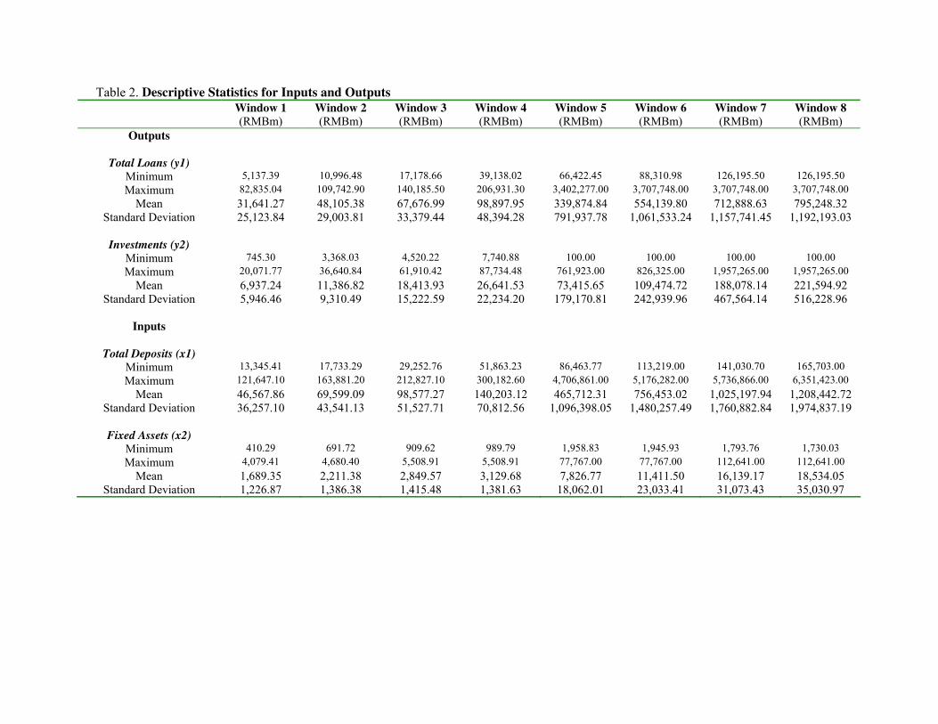
Table 2. Descriptive Statistics for Inputs and Outputs

Window 1

(RMBm) Window 2

(RMBm) Window 3

(RMBm) Window 4

(RMBm) Window 5

(RMBm) Window 6

(RMBm) Window 7

(RMBm) Window 8

(RMBm)

Outputs

Total Loans (y1)

Minimum 5,137.39 10,996.48 17,178.66 39,138.02 66,422.45 88,310.98 126,195.50 126,195.50

Maximum 82,835.04 109,742.90 140,185.50 206,931.30 3,402,277.00 3,707,748.00 3,707,748.00 3,707,748.00

Mean 31,641.27 48,105.38 67,676.99 98,897.95 339,874.84 554,139.80 712,888.63 795,248.32

Standard Deviation 25,123.84 29,003.81 33,379.44 48,394.28 791,937.78 1,061,533.24 1,157,741.45 1,192,193.03

Investments (y2)

Minimum 745.30 3,368.03 4,520.22 7,740.88 100.00 100.00 100.00 100.00

Maximum 20,071.77 36,640.84 61,910.42 87,734.48 761,923.00 826,325.00 1,957,265.00 1,957,265.00

Mean 6,937.24 11,386.82 18,413.93 26,641.53 73,415.65 109,474.72 188,078.14 221,594.92

Standard Deviation 5,946.46 9,310.49 15,222.59 22,234.20 179,170.81 242,939.96 467,564.14 516,228.96

Inputs

Total Deposits (x1)

Minimum 13,345.41 17,733.29 29,252.76 51,863.23 86,463.77 113,219.00 141,030.70 165,703.00

Maximum 121,647.10 163,881.20 212,827.10 300,182.60 4,706,861.00 5,176,282.00 5,736,866.00 6,351,423.00

Mean 46,567.86 69,599.09 98,577.27 140,203.12 465,712.31 756,453.02 1,025,197.94 1,208,442.72

Standard Deviation 36,257.10 43,541.13 51,527.71 70,812.56 1,096,398.05 1,480,257.49 1,760,882.84 1,974,837.19

Fixed Assets (x2)

Minimum 410.29 691.72 909.62 989.79 1,958.83 1,945.93 1,793.76 1,730.03

Maximum 4,079.41 4,680.40 5,508.91 5,508.91 77,767.00 77,767.00 112,641.00 112,641.00

Mean 1,689.35 2,211.38 2,849.57 3,129.68 7,826.77 11,411.50 16,139.17 18,534.05

Standard Deviation 1,226.87 1,386.38 1,415.48 1,381.63 18,062.01 23,033.41 31,073.43 35,030.97

21

Table 3. Window Analysis of Technical Efficiency Scores Bank Window Mean/Window Mean SD LDY LDP

1 0.985

2 0.964

3 0.938

4 0.958

CMB 5 0.999 0.960 0.048 0.120 0.120

6 0.983

7 0.960

8 0.892

Mean Windows 1-4 0.962


1 0.934

2 0.984

3 0.952

4 0.913

CHMB 5 0.930 0.941 0.059 0.144 0.181

6 0.954

7 0.946

8 0.915



2 0.952

3 0.829

4 0.766

HXB 5 0.762 0.816 0.087 0.205 0.299

6 0.771

7 0.779

8 0.853



5 0.836

ICBC 6 0.846 0.871 0.072 0.045 0.199

7 0.901

8 0.900


5 0.863

IBC 6 0.924 0.882 0.060 0.147 0.173

7 0.888

8 0.851


1 0.976

2 0.934

3 0.862

4 0.801

SPDB 5 0.839 0.906 0.081 0.128 0.232

6 0.900

7 0.964

8 0.975



1 0.997

2 0.995

3 0.954

4 0.909

SDB 5 0.963 0.964 0.052 0.163 0.163

6 0.989

7 0.965

8 0.942



Mean is the average score for the ten year period; SD is the standard deviation for the period; LDY is the largest difference between scores in the same

year; LDP is the largest difference between scores across the entire period. CMB is stand for China Merchants Bank Co Ltd; CHMB is stand for China

Minsheng Banking Corporation; HXB is stand for Hua Xia Bank; ICBC is stand for Industrial and Commercial Bank of China; IBC is stand for

Industrial Bank Co Ltd; SPDB is stand for Shanghai Pudong Development Bank; SDB is stand for Shenzhen Development Bank Co. Ltd.

22

Table 4. Window Analysis of Pure Technical Efficiency Scores Bank Window Mean/Window Mean SD LDY LDP

1 1.000

2 0.997

3 0.955

4 0.968

CMB 5 1.000 0.984 0.032 0.100 0.100

6 0.998

7 0.980

8 0.976



1 1.000

2 0.985

3 1.000

4 0.976

CHMB 5 0.977 0.978 0.034 0.099 0.099

6 0.966

7 0.948

8 0.974



2 1.000

3 0.839

4 0.837

HXB 5 0.877 0.870 0.096 0.158 0.272

6 0.871

7 0.782

8 0.884



5 1.000

ICBC 6 1.000 1.000 0.000 0.000 0.000

7 1.000

8 1.000


5 0.876

IBC 6 0.926 0.896 0.064 0.137 0.167

7 0.909

8 0.875


1 0.984

2 0.966

3 0.883

4 0.881

SPDB 5 0.897 0.936 0.071 0.189 0.196

6 0.909

7 0.970

8 1.000



1 1.000

2 0.995

3 0.994

4 0.982

SDB 5 1.000 0.996 0.012 0.055 0.055

6 1.000

7 1.000

8 1.000







23

Table 5. Window Analysis of Scale Efficiency Scores Bank Window Mean/Window Mean SD LDY LDP

1 0.985

2 0.967

3 0.983

4 0.990

CMB 5 0.999 0.975 0.033 0.061 0.117

6 0.985

7 0.980

8 0.915



1 0.934

2 0.999

3 0.952

4 0.936

CHMB 5 0.952 0.962 0.055 0.144 0.181

6 0.987

7 0.998

8 0.941



2 0.952

3 0.988

4 0.915

HXB 5 0.871 0.947 0.057 0.153 0.161

6 0.945

7 0.996

8 0.962



5 0.836

ICBC 6 0.846 0.871 0.072 0.045 0.199

7 0.901

8 0.900


5 0.985

IBC 6 0.997 0.978 0.027 0.078 0.078

7 0.955

8 0.974


1 0.992

2 0.966

3 0.978

4 0.914

SPDB 5 0.937 0.968 0.040 0.147 0.170

6 0.989

7 0.994

8 0.975



1 0.997

2 0.999

3 0.960

4 0.926

SDB 5 0.963 0.968 0.049 0.163 0.163

6 0.989

7 0.965

8 0.942







24

Table 6. Technical Efficiency and Share Return

Variables (1) (2) (3) (4) (5) (6) (7) (8)

Technical Efficiency 2.207

(1.57)

4.353***

(1.12)

5.380***

(1.35)

5.192***

(1.28)

4.713***

(1.36)

4.025***

(1.46)

4.018**

(1.54)

5.390**

(2.33)

Bank Characteristics

ROA -0.906

(5.98)

-0.555

(0.39)

-0.019

(0.73)

-0.091

(0.66)

-0.700

(0.90)

-0.800

(0.98)

-0.803

(1.08)

-0.735

(1.14)

NII/TA - 1.655***

(0.32)

1.756***

(0.30)

1.736***

(0.32)

1.514***

(0.24)

1.470***

(0.23)

1.479***

(0.54)

0.994*

(0.55)

NIE/TA - - 0.832*

(0.43)

0.723*

(0.39)

0.510

(1.06)

1.088

(1.41)

1.087

(1.41)

0.589

(1.63)

LOAN/TA - - - -3.724**

(1.44)

-5.173***

(1.81)

-5.279***

(1.54)

-5.327**

(2.29)

-6.484**

(2.34)

LNDEPO - - - - 0.251

(0.18)

-1.134

(1.28)

-1.111

(1.23)

0.317

(2.03)

LNTA - - - - - 19.119

(18.83)

18.807

(16.67)

10.579

(27.77)

EQUITY/TA - - - - - - -0.012

(0.63)

0.316

(0.60)

INV/TA - - - - - - - -3.455**

(1.67)

Constant 0.802

(1.51)

2.505***

(3.95)

5.732

(4.53)

8.567*

(4.38)

11.021**

(4.93)

-17.200

(27.44)

-16.658

(26.26)

10.289

(40.75)

R2 0.26 0.50 0.55 0.59 0.61 0.62 0.62 0.63

Adjusted R2 0.18 0.36 0.40 0.43 0.43 0.42 0.39 0.39

F-Stat. 1.472 3.503 3.611 3.714 3.469 3.160 2.790 2.656

Log-Likelihood -31.13 -23.95 -22.17 -20.38 -19.64 -19.23 -19.23 -18.42

Note: t-statistics are in parenthesis. *, ** and *** indicates significance at 10%, 5%, and 1% confidence levels respectively. The

models are estimated with fixed effects panel regressions (including bank and period fixed effects) with White’s transformation to

control for cross-section heteroscedasticity (d.f. corrected). LNDEPO is the natural logarithm of total bank deposits; LOANTA is the

ratio of total loans to bank total assets; LNTA is the natural logarithm of banks’ total assets; NIE/TA is the total non-interest

expenses divided by total assets; NII/TA is the total non-interest income divided by total assets; EQUITY/TA is the banks’ total

shareholders equity divided by total assets; ROA is the bank profit after tax divided by total assets; INV/TA is the investment divided

by total assets.

25

Table 7. Pure Technical Efficiency and Share Return

Variables (1) (2) (3) (4) (5) (6) (7) (8)

Pure Technical

Efficiency

6.731***

(1.42)

6.614***

(1.43)

6.821***

(1.34)

6.537***

(1.19)

6.065***

(1.94)

5.155**

(2.27)

5.128**

(2.26)

7.549*

(4.11)

Bank Characteristics

ROA 0.826

(4.37)

-0.190

(0.24)

0.131

(0.48)

0.056

(0.38)

-0.239

(0.85)

-0.434

(1.02)

-0.483

(1.16)

-0.232

(1.19)

NII/TA - 1.197***

(0.25)

1.196***

(0.25)

1.195***

(0.27)

1.115***

(0.26)

1.151***

(0.22)

1.286**

(0.59)

0.570

(0.66)

NIE/TA - - 0.416

(0.25)

0.323

(0.22)

0.247

(1.25)

1.070

(1.68)

1.015

(1.61)

0.287

(2.00)

LOAN/TA - - - -3.597**

(1.74)

-4.306*

(2.34)

-4.486**

(1.71)

-5.169*

(2.76)

-6.551**

(2.68)

LNDEPO - - - - 0.118

(0.25)

-2.002

(1.66)

-1.622

(1.51)

0.033

(2.48)

LNTA - - - - - 29.350

(24.74)

24.245

(21.16)

10.006

(35.44)

EQUITY/TA - - - - - - -0.184

(0.668)

0.169

(0.70)

INV/TA - - - - - - - -4.506*

(2.34)

Constant -3.602**

(1.34)

4.530***

(1.59)

2.369

(2.85)

5.279**

(2.40)

6.802

(4.86)

-6.293

(3.60)

-2.622

(3.89)

2.984

(4.51)

R2 0.40 0.54 0.55 0.59 0.60 0.62 0.62 0.65

Adjusted R2 0.25 0.41 0.40 0.43 0.41 0.43 0.40 0.42

F-Stat. 2.690 4.066 3.671 3.731 3.299 3.204 2.846 2.820

Log-Likelihood -27.51 -22.53 -22.00 -20.33 -20.19 -19.08 -19.01 -17.73



control for cross-section heteroscedasticity (d.f. corrected). LNDEPO is the natural logarithm of total bank deposits; LOANTA is

the ratio of total loans to bank total assets; LNTA is the natural logarithm of banks’ total assets; NIE/TA is the total non-interest


shareholders equity divided by total assets; ROA is the bank profit after tax divided by total assets; INV/TA is the investment

divided by total assets.

26

Table 8. Scale Efficiency and Share Return

Variables (1) (2) (3) (4) (5) (6) (7) (8)

Scale Efficiency -1.781

(2.95)

1.471

(2.53)

2.338

(2.85)

2.325

(2.34)

2.900

(2.15)

1.383

(2.26)

1.245

(2.65)

1.191

(2.81)

Bank

Characteristics

ROA 0.971

(5.37)

-0.214

(0.45)

0.053

(0.65)

-0.032

(0.55)

-1.223

(0.68)

-1.234

(0.86)

-1.271

(1.00)

-1.254

(1.03)

NII/TA - 1.373***

(0.29)

1.462***

(0.31)

1.459***

(0.34)

1.190***

(0.30)

1.137***

(0.30)

1.254*

(0.66)

1.367***

(0.65)

NIE/TA - - 0.446

(0.41)

0.344

(0.35)

1.838

(0.88)

2.658

(1.33)

2.610

(1.16)

2.603

(1.16)

LOAN/TA - - - -4.219***

(0.95)

-6.869***

(1.66)

-6.531***

(0.96)

-7.163***

(2.57)

-6.808***

2.55

LNDEPO - - - - 0.474**

0.18

-2.496***

1.29

-2.165*

1.17

-2.371*

(1.33)

LNTA - - - - - 39.939**

(19.26)

35.452**

(15.06)

38.096**

(17.18)

EQUITY/TA - - - - - - -0.176

(0.80)

-0.229

(0.81)

INV/TA - - - - - - - 0.682

(0.98)

Constant 4.563

(2.90)

10.624***

(2.62)

8.288*

(4.63)

11.346**

(4.18)

14.842***

(3.83)

-44.915

(28.30)

-37.184

(27.03)

-41.051

(29.93)

R2 0.24 0.38 0.40 0.45 0.51 0.55 0.56 0.56

Adjusted R2 0.15 0.20 0.19 0.23 0.29 0.33 0.30 0.27

F-Stat. 1.299 2.146 1.938 2.094 2.340 2.437 2.163 1.924

Log-Likelihood -31.70 -27.91 -27.53 -25.81 -23.65 -22.00 -21.94 -21.91



control for cross-section heteroscedasticity (d.f. corrected). LNDEPO is the natural logarithm of total bank deposits; LOANTA is

the ratio of total loans to bank total assets; LNTA is the natural logarithm of banks’ total assets; NIE/TA is the total non-interest


shareholders equity divided by total assets; ROA is the bank profit after tax divided by total assets; INV/TA is the investment

divided by total assets.

download (225kb) - munich personal repec archive

Documents