Munich Personal RePEc Archive

An empirical investigation into the

determinants and persistence of

happiness and life evaluation

Chrostek, Pawel

Institute for Structural Research

25 September 2013

Online at https://mpra.ub.uni-muenchen.de/50442/

MPRA Paper No. 50442, posted 06 Oct 2013 17:28 UTC

An empirical investigation into the determinants and

persistence of happiness and life evaluation

Pawel Chrostek†

September 2013

Abstract

A comparison of measures of happiness and life evaluation indicates significant differ-

ences in correlates. Life evaluation is less dependent on external circumstances than

happiness. Temporary changes in health, labour market status and income have a

smaller impact on life evaluation than on happiness. Despite the differences both

types of well-being exhibit a positive relation between current and past well-being.

This result contradicts the hypothesis of general habituation.

JEL-Classification: D0, I31

Keywords: hedonic adaptation, subjective well-being, determinants of happiness

†Institute for Structural Research, Warsaw, Poland, E-mail address: pawel.chrostek@ibs.org.pl

1

1 Introduction

The question of hedonic adaptation in empirical studies that exploit longitudinal data

from national surveys is approached in two distinct ways. One strand of the literature

focuses on the reaction of individuals to life events and analyses the persistence of changes

in self-reported well-being. There is a long tradition of this type of research covering

wide range of circumstances that people partially or fully adapt to.1

The second approach that has emerged only recently studies well-being as an au-

toregressive process (Lee and Oguzoglu, 2007; Pudney, 2008; Bottan and Perez Truglia,

2011; Piper, 2012). In this approach the time dimension of well-being is not restricted to

the relation between past events and current well-being, but the link between past and

current well-being is taken into account. The rationale behind the inclusion of lagged

well-being in the set of explanatory variables refers to the concept of general adaptation.

Contrary to the specific adaptation that can be described as the process of getting used

to a specific life event, the general adaptation appeals to the idea that past levels of

well-being affect its current level. According to this hypothesis the past higher or lower

than normal well-being levels should result in the reversion to the individual’s set point.

Other reasons for having a lagged dependent variable in the model are purely from

a technical point of view. It can be perceived as a method to obtain correct standard

errors of estimators in case of the serial correlation. Moreover, a dynamic model as

indicated by Piper (2012) may be a solution to the misspecification of the static regres-

sion. Nevertheless, leaving behind theoretical aspects, I try to answer the question: are

people that were happy in the past happy today? To answer this meaningfully one has

to control for various socio-economic variables and individual effects. The results from a

dynamic random effects probit model indicate, in accordance with previously mentioned

studies, that well-being depends positively on its past value. Hence, higher well-being

in the past means higher well-being in the present. This result clearly contradicts the

general happiness adaptation theory.

Besides testing general adaptation hypothesis the objective of this study is to com-

pare the correlates of different well-being measures. From this point the precise dis-

tinction between different concepts of well-being will be introduced as it is crucial for

avoiding confusion. While in most research the words well-being, happiness and life eval-

uation are used interchangeably, I will assign strict meanings to those. The well-being

will be used as the broadest concept including happiness and life evaluation. Happiness

1See, e.g., Headey and Wearing (1989),Clark, Diener, Georgellis and Lucas (2004), Clark (2006),Gardner and Oswald (2006), Zimmermann and Easterlin (2006), Clark, Diener, Georgellis and Lucas(2008), Binder and Coad (2010), Di Tella, Haisken-De New and MacCulloch (2010).

2

will correspond to the subjective evaluation of the emotional state in terms of how happy

a person is in recent times. On the other hand, the measure of life evaluation is cognitive

and is based on the question how individual think of his or her life. The measure reflects

the perception of how good or bad life was.2

Despite the importance of distinction of different types of well-being most empir-

ical studies in the field ignore the variety of measures or use it only as a robustness

check. Among the exceptions is the study conducted by Kahneman and Deaton (2010)

that compares the correlates of life satisfaction and daily satisfaction. They came to

the conclusion that life and daily satisfaction have different determinants. Nevertheless,

extensive studies by psychologists have characterized and stressed the importance of

different forms of well-being.3 Seligman (2011) distinguishes three types of well-being:

pleasure, engagement and meaning. Pleasure is associated with a hedonistic approach

to life when one seeks pleasant experiences and avoids pain. The concept is rooted in

the utilitarian tradition of maximizing positive emotion at the same time minimizing the

negative. The engagement happens when a person is absorbed by experiencing some-

thing. This might be for example a piece of art, sports activity or work. On the other

hand, meaning is associated with having a purpose of life. The onion theory of psy-

chological well-being proposed by Czapinski (1991) describes three layers of well-being:

willingness to life (the most basic and the least dependent on external circumstances),

general subjective well-being (evaluation of the life), domain satisfaction (for example,

satisfaction with financial or family life). Czapinski (1991) did not only describe the

layers of the well-being, but also showed that the inner levels are less dependent on

changes in circumstances. Kahneman (1999) distinguished two different types of well-

being: experienced and remembered. The first is associated with present experiences and

the second is about how the life was in the past. Others identify even more categories,

for example Dolan, Peasgood and White (2006) distinguish five different accounts of

well-being, they are: objective lists, preference satisfaction, flourishing (self-realization),

hedonic and evaluative (assessment of individual life). To sum up the paragraph, it

is clear that psychologists has recognized that it is impossible to treat well-being as

one-dimensional. This point is made explicitly by Wong (2011), who stresses the impor-

tance of distinction between good meaningful life and hedonistic attitude when studying

psychological well-being.

The theoretical concepts correspond with the distinction between different types of

2More precise definitions are provided in the second section devoted to data description.3The mentioned studies mostly use the word happiness, but for the sake of consistency with the

introduced typology in the previous paragraph I use word well-being.

3

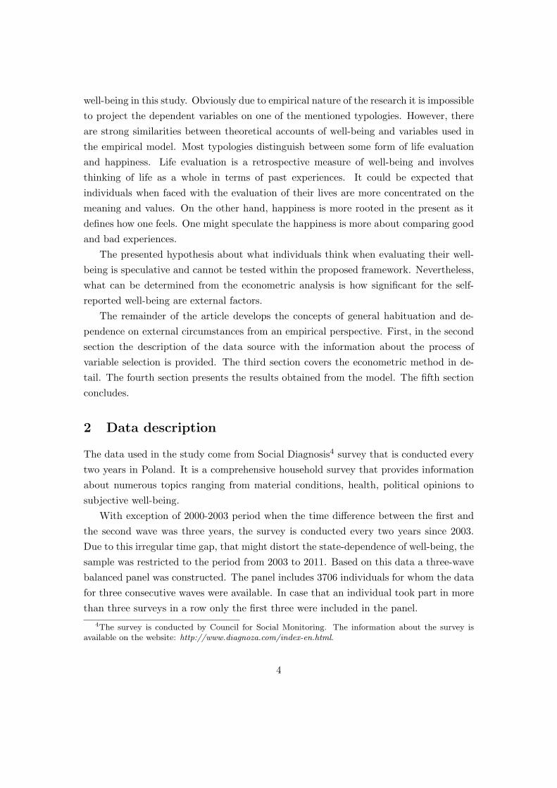
well-being in this study. Obviously due to empirical nature of the research it is impossible

to project the dependent variables on one of the mentioned typologies. However, there

are strong similarities between theoretical accounts of well-being and variables used in

the empirical model. Most typologies distinguish between some form of life evaluation

and happiness. Life evaluation is a retrospective measure of well-being and involves

thinking of life as a whole in terms of past experiences. It could be expected that

individuals when faced with the evaluation of their lives are more concentrated on the

meaning and values. On the other hand, happiness is more rooted in the present as it

defines how one feels. One might speculate the happiness is more about comparing good

and bad experiences.

The presented hypothesis about what individuals think when evaluating their well-

being is speculative and cannot be tested within the proposed framework. Nevertheless,

what can be determined from the econometric analysis is how significant for the self-

reported well-being are external factors.

The remainder of the article develops the concepts of general habituation and de-

pendence on external circumstances from an empirical perspective. First, in the second

section the description of the data source with the information about the process of

variable selection is provided. The third section covers the econometric method in de-

tail. The fourth section presents the results obtained from the model. The fifth section

concludes.

2 Data description

The data used in the study come from Social Diagnosis4 survey that is conducted every

two years in Poland. It is a comprehensive household survey that provides information

about numerous topics ranging from material conditions, health, political opinions to

subjective well-being.

With exception of 2000-2003 period when the time difference between the first and

the second wave was three years, the survey is conducted every two years since 2003.

Due to this irregular time gap, that might distort the state-dependence of well-being, the

sample was restricted to the period from 2003 to 2011. Based on this data a three-wave

balanced panel was constructed. The panel includes 3706 individuals for whom the data

for three consecutive waves were available. In case that an individual took part in more

than three surveys in a row only the first three were included in the panel.

4The survey is conducted by Council for Social Monitoring. The information about the survey isavailable on the website: http://www.diagnoza.com/index-en.html.

4

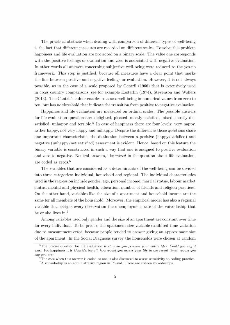
The practical obstacle when dealing with comparison of different types of well-being

is the fact that different measures are recorded on different scales. To solve this problem

happiness and life evaluation are projected on a binary scale. The value one corresponds

with the positive feelings or evaluation and zero is associated with negative evaluation.

In other words all answers concerning subjective well-being were reduced to the yes-no

framework. This step is justified, because all measures have a clear point that marks

the line between positive and negative feelings or evaluation. However, it is not always

possible, as in the case of a scale proposed by Cantril (1966) that is extensively used

in cross country comparisons, see for example Easterlin (1974), Stevenson and Wolfers

(2013). The Cantril’s ladder enables to assess well-being in numerical values from zero to

ten, but has no threshold that indicate the transition from positive to negative evaluation.

Happiness and life evaluation are measured on ordinal scales. The possible answers

for life evaluation question are: delighted, pleased, mostly satisfied, mixed, mostly dis-

satisfied, unhappy and terrible.5 In case of happiness there are four levels: very happy,

rather happy, not very happy and unhappy. Despite the differences those questions share

one important characteristic, the distinction between a positive (happy/satisfied) and

negative (unhappy/not satisfied) assessment is evident. Hence, based on this feature the

binary variable is constructed in such a way that one is assigned to positive evaluation

and zero to negative. Neutral answers, like mixed in the question about life evaluation,

are coded as zeros.6

The variables that are considered as a determinants of the well-being can be divided

into three categories: individual, household and regional. The individual characteristics

used in the regression include gender, age, personal income, martial status, labour market

status, mental and physical health, education, number of friends and religion practices.

On the other hand, variables like the size of a apartment and household income are the

same for all members of the household. Moreover, the empirical model has also a regional

variable that assigns every observation the unemployment rate of the voivodoship that

he or she lives in.7

Among variables used only gender and the size of an apartment are constant over time

for every individual. To be precise the apartment size variable exhibited time variation

due to measurement error, because people tended to answer giving an approximate size

of the apartment. In the Social Diagnosis survey the households were chosen at random

5The precise question for life evaluation is How do you perceive your entire life? Could you say itwas:. For happiness it is Considering all, how would you assess your life in the recent times would yousay you are:.

6The case when this answer is coded as one is also discussed to assess sensitivity to coding practice.7A voivodoship is an administrative region in Poland. There are sixteen voivodoships.

5

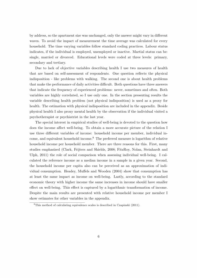
by address, so the apartment size was unchanged, only the answer might vary in different

waves. To avoid the impact of measurement the time average was calculated for every

household. The time varying variables follow standard coding practices. Labour status

indicates, if the individual is employed, unemployed or inactive. Martial status can be:

single, married or divorced. Educational levels were coded at three levels: primary,

secondary and tertiary.

Due to lack of objective variables describing health I use two measures of health

that are based on self-assessment of respondents. One question reflects the physical

indisposition - like problems with walking. The second one is about health problems

that make the performance of daily activities difficult. Both questions have three answers

that indicate the frequency of experienced problems: never, sometimes and often. Both

variables are highly correlated, so I use only one. In the section presenting results the

variable describing health problem (not physical indisposition) is used as a proxy for

health. The estimation with physical indisposition are included in the appendix. Beside

physical health I also proxy mental health by the observation if the individual visited a

psychotherapist or psychiatrist in the last year.

The special interest in empirical studies of well-being is devoted to the question how

does the income affect well-being. To obtain a more accurate picture of the relation I

use three different variables of income: household income per member, individual in-

come, and equivalent household income.8 The preferred measure is logarithm of relative

household income per household member. There are three reasons for this. First, many

studies emphasized (Clark, Frijters and Shields, 2008; FitzRoy, Nolan, Steinhardt and

Ulph, 2011) the role of social comparison when assessing individual well-being. I cal-

culated the reference income as a median income in a sample in a given year. Second,

the household income per capita also can be perceived as an approximation of indi-

vidual consumption. Headey, Muffels and Wooden (2004) show that consumption has

at least the same impact as income on well-being. Lastly, according to the standard

economic theory with higher income the same increases in income should have smaller

effect on well-being. This effect is captured by a logarithmic transformation of income.

Despite the main results are presented with relative household income per member I

show estimates for other variables in the appendix.

8This method of calculating equivalence scales is described in Czapinski (2011).

6

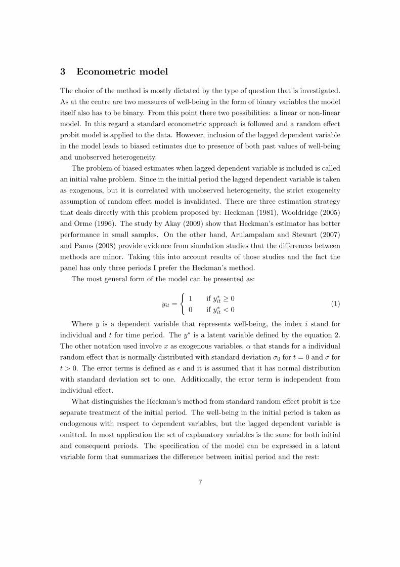
3 Econometric model

The choice of the method is mostly dictated by the type of question that is investigated.

As at the centre are two measures of well-being in the form of binary variables the model

itself also has to be binary. From this point there two possibilities: a linear or non-linear

model. In this regard a standard econometric approach is followed and a random effect

probit model is applied to the data. However, inclusion of the lagged dependent variable

in the model leads to biased estimates due to presence of both past values of well-being

and unobserved heterogeneity.

The problem of biased estimates when lagged dependent variable is included is called

an initial value problem. Since in the initial period the lagged dependent variable is taken

as exogenous, but it is correlated with unobserved heterogeneity, the strict exogeneity

assumption of random effect model is invalidated. There are three estimation strategy

that deals directly with this problem proposed by: Heckman (1981), Wooldridge (2005)

and Orme (1996). The study by Akay (2009) show that Heckman’s estimator has better

performance in small samples. On the other hand, Arulampalam and Stewart (2007)

and Panos (2008) provide evidence from simulation studies that the differences between

methods are minor. Taking this into account results of those studies and the fact the

panel has only three periods I prefer the Heckman’s method.

The most general form of the model can be presented as:

yit =

{

1 if y∗it≥ 0

0 if y∗it< 0

(1)

Where y is a dependent variable that represents well-being, the index i stand for

individual and t for time period. The y∗ is a latent variable defined by the equation 2.

The other notation used involve x as exogenous variables, α that stands for a individual

random effect that is normally distributed with standard deviation σ0 for t = 0 and σ for

t > 0. The error terms is defined as ǫ and it is assumed that it has normal distribution

with standard deviation set to one. Additionally, the error term is independent from

individual effect.

What distinguishes the Heckman’s method from standard random effect probit is the

separate treatment of the initial period. The well-being in the initial period is taken as

endogenous with respect to dependent variables, but the lagged dependent variable is

omitted. In most application the set of explanatory variables is the same for both initial

and consequent periods. The specification of the model can be expressed in a latent

variable form that summarizes the difference between initial period and the rest:

7

{

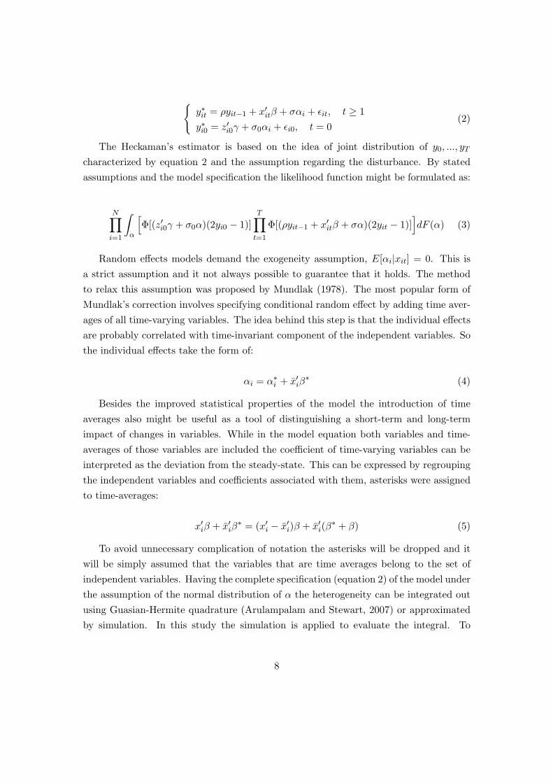
y∗it= ρyit−1 + x′

itβ + σαi + ǫit, t ≥ 1

y∗i0= z′

i0γ + σ0αi + ǫi0, t = 0

(2)

The Heckaman’s estimator is based on the idea of joint distribution of y0, ..., yT

characterized by equation 2 and the assumption regarding the disturbance. By stated

assumptions and the model specification the likelihood function might be formulated as:

N∏

i=1

∫

α

[

Φ[(z′i0γ + σ0α)(2yi0 − 1)]

T∏

t=1

Φ[(ρyit−1 + x′itβ + σα)(2yit − 1)]]

dF (α) (3)

Random effects models demand the exogeneity assumption, E[αi|xit] = 0. This is

a strict assumption and it not always possible to guarantee that it holds. The method

to relax this assumption was proposed by Mundlak (1978). The most popular form of

Mundlak’s correction involves specifying conditional random effect by adding time aver-

ages of all time-varying variables. The idea behind this step is that the individual effects

are probably correlated with time-invariant component of the independent variables. So

the individual effects take the form of:

αi = α∗i + x̄′iβ

∗ (4)

Besides the improved statistical properties of the model the introduction of time

averages also might be useful as a tool of distinguishing a short-term and long-term

impact of changes in variables. While in the model equation both variables and time-

averages of those variables are included the coefficient of time-varying variables can be

interpreted as the deviation from the steady-state. This can be expressed by regrouping

the independent variables and coefficients associated with them, asterisks were assigned

to time-averages:

x′iβ + x̄′iβ∗ = (x′i − x̄′i)β + x̄′i(β

∗ + β) (5)

To avoid unnecessary complication of notation the asterisks will be dropped and it

will be simply assumed that the variables that are time averages belong to the set of

independent variables. Having the complete specification (equation 2) of the model under

the assumption of the normal distribution of α the heterogeneity can be integrated out

using Guasian-Hermite quadrature (Arulampalam and Stewart, 2007) or approximated

by simulation. In this study the simulation is applied to evaluate the integral. To

8

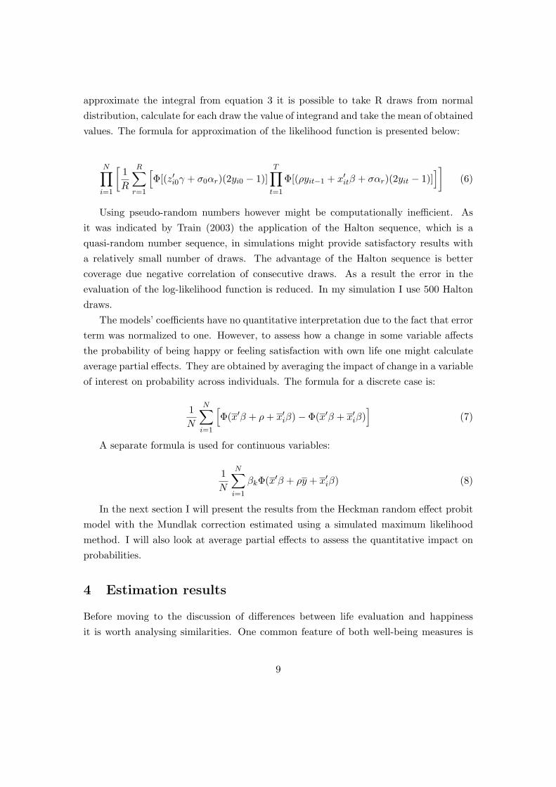
approximate the integral from equation 3 it is possible to take R draws from normal

distribution, calculate for each draw the value of integrand and take the mean of obtained

values. The formula for approximation of the likelihood function is presented below:

N∏

i=1

[

1

R

R∑

r=1

[

Φ[(z′i0γ + σ0αr)(2yi0 − 1)]T∏

t=1

Φ[(ρyit−1 + x′itβ + σαr)(2yit − 1)]]

]

(6)

Using pseudo-random numbers however might be computationally inefficient. As

it was indicated by Train (2003) the application of the Halton sequence, which is a

quasi-random number sequence, in simulations might provide satisfactory results with

a relatively small number of draws. The advantage of the Halton sequence is better

coverage due negative correlation of consecutive draws. As a result the error in the

evaluation of the log-likelihood function is reduced. In my simulation I use 500 Halton

draws.

The models’ coefficients have no quantitative interpretation due to the fact that error

term was normalized to one. However, to assess how a change in some variable affects

the probability of being happy or feeling satisfaction with own life one might calculate

average partial effects. They are obtained by averaging the impact of change in a variable

of interest on probability across individuals. The formula for a discrete case is:

1

N

N∑

i=1

[

Φ(x′β + ρ+ x′iβ)− Φ(x′β + x′iβ)]

(7)

A separate formula is used for continuous variables:

1

N

N∑

i=1

βkΦ(x′β + ρy + x′iβ) (8)

In the next section I will present the results from the Heckman random effect probit

model with the Mundlak correction estimated using a simulated maximum likelihood

method. I will also look at average partial effects to assess the quantitative impact on

probabilities.

4 Estimation results

Before moving to the discussion of differences between life evaluation and happiness

it is worth analysing similarities. One common feature of both well-being measures is

9

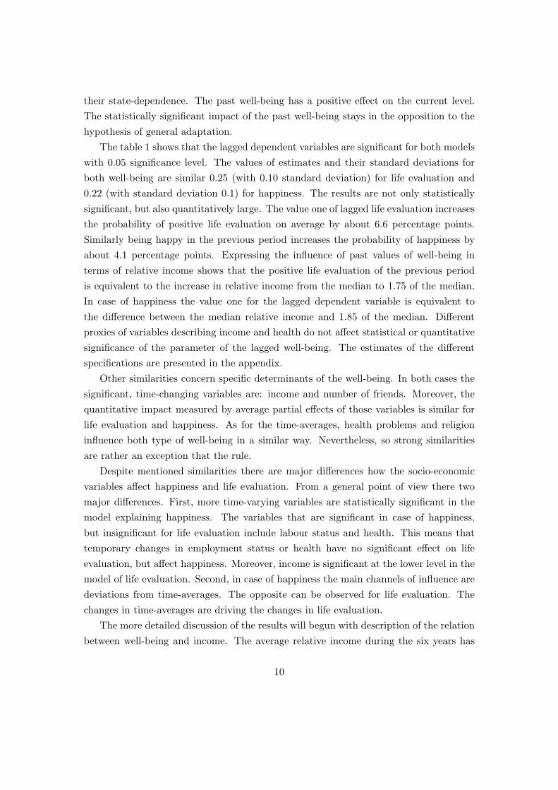
their state-dependence. The past well-being has a positive effect on the current level.

The statistically significant impact of the past well-being stays in the opposition to the

hypothesis of general adaptation.

The table 1 shows that the lagged dependent variables are significant for both models

with 0.05 significance level. The values of estimates and their standard deviations for

both well-being are similar 0.25 (with 0.10 standard deviation) for life evaluation and

0.22 (with standard deviation 0.1) for happiness. The results are not only statistically

significant, but also quantitatively large. The value one of lagged life evaluation increases

the probability of positive life evaluation on average by about 6.6 percentage points.

Similarly being happy in the previous period increases the probability of happiness by

about 4.1 percentage points. Expressing the influence of past values of well-being in

terms of relative income shows that the positive life evaluation of the previous period

is equivalent to the increase in relative income from the median to 1.75 of the median.

In case of happiness the value one for the lagged dependent variable is equivalent to

the difference between the median relative income and 1.85 of the median. Different

proxies of variables describing income and health do not affect statistical or quantitative

significance of the parameter of the lagged well-being. The estimates of the different

specifications are presented in the appendix.

Other similarities concern specific determinants of the well-being. In both cases the

significant, time-changing variables are: income and number of friends. Moreover, the

quantitative impact measured by average partial effects of those variables is similar for

life evaluation and happiness. As for the time-averages, health problems and religion

influence both type of well-being in a similar way. Nevertheless, so strong similarities

are rather an exception that the rule.

Despite mentioned similarities there are major differences how the socio-economic

variables affect happiness and life evaluation. From a general point of view there two

major differences. First, more time-varying variables are statistically significant in the

model explaining happiness. The variables that are significant in case of happiness,

but insignificant for life evaluation include labour status and health. This means that

temporary changes in employment status or health have no significant effect on life

evaluation, but affect happiness. Moreover, income is significant at the lower level in the

model of life evaluation. Second, in case of happiness the main channels of influence are

deviations from time-averages. The opposite can be observed for life evaluation. The

changes in time-averages are driving the changes in life evaluation.

The more detailed discussion of the results will begun with description of the relation

between well-being and income. The average relative income during the six years has

10

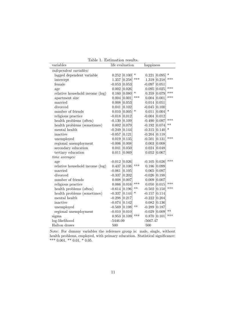
Table 1. Estimation results.variables life evaluation happiness

independent variables:lagged dependent variable 0.252 [0.100] * 0.221 [0.095] *intercept 1.357 [0.258] *** 1.319 [0.218] ***female -0.053 [0.053] -0.097 [0.051]age 0.002 [0.026] 0.095 [0.025] ***relative household income (log) 0.160 [0.080] * 0.359 [0.079] ***apartment size 0.004 [0.001] *** 0.004 [0.001] ***married 0.008 [0.053] 0.014 [0.051]divorced 0.041 [0.102] -0.045 [0.100]number of friends 0.010 [0.005] * 0.011 [0.004] *religious practice -0.018 [0.012] -0.004 [0.012]health problems (often) -0.130 [0.109] -0.490 [0.097] ***health problems (sometimes) 0.002 [0.079] -0.192 [0.074] **mental health -0.249 [0.144] -0.315 [0.140] *inactive -0.057 [0.121] -0.204 [0.118]unemployed 0.019 [0.135] -0.501 [0.131] ***regional unemployment -0.006 [0.008] 0.003 [0.008]secondary education 0.041 [0.050] 0.024 [0.048]tertiary education 0.011 [0.069] 0.052 [0.067]

time averages:age -0.012 [0.026] -0.105 [0.026] ***relative household income (log) 0.437 [0.106] *** 0.186 [0.099]married -0.061 [0.105] 0.065 [0.097]divorced -0.337 [0.202] -0.026 [0.198]number of friends 0.008 [0.007] 0.009 [0.007]religious practice 0.066 [0.016] *** 0.050 [0.015] ***health problems (often) -0.614 [0.196] ** -0.502 [0.150] ***health problems (sometimes) -0.337 [0.144] * -0.157 [0.114]mental health -0.298 [0.217] -0.222 [0.204]inactive -0.074 [0.142] 0.082 [0.136]unemployed -0.569 [0.198] ** -0.289 [0.187]regional unemployment -0.010 [0.010] -0.029 [0.009] **

sigma 0.953 [0.109] *** 0.870 [0.101] ***log-likelihood -5446.09 -5667.47Halton draws 500 500

Note: For dummy variables the reference group is: male, single, withouthealth problems, employed, with primary education. Statistical significance:*** 0.001, ** 0.01, * 0.05.

11

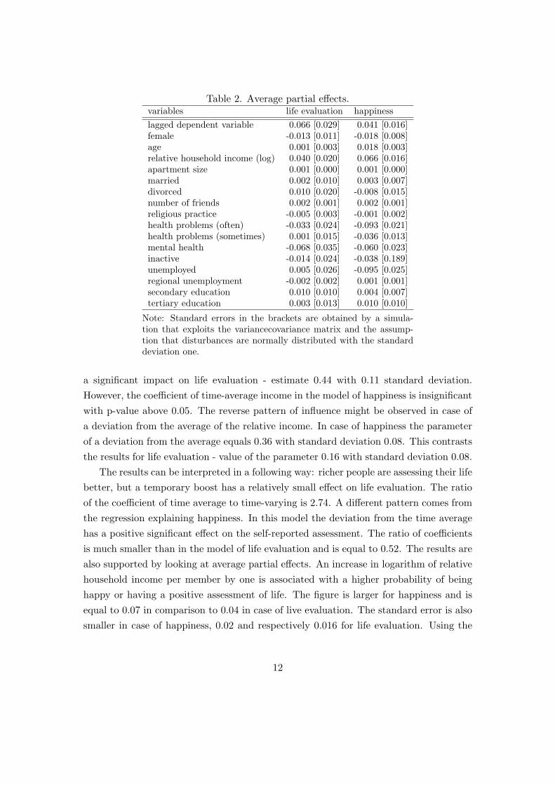
Table 2. Average partial effects.variables life evaluation happiness

lagged dependent variable 0.066 [0.029] 0.041 [0.016]female -0.013 [0.011] -0.018 [0.008]age 0.001 [0.003] 0.018 [0.003]relative household income (log) 0.040 [0.020] 0.066 [0.016]apartment size 0.001 [0.000] 0.001 [0.000]married 0.002 [0.010] 0.003 [0.007]divorced 0.010 [0.020] -0.008 [0.015]number of friends 0.002 [0.001] 0.002 [0.001]religious practice -0.005 [0.003] -0.001 [0.002]health problems (often) -0.033 [0.024] -0.093 [0.021]health problems (sometimes) 0.001 [0.015] -0.036 [0.013]mental health -0.068 [0.035] -0.060 [0.023]inactive -0.014 [0.024] -0.038 [0.189]unemployed 0.005 [0.026] -0.095 [0.025]regional unemployment -0.002 [0.002] 0.001 [0.001]secondary education 0.010 [0.010] 0.004 [0.007]tertiary education 0.003 [0.013] 0.010 [0.010]

Note: Standard errors in the brackets are obtained by a simula-tion that exploits the variancecovariance matrix and the assump-tion that disturbances are normally distributed with the standarddeviation one.

a significant impact on life evaluation - estimate 0.44 with 0.11 standard deviation.

However, the coefficient of time-average income in the model of happiness is insignificant

with p-value above 0.05. The reverse pattern of influence might be observed in case of

a deviation from the average of the relative income. In case of happiness the parameter

of a deviation from the average equals 0.36 with standard deviation 0.08. This contrasts

the results for life evaluation - value of the parameter 0.16 with standard deviation 0.08.

The results can be interpreted in a following way: richer people are assessing their life

better, but a temporary boost has a relatively small effect on life evaluation. The ratio

of the coefficient of time average to time-varying is 2.74. A different pattern comes from

the regression explaining happiness. In this model the deviation from the time average

has a positive significant effect on the self-reported assessment. The ratio of coefficients

is much smaller than in the model of life evaluation and is equal to 0.52. The results are

also supported by looking at average partial effects. An increase in logarithm of relative

household income per member by one is associated with a higher probability of being

happy or having a positive assessment of life. The figure is larger for happiness and is

equal to 0.07 in comparison to 0.04 in case of live evaluation. The standard error is also

smaller in case of happiness, 0.02 and respectively 0.016 for life evaluation. Using the

12

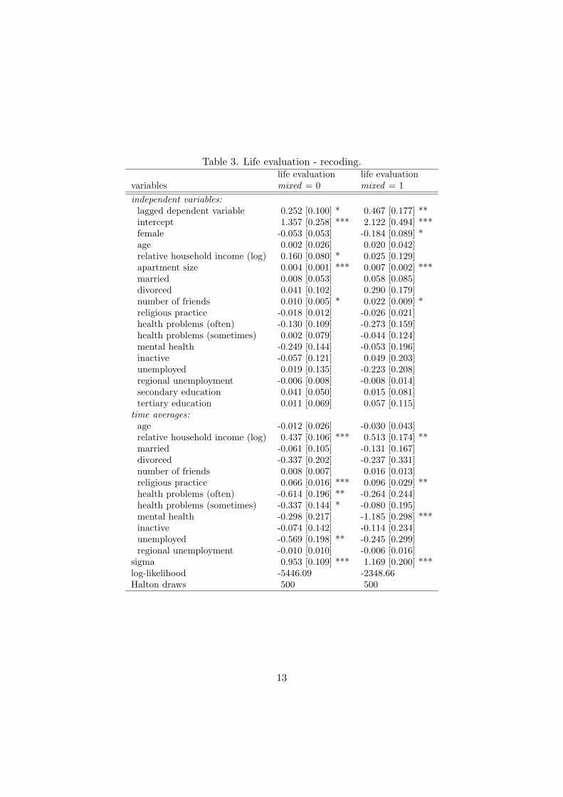
Table 3. Life evaluation - recoding.life evaluation life evaluation

variables mixed = 0 mixed = 1

independent variables:lagged dependent variable 0.252 [0.100] * 0.467 [0.177] **intercept 1.357 [0.258] *** 2.122 [0.494] ***female -0.053 [0.053] -0.184 [0.089] *age 0.002 [0.026] 0.020 [0.042]relative household income (log) 0.160 [0.080] * 0.025 [0.129]apartment size 0.004 [0.001] *** 0.007 [0.002] ***married 0.008 [0.053] 0.058 [0.085]divorced 0.041 [0.102] 0.290 [0.179]number of friends 0.010 [0.005] * 0.022 [0.009] *religious practice -0.018 [0.012] -0.026 [0.021]health problems (often) -0.130 [0.109] -0.273 [0.159]health problems (sometimes) 0.002 [0.079] -0.044 [0.124]mental health -0.249 [0.144] -0.053 [0.196]inactive -0.057 [0.121] 0.049 [0.203]unemployed 0.019 [0.135] -0.223 [0.208]regional unemployment -0.006 [0.008] -0.008 [0.014]secondary education 0.041 [0.050] 0.015 [0.081]tertiary education 0.011 [0.069] 0.057 [0.115]

time averages:age -0.012 [0.026] -0.030 [0.043]relative household income (log) 0.437 [0.106] *** 0.513 [0.174] **married -0.061 [0.105] -0.131 [0.167]divorced -0.337 [0.202] -0.237 [0.331]number of friends 0.008 [0.007] 0.016 [0.013]religious practice 0.066 [0.016] *** 0.096 [0.029] **health problems (often) -0.614 [0.196] ** -0.264 [0.244]health problems (sometimes) -0.337 [0.144] * -0.080 [0.195]mental health -0.298 [0.217] -1.185 [0.298] ***inactive -0.074 [0.142] -0.114 [0.234]unemployed -0.569 [0.198] ** -0.245 [0.299]regional unemployment -0.010 [0.010] -0.006 [0.016]

sigma 0.953 [0.109] *** 1.169 [0.200] ***log-likelihood -5446.09 -2348.66Halton draws 500 500

13

relative income without logarithmic transformation with additional squared value does

not affect results. Nevertheless, in general the logarithmic transformation yields better

fit that quadratic form.

The pattern showing that happiness is more dependant on current changes in income

is visible also for equivalent household income. The value of the parameter in the model

of happiness of the equivalent income change equals 0.36 with 0.08 standard deviation.

The numbers for life evaluation are -0.03 and 0.06 respectively. The impact of equivalent

income changes in case of life evaluation is even negative, but insignificant. The influence

of personal income on the well-being is negligible in both models.

The major difference between life evaluation and happiness in the context of health

is due to different strength of the impact of temporary changes in a health variable.

In case of happiness physical and mental health variables are significant and the effect

is quantitatively important. Having often health problem is associated with reduced

probability of being happy by 9 percentage points. The same figure for life evaluation is

3 percentage points. Mental problems translate into lower probability of happiness by 6

percentage points. This suggests that health is quantitatively significant contributor to

happiness. Additionally, none of the time varying health variables are significant in the

model of life evaluation. Replacing the health problems variable with disability variable

shows the same pattern of a strong impact of the deviations from the average in case of

happiness.

Changes in unemployment of a given individual are a significant determinant of

happiness. The value of the parameter of time-varying unemployment is 0.50 with a

standard deviation 0.13. The an average partial effect equals 0.10. This shows that

the state of unemployment increase the probability of being unhappy by 10 percentage

points. However, the same cannot be said of life evaluation. Moreover, for time average

there seems to be no relation between happiness and unemployment, but for life eval-

uation the estimates depends on how life evaluation was coded. The time-average of

regional unemployment has negative impact on well-being, but it is significant only in

case of happiness.

While the independent variable was constructed from ordinal scale there is possibility

that at least some results are driven by the coding method. To check this point I

recoded the life evaluation variable by setting 1 for the mixed answer. The table 3

shows that there is little difference between both models. The conclusions that might be

reached using the modified life evaluation are even sharper in comparison to the original

specification, while the new measure shows stronger state-dependence and is slightly less

dependant on external factors. The only difference is with the time average of mental

14

health variable. It is insignificant in the original model, but strongly significant with new

coding. For the new variable also long-term health is less important when determining

life evaluation. Nevertheless, the main results are consistent with both coding practices.

5 Conclusions

The study compares determinants and state-dependence of two different types of well-

being: life evaluation and happiness. The life evaluation represents a cognitive measure

and happiness is associated with an emotional assessment. The comparison indicates

that the evaluation of both types of well-being depend on their past values. The past

well-being has a statistically and quantitatively significant impact on the probability of a

positive assessment. The past positive life evaluation increases on average the probability

of having positive life evaluation by about 6 percentage points. In case of happiness the

corresponding figure is 4 percentage points.

Despite the common features both types of well-being differ in their determinants.

Life evaluation is less dependant on the external factors. The deviations from time

averages in case of income, labour status or health have relatively smaller influence on

life evaluation than on happiness. On the other hand, temporary changes in determinants

play a more important role in the model of happiness than of life evaluation.

15

Appendix

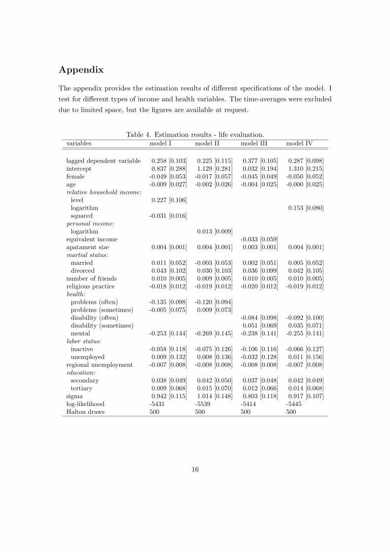
The appendix provides the estimation results of different specifications of the model. I

test for different types of income and health variables. The time-averages were excluded

due to limited space, but the figures are available at request.

Table 4. Estimation results - life evaluation.variables model I model II model III model IV

lagged dependent variable 0.258 [0.103] 0.225 [0.115] 0.377 [0.105] 0.287 [0.098]intercept 0.837 [0.288] 1.129 [0.281] 0.032 [0.194] 1.310 [0.215]female -0.049 [0.053] -0.017 [0.057] -0.045 [0.049] -0.050 [0.052]age -0.009 [0.027] -0.002 [0.026] -0.004 [0.025] -0.000 [0.025]relative household income:level 0.227 [0.106]logarithm 0.153 [0.080]squared -0.031 [0.016]

personal income:logarithm 0.013 [0.009]

equivalent income -0.033 [0.059]apatament size 0.004 [0.001] 0.004 [0.001] 0.003 [0.001] 0.004 [0.001]martial status:married 0.011 [0.052] -0.003 [0.053] 0.002 [0.051] 0.005 [0.052]divorced 0.043 [0.102] 0.030 [0.103] 0.036 [0.099] 0.042 [0.105]

number of friends 0.010 [0.005] 0.009 [0.005] 0.010 [0.005] 0.010 [0.005]religious practice -0.018 [0.012] -0.019 [0.012] -0.020 [0.012] -0.019 [0.012]health:problems (often) -0.135 [0.098] -0.120 [0.094]problems (sometimes) -0.005 [0.075] 0.009 [0.073]disability (often) -0.084 [0.098] -0.092 [0.100]disability (sometimes) 0.051 [0.069] 0.035 [0.071]mental -0.253 [0.144] -0.269 [0.145] -0.238 [0.141] -0.255 [0.141]

labor status:inactive -0.058 [0.118] -0.075 [0.126] -0.106 [0.116] -0.066 [0.127]unemployed 0.009 [0.132] 0.008 [0.136] -0.032 [0.128] 0.011 [0.156]

regional unemployment -0.007 [0.008] -0.008 [0.008] -0.008 [0.008] -0.007 [0.008]education:secondary 0.038 [0.049] 0.042 [0.050] 0.037 [0.048] 0.042 [0.049]tertiary 0.009 [0.068] 0.015 [0.070] 0.012 [0.066] 0.014 [0.068]

sigma 0.942 [0.115] 1.014 [0.148] 0.803 [0.118] 0.917 [0.107]log-likelihood -5431 -5539 -5414 -5445Halton draws 500 500 500 500

16

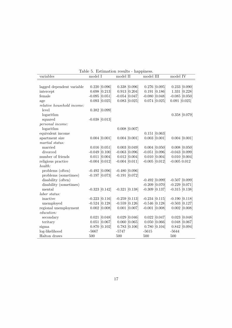
Table 5. Estimation results - happiness.variables model I model II model III model IV

lagged dependent variable 0.220 [0.096] 0.338 [0.096] 0.276 [0.095] 0.233 [0.090]intercept 0.698 [0.213] 0.913 [0.204] 0.191 [0.186] 1.331 [0.228]female -0.095 [0.051] -0.054 [0.047] -0.080 [0.048] -0.085 [0.050]age 0.093 [0.025] 0.083 [0.025] 0.074 [0.025] 0.091 [0.025]relative household income:level 0.382 [0.099]logarithm 0.358 [0.079]squared -0.038 [0.013]

personal income:logarithm 0.008 [0.007]

equivalent income 0.151 [0.063]apartment size 0.004 [0.001] 0.004 [0.001] 0.003 [0.001] 0.004 [0.001]martial status:married 0.016 [0.051] 0.003 [0.049] 0.004 [0.050] 0.008 [0.050]divorced -0.049 [0.100] -0.063 [0.096] -0.051 [0.096] -0.043 [0.099]

number of friends 0.011 [0.004] 0.012 [0.004] 0.010 [0.004] 0.010 [0.004]religious practice -0.004 [0.012] -0.004 [0.011] -0.005 [0.012] -0.005 0.012health:problems (often) -0.492 [0.096] -0.480 [0.096]problems (sometimes) -0.197 [0.073] -0.191 [0.072]disability (often) -0.492 [0.099] -0.507 [0.099]disability (sometimes) -0.209 [0.070] -0.229 [0.071]mental -0.323 [0.142] -0.321 [0.138] -0.309 [0.137] -0.315 [0.138]

labor status:inactive -0.223 [0.116] -0.259 [0.113] -0.234 [0.115] -0.190 [0.118]unemployed -0.524 [0.128] -0.559 [0.126] -0.546 [0.128] -0.503 [0.127]

regional unemployment 0.002 [0.008] 0.001 [0.007] -0.001 [0.008] 0.002 [0.008]education:secondary 0.021 [0.048] 0.029 [0.046] 0.022 [0.047] 0.023 [0.048]teritary 0.051 [0.067] 0.060 [0.065] 0.050 [0.066] 0.048 [0.067]

sigma 0.870 [0.102] 0.783 [0.106] 0.780 [0.104] 0.842 [0.094]log-likelihood -5667 -5747 -5615 -5644Halton draws 500 500 500 500

17

References

Akay, A. (2009), The wooldridge method for the initial values problem is simple: What

about performance?, IZA Discussion Papers 3943, Institute for the Study of Labor

(IZA).

Arulampalam, W. and Stewart, M. (2007), Simplified implementation of the heckman

estimator of the dynamic probit model and a comparison with alternative estimators,

IZA Discussion Papers 3039, Institute for the Study of Labor (IZA).

Binder, M. and Coad, A. (2010), ‘An examination of the dynamics of well-being and life

events using vector autoregressions’, Journal of Economic Behavior & Organization

76(2), 352–371.

Bottan, N. L. and Perez Truglia, R. (2011), ‘Deconstructing the hedonic treadmill: Is

happiness autoregressive?’, The Journal of Socio-Economics 40(3), 224–236.

Cantril, H. (1966), The pattern of human concerns, ICPSR study, Rutgers University

Press.

Clark, A. E. (2006), ‘A note on unhappiness and unemployment duration’, Applied

Economics Quarterly (formerly: Konjunkturpolitik) 52(4), 291–308.

Clark, A. E., Diener, E., Georgellis, Y. and Lucas, R. E. (2004), ‘Unemployment alters

the set point for life satisfaction.’, Psychol Sci 15(1), 8–13.

Clark, A. E., Diener, E., Georgellis, Y. and Lucas, R. E. (2008), ‘Lags and leads in life

satisfaction: a test of the baseline hypothesis’, Economic Journal 118(529), F222–

F243.

Clark, A. E., Frijters, P. and Shields, M. A. (2008), ‘Relative income, happiness, and util-

ity: An explanation for the easterlin paradox and other puzzles’, Journal of Economic

Literature 46(1), 95–144.

Council for Social Monitoring (n.d.), ‘Social diagnosis 2000-2011: integrated database’.

Czapinski, J. (1991), ‘Illusions and biases in psychological well-being: An ’onion’theory

of happiness.’, Paper presented at the Working Meeting of I.S.R. and I.S.S., 1991,

University of Michigan, Ann Arbor, USA .

Czapinski, J. (2011), ‘Social diagnosis 2011 objective and subjective quality of life in

poland - full report’, Contemporary Economics 5(3).

18

Di Tella, R., Haisken-De New, J. and MacCulloch, R. (2010), ‘Happiness adaptation

to income and to status in an individual panel’, Journal of Economic Behavior &

Organization 76(3), 834–852.

Dolan, P., Peasgood, T. and White, M. (2006), Review of research on the influence of

personal well-being and application to policy making., Report for defra.

Easterlin, R. A. (1974), ‘Does economic growth improve the human lot? Some empirical

evidence’, Nations and households in economic growth 89.

FitzRoy, F. R., Nolan, M. A., Steinhardt, M. F. and Ulph, D. (2011), ‘So far so good:

Age, happiness, and relative income’, (415).

Gardner, J. and Oswald, A. J. (2006), ‘Do divorcing couples become happier by breaking

up?’, Journal of the Royal Statistical Society Series A 169(2), 319–336.

Headey, B., Muffels, R. and Wooden, M. (2004), Money doesnt buy happiness or does it?

a reconsideration based on the combined effects of wealth, income and consumption,

IZA Discussion Papers 1218, Institute for the Study of Labor (IZA).

Headey, B. and Wearing, A. (1989), ‘Personality, life events, and subjective well-being:

Toward a dynamic equilibrium model’, Journal of Personality and Social Psychology

57, 731–739.

Heckman, J. J. (1981), Heterogeneity and state dependence, in ‘Studies in Labor Mar-

kets’, NBER Chapters, National Bureau of Economic Research, Inc, pp. 91–140.

Kahneman, D. (1999), ‘Experienced utility and objective happiness: A moment-based

approach’, The Psychology of Economic Decisions: Rationality and well-being .

Kahneman, D. and Deaton, A. (2010), ‘High income improves evaluation of life

but not emotional well-being’, Proceedings of the National Academy of Sciences

107(38), 16489–16493.

Lee, W.-S. and Oguzoglu, U. (2007), Are youths on income support less happy? evidence

from australia, Iza discussion papers, Institute for the Study of Labor (IZA).

Mundlak, Y. (1978), ‘On the pooling of time series and cross section data’, Econometrica

46(1), 69–85.

Orme, C. (1996), The Initial Conditions Problem and Two-step Estimation in Discrete

Panel Data Models, Discussion paper series, University of Manchester.

19

Panos, S. (2008), State dependence in work-related training participation among british

employees: A comparison of different random effects probit estimators, MPRA Paper

14261, University Library of Munich, Germany.

Piper, A. T. (2012), Dynamic analysis and the economics of happiness: Rationale, results

and rules, MPRA Paper 43248, University Library of Munich, Germany.

Pudney, S. (2008), ‘The dynamics of perception: modelling subjective wellbeing in a

short panel’, Journal of the Royal Statistical Society Series A 171(1), 21–40.

Seligman, M. (2011), Authentic Happiness, Random House Australia.

Stevenson, B. and Wolfers, J. (2013), ‘Subjective well-being and income: Is there any

evidence of satiation?’, American Economic Review 103(3), 598–604.

Train, K. (2003), Discrete Choice Methods With Simulation, Discrete Choice Methods

with Simulation, Cambridge University Press.

Wong, P. T. (2011), ‘Positive psychology 2.0: Towards a balanced interactive model of

the good life.’, Canadian Psychology 52(2)(2).

Wooldridge, J. M. (2005), ‘Simple solutions to the initial conditions problem in dy-

namic, nonlinear panel data models with unobserved heterogeneity’, Journal of Ap-

plied Econometrics 20(1), 39–54.

Zimmermann, A. C. and Easterlin, R. A. (2006), ‘Happily ever after? cohabitation,

marriage, divorce, and happiness in germany’, Population and Development Review

32(3), 511–528.

20