download (788kb) - munich personal repec archive
TRANSCRIPT
Munich Personal RePEc Archive
Insight of Indian sector indices for the
post subprime crisis period: a vector
error correction model approach
Vardhan, Harsh and Vij, Madhu and Sinha, Pankaj
Faculty of Management Studies, University of Delhi
September 2013
Online at https://mpra.ub.uni-muenchen.de/49962/
MPRA Paper No. 49962, posted 19 Sep 2013 12:33 UTC
1
Insight of Indian sector indices for the post subprime crisis period: a
vector error correction model approach
Harsh Vardhan, Madhu Vij and Pankaj Sinha
Faculty of Management Studies, University of Delhi
Abstract
The empirical study highlights importance of usage of sector indices which provides insight for sector
specific investment strategies and direction for suitable policy formulation. It investigates long run and
short run relationships between eight identified sector indices and Sensex for the post subprime period
from 04/09/2009 to 31/12/2010 using Vector Error Correction Model (VECM). Limited lead - lag short
run relationships between sector indices were observed. Long term relationships between sector indices
were determined by the usage of VECM indicating minimal benefits from diversifying investments to
different sectors. Banking index played a predominant and integrating role in moving other indices.
During this period of recovery; most sectors were protected and provided marginally better returns due
to robust Banking policy. Realty & Metal were other significant drivers influencing remaining sectors
contemporaneously.
Key words: Vector Error Correction Model (VECM), Sector Index, Generalized Impulse
Response Function (GIRF).
JEL Classification B22 E60 C22 G18 C01
2
1. Introduction
The US sub-prime mortgage crisis created financial chaos engulfing the global economy during
2007-09. The crisis manifested how external shock traverses the interlinked global economies
perishing demand of exports and enhancing reversal of capital inflows. Its direct consequence
was reflected in the crash of the global stock market, credit crunch, and decline in the growth of
production. In 2009, the world trade contracted by 12.5% in volume terms, Asia’s exports
declined by 11.5% and imports by around 7.9% (WTO, 2010). The emerging Asian economies
registered growth of 5.7%, whereas, others registered negative growth in real GDP, US (–2.4%),
World (–0.6%) and Euro zone (–4.1%) (IMF 2010; Das 2011). Asian economies including India
were also affected due to global meltdown. The GDP contraction in Asia was 15% on seasonally
adjusted annualized basis for the fourth quarter of 2008,1 but they firmly led the global recovery.
The Asian economies’ role during recessionary period was recognized2. The three economies,
China, Indonesia and India were the only exception of not showing negative GDP growth and
remained resilient in the face of the intense global crisis and recession (Das DK, 2010, 2011).
The study uses sectoral indices and the Sensex for transmission of information and
understanding its pattern across various sectors which may have utility for institutional investors
for emerging markets. A few studies were done using sector indices as a benchmark to track
performance of actively managed portfolios (Ewing 2002; Ewing et al. 2003; Wang et al.
2005). Some research conducted using multivariate cointegration analysis by VECM for
studying transmission of information are by Fayoumi et al.(2009) for sector index of Amman
Stock Exchange (ASE), Poshakwale S & Patra T(2008) for long-run and short-run relationship
between major stock indices of the Athens Stock Exchange (ASE),Wang & Yang (2005) for
major sector indices of Chinese stock exchange, Ewing BT(2002) for five S&P stock indices and
Arbelaez H et al. (2001) for interlinkages of the Colombian stock exchange. These studies have
highlighted utility and importance of usage of sector indices; some exhibited long-run
relationship as well as short-run relationship, and also exhibited transmission of innovation to
1 IMF (2009), Regional Economic Outlook: Asia & Pacific Washington DC May.
2According to D Strauss-Kahn, former MD International Monetary Fund, “Asia has shown remarkable resilience
during the global financial crisis and emerged as an economic powerhouse that is leading the global recovery. There
are important lessons for other regions. In particular, the extensive reforms undertaken over the past decade have
been critical in helping to protect Asia from the full brunt of the crisis.”IMF Press release 10/290.
3
interlinked sectors in different proportions in a short span. As no study using VAR has been
employed for the post subprime crisis period using sector indices for the Indian economy, this
study will be helpful for sector focus investment strategy and policy formulation.
The study will confirm resilience of the Indian economy by understanding the importance and
behavior of interrelated sector indices and Sensex in the dynamic economic environment. It also
attempts to answer the question: Do the different sector indices get influenced to move together
in a similar way in the long-run? Is there a lead lag relationship between the sectoral indices for
the short-run? Which are the growth driving and integrating sector index? What are the sector
specific policy implications for sustained growth?
2. Data & Methodology
The sample data for the study are the closing price for 11 sector indices - SENSEX, BANKEX,
IT, OIL & GAS, FMCG, AUTO, CG, METAL, CD, HCARE, INFRA and POWER. The data
comprising of 450 observations has been obtained from BSE and CMIE databases and it has
been transformed into logarithmic scale. The sample period for the post subprime crisis
timeframe is from 10th
March 2009 to 31st December 2010.The daily return R(Index)t, i is
calculated by the following:
R(Index)t, i = [log ( )]*100, where P(Index)t, i is the closing price for ith sector on t
th day.
The stationarity of time series of indices is checked by ADF, PP & KPSS tests. The Akaike’s
Information Criterion (AIC) and Schwarz Bayesian Criterion (SBC) are used for selection of
suitable lag length. The cointegration is tested for VAR model using Johansen & Juselius (1990)
technique employing trace and maximum Eigen value statistics. In case cointegration exits;
Vector Error Correction Model (VECM) is appropriate for further econometric analysis and for
examining causality relationships. The Granger causality/Block Exogeneity Wald test is
employed to assess whether inclusion of the lagged value of a variable is important in explaining
dynamics of other variables in the multivariate frame work in addition to the explanatory power
of lag of these variables [Ahmed A.E (2011)]. If no cointegration exists between the indices,
short run relationships between the sector indices are examined by employing Granger
Causality test (1969, 1988) for the VAR model.
4
The study uses generalized impulse response function (GIFR) that is insensitive to the ordering
of the variables in the VAR model. It also provides more robust results than the orthogonalized
method. Generalized Impulse Response and Variance decomposition analysis provides
information about precise interplay of sector indices. Impulse Response Function (IRF)
manifests effect of a random shock (unpredicted) which happens through one of the innovations
on the current and future index prices. The IRF quantifies duration of the effect of innovations in
one sectoral index to itself and other indices.
The variance decomposition which is an out-of sample causality test (Arbelaez et al. 2001)
shows that the proportion of movements in the dependent variables that are due to their own
shock versus shock to the other variables. It partitions the variance of the forecast error of a
variable into proportions relating to shock in each sector index including its own. It is evident
that a variable that optimally forecasts using its own lagged values will have all its forecast
variance accounted for its own disturbance (Sim, 1982).
Vector Error Correction Model
The Vector Error Correction Model for Yt=A1Yt-1 + C1+ut is given by
∆Yt=Γ1∆Yt-1 +ПYt-1+C+ut , where Yt is a matrix of endogenous variables, Γ1∆Yt-1 relates to
short term relationship and П8x8Yt-1 is error correction term for long run relationship. The impact
matrix П contains information pertaining to long run relationship between the sector indices and
the rank of П indicates number of co integrating relationships.
Πgxg =αβ', where αg*r and β'r*g
g=number of variables
r=rank or number of co integrating vectors, , here g=8, r=2 and k=1
α is speed of adjustment to equilibrium coefficient or amount of co integrating vector entering in each
equation of VECM or adjustment coefficient or loading in each regression.
β' long run matrix of coefficients or co integrating vector
β'yt-1 = error correction term,
5
yt is matrix of variables which are endogenous;
βij ;i=(1,2….8) number of variables and j= 1,2 ; number of co integrating equations
α8*2 = β8*2 = П8*8=
3. Data Analysis for post recessionary period [4/09/2009 to 31/12/2010]
Descriptive Statistics
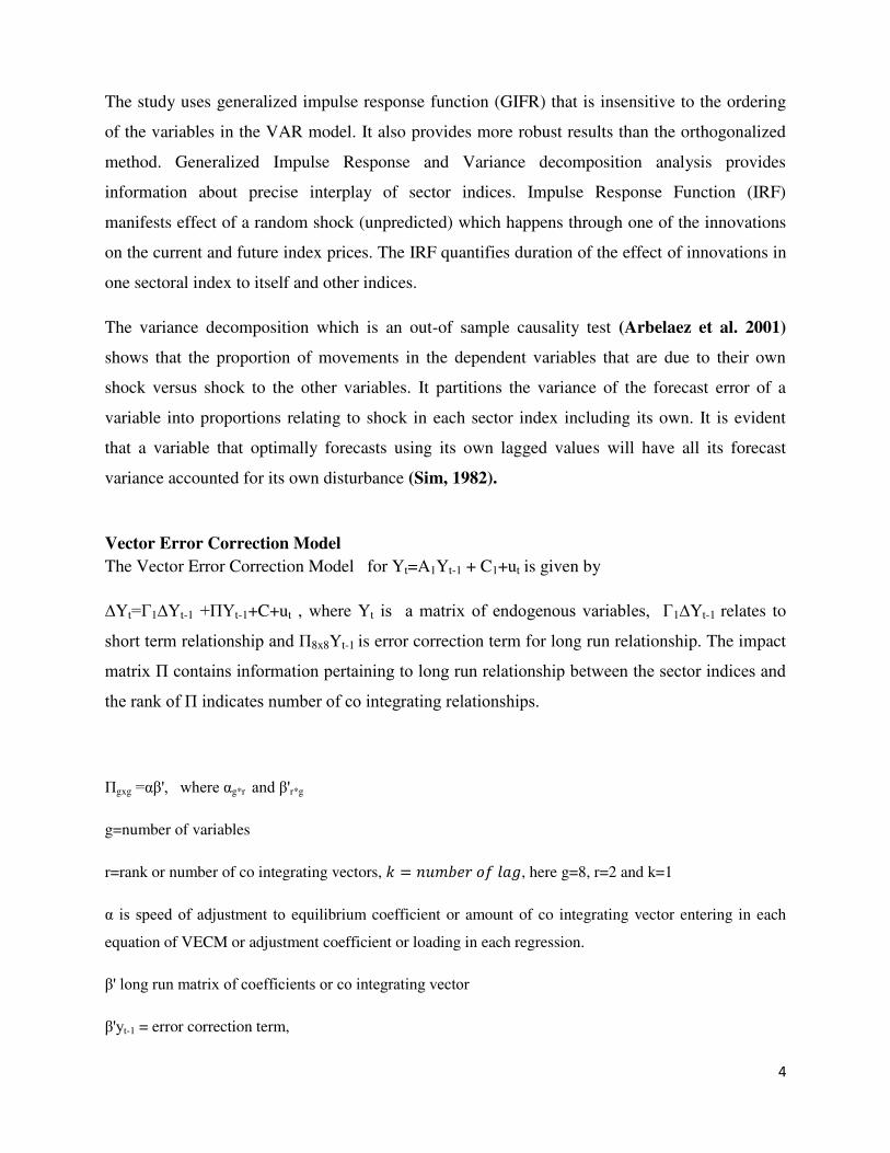
The line plots of log of sectoral indices and Sensex for the period of recovery [10/03/2009 to
31/12/2010] shows an upward trend for all log series. This gradually stabilizes, tracing an almost
uniform pattern indicating that market information influences in a similar fashion (Figure 1).
Figure 1: Line diagram of Log of indices
Source: Compiled from CMIE data base
7.0
7.5
8.0
8.5
9.0
9.5
10.0
50 100 150 200 250 300 350 400 450
LSENSEX LBANKEX LITLOILGAS LFMCG LAUTOLCG LMETAL LCDLPOWER LREALTY LHCARE

6
All log transformed indices are negatively skewed. The JB statistics for normality of residual
shows that these series are not normally distributed. The coefficient of variation analysis shows
that the Consumer Durables is highly volatile and it is followed by IT, Bankex and Health care.
The descriptive statistics of returns of indices shows that the highest return is for Consumer
Durable followed by Metal, Auto and Bankex. Power registered lowest returns. These returns are
positively skewed and their distributions are leptokurtic. The coefficient of variation which is
also a measure of riskiness indicates highest volatility of returns for Oil & Gas; followed by for
Capital Goods, FMCG and Bankex. A low relative volatility is observed for Health care and
Auto sector.
The contemporaneous correlation matrix for index return indicates that Sensex returns are highly
positively correlated with the returns of Bankex (0.9052), Power (0.9014), Capital Goods
(0.8783) and Oil & Gas (0.86760). It is also observed that Bankex index moves with Capital
Goods and Power index indicating strong relationship with these two indices. Power is highly
positively correlated with Capital Goods (0.9063), Metal (0.8160) and Realty index (0.8188)
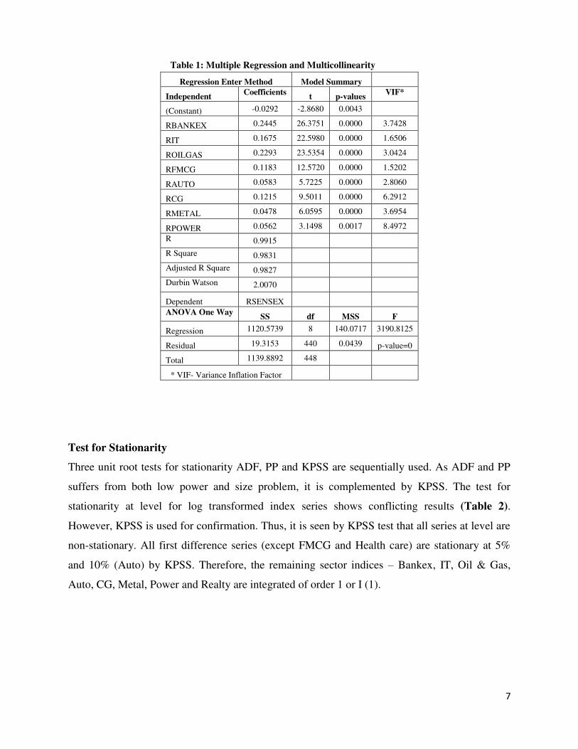
The multiple regression analysis of Sensex return on 10 sectoral indices indicates Adj R2 is very
high 0.983. The goodness of fit is confirmed by the one way ANOVA as p-value = 0.00. The
Variance Inflation Factors (VIFs) for all index return are less than 10 indicating that no
multicollinearity exists. The value of t-statistics for Realty and Healthcare are negative and
insignificant at 5% level of significance. Therefore, Realty and Health care indices are removed
from the model. The improved multiple regression model consists of regression of Sensex on
remaining 8 indices. The Adj R2
remains high (0.983). It is also seen that t-values are significant
and are positive. Thus it is a better robust and reliable model (Table 1)
7
Table 1: Multiple Regression and Multicollinearity
Regression Enter Method Model Summary
Independent Coefficients
t p-values VIF*
(Constant) -0.0292 -2.8680 0.0043
RBANKEX 0.2445 26.3751 0.0000 3.7428
RIT 0.1675 22.5980 0.0000 1.6506
ROILGAS 0.2293 23.5354 0.0000 3.0424
RFMCG 0.1183 12.5720 0.0000 1.5202
RAUTO 0.0583 5.7225 0.0000 2.8060
RCG 0.1215 9.5011 0.0000 6.2912
RMETAL 0.0478 6.0595 0.0000 3.6954
RPOWER 0.0562 3.1498 0.0017 8.4972
R 0.9915
R Square 0.9831
Adjusted R Square 0.9827
Durbin Watson 2.0070
Dependent RSENSEX
ANOVA One Way SS df MSS F
Regression 1120.5739 8 140.0717 3190.8125
Residual 19.3153 440 0.0439 p-value=0
Total 1139.8892 448
* VIF- Variance Inflation Factor
Test for Stationarity
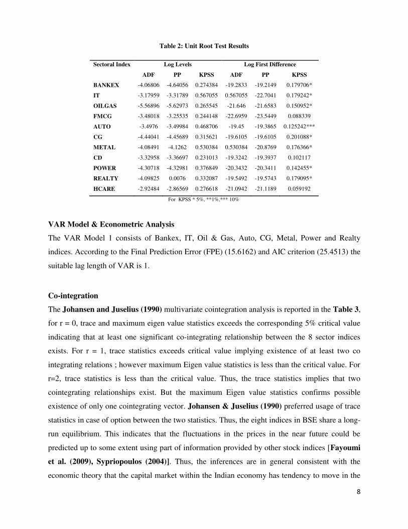
Three unit root tests for stationarity ADF, PP and KPSS are sequentially used. As ADF and PP
suffers from both low power and size problem, it is complemented by KPSS. The test for
stationarity at level for log transformed index series shows conflicting results (Table 2).
However, KPSS is used for confirmation. Thus, it is seen by KPSS test that all series at level are
non-stationary. All first difference series (except FMCG and Health care) are stationary at 5%
and 10% (Auto) by KPSS. Therefore, the remaining sector indices – Bankex, IT, Oil & Gas,
Auto, CG, Metal, Power and Realty are integrated of order 1 or I (1).
8
Table 2: Unit Root Test Results
Sectoral Index Log Levels Log First Difference
ADF PP KPSS ADF PP KPSS
BANKEX -4.06806 -4.64056 0.274384 -19.2833 -19.2149 0.179706*
IT -3.17959 -3.31789 0.567055 0.567055 -22.7041 0.179242*
OILGAS -5.56896 -5.62973 0.265545 -21.646 -21.6583 0.150952*
FMCG -3.48018 -3.25535 0.244148 -22.6959 -23.5449 0.088339
AUTO -3.4976 -3.49984 0.468706 -19.45 -19.3865 0.125242***
CG -4.44041 -4.45689 0.315621 -19.6105 -19.6105 0.201088*
METAL -4.08491 -4.1262 0.530384 0.530384 -20.8769 0.176366*
CD -3.32958 -3.36697 0.231013 -19.3242 -19.3937 0.102117
POWER -4.30718 -4.32981 0.376849 -20.3432 -20.3411 0.142455*
REALTY -4.09825 0.0076 0.332087 -19.5492 -19.5743 0.179095*
HCARE -2.92484 -2.86569 0.276618 -21.0942 -21.1189 0.059192
For KPSS * 5%, **1%,*** 10%
VAR Model & Econometric Analysis
The VAR Model 1 consists of Bankex, IT, Oil & Gas, Auto, CG, Metal, Power and Realty
indices. According to the Final Prediction Error (FPE) (15.6162) and AIC criterion (25.4513) the
suitable lag length of VAR is 1.
Co-integration
The Johansen and Juselius (1990) multivariate cointegration analysis is reported in the Table 3,
for r = 0, trace and maximum eigen value statistics exceeds the corresponding 5% critical value
indicating that at least one significant co-integrating relationship between the 8 sector indices
exists. For r = 1, trace statistics exceeds critical value implying existence of at least two co
integrating relations ; however maximum Eigen value statistics is less than the critical value. For
r=2, trace statistics is less than the critical value. Thus, the trace statistics implies that two
cointegrating relationships exist. But the maximum Eigen value statistics confirms possible
existence of only one cointegrating vector. Johansen & Juselius (1990) preferred usage of trace
statistics in case of option between the two statistics. Thus, the eight indices in BSE share a long-
run equilibrium. This indicates that the fluctuations in the prices in the near future could be
predicted up to some extent using part of information provided by other stock indices [Fayoumi
et al. (2009), Sypriopoulos (2004)]. Thus, the inferences are in general consistent with the
economic theory that the capital market within the Indian economy has tendency to move in the
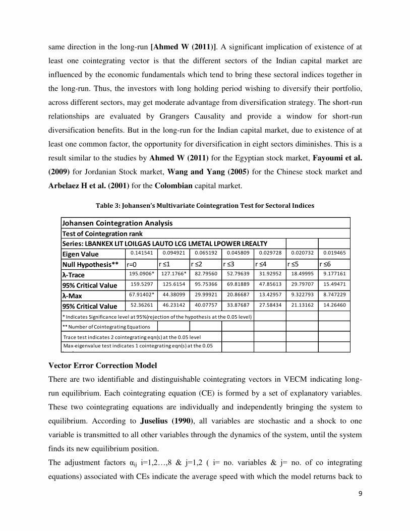
9
same direction in the long-run [Ahmed W (2011)]. A significant implication of existence of at
least one cointegrating vector is that the different sectors of the Indian capital market are
influenced by the economic fundamentals which tend to bring these sectoral indices together in
the long-run. Thus, the investors with long holding period wishing to diversify their portfolio,
across different sectors, may get moderate advantage from diversification strategy. The short-run
relationships are evaluated by Grangers Causality and provide a window for short-run
diversification benefits. But in the long-run for the Indian capital market, due to existence of at
least one common factor, the opportunity for diversification in eight sectors diminishes. This is a
result similar to the studies by Ahmed W (2011) for the Egyptian stock market, Fayoumi et al.
(2009) for Jordanian Stock market, Wang and Yang (2005) for the Chinese stock market and
Arbelaez H et al. (2001) for the Colombian capital market.
Table 3: Johansen’s Multivariate Cointegration Test for Sectoral Indices
Vector Error Correction Model
There are two identifiable and distinguishable cointegrating vectors in VECM indicating long-
run equilibrium. Each cointegrating equation (CE) is formed by a set of explanatory variables.
These two cointegrating equations are individually and independently bringing the system to
equilibrium. According to Juselius (1990), all variables are stochastic and a shock to one
variable is transmitted to all other variables through the dynamics of the system, until the system
finds its new equilibrium position.
The adjustment factors αij i=1,2…,8 & j=1,2 ( i= no. variables & j= no. of co integrating
equations) associated with CEs indicate the average speed with which the model returns back to
0.141541 0.094921 0.065192 0.045809 0.029728 0.020732 0.019465
r=0 r ≤1 r ≤2 r ≤3 r ≤4 r ≤5 r ≤6 195.0906* 127.1766* 82.79560 52.79639 31.92952 18.49995 9.177161
159.5297 125.6154 95.75366 69.81889 47.85613 29.79707 15.49471
67.91402* 44.38099 29.99921 20.86687 13.42957 9.322793 8.747229
52.36261 46.23142 40.07757 33.87687 27.58434 21.13162 14.26460
* Indicates Significance level at 95%(rejection of the hypothesis at the 0.05 level)
Series: LBANKEX LIT LOILGAS LAUTO LCG LMETAL LPOWER LREALTY
Test of Cointegration rank
Johansen Cointegration Analysis
Max-eigenvalue test indicates 1 cointegrating eqn(s) at the 0.05
level
Trace test indicates 2 cointegrating eqn(s) at the 0.05 level
Eigen Value
Null Hypothesis**
95% Critical Value
95% Critical Value
** Number of Cointegrating Equations
λ-Trace
λ-Max
10
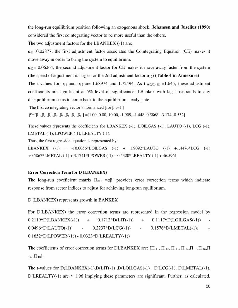
the long-run equilibrium position following an exogenous shock. Johansen and Juselius (1990)
considered the first cointegrating vector to be more useful than the others.
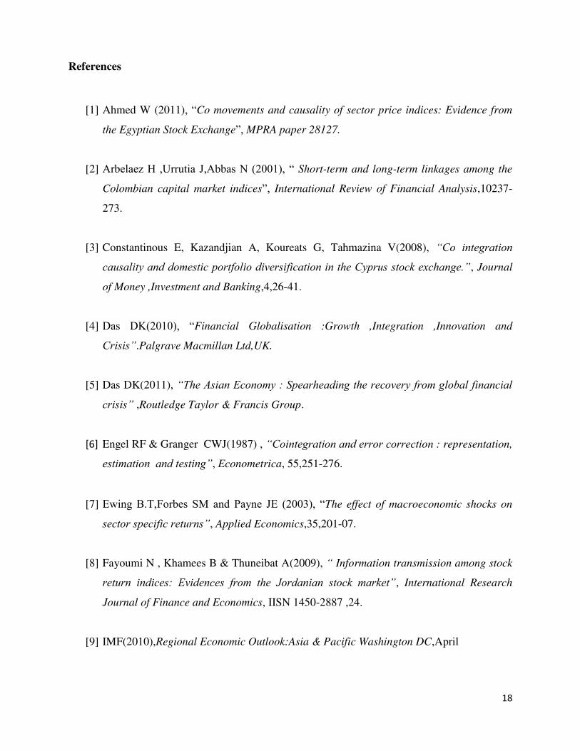
The two adjustment factors for the LBANKEX (-1) are:
α11=0.02877; the first adjustment factor associated the Cointegrating Equation (CE) makes it
move away in order to bring the system to equilibrium.
α12= 0.06264; the second adjustment factor for CE makes it move away faster from the system
(the speed of adjustment is larger for the 2nd adjustment factor α12) (Table 4 in Annexure)
The t-values for α11 and α12 are 1.68974 and 1.72494. As t 0.050,448 =1.645; these adjustment
coefficients are significant at 5% level of significance. LBankex with lag 1 responds to any
disequilibrium so as to come back to the equilibrium steady state.
The first co integrating vector’s normalized [for β11=1 ]
β'=[β11,β21,β31,β41,β51,β61,β71,β81] =[1.00, 0.00, 10.00, -1.909, -1.448, 0.5868, -3.174,-0.532]
These values represents the coefficients for LBANKEX (-1), LOILGAS (-1), LAUTO (-1), LCG (-1),
LMETAL (-1), LPOWER (-1), LREALTY (-1).
Thus, the first regression equation is represented by:
LBANKEX (-1) = -10.0056*LOILGAS (-1) + 1.9092*LAUTO (-1) +1.4476*LCG (-1)
+0.5867*LMETAL (-1) + 3.1741*LPOWER (-1) + 0.5320*LREALTY (-1) + 46.5961
Error Correction Term for D (LBANKEX)
The long-run coefficient matrix Π8x8 =αβ’ provides error correction terms which indicate
response from sector indices to adjust for achieving long-run equilibrium.
D (LBANKEX) represents growth in BANKEX
For D(LBANKEX) the error correction terms are represented in the regression model by
0.2119*D(LBANKEX(-1)) + 0.1712*D(LIT(-1)) + 0.1117*D(LOILGAS(-1)) -
0.0496*D(LAUTO(-1)) - 0.2237*D(LCG(-1)) - 0.1576*D(LMETAL(-1)) +
0.1652*D(LPOWER(-1)) - 0.0323*D(LREALTY(-1))
The coefficients of error correction terms for DLBANKEX are: [Π 11, Π 12, Π 13, Π 14,Π 15,Π 16,Π
17, Π 18].
The t-values for D(LBANKEX(-1),D(LIT(-1) ,D(LOILGAS(-1) , D(LCG(-1), D(LMETAL(-1),
D(LREALTY(-1) are > 1.96 implying these parameters are significant. Further, as calculated,
11
F=3.147500> F7, 448,10% = 1.72, therefore, reject the joint H0 : Π 1i =0 for all i. Thus, the 6
regressors jointly explain the long-term correction factor in D(LBANKEX) and the model is a
good fit.
The existence of cointegrating relationship signifies long-term relationship but due to this the
portfolio diversification benefits in long-run are not possible [Ahmed W (2011)]. However, as
seen that BANKEX is integrated with major sector indices, the policy for Bankex plays an
important role in the growth and controlling unexpected losses of other major sectors.
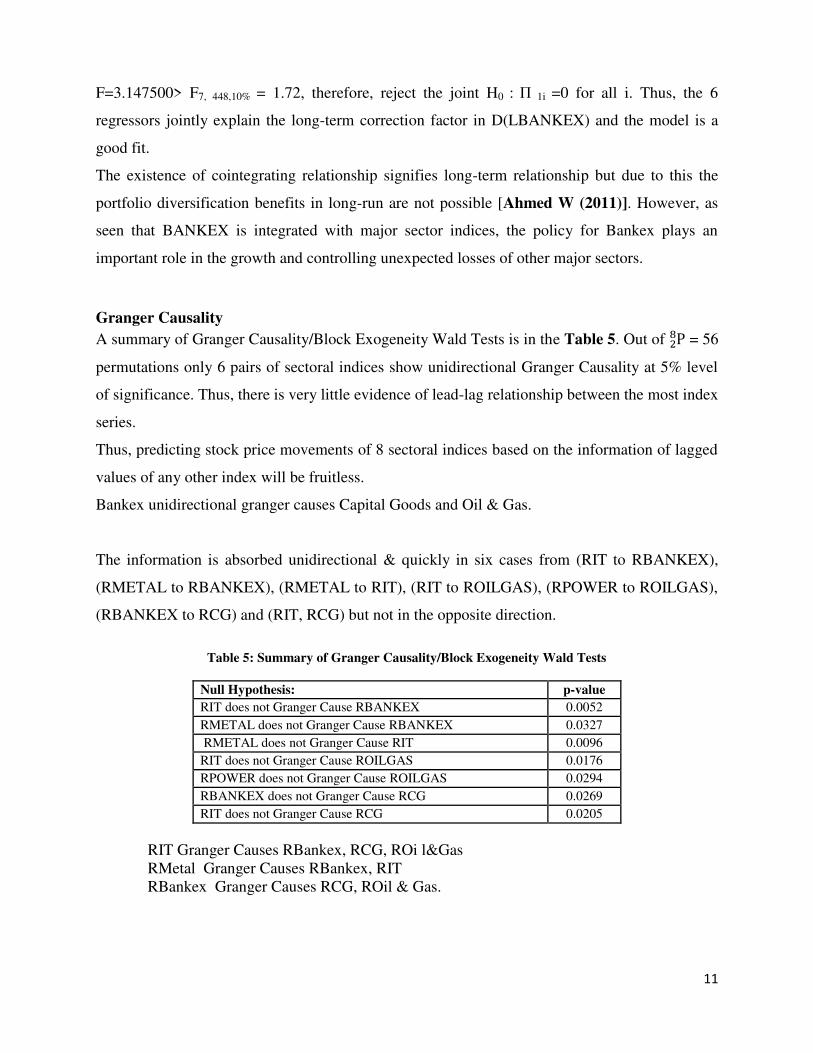
Granger Causality
A summary of Granger Causality/Block Exogeneity Wald Tests is in the Table 5. Out of = 56
permutations only 6 pairs of sectoral indices show unidirectional Granger Causality at 5% level
of significance. Thus, there is very little evidence of lead-lag relationship between the most index
series.
Thus, predicting stock price movements of 8 sectoral indices based on the information of lagged
values of any other index will be fruitless.
Bankex unidirectional granger causes Capital Goods and Oil & Gas.
The information is absorbed unidirectional & quickly in six cases from (RIT to RBANKEX),
(RMETAL to RBANKEX), (RMETAL to RIT), (RIT to ROILGAS), (RPOWER to ROILGAS),
(RBANKEX to RCG) and (RIT, RCG) but not in the opposite direction.
Table 5: Summary of Granger Causality/Block Exogeneity Wald Tests
Null Hypothesis: p-value
RIT does not Granger Cause RBANKEX 0.0052
RMETAL does not Granger Cause RBANKEX 0.0327
RMETAL does not Granger Cause RIT 0.0096
RIT does not Granger Cause ROILGAS 0.0176
RPOWER does not Granger Cause ROILGAS 0.0294
RBANKEX does not Granger Cause RCG 0.0269
RIT does not Granger Cause RCG 0.0205
RIT Granger Causes RBankex, RCG, ROi l&Gas
RMetal Granger Causes RBankex, RIT
RBankex Granger Causes RCG, ROil & Gas.
12
Thus, IT, Metal and Bankex are important for short-term upward movement of other sector
indices during the period of recovery.
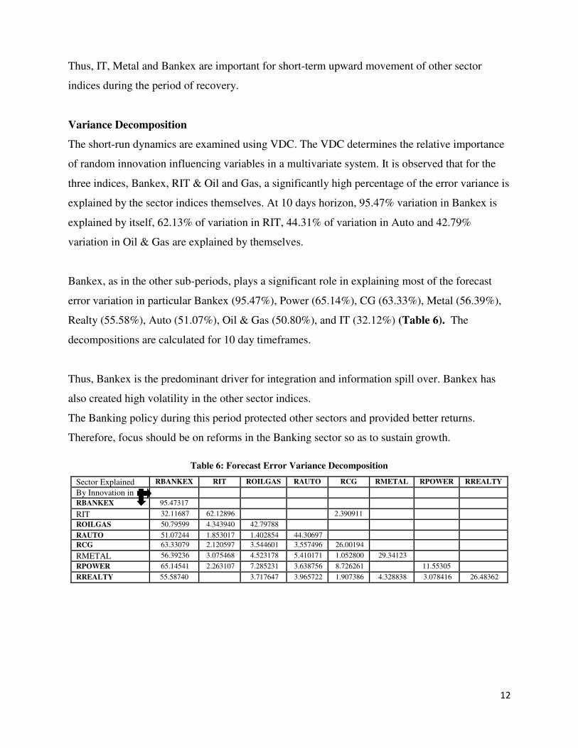
Variance Decomposition
The short-run dynamics are examined using VDC. The VDC determines the relative importance
of random innovation influencing variables in a multivariate system. It is observed that for the
three indices, Bankex, RIT & Oil and Gas, a significantly high percentage of the error variance is
explained by the sector indices themselves. At 10 days horizon, 95.47% variation in Bankex is
explained by itself, 62.13% of variation in RIT, 44.31% of variation in Auto and 42.79%
variation in Oil & Gas are explained by themselves.
Bankex, as in the other sub-periods, plays a significant role in explaining most of the forecast
error variation in particular Bankex (95.47%), Power (65.14%), CG (63.33%), Metal (56.39%),
Realty (55.58%), Auto (51.07%), Oil & Gas (50.80%), and IT (32.12%) (Table 6). The
decompositions are calculated for 10 day timeframes.
Thus, Bankex is the predominant driver for integration and information spill over. Bankex has
also created high volatility in the other sector indices.
The Banking policy during this period protected other sectors and provided better returns.
Therefore, focus should be on reforms in the Banking sector so as to sustain growth.
Table 6: Forecast Error Variance Decomposition
Sector Explained RBANKEX RIT ROILGAS RAUTO RCG RMETAL RPOWER RREALTY
By Innovation in
RBANKEX 95.47317
RIT 32.11687 62.12896 2.390911
ROILGAS 50.79599 4.343940 42.79788
RAUTO 51.07244 1.853017 1.402854 44.30697
RCG 63.33079 2.120597 3.544601 3.557496 26.00194
RMETAL 56.39236 3.075468 4.523178 5.410171 1.052800 29.34123
RPOWER 65.14541 2.263107 7.285231 3.638756 8.726261 11.55305
RREALTY 55.58740 3.717647 3.965722 1.907386 4.328838 3.078416 26.48362
13
Following is the summary of the analysis performed on the basis of (Table 6).
62.13% variation in IT is explained by itself, whereas, 32.12% by Bankex.
42.80% variation in Oil & Gas is explained itself, 50.80% variation in Oil and Gas by
Bankex and 4.34% is explained by IT.
44.30% variation in Auto is explained by itself, 51.07% variation in Auto is explained by
Bankex and 3.23% variation is explained jointly by IT & Oil & Gas.
26.00% variation in CG is explained by itself, whereas, 63.33% of its variation by Bankex
and 9.12 % variation is explained jointly by the three indices IT, Oil & Gas and Auto.
29.34 % variation in Metal is explained by itself, whereas, 56.39% by Bankex and remaining
by Auto (5.41%), Oil & Gas (4.52%) and IT (3.07%).
11.53% variation in Power is explained by itself, whereas, 65.14% of its variation is
explained by Bankex, 8.72% by CG and 7.28% by Oil and Gas.
26.48% variation in Realty is explained by itself and 55.59% of its variation is explained by
Bankex and 15.08% of variation is explained jointly by Metal, Auto, Oil & Gas and Power.
Generalized Impulse Response
The duration and response of effect of one standard deviation of innovation in one sector index
to the other sectoral indices is studied by Generalized Impulse Response Function (GIFR).
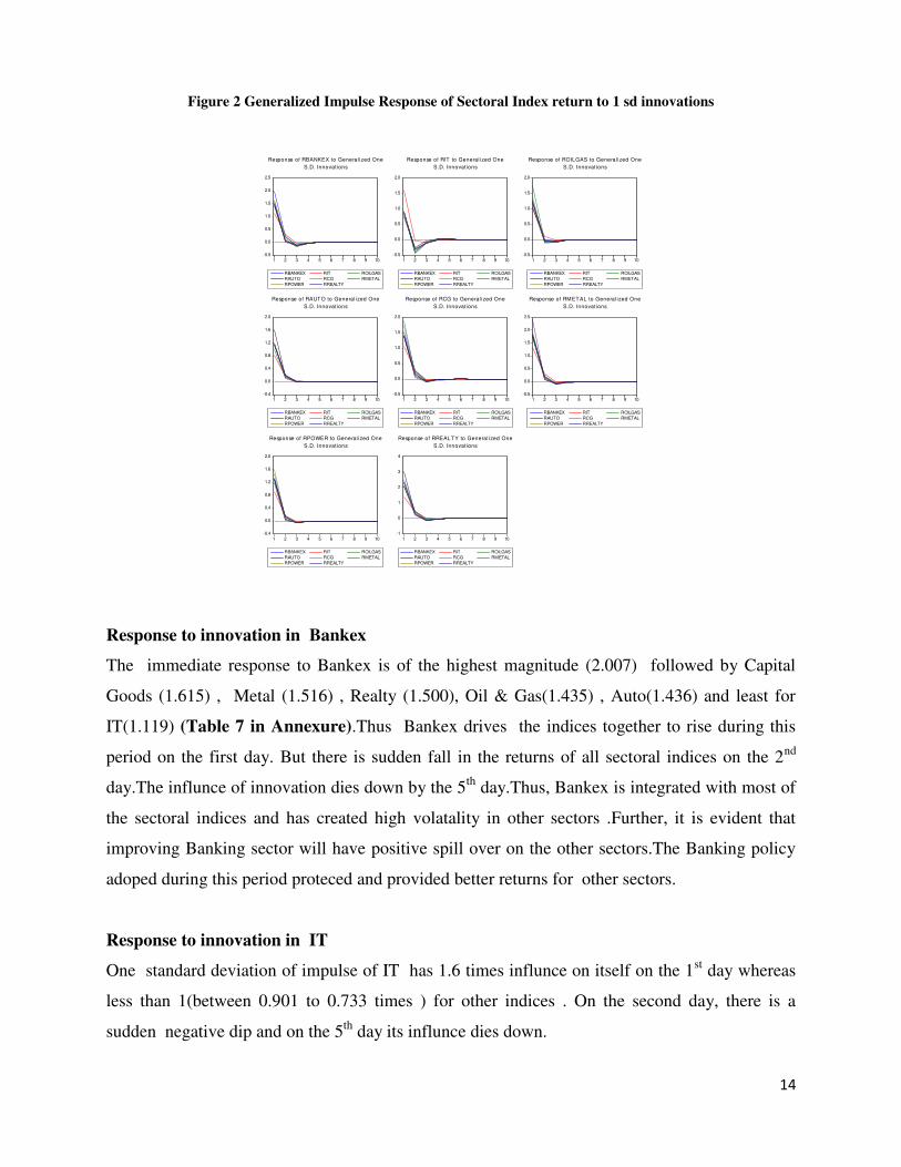
The Figure 2 presents response of sectoral indices to generalised one standard deviation
innovation. For each sectoral index there is a positive signifiacnt initial impact.It touches
negative value on 2nd
or 3rd
day for most indices and dies down quickly on the 5th
or 6th
day.
14
Figure 2 Generalized Impulse Response of Sectoral Index return to 1 sd innovations
Response to innovation in Bankex
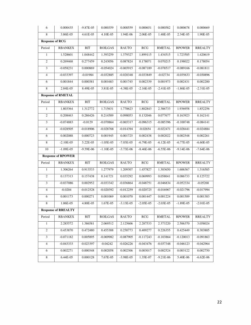
The immediate response to Bankex is of the highest magnitude (2.007) followed by Capital
Goods (1.615) , Metal (1.516) , Realty (1.500), Oil & Gas(1.435) , Auto(1.436) and least for
IT(1.119) (Table 7 in Annexure).Thus Bankex drives the indices together to rise during this
period on the first day. But there is sudden fall in the returns of all sectoral indices on the 2nd
day.The influnce of innovation dies down by the 5th
day.Thus, Bankex is integrated with most of
the sectoral indices and has created high volatality in other sectors .Further, it is evident that
improving Banking sector will have positive spill over on the other sectors.The Banking policy
adoped during this period proteced and provided better returns for other sectors.
Response to innovation in IT
One standard deviation of impulse of IT has 1.6 times influnce on itself on the 1st day whereas
less than 1(between 0.901 to 0.733 times ) for other indices . On the second day, there is a
sudden negative dip and on the 5th
day its influnce dies down.
-0.5
0.0
0.5
1.0
1.5
2.0
2.5
1 2 3 4 5 6 7 8 9 10
RBANKEX RIT ROILGAS
RAUTO RCG RMETAL
RPOWER RREALTY
Response of RBANKEX to General ized One
S.D. Innovations
-0.5
0.0
0.5
1.0
1.5
2.0
1 2 3 4 5 6 7 8 9 10
RBANKEX RIT ROILGAS
RAUTO RCG RMETAL
RPOWER RREALTY
Response of RIT to General ized One
S.D. Innovations
-0.5
0.0
0.5
1.0
1.5
2.0
1 2 3 4 5 6 7 8 9 10
RBANKEX RIT ROILGAS
RAUTO RCG RMETAL
RPOWER RREALTY
Response of ROILGAS to General ized One
S.D. Innovations
-0.4
0.0
0.4
0.8
1.2
1.6
2.0
1 2 3 4 5 6 7 8 9 10
RBANKEX RIT ROILGAS
RAUTO RCG RMETAL
RPOWER RREALTY
Response of RAUTO to General ized One
S.D. Innovations
-0.5
0.0
0.5
1.0
1.5
2.0
1 2 3 4 5 6 7 8 9 10
RBANKEX RIT ROILGAS
RAUTO RCG RMETAL
RPOWER RREALTY
Response of RCG to General ized One
S.D. Innovations
-0.5
0.0
0.5
1.0
1.5
2.0
2.5
1 2 3 4 5 6 7 8 9 10
RBANKEX RIT ROILGAS
RAUTO RCG RMETAL
RPOWER RREALTY
Response of RMETAL to General ized One
S.D. Innovations
-0.4
0.0
0.4
0.8
1.2
1.6
2.0
1 2 3 4 5 6 7 8 9 10
RBANKEX RIT ROILGAS
RAUTO RCG RMETAL
RPOWER RREALTY
Response of RPOWER to General ized One
S.D. Innovations
-1
0
1
2
3
4
1 2 3 4 5 6 7 8 9 10
RBANKEX RIT ROILGAS
RAUTO RCG RMETAL
RPOWER RREALTY
Response of RREALTY to General ized One
S.D. Innovations
15
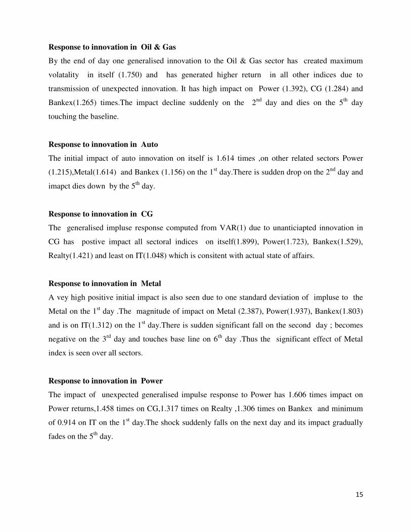
Response to innovation in Oil & Gas
By the end of day one generalised innovation to the Oil & Gas sector has created maximum
volatality in itself (1.750) and has generated higher return in all other indices due to
transmission of unexpected innovation. It has high impact on Power (1.392), CG (1.284) and
Bankex(1.265) times.The impact decline suddenly on the 2nd
day and dies on the 5th
day
touching the baseline.
Response to innovation in Auto
The initial impact of auto innovation on itself is 1.614 times ,on other related sectors Power
(1.215),Metal(1.614) and Bankex (1.156) on the 1st day.There is sudden drop on the 2
nd day and
imapct dies down by the 5th
day.
Response to innovation in CG
The generalised impluse response computed from VAR(1) due to unanticiapted innovation in
CG has postive impact all sectoral indices on itself(1.899), Power(1.723), Bankex(1.529),
Realty(1.421) and least on IT(1.048) which is consitent with actual state of affairs.
Response to innovation in Metal
A vey high positive initial impact is also seen due to one standard deviation of impluse to the
Metal on the 1st day .The magnitude of impact on Metal (2.387), Power(1.937), Bankex(1.803)
and is on IT(1.312) on the 1st day.There is sudden significant fall on the second day ; becomes
negative on the 3rd
day and touches base line on 6th
day .Thus the significant effect of Metal
index is seen over all sectors.
Response to innovation in Power
The impact of unexpected generalised impulse response to Power has 1.606 times impact on
Power returns,1.458 times on CG,1.317 times on Realty ,1.306 times on Bankex and minimum
of 0.914 on IT on the 1st day.The shock suddenly falls on the next day and its impact gradually
fades on the 5th
day.
16
Response to innovation in Realty
Highest impact is seen on all sector index returns due to unanticiapted genrealised impulse to
Realty.It is 3.058 times on itself,2.506 times on Power,2.287 times on Bankex and 2.069 times
on Oil and Gas.As in other cases it falls suddenly on the 2nd
day touches negative value on 3rd
day and dies down on the 6th
day.Thus there is high volatality due to impulse to the Realty which
triggers other sector contemporenously.
4. Conclusion
The line plots of log of the sectoral indices and Sensex for the period of recovery 10/03/2009 to
31/12/2010 shows an upward trend which gradually stabilizes making a uniform pattern.
Consumer Durables gave highest returns followed by Metal, Auto and Bankex whereas Oil &
Gas and Power registered low returns. The highest volatility of returns is for Oil & Gas followed
by Capital Goods, FMCG and Bankex and relatively low volatility was observed for Healthcare
and Auto sector. Sensex returns are highly positively correlated with the returns of Bankex,
Power, Capital Goods and Oil & Gas. Bankex index has strong relationship with Capital Goods
and Power index. The Johansen and Juselius (1990) multivariate cointegration analysis shows
existence of two cointegrating vector. Thus, the eight indices in the BSE share long-run
equilibrium, implying that the fluctuations in the prices in the near future could be predicted up
to some extent by using part of information provided by the other stock indices. The investors
with long holding period may get only moderate advantage from diversification strategy.
Another significant implication of existence of cointegration is that the different sectors of the
Indian capital market are influenced by the economic fundamentals which tend to bring these
sectoral indices together in the long-run.
No short-run Granger Causality/Block Exogeneity exists between sector indices during all sub-
periods indicating diversification opportunities for development of short-term investment
strategies in the BSE [Constantinou et al (2008)]. Thus, in most cases predicting stock price
movements of 8 sectoral indices based on the information of lagged values of any other index
will be fruitless. The investors with long holding period may get only moderate advantage from
the diversification strategy [Fayoumi et al. (2009), Sypriopoulos (2004)]. Thus, the inferences
are, in general, consistent with the economic theory that the capital market within Indian
economy have tendency to move in the same direction in the long-run [Ahmed W, (2011)].

17
Only 6 pairs of sectoral indices show unidirectional Granger Causality at 5% level of
significance. Thus, there is very little evidence of lead-lag relationship between the most index
series for short duration. Error variance decomposition analysis indicates that for three indices
Bankex, IT & Oil and Gas; a significantly high percentage of the error variance is explained by
the sector indices themselves. Bankex is the predominant driver for integration and information
spill over. Bankex is integrated with most of the sectoral indices and has created high volatility
in other sectors. The Banking policy followed by the government of India during this period
protected other sectors and provided better returns. Unanticipated innovation in CG has positive
impact on all sectoral indices. For Metal, a very high positive initial impact is seen due to one
standard deviation impulse to itself on the 1st day which is also observed for all other sector
indices. Due to unanticipated generalized impulse to Realty, highest impact is seen on all sector
index returns. It is 3.058 times on itself, 2.506 times on Power, 2.287 times on Bankex and 2.069
times on Oil and Gas. Thus, there is high volatility due to impulse to the Realty which triggers
other sectors contemporaneously. Hence, relevant policy for Metal and Realty sector would
protect average returns of the other sectors during the recessionary period.
Thus, during the post recessionary period majority of Indian sectors were protected and provided
marginally better returns due to focus on robust Banking policy. Realty & Metal were other
significant drivers influencing remaining sectors contemporaneously.
The results highlighted importance of usage of sector indices. The investors are not only
interested in the individual stock performance, but are also keen to know behavior of the
different sector indices which are used as a benchmark to evaluate performance of stocks and
portfolios. Our findings have implications for both investors and policy makers. The results
identify predominant drivers for different sector indices; determine significant causality linkages
and highlights opportunities for diversification for least integrated sectors.
18
References
[1] Ahmed W (2011), “Co movements and causality of sector price indices: Evidence from
the Egyptian Stock Exchange”, MPRA paper 28127.
[2] Arbelaez H ,Urrutia J,Abbas N (2001), “ Short-term and long-term linkages among the
Colombian capital market indices”, International Review of Financial Analysis,10237-
273.
[3] Constantinous E, Kazandjian A, Koureats G, Tahmazina V(2008), “Co integration
causality and domestic portfolio diversification in the Cyprus stock exchange.”, Journal
of Money ,Investment and Banking,4,26-41.
[4] Das DK(2010), “Financial Globalisation :Growth ,Integration ,Innovation and
Crisis”.Palgrave Macmillan Ltd,UK.
[5] Das DK(2011), “The Asian Economy : Spearheading the recovery from global financial
crisis” ,Routledge Taylor & Francis Group.
[6] Engel RF & Granger CWJ(1987) , “Cointegration and error correction : representation,
estimation and testing”, Econometrica, 55,251-276.
[7] Ewing B.T,Forbes SM and Payne JE (2003), “The effect of macroeconomic shocks on
sector specific returns”, Applied Economics,35,201-07.
[8] Fayoumi N , Khamees B & Thuneibat A(2009), “ Information transmission among stock
return indices: Evidences from the Jordanian stock market”, International Research
Journal of Finance and Economics, IISN 1450-2887 ,24.
[9] IMF(2010),Regional Economic Outlook:Asia & Pacific Washington DC,April
19
[10] Johansen & Juselius (1991), “Estimation and hypothesis testing of co integrating vectors
in Gaussian vector auto regression models” , Econometrica ,59,1551-1580.
[11] Johansen S & Juselius K (1991), “Maximum likelihood estimation and inference on
cointegration - with applications to the demand of money”, Oxford Bulletin of
Economics and Statistics, 52,169-210.
[12] Poshakwala S & Patra T (2008), “Long-run and short-run relationship between the
main stock indices: Evidence from Athens stock exchange”, Applied Financial
Economics, 2008, 18, 1401-1410.
[13] Sim CA,Stock JH and Watson MW (1990), “Inference in linear time Series models with
unit roots”,Econometrica, 58, 113-44.
[14] Syriopoulos ,T (2004) , “International Portfolio Diversification to central European
stock markets”, Applied Financial Economics .14,1253-1268.
[15] Wang Z,Kutan ,A and Yang,J(2005), “ Information within and across sectors in Chinese
Stock Markets”,The Quarterly Review of Economic and Finance,45,768-80.
[16] World Bank(2010), “ East Asia and Pacific Economic update”, May 2010.
20
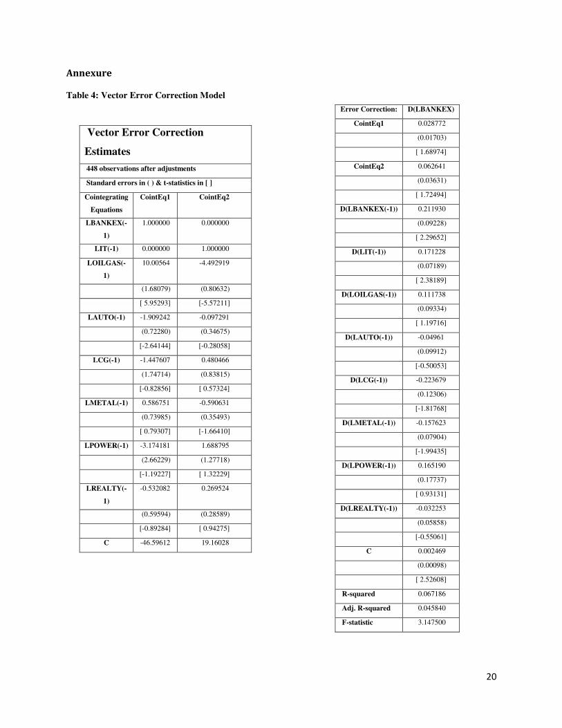
Annexure
Table 4: Vector Error Correction Model
Vector Error Correction
Estimates
448 observations after adjustments
Standard errors in ( ) & t-statistics in [ ]
Cointegrating
Equations
CointEq1 CointEq2
LBANKEX(-
1)
1.000000 0.000000
LIT(-1) 0.000000 1.000000
LOILGAS(-
1)
10.00564 -4.492919
(1.68079) (0.80632)
[ 5.95293] [-5.57211]
LAUTO(-1) -1.909242 -0.097291
(0.72280) (0.34675)
[-2.64144] [-0.28058]
LCG(-1) -1.447607 0.480466
(1.74714) (0.83815)
[-0.82856] [ 0.57324]
LMETAL(-1) 0.586751 -0.590631
(0.73985) (0.35493)
[ 0.79307] [-1.66410]
LPOWER(-1) -3.174181 1.688795
(2.66229) (1.27718)
[-1.19227] [ 1.32229]
LREALTY(-
1)
-0.532082 0.269524
(0.59594) (0.28589)
[-0.89284] [ 0.94275]
C -46.59612 19.16028
Error Correction: D(LBANKEX)
CointEq1 0.028772
(0.01703)
[ 1.68974]
CointEq2 0.062641
(0.03631)
[ 1.72494]
D(LBANKEX(-1)) 0.211930
(0.09228)
[ 2.29652]
D(LIT(-1)) 0.171228
(0.07189)
[ 2.38189]
D(LOILGAS(-1)) 0.111738
(0.09334)
[ 1.19716]
D(LAUTO(-1)) -0.04961
(0.09912)
[-0.50053]
D(LCG(-1)) -0.223679
(0.12306)
[-1.81768]
D(LMETAL(-1)) -0.157623
(0.07904)
[-1.99435]
D(LPOWER(-1)) 0.165190
(0.17737)
[ 0.93131]
D(LREALTY(-1)) -0.032253
(0.05858)
[-0.55061]
C 0.002469
(0.00098)
[ 2.52608]
R-squared 0.067186
Adj. R-squared 0.045840
F-statistic 3.147500
21
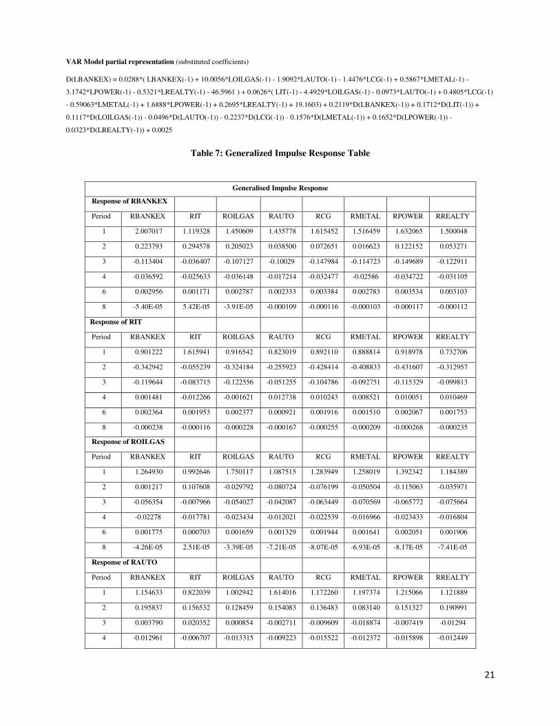
VAR Model partial representation (substituted coefficients)
D(LBANKEX) = 0.0288*( LBANKEX(-1) + 10.0056*LOILGAS(-1) - 1.9092*LAUTO(-1) - 1.4476*LCG(-1) + 0.5867*LMETAL(-1) -
3.1742*LPOWER(-1) - 0.5321*LREALTY(-1) - 46.5961 ) + 0.0626*( LIT(-1) - 4.4929*LOILGAS(-1) - 0.0973*LAUTO(-1) + 0.4805*LCG(-1)
- 0.59063*LMETAL(-1) + 1.6888*LPOWER(-1) + 0.2695*LREALTY(-1) + 19.1603) + 0.2119*D(LBANKEX(-1)) + 0.1712*D(LIT(-1)) +
0.1117*D(LOILGAS(-1)) - 0.0496*D(LAUTO(-1)) - 0.2237*D(LCG(-1)) - 0.1576*D(LMETAL(-1)) + 0.1652*D(LPOWER(-1)) -
0.0323*D(LREALTY(-1)) + 0.0025
Table 7: Generalized Impulse Response Table
Generalised Impulse Response
Response of RBANKEX
Period RBANKEX RIT ROILGAS RAUTO RCG RMETAL RPOWER RREALTY
1 2.007017 1.119328 1.450609 1.435778 1.615452 1.516459 1.632065 1.500048
2 0.223793 0.294578 0.205023 0.038500 0.072651 0.016623 0.122152 0.053271
3 -0.113404 -0.036407 -0.107127 -0.10029 -0.147984 -0.114723 -0.149689 -0.122911
4 -0.036592 -0.025633 -0.036148 -0.017214 -0.032477 -0.02586 -0.034722 -0.031105
6 0.002956 0.001171 0.002787 0.002333 0.003384 0.002783 0.003534 0.003103
8 -5.40E-05 5.42E-05 -3.91E-05 -0.000109 -0.000116 -0.000103 -0.000117 -0.000112
Response of RIT
Period RBANKEX RIT ROILGAS RAUTO RCG RMETAL RPOWER RREALTY
1 0.901222 1.615941 0.916542 0.823019 0.892110 0.888814 0.918978 0.732706
2 -0.342942 -0.055239 -0.324184 -0.255923 -0.428414 -0.408833 -0.431607 -0.312957
3 -0.119644 -0.083715 -0.122556 -0.051255 -0.104786 -0.092751 -0.115329 -0.099813
4 0.001481 -0.012266 -0.001621 0.012738 0.010243 0.008521 0.010051 0.010469
6 0.002364 0.001953 0.002377 0.000921 0.001916 0.001510 0.002067 0.001753
8 -0.000238 -0.000116 -0.000228 -0.000167 -0.000255 -0.000209 -0.000268 -0.000235
Response of ROILGAS
Period RBANKEX RIT ROILGAS RAUTO RCG RMETAL RPOWER RREALTY
1 1.264930 0.992646 1.750117 1.087515 1.283949 1.258019 1.392342 1.184389
2 0.001217 0.107608 -0.029792 -0.080724 -0.076199 -0.050504 -0.115063 -0.035971
3 -0.056354 -0.007966 -0.054027 -0.042087 -0.063449 -0.070569 -0.065772 -0.075664
4 -0.02278 -0.017781 -0.023434 -0.012021 -0.022539 -0.016966 -0.023433 -0.016804
6 0.001775 0.000703 0.001659 0.001329 0.001944 0.001641 0.002051 0.001906
8 -4.26E-05 2.51E-05 -3.39E-05 -7.21E-05 -8.07E-05 -6.93E-05 -8.17E-05 -7.41E-05
Response of RAUTO
Period RBANKEX RIT ROILGAS RAUTO RCG RMETAL RPOWER RREALTY
1 1.154633 0.822039 1.002942 1.614016 1.172260 1.197374 1.215066 1.121889
2 0.195837 0.156532 0.128459 0.154083 0.136483 0.083140 0.151327 0.190991
3 0.003790 0.020352 0.000854 -0.002711 -0.009609 -0.018874 -0.007419 -0.01294
4 -0.012961 -0.006707 -0.013315 -0.009223 -0.015522 -0.012372 -0.015898 -0.012449
22
6 0.000435 -9.87E-05 0.000359 0.000559 0.000651 0.000582 0.000678 0.000669
8 3.86E-05 4.61E-05 4.10E-05 1.94E-06 2.06E-05 1.48E-05 2.34E-05 1.90E-05
Response of RCG
Period RBANKEX RIT ROILGAS RAUTO RCG RMETAL RPOWER RREALTY
1 1.528601 1.048442 1.393259 1.379327 1.899115 1.434515 1.723505 1.420619
2 0.269468 0.277459 0.243056 0.087824 0.178071 0.070215 0.198022 0.178054
3 -0.058231 0.000869 -0.054024 -0.065915 -0.087189 -0.078517 -0.089166 -0.081811
4 -0.033397 -0.01984 -0.032885 -0.020348 -0.033849 -0.02734 -0.035633 -0.030896
6 0.001844 0.000381 0.001683 0.001745 0.002339 0.001973 0.002431 0.002200
8 2.84E-05 8.49E-05 3.81E-05 -4.38E-05 -2.16E-05 -2.41E-05 -1.86E-05 -2.31E-05
Response of RMETAL
Period RBANKEX RIT ROILGAS RAUTO RCG RMETAL RPOWER RREALTY
1 1.803364 1.312772 1.715631 1.770623 1.802843 2.386733 1.936958 1.852256
2 0.208463 0.286426 0.214589 0.098053 0.132046 0.077677 0.163923 0.162141
3 -0.074883 -0.0129 -0.070864 -0.065317 -0.096315 -0.085396 -0.100748 -0.084141
4 -0.028505 -0.018906 -0.028768 -0.014394 -0.02654 -0.022471 -0.028441 -0.024884
6 0.002088 0.000723 0.001945 0.001725 0.002438 0.002022 0.002548 0.002261
8 -2.10E-05 5.22E-05 -1.05E-05 -7.03E-05 -6.79E-05 -6.12E-05 -6.77E-05 -6.60E-05
10 -1.09E-05 -9.59E-06 -1.10E-05 -3.73E-06 -8.46E-06 -6.55E-06 -9.14E-06 -7.64E-06
Response of RPOWER
Period RBANKEX RIT ROILGAS RAUTO RCG RMETAL RPOWER RREALTY
1 1.306264 0.913533 1.277979 1.209307 1.457827 1.303650 1.606367 1.316585
2 0.137313 0.157438 0.141721 0.035292 0.069993 0.058041 0.086733 0.125722
3 -0.037086 0.002952 -0.033342 -0.036864 -0.048751 -0.046834 -0.052334 -0.05268
4 -0.0204 -0.012528 -0.020392 -0.012259 -0.020725 -0.016967 -0.021796 -0.017994
6 0.001173 0.000271 0.001069 0.001070 0.001447 0.001224 0.001509 0.001383
8 1.06E-05 4.80E-05 1.67E-05 -3.13E-05 -2.05E-05 -2.03E-05 -1.89E-05 -2.01E-05
Response of RREALTY
Period RBANKEX RIT ROILGAS RAUTO RCG RMETAL RPOWER RREALTY
1 2.285572 1.386581 2.069512 2.125606 2.287533 2.373220 2.506370 3.058024
2 0.453870 0.472480 0.455388 0.258773 0.409277 0.226355 0.425449 0.303805
3 -0.071182 0.005895 -0.069982 -0.087905 -0.117243 -0.103864 -0.120013 -0.091863
4 -0.043333 -0.023397 -0.04242 -0.026226 -0.043476 -0.037348 -0.046123 -0.042964
6 0.002271 0.000348 0.002058 0.002306 0.003017 0.002524 0.003122 0.002750
8 6.44E-05 0.000128 7.67E-05 -3.98E-05 1.35E-07 -9.21E-06 5.40E-06 -6.62E-06