Munich Personal RePEc Archive

Does quality influence choice of general

practitioner? An analysis of matched

doctor-patient panel data

Biorn, Erik and Godager, Geir

May 2008

Online at https://mpra.ub.uni-muenchen.de/8793/

MPRA Paper No. 8793, posted 20 May 2008 02:40 UTC

HERO

Does quality

influence choice of

general practitioner?

An analysis of

matched doctor-

patient panel data

Erik Biørn

Department of Economics,

University of Oslo

Geir Godager

Institute of Health Management

and Health Economics,

University of Oslo

Working paper 2008: 3

Does quality influence choice of general

practitioner?

An analysis of matched doctor-patient panel data

Erik Biørn

Department of Economics, University of Oslo

Geir Godager

Institute of Health Management and Health Economics, University of Oslo

Health Economics Research Programme at the University of Oslo

HERO 2008

© 2008 HERO and the authors – Reproduction is permitted when the source is referred to.

Health Economics Research Programme at the University of Oslo.

Financial support from The Research Council of Norway is acknowledged.

ISSN 1501-9071 (print version.), ISSN 1890-1735 (online), ISBN 82-7756-186-5

DOES QUALITY INFLUENCE CHOICE OF GENERAL PRACTITIONER?

AN ANALYSIS OF MATCHED DOCTOR-PATIENT PANEL DATA

ERIK BIØRN

Department of Economics, University of Oslo,

P.O. Box 1095 Blindern, 0317 Oslo, Norway

E-mail: erik.biorn@econ.uio.no

GEIR GODAGER

Institute of Health Management and Health Economics, University of Oslo,

P.O. Box 1089 Blindern, 0317 Oslo, Norway

E-mail: g.c.godager@medisin.uio.no

Abstract: The impact of quality on the demand facing health care providers has importantimplications for the industrial organization of health care markets. In this paper we study theconsumers’ choice of general practitioner (GP) assuming they are unable to observe the truequality of GP services. A panel data set for 484 Norwegian GPs, with summary information ontheir patient stocks, renders the opportunity to identify and measure the impact of GP quality onthe demand, accounting for patient health heterogeneity in several ways. We apply modeling andestimation procedures involving latent structural variables, inter alia, a LISREL type of model,is used. The patient excess mortality rate at the GP level is one indicator of the quality. Weestimate the effect of this quality variable on the demand for each GP’s services. Our results,obtained from two different econometric model versions, indicate that GP quality has a clearpositive effect on demand.

Keywords: GP services. Health care quality. Health care demand. Latent variables. LISREL.Panel data. Norway

JEL classification: C23, C33, D83, H51, H75, I11, I18

Acknowledgements: We are grateful for comments from Tor Iversen, Karin Monstad, IsmoLinnosmaa, Terje Skjerpen and participants at the 27th Nordic Health Economists Study GroupMeeting, Copenhagen, August 2006, a Workshop on Health Economics, Oslo, August 2006, andthe 6th iHEA World Congress in Health Economics, Copenhagen, July 2007. Financial supportfrom the Norwegian Ministry of Health and Care Services and the Research Council of Norway isacknowledged. Some of the data applied are provided by the National Insurance Administrationand Statistics Norway and have been prepared for research purposes by The Norwegian SocialScience Data Services. The authors alone are responsible for all analyses and interpretations.

1 Introduction

Asymmetric information between physicians and their patients is a basic characteristic

of the market for health care services. In the words of Arrow (1963):

“...medical knowledge is so complicated, the information possessed by the physician

as to the consequences and possibilities of treatment is necessarily very much greater

than that of the patient, or at least so it is believed by both parties”.

Patients are therefore often considered to be poor judges of service quality. However,

those who have repeated encounters with the same health care provider, will accumulate

information on services and treatment outcomes, thus narrowing the information gap.

The market for general practitioners’ services is characterized by durable doctor-patient

relations that may improve the patients’ quality assessment. The aim of this paper is to

investigate empirically whether the demand facing a general practitioner (GP) responds

to the quality of the provided services.

General background

The impact of quality on the demand facing health care providers has important im-

plications for the organization of health care markets. There is a growing literature on

competition and quality in such markets, from which an important result is that the

effect of stronger competition on quality depends crucially on the relative sizes of the

price elasticity and the quality elasticity of demand. More competition may bring about

reductions in quality if the quality elasticity is small compared to the price elasticity

(Dranove and Satterthwaite, 2000, Gaynor, 2006). Further, the impact of quality on the

demand facing health care providers has important implications for the optimal design of

payment systems. A familiar result is that a retrospective payment scheme in the form of

cost reimbursement is likely to pursue the goal of quality provision while giving weak in-

centives to provide cost reducing efforts. Conversely, prospective payment schemes tend

to strengthen the incentives for cost reduction, while weakening the incentives for provid-

ing quality. A combination of payment mechanisms is thus likely to perform better than

payment systems employing only one parameter. However, if quality affects demand, a

first-best solution can, in theory, be obtained under a pure prospective payment scheme

(Ma, 1994). This suggests that the effect of quality on demand – and information on its

numerical size – is a key factor determining the optimal calibration of the parameters in

the payment system: If the market punishes providers who are skimping on quality, the

payment system can put more weight on the parameters that encourage cost reducing

efforts.

Relation to literature

A conventional empirical approach when seeking to assess the effect of quality on demand

for health services is to estimate the effect of provider characteristics on individual con-

1

sumers’ choice of provider, applying different models for individuals’ discrete choice. An

influential paper in this tradition is Luft et al. (1990). They specifically study the effect

of quality indicators such as death and complication rates, teaching status of hospital,

and out of state admissions on patients’ choice of hospital, using logit models, and find

positive effects for several of the applied indicators. Using similar quality indicators and

methods, Burns and Wholey (1992) extend the framework by including in their logit

models characteristics of the admitting physician. They find that quality affects demand

positively, and that characteristics of the admitting physician are important determinants

of patients’ hospital choice. More recently, Howard (2005), applying a mixed logit model

on data on kidney transplantations, estimated the effect of the deviation from expected

failure rate on probabilities of hospital choice. The results indicate that hospitals with

a higher than expected failure rate have smaller probabilities for being chosen. A differ-

ent empirical strategy is followed in Chirikos (1992), in estimating, by linear regression,

the effect of individual hospitals’ quality spending on their market shares. The results

support the hypothesis that increased provider quality affects demand positively.

The present paper adds to the literature in several ways. First, no previous empirical

studies seem to have considered the demand effects of quality in the market for general

practitioners. Second, in the current literature the relationship between demand and

various indicators of quality, such as mortality rates, failure rates or hospital type, and

other independent variables, are estimated separately. The present paper contributes to

the literature by simultaneously estimating the relationship between demand and several

quality indicators, applying linear structural equation modeling (LISREL) and estimation

methods. Within this framework we acknowledge both the multidimensional aspect of the

quality concept, and that it may be considered as more appropriate to interpret outcome

measures such as mortality rates or failure rates as functions of quality, rather than as

measuring quality itself. Third, our econometric model has a wider field of application

as it provides a method to separate the effect of quality on outcome measures from the

effect of patient health.

Setting of the study

In June 2001 a regular GP scheme was introduced in Norwegian general practice, making

the GPs responsible for the provision of primary care services to the persons listed at

their practice. Prior to the reform the health authorities gathered the information needed

to assign one GP to each Norwegian inhabitant. All inhabitants were asked to rank their

three most preferred GPs in a form, and all GPs were asked to report the maximum

number of patients they would like to take care of. An algorithm was designed to utilize

this information and obtain a one-to-one match between inhabitants and GPs.

Our data set has a panel format with the GP as the observation unit, but for some

variables only one observation per GP exists. The data stem from The Norwegian General

Practitioners Database, covering all Norwegian GPs, supplemented by measures of the

2

GP density in each municipality and of age-gender specific mortality rates. Among

the variables recorded are the number of persons who ranked each GP as most preferred

when returning the entry form, the number of mortalities among each GP’s listed patients

during a six-month period, and the proportion of the listed persons who switch to other

GPs in later periods. For a stratified sample of GPs, relating to 14 municipalities, from

this official GP database the data set has been extended to also include the median income

and wealth of the listed persons and the proportion of them who have not finished high-

school. In the analysis, we interpret the number of first-rankings and the proportion of

listed persons who switch to other GPs, as indicators of the demand facing each GP.

Our main hypothesis is that there exists a latent stochastic variable, denoted as GP

quality, which, when heterogeneity related to the health status of the listed persons and

other observed heterogeneity have been accounted for, is positively related to the demand

facing each individual GP and negatively related to the recorded excess mortality of the

GP’s listed patients. We find empirical support to this hypothesis.

Two kinds of models are considered: a Panel Data model with latent heterogeneity

related to perceived GP quality and a multi-equation LISREL type of model, including

both GP quality and the health of the stock of persons on the GP’s list as latent variables,

both of which are assumed to affect demand as well as other observed variables. For some

variables, including the proportion of persons switching and the excess mortality, we have

data in the panel data format. This is profitable for quantifying the latent heterogeneity

and its consequences.

The rest of the paper proceeds as follows. The modeling of the demand in the market

for GPs is discussed in the following two sections. In Section 2, we present a theoretical

argument supporting the view that the expected demand facing each individual GP

can be a function of quality, even if the true quality is unobserved to his/her potential

patients. The discussion motivates testable predictions and hypotheses to be examined in

the paper. In Section 3, we present the two econometric models. The data are described

in Section 4, while estimation and test results are presented in Section 5. In Section 6

we discuss the results and conclude.

2 A model of patients’ quality perceptions

and demand for GPs

Quality and demand

In order to model the consumers’ choice of GP when they are unable to observe the

true quality of GP services, we first show that if the errors in the quality assessment of

potential patients have certain properties, the demand for GPs will depend on quality

even when the latter is unobservable. Consumers are imperfectly informed about the

quality of GPs and we therefore distinguish between true and perceived quality. We

3

assume that the only criterion for selecting a GP is the perceived quality of the services

provided. Quality of health care services is a complex entity that is not easily represented

by a scalar measure. In this model, however, quality can (in principle) be quantified and

completely described by a number on a finite scale. One may thus think of quality as

an input factor in the GP’s ‘health production function’. While predetermined abilities,

such as individual talent, obviously influence quality, the GP also has discretionary power

to influence quality by the exertion of ‘quality generating efforts’, such as concentration.

The individual GP’s quality of services is determined by his/her abilities and preferences

and we assume that the latter are both time invariant, implying that quality also is time

invariant.

The consumer’s information set is comprised by quantitative information on the qual-

ity of each available GP. This information, however, is ‘contaminated’ by stochastic errors.

The quality of GPs as perceived by a consumer may be higher or lower than the true

quality, and two consumers are likely to have different beliefs regarding the quality of

the same GP. The stochastic properties of what we may think of as measurement er-

rors drive the matching of consumers and GPs in the model. Let µj denote the true

quality of GP j (j = 1, . . . , M), while qij denotes the quality of GP j as perceived by

consumer i (i = 1, . . . , N). We assume that qij is normally distributed with E(qij) = µj

and var(qij) = σ2j , i.e., the distribution of the perceived quality differs between GPs. We

thus allow for the possibility that the population of consumers may have more accurate

information about GPs who have been active in the market for a long time (low σ2j ) com-

pared to GPs who have established their practice recently (high σ2j ). We let uij = qij−µj

and assume that the MN uijs are uncorrelated both across GPs and over consumers.

Altogether, we can therefore state our assumptions as

(1)qij = µj + uij ,

uij ∼ N(0, σ2j ), E(uijulk) = 0, i 6= l or j 6= k,

i, l = 1, . . . , N,j, k = 1, . . . , M.

We simply assume that consumer i considers perceived quality qij as indicating the

true quality of GP j. Since the normal distribution has an infinite support, the distri-

bution of perceived qualities associated with the GPs with the highest and the lowest

true quality overlap. This ensures that even if µj < µk, there is a positive probability

that qij >qik, so that any GP has a strictly positive probability of being selected by any

consumer. This implication seems reasonable if the differences in true quality is not too

large.

Matching GPs and consumers

We may think of the matching of GPs and consumers as a lottery. A draw is a realization

of qi1, qi2, . . . , qiM , that is, the realizations of the beliefs of the quality of each and one

of the GPs for consumer i. There are thus N independent drawings performed in the

market, one for each consumer. Let φ(qij ; µj , σ2j ) denote the density function of qij , the

4

perceived quality of GP j, which according to (1) is distributed as N(µj , σ2j ). To simplify

notation we let ∆ijk = qij − qik be the difference between consumer i’s perceived quality

of GPs j and k. It follows from (1) that ∆ijk ∼ N(νjk, θ2jk), with density function

φ(∆ijk; νjk, θ2jk), where

(2) νjk = µj−µk, θ2jk = σ2

j + σ2k, j, k = 1, . . . , M.

Let Ajk denote the event that ∆ijk > 0 for an arbitrary consumer, i. Then

(3) P (Ajk) = P (∆ijk > 0) =∫ ∞

0 φ(∆ijk; νjk, θ2jk)d∆ijk ≡ pjk

is the probability that GP j has a higher perceived quality than GP k. Since the draws

are assumed to be independent, the event that GP j has the highest perceived quality in

a random draw can thus be expressed as

Bj =M⋂

k=1k 6=j

Ajk, j =1, . . . , M.

The probability of this event can be expressed as:

(4) P (Bj) = P (∆ijk >0; ∀k 6=j)=M∏

k=1k 6=j

pjk ≡ πj , j =1, . . . ,M.

The probability that GP j has the highest perceived quality in a draw, πj , is a function of

µ1, . . . , µM ; σ21, . . . , σ

2M . Since (3) implies that ∂ pjk/∂νjk > 0 ∀ j 6= k, it follows from (2)

and (4) that ∂πj/∂µj > 0 and ∂πj/∂µk < 0, k 6= j. Hence, for all GPs, the probability

of being selected by any consumer is an increasing function of the true quality. When

consumers select the GP with the highest perceived quality, the expected demand facing

GP j is πjN . The expected demand facing any GP therefore changes in proportion to

the number of consumers in the market. Or stated otherwise, the probability of being

selected by a random consumer can be interpreted as the GP’s expected market share.

The ex-post market share converges to the probability of being selected by a random

consumer as the number of drawings increases.

From this model we can make the following predictions:

[P1] GPs with high quality of services have a higher probability of being selected by a randomly

chosen consumer than a GP whose services are of lower quality.

[P2] The selection probabilities πj are independent of the number of consumers, N . For a given

population of M GPs, expected demand for the services of any of them, is a linear function of N .

This, rather simple, model implies that the consumers are unable to affect the preci-

sion of their own quality assessment, reflected by the assumption that perceived quality

of GP j has the same variance, σ2j , for all consumers. The model could be generalized

to allow for consumer heterogeneity in the sense that some are more skillful or eager in

gathering and processing information in the market than others. This could have been

5

accounted for by replacing σ2j by σ2

ij , where σ2ij <σ2

hj if consumer i has taken efforts to

become better informed about GP j’s quality than has consumer h. A prediction from

such an extended model may be that high-quality GPs tend to have a higher proportion

of skilled or eager consumers on their lists than the low-quality GPs (Godager, 2008).

The possible existence of such a selection mechanism is important since consumers who

are skilled or eager in collecting information, may have a health status and a death

probability different from those not so skilled or eager.

The crucial question then becomes: which groups of consumers, according to ob-

servable characteristics, devote most attention and efforts in searching for the best GP?

On the one hand, less healthy consumers, with a high expected mortality rate, may be

thought to be particularly concerned about their choice of GP and as a result be more

willing to collect information than the average consumer. This may contribute to in-

creasing the average mortality rate among the patients listed with high-quality GPs. On

the other hand, consumers who are more healthy and resourceful and have low expected

mortality may be particularly able to collect and process such information. This may

contribute to the outcome of the selection mechanism being reversed, i.e., lowering the

average mortality rates of the persons listed with high-quality GPs. Consequently, from

a priori reasoning it is not obvious that the outcome of (observed or unobserved) pa-

tient heterogeneity will be neither that high-quality GPs attract patients with an average

health status which differs from that of the low-quality GPs, nor if there is a difference, in

which direction it will go. If a mechanism systematically selecting patients with different

expected mortality rates for GPs of different professional quality is at work, and hetero-

geneity in health status among listed patients is not taken care of in our modelling, we

are likely to face severe difficulties when trying to estimate the impact on demand of GP

service quality. The models to be described below have different degree of sophistication

and are not equally well designed to meet this challenge. We address this issue in more

detail in sections 3 and 5.

In elaborating the theory element above, we, for simplicity, have considered the con-

sumers’ mean perceived quality of GP j, µj , as non-stochastic. This interpretation is

provisional and intended to be valid only in a conditional sense. When, in the following,

this theory element will be embedded in an econometric model involving both latent and

observed variables related to GP quality, this variable will change its status and become

a latent, stochastic variable.

3 Econometric models

Motivation

In order to represent, and hopefully quantify, how the demand for GP services responds

to GP quality and other relevant variables – as motivated by the theoretical argument put

6

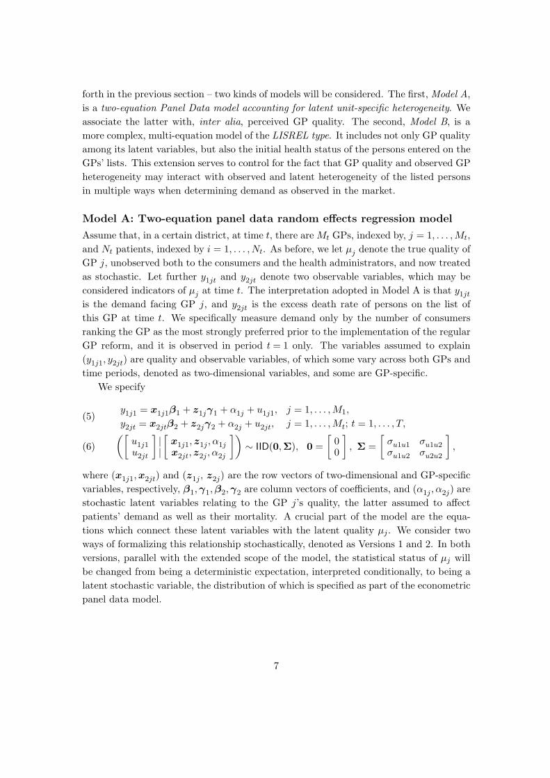
forth in the previous section – two kinds of models will be considered. The first, Model A,

is a two-equation Panel Data model accounting for latent unit-specific heterogeneity. We

associate the latter with, inter alia, perceived GP quality. The second, Model B, is a

more complex, multi-equation model of the LISREL type. It includes not only GP quality

among its latent variables, but also the initial health status of the persons entered on the

GPs’ lists. This extension serves to control for the fact that GP quality and observed GP

heterogeneity may interact with observed and latent heterogeneity of the listed persons

in multiple ways when determining demand as observed in the market.

Model A: Two-equation panel data random effects regression model

Assume that, in a certain district, at time t, there are Mt GPs, indexed by, j = 1, . . . ,Mt,

and Nt patients, indexed by i = 1, . . . , Nt. As before, we let µj denote the true quality of

GP j, unobserved both to the consumers and the health administrators, and now treated

as stochastic. Let further y1jt and y2jt denote two observable variables, which may be

considered indicators of µj at time t. The interpretation adopted in Model A is that y1jt

is the demand facing GP j, and y2jt is the excess death rate of persons on the list of

this GP at time t. We specifically measure demand only by the number of consumers

ranking the GP as the most strongly preferred prior to the implementation of the regular

GP reform, and it is observed in period t = 1 only. The variables assumed to explain

(y1j1, y2jt) are quality and observable variables, of which some vary across both GPs and

time periods, denoted as two-dimensional variables, and some are GP-specific.

We specify

y1j1 = x1j1β1 + z1jγ1 + α1j + u1j1, j = 1, . . . , M1,

y2jt = x2jtβ2 + z2jγ2 + α2j + u2jt, j = 1, . . . , Mt; t = 1, . . . , T,(5)

([u1j1u2jt

]||

[x1j1, z1j , α1jx2jt, z2j , α2j

])∼ IID(0,Σ), 0 =

[00

], Σ =

[σu1u1 σu1u2σu1u2 σu2u2

],(6)

where (x1j1, x2jt) and (z1j , z2j) are the row vectors of two-dimensional and GP-specific

variables, respectively, β1, γ1, β2, γ2 are column vectors of coefficients, and (α1j , α2j) are

stochastic latent variables relating to the GP j’s quality, the latter assumed to affect

patients’ demand as well as their mortality. A crucial part of the model are the equa-

tions which connect these latent variables with the latent quality µj . We consider two

ways of formalizing this relationship stochastically, denoted as Versions 1 and 2. In both

versions, parallel with the extended scope of the model, the statistical status of µj will

be changed from being a deterministic expectation, interpreted conditionally, to being a

latent stochastic variable, the distribution of which is specified as part of the econometric

panel data model.

7

Latent heterogeneity. Version 1: We first specify

α1j = λ1µj + ε1j ,

α2j = λ2µj + ε2j ,(7)

µjε1j

ε2j

|||

[x1j1,z1jx2jt, z2j

] ∼ IID(0,Ω), 0 =

000

, Ω =

[σ2

µ 0 00 σε1ε1 σε1ε20 σε2ε1 σε2ε2

],(8)

where we expect λ1 >0, λ2 <0, and σε1ε2 = σε2ε1 < 0. When µj is low, i.e., when GP j is

a low-quality doctor, then his/her patients will have a higher mortality rate than can be

explained by (x2jt, z2j), and he/she will meet a lower demand than can be explained by

(x1j1, z1j). Equations (5) and (7) define a four-equation system of structural equations

explaining (y1j1, y2jt, α1j , α2j) by (x1j1, x2jt, z1j , z2j , µj) and noise terms. Inserting (7)

into (5) yields the reduced form

(9)y1j1 = x1j1β1 + z1jγ1 + λ1µj + ε1j + u1j1, j = 1, . . . , M1,

y2jt = x2jtβ2 + z2jγ2 + λ2µj + ε2j + u2jt, j = 1, . . . , Mt; t = 1, . . . , T,

Latent heterogeneity. Version 2: The alternative version is

α1j = λα2j + εj ,(10)([

α2jεj

]||

[x1j1, z1jx2jt, z2j

])∼ IID

([00

],

[σ2

α2 00 σ2

ε

]),(11)

where we expect λ<0. Equations (5) and (10) define a three-equation system of structural

equations which explains (y1j1, y2jt, α1j) by (x1j1, x2jt, z1j , z2j , α2j) and noise terms. In-

serting (10) into (5) we get, instead of (9), the reduced form

(12)y1j1 = x1j1β1 + z1jγ1 + λα2j + εj + u1j1, j = 1, . . . , M1,

y2jt = x2jtβ2 + z2jγ2 + α2j + u2jt, j = 1, . . . , Mt; t = 1, . . . , T.

The latter equations, with λ = λ1/λ2 and εj = ε1j − λε2j , could, of course, alternatively

have been derived from (5) and (7). However, when (8) holds, (12) is not a reduced form,

since α2j is correlated with ε2j and therefore with the composite disturbance in the cross

section equation in (12), εj + u1j1.

The basic differences between the two model versions can be explained as follows:

First, it follows from (7) and (8) that Version 1 implies

(13) E

[α2

1j α1jα2j

α2jα1j α22j

]|||

[x1j1, z1j

x2jt, z2j

] =

[λ2

1σ2µ + σε1ε1 λ1λ2σ

2µ + σε1ε2

λ2λ1σ2µ + σε2ε1 λ2

2σ2µ + σε2ε2

],

and cov(αij , εkj) = σεiεk (i = 1, 2; k = 1, 2), which violate (10)–(11). Second, while

Version 1 treats latent quality µj as a symmetric ‘causal factor’ for y1j1 and y2jt, Version 2,

8

by treating α2j as the latent causal factor, introduces an asymmetry in the way quality

affects latent GP-specific heterogeneity in the two equations in (12).

The empirical implementation of Model A, to be presented in Section 5, relies on

Version 2, in that estimation is done sequentially and a predicted value of α2j obtained

from the second equation in (12), the excess mortality equation, serves as a proxy for

GP quality in the first equation, the demand equation. The estimators used in Section 5

may thus be consistent in Version 2, but inconsistent in Version 1.

Model B: LISREL model with GP quality and patient health latent

Model A gives a rather restrictive, uni-directional description of how demand for GP

services is related to GP quality. A LISREL model, i.e., a linear multi-equation structural

model with both manifest and latent structural variables may be a better solution to the

problem of modeling sample separation. Model B, now to be described, belongs to this

class. See Goldberger (1972), Joreskog (1977), Aigner et al. (1984, Sections 4 and 5),

and Joreskog et al. (2000) for further discussion of LISREL models.

Again, we exploit the panel design of our data set, with the GP as the observational

unit, containing GP-specific time-series for some variables, including patient-switching

and mortality rates, as well as GP-specific and patient specific time invariant variables.

We let t be the time index and suppress the GP subscript. Boldface and slim letters de-

note matrices/vectors and scalars, respectively. Model B has three categories of variables:

observable (manifest) structural variables, latent structural variables, and error/noise

variables. In the baseline version of the model, the categorization of the variables –

corresponding to the standard notation for latent and manifest variables in the LISREL

documentation – is as follows:

Observable (manifest) structural variables:y1: Number of persons wanting to be entered on list initially, in period 1 (scalar)

y2t: Number of persons switching to another GP in period t (scalar)

x1: Observed GP characteristics initially, in period 1 [(6×1)-vector]

x2: Observed patient characteristics initially, in period 1 [(3×1)-vector]

x3t: Excess mortality of patient stock in period t (scalar)

x4: Other time-invariant GP-characteristics unrelated to GP quality [(2×1)-vector]

y2≡ [y21, . . . , y2T ]′

x3 ≡ [x31, . . . , x3T ]′

Latent structural variables:η1: Demand directed towards GP (latent, time-invariant scalar)

ξ1: GP quality (latent, time-invariant scalar)

ξ2: Patient health (latent, time-invariant scalar)

ξ3≡ x4: Technical redefinition1

1 This redefinition is motivated by the fact that LISREL does not allow x variables to affect the η

variables directly in cases where the model also include ξ variables.

9

Error/noise variables:

ζ1: Disturbance in demand function

ε1, ε2t: Errors in the measurement equations for demand

δ1: Errors in equations relating GP quality to GP characteristics [(6×1)-vector]

δ2: Errors in equations relating patient health to patient characteristics. [(3×1)-vector]

δ3t: Errors in equations relating patient health and GP quality to excess mortality (scalar)

δ3 ≡ [δ31, . . . , δ3T ]′

ε2 ≡ [ε21, . . . , ε2T ]′

A basic hypothesis of the baseline version of Model B is that GP quality, ξ1, and

patient health status, ξ2, both time invariant scalars, are exogenous to the rest of the

system. The quality variable ξ1 corresponds to the variable µj in Model A, Version 1.

Time invariance and exogeneity are also assumed for the time invariant GP character-

istics, x4 = ξ3, in the model represented by the gender and the country of origin of the

GP; see below. These four variables are considered as determined from outside, inher-

ent in the GP and in the patient, and hence are not subject to feedback from the rest

of the system. This is an important assumption, which, for at least ξ1 and ξ2, may

be questioned. To some extent it will be modified later on (Section 5), in examining

the robustness of the primary conclusions concerning the link between GP quality and

patient demand to changes in basic assumptions. These genuinely exogenous variables

are, in the baseline model, indicated by observable ‘counterparts’, which, by assumption,

become endogenous.

The baseline model has four elements: (i) a demand function for GP services expressed

in terms of latent variables, (ii) measurement equations indicating this latent demand,

(iii) measurement equations indicating GP quality and health status of listed persons, and

(iv) distributional assumptions for the latent exogenous variables and the error terms.

First, the baseline version of the demand function, relating latent demand (endoge-

nous) to GP quality (exogenous), and latent health status and other characteristics of

the listed persons (all exogenous), is:

(14) η1 = Γ11ξ1 + Γ12ξ2 + Γ13ξ3 + ζ1 = [ Γ11 Γ12 Γ13 ]

ξ1

ξ2

ξ3

+ ζ1.

We can interpret Γ11,Γ12,Γ13 as (vectors of) structural coefficients and ζ1 as a distur-

bance.

Second, the baseline version of the measurement system for latent demand is

(15)

[y1

y2

]=

[ΛY 11

ΛY 21

]η1 +

[ε1

ε2

].

This subsystem expresses that y1, y21, . . . ,y2T are treated as T +1 observable indicators

of the latent demand for GP services. Technically, in factor-analytic terminology, we

10

can interpret ΛY 11 and ΛY 21 as factor loadings for, respectively, the number of persons

wanting to be on the list initially (positive loading) and the number of persons switching

to another GP in a later period (negative loading), on latent demand. In standard

regression terminology, we can interpret ΛY 11 and ΛY 21 as the marginal effects of the

latent variables on the corresponding observable variables. The error terms (ε1, ε2) may

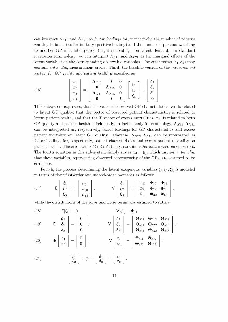
contain, inter alia, measurement errors. Third, the baseline version of the measurement

system for GP quality and patient health is specified as

(16)

x1

x2

x3

x4

=

ΛX11 0 0

0 ΛX22 0

ΛX31 ΛX32 0

0 0 I

ξ1

ξ2

ξ3

+

δ1

δ2

δ3

0

.

This subsystem expresses, that the vector of observed GP characteristics, x1, is related

to latent GP quality, that the vector of observed patient characteristics is related to

latent patient health, and that the T vector of excess mortalities, x3, is related to both

GP quality and patient health. Technically, in factor-analytic terminology, ΛX11,ΛX31

can be interpreted as, respectively, factor loadings for GP characteristics and excess

patient mortality on latent GP quality. Likewise, ΛX22,ΛX32 can be interpreted as

factor loadings for, respectively, patient characteristics and excess patient mortality on

patient health. The error terms (δ1, δ2, δ3) may, contain, inter alia, measurement errors.

The fourth equation in this sub-system simply states x4 = ξ3, which implies, inter alia,

that these variables, representing observed heterogeneity of the GPs, are assumed to be

error-free.

Fourth, the process determining the latent exogenous variables ξ1, ξ2, ξ3 is modeled

in terms of their first-order and second-order moments as follows:

(17) E

ξ1

ξ2

ξ3

=

µξ1

µξ2

µξ3

, V

ξ1

ξ2

ξ3

=

Φ11 Φ12 Φ13

Φ21 Φ22 Φ23

Φ31 Φ32 Φ33

,

while the distributions of the error and noise terms are assumed to satisfy

E[ζ1] = 0, V[ζ1] = Ψ11,(18)

E

δ1

δ2

δ3

=

0

0

0

, V

δ1

δ2

δ3

=

Θδ11 Θδ12 Θδ13

Θδ21 Θδ22 Θδ23

Θδ31 Θδ32 Θδ33

,(19)

E

[ε1

ε2

]=

[0

0

], V

[ε1

ε2

]=

[Θε11 Θε12

Θε21 Θε22

],(20)

[ξ1

ξ2

]⊥ ζ1 ⊥

[δ1

δ2

]⊥

[ε1

ε2

].(21)

11

The final assumption, (21), where ⊥ denotes orthogonal, is crucial for the modeling of

causality and non-causality in Model B. It expresses, inter alia, the assumed exogeneity

for GP quality and patient health. Its essence is that these variables, being modeled by

(17), remain unaffected by the perturbations in the demand equation disturbances, and

the errors in the measurement systems for demand (endogenous) and latent GP quality

and latent patient health (exogenous). Since arguments may be raised that this model

disregards a possible effect of GP quality on the listed patients’ initial health status,

we will in addition consider a modified version, Model C, in which this potential link is

modeled and hence may be tested for.

4 Data

Data sources and data design

Prior to the introduction of the regular GP scheme in June 2001, the health authorities

gathered the information needed to assign GPs to the entire Norwegian population. All

inhabitants were asked to rank their three most preferred GPs in an entry form. The

GPs were asked to report the maximum number of patients they would like to take care

of. The health authorities utilized this information as an input in an algorithm allocating

inhabitants to GPs. Most people got listed with the GP whom they had consulted prior

to the reform (Luras, et al., 2003).

Our data stem from The Norwegian General Practitioners Database supplemented

by a measure of the GP density, as calculated from the number of contracted GPs in

each municipality in June 2001, as well as aggregate age/gender specific mortality rates.

The latter are calculated by means of aggregate mortality rates constructed by Statistics

Norway. The Norwegian General Practitioners Database contains information on all

Norwegian GPs, and the variables describing the individual GPs practice is provided

by the National Insurance Administration (NIA) every six month. The database is

administered by the Norwegian Social Science Data Services, who merge the information

reported by NIA with socio-demographic variables as income, wealth and marital status,

registered by statistics Norway. For GPs practicing in 14 municipalities, sampled by

stratification, the database also includes characteristics for the patients who were listed

in the GP’s practice in June 2001, such as the median income and median wealth, and

the proportion who have not finished high-school. For each GP we know the number

of persons who ranked the GP at the top when returning the entry form, in this paper

to be given the interpretation as an indicator of the demand facing the GP. After the

reform was implemented, the GP database is updated at regular intervals to give the

number of persons who are actually listed in the practice. After excluding observations

with key variables missing, our unbalanced panel data set consists of a sample of 484 GPs

12

observed up to 7 six-month periods.2 The pattern of observation is described in Table 1,

from which we see that 441, or 91 %, of the GPs are observed in all 7 periods.

Table 1: Pattern of observations

Response pattern No. of GPs Freq., % Cum. freq., %

1111111 441 91.12 91.1211111 . . 11 2.27 93.39111111 . 11 2.27 95.661111 . . . 8 1.65 97.31111 . . . . 7 1.45 98.7611 . . . . . 5 1.03 99.7911 . . . 11 1 0.21 100.00

· · 484 100.00 · ·

Table 2 lists and defines the variables applied in this paper, Table 3 gives overall

descriptive statistics for the variables, and Table 4 gives descriptive statistics of the GP-

specific means of the time varying variables. Descriptive statistics for variables at the

level of the municipality are given in Table 5. We distinguish between variables observed

at the GP level and variables which are observed at the municipality level and hence are

common to all GPs practising in the same municipality.

The symbols used for the observable variables in the exposition of Models A and B above,

(x, y, z), have their empirical counterparts among the the variables in Table 2. This cor-

respondence is given below (the GP subscript, for simplicity, suppressed):

Model A:

y′1=[DEMAND], y′2t=[ACTMORTt], x′1 is empty, x′

2t=[EXPMORTt]

z′1=

GPDENS

MARRIEDGP

SPECGEN

SPECCOM

SPECOTHALPHA

IMMIGRGP

FEMALEGP

AGEGP

AGEGPSQ

, z′2=

CENTRAL

LESSCENT

LEASTCENT

LOSUBMIT

LOEDUC

PINCOME

PWEALTH

SPECGEN

SPECCOM

SPECOTH

FEMALEGP

AGEGP

AGEGPSQ

2The GPs from the municipality Tromsø, 44 in total, were excluded from the sample. Here, the regular

GP scheme was implemented already in 1993 and very few inhabitants returned the entry form.

13

Table 2: Variable definitions

Variable Definition, Type of variable Formula

DEAD No. of dead persons on GP’s list

EXPDEAD No. of persons on GP’s list Expected mortality rates based onexpected to die per year age distribution of persons on list and

population age-specific mortality rates

ACTMORT Actual no. of mortalities per 1000 persons listed =DEAD/LISTSIZE

EXPMORT Expected no. of mortalities per 1000 persons listed =EXPDEAD/LISTSIZE

EXCMORT Excess mortality relative to list size =ACTMORT−EXPMORT

LISTSIZE GP’s actual no. of patients

DEMAND No. of persons ranking this GP as mostpreferred when returning entry form

DEMAND1 Demand for this GP normalized againstGP density in municipality =DEMAND * GPDENSITY

AGEGP Age of GP, January 2002

LEAKRATE Share of patients switching to another GP. =no. of persons leaving/LISTSIZE

LOLEAK log(LEAKRATE/(1-LEAKRATE))

FEMALEGP Dummy variable =1 if GP is female

MARRIEDGP Dummy variable =1 if GP is married

IMMIGRGP Dummy variable =1 if GP is non-Scandinavian citizen

SALARY Dummy variable =1 if GP is remunerated bya fixed salary scheme

SPECGEN Dummy variable =1 if GP is a specialist ingeneral practice

SPECCOM Dummy variable =1 if GP is a specialist incommunity medicine

SPECOTH Dummy variable =1 if GP is a specialist inother kind of medicine

LEASTCENT Dummy variable =1 if practice in Least central municipality

LESSCENT Dummy variable =1 if practice in Less central municipality

CENTRAL Dummy variable =1 if practice in Central municipality

MOSTCENT Dummy variable =1 if practice in Most central municipality

PINCOME Median income (NOK1000) ofpersons assigned to this GP in 2001

PWEALTH Median wealth (NOK1000) ofpersons assigned to this GP in 2001

PFORMSUB Share of persons returning forms in 2001among those assigned to this GP in 2001

LOSUBMIT log(PFORMSUB/(1-PFORMSUB))

PEDUC Share of persons without finished high-schoolamong those assigned to this GP in 2001

LOEDUC log(PEDUC/(1-PEDUC))

GPDENSITY No. of GPs per 1000 inhabitans in municipality

14

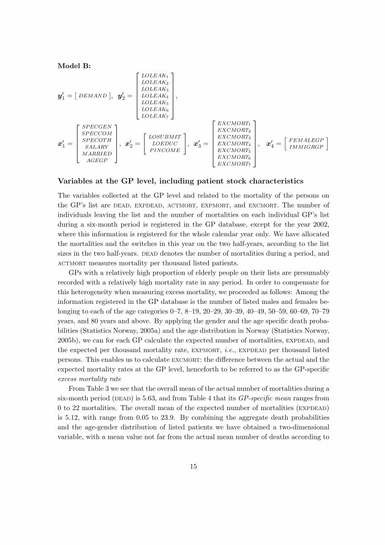
Model B:

y′1 = [ DEMAND ], y′

2 =

LOLEAK1

LOLEAK2

LOLEAK3

LOLEAK4

LOLEAK5

LOLEAK6

LOLEAK7

,

x′1 =

SPECGEN

SPECCOM

SPECOTH

SALARY

MARRIED

AGEGP

, x′

2 =

[LOSUBMIT

LOEDUC

PINCOME

], x′

3 =

EXCMORT1

EXCMORT2

EXCMORT3

EXCMORT4

EXCMORT5

EXCMORT6

EXCMORT7

, x′4 =

[FEMALEGP

IMMIGRGP

]

Variables at the GP level, including patient stock characteristics

The variables collected at the GP level and related to the mortality of the persons on

the GP’s list are DEAD, EXPDEAD, ACTMORT, EXPMORT, and EXCMORT. The number of

individuals leaving the list and the number of mortalities on each individual GP’s list

during a six-month period is registered in the GP database, except for the year 2002,

where this information is registered for the whole calendar year only. We have allocated

the mortalities and the switches in this year on the two half-years, according to the list

sizes in the two half-years. DEAD denotes the number of mortalities during a period, and

ACTMORT measures mortality per thousand listed patients.

GPs with a relatively high proportion of elderly people on their lists are presumably

recorded with a relatively high mortality rate in any period. In order to compensate for

this heterogeneity when measuring excess mortality, we proceeded as follows: Among the

information registered in the GP database is the number of listed males and females be-

longing to each of the age categories 0–7, 8–19, 20–29, 30–39, 40–49, 50–59, 60–69, 70–79

years, and 80 years and above. By applying the gender and the age specific death proba-

bilities (Statistics Norway, 2005a) and the age distribution in Norway (Statistics Norway,

2005b), we can for each GP calculate the expected number of mortalities, EXPDEAD, and

the expected per thousand mortality rate, EXPMORT, i.e., EXPDEAD per thousand listed

persons. This enables us to calculate EXCMORT: the difference between the actual and the

expected mortality rates at the GP level, henceforth to be referred to as the GP-specific

excess mortality rate

From Table 3 we see that the overall mean of the actual number of mortalities during a

six-month period (DEAD) is 5.63, and from Table 4 that its GP-specific mean ranges from

0 to 22 mortalities. The overall mean of the expected number of mortalities (EXPDEAD)

is 5.12, with range from 0.05 to 23.9. By combining the aggregate death probabilities

and the age-gender distribution of listed patients we have obtained a two-dimensional

variable, with a mean value not far from the actual mean number of deaths according to

15

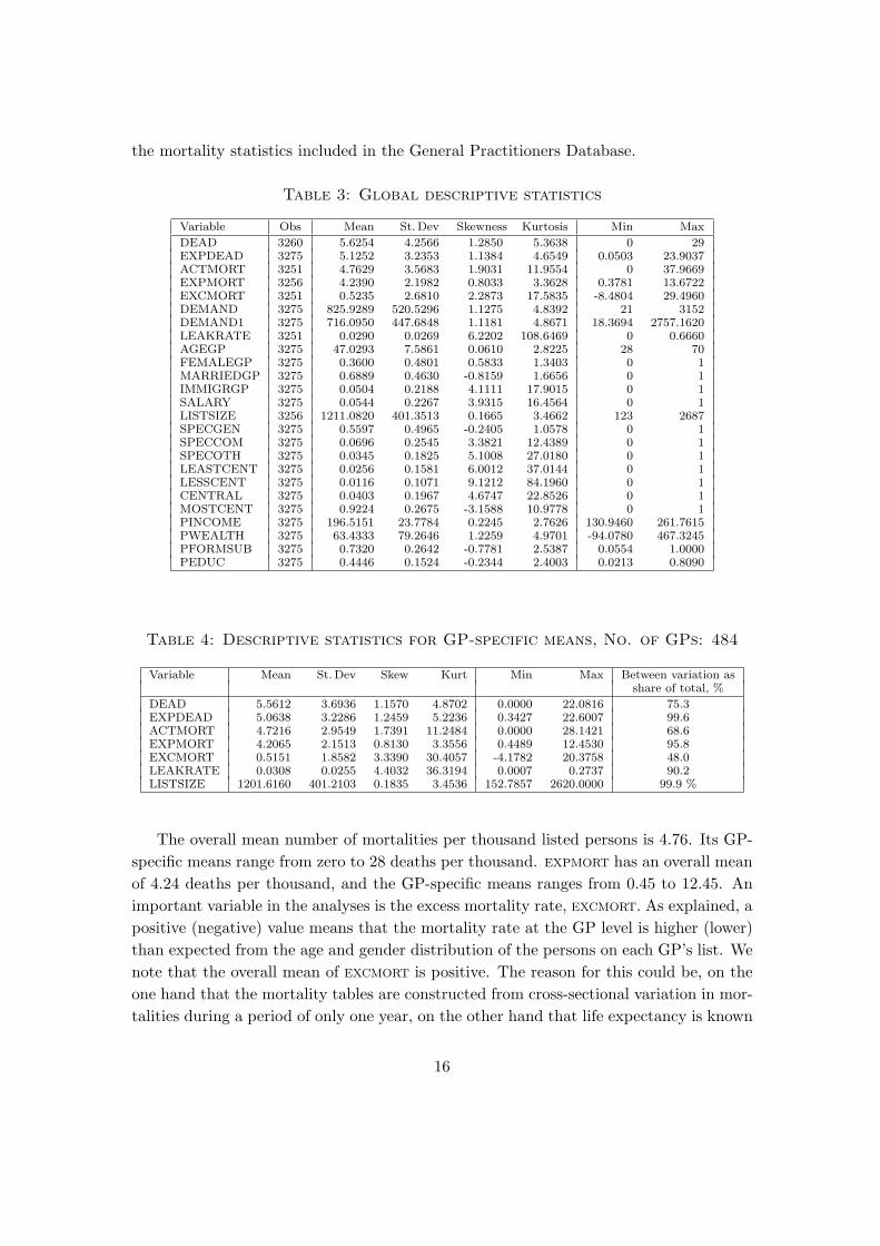
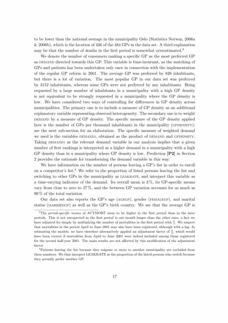
the mortality statistics included in the General Practitioners Database.

Table 3: Global descriptive statistics

Variable Obs Mean St.Dev Skewness Kurtosis Min Max

DEAD 3260 5.6254 4.2566 1.2850 5.3638 0 29EXPDEAD 3275 5.1252 3.2353 1.1384 4.6549 0.0503 23.9037ACTMORT 3251 4.7629 3.5683 1.9031 11.9554 0 37.9669EXPMORT 3256 4.2390 2.1982 0.8033 3.3628 0.3781 13.6722EXCMORT 3251 0.5235 2.6810 2.2873 17.5835 -8.4804 29.4960DEMAND 3275 825.9289 520.5296 1.1275 4.8392 21 3152DEMAND1 3275 716.0950 447.6848 1.1181 4.8671 18.3694 2757.1620LEAKRATE 3251 0.0290 0.0269 6.2202 108.6469 0 0.6660AGEGP 3275 47.0293 7.5861 0.0610 2.8225 28 70FEMALEGP 3275 0.3600 0.4801 0.5833 1.3403 0 1MARRIEDGP 3275 0.6889 0.4630 -0.8159 1.6656 0 1IMMIGRGP 3275 0.0504 0.2188 4.1111 17.9015 0 1SALARY 3275 0.0544 0.2267 3.9315 16.4564 0 1LISTSIZE 3256 1211.0820 401.3513 0.1665 3.4662 123 2687SPECGEN 3275 0.5597 0.4965 -0.2405 1.0578 0 1SPECCOM 3275 0.0696 0.2545 3.3821 12.4389 0 1SPECOTH 3275 0.0345 0.1825 5.1008 27.0180 0 1LEASTCENT 3275 0.0256 0.1581 6.0012 37.0144 0 1LESSCENT 3275 0.0116 0.1071 9.1212 84.1960 0 1CENTRAL 3275 0.0403 0.1967 4.6747 22.8526 0 1MOSTCENT 3275 0.9224 0.2675 -3.1588 10.9778 0 1PINCOME 3275 196.5151 23.7784 0.2245 2.7626 130.9460 261.7615PWEALTH 3275 63.4333 79.2646 1.2259 4.9701 -94.0780 467.3245PFORMSUB 3275 0.7320 0.2642 -0.7781 2.5387 0.0554 1.0000PEDUC 3275 0.4446 0.1524 -0.2344 2.4003 0.0213 0.8090

Table 4: Descriptive statistics for GP-specific means, No. of GPs: 484

Variable Mean St.Dev Skew Kurt Min Max Between variation asshare of total, %

DEAD 5.5612 3.6936 1.1570 4.8702 0.0000 22.0816 75.3EXPDEAD 5.0638 3.2286 1.2459 5.2236 0.3427 22.6007 99.6ACTMORT 4.7216 2.9549 1.7391 11.2484 0.0000 28.1421 68.6EXPMORT 4.2065 2.1513 0.8130 3.3556 0.4489 12.4530 95.8EXCMORT 0.5151 1.8582 3.3390 30.4057 -4.1782 20.3758 48.0LEAKRATE 0.0308 0.0255 4.4032 36.3194 0.0007 0.2737 90.2LISTSIZE 1201.6160 401.2103 0.1835 3.4536 152.7857 2620.0000 99.9 %

The overall mean number of mortalities per thousand listed persons is 4.76. Its GP-

specific means range from zero to 28 deaths per thousand. EXPMORT has an overall mean

of 4.24 deaths per thousand, and the GP-specific means ranges from 0.45 to 12.45. An

important variable in the analyses is the excess mortality rate, EXCMORT. As explained, a

positive (negative) value means that the mortality rate at the GP level is higher (lower)

than expected from the age and gender distribution of the persons on each GP’s list. We

note that the overall mean of EXCMORT is positive. The reason for this could be, on the

one hand that the mortality tables are constructed from cross-sectional variation in mor-

talities during a period of only one year, on the other hand that life expectancy is known

16

to be lower than the national average in the municipality Oslo (Statistics Norway, 2006a

& 2006b), which is the location of 426 of the 484 GPs in the data set. A third explanation

may be that the number of deaths in the first period is somewhat overestimated.3

We denote the number of consumers ranking a specific GP as the most preferred GP

as DEMAND directed towards this GP. This variable is time-invariant, as the matching of

GPs and patients has been undertaken only once in connection with the implementation

of the regular GP reform in 2001. The average GP was preferred by 826 inhabitants,

but there is a lot of variation. The most popular GP in our data set was preferred

by 3152 inhabitants, whereas some GPs were not preferred by any inhabitants. Being

requested by a large number of inhabitants in a municipality with a high GP density

is not equivalent to be strongly requested in a municipality where the GP density is

low. We have considered two ways of controlling for differences in GP density across

municipalities. The primary one is to include a measure of GP density as an additional

explanatory variable representing observed heterogeneity. The secondary one is to weight

DEMAND by a measure of GP density. The specific measure of the GP density applied

here is the number of GPs per thousand inhabitants in the municipality (GPDENSITY);

see the next sub-section for an elaboration. The specific measure of weighted demand

we used is the variables DEMAND1, obtained as the product of DEMAND and GPDENSITY.

Taking DEMAND1 as the relevant demand variable in our analysis implies that a given

number of first rankings is interpreted as a higher demand in a municipality with a high

GP density than in a municipality where GP density is low. Prediction [P2] in Section

2 provides the rationale for transforming the demand variable in this way.

We have information on the number of persons leaving a GP’s list in order to enroll

on a competitor’s list.4 We refer to the proportion of listed persons leaving the list and

switching to other GPs in the municipality as LEAKRATE, and interpret this variable as

a time-varying indicator of the demand. Its overall mean is 3 %, its GP-specific means

vary from close to zero to 27%, and the between GP variation accounts for as much as

90% of the total variation.

Our data set also reports the GP’s age (AGEGP), gender (FEMALEGP), and marital

status (MARRIEDGP) as well as the GP’s birth country. We see that the average GP is

3The period-specific means of ACTMORT seem to be higher in the first period than in the later

periods. This is not unexpected as the first period is one month longer than the other ones, a fact we

have adjusted for simply by multiplying the number of mortalities in the first period with 67. We suspect

that mortalities in the period April to June 2001 may also have been registered, although with a lag. In

estimating the models, we have therefore alternatively applied an adjustment factor of 69, which would

have been correct if mortalities from April to June 2001 were indeed included among those registered

for the second half-year 2001. The main results are not affected by this modification of the adjustment

factor.4Patients leaving the list because they migrate or move to another municipality are excluded from

these numbers. We thus interpret LEAKRATE as the proportion of the listed persons who switch because

they actually prefer another GP.

17

47 years old, that 36 % of the GPs are females and that 69% are married. We have con-

structed a binary variable, IMMIGRGP, equal to 1 if the GP is born in a non-Scandinavian

country. About 5% of the GPs in our sample have this property. The variable denoted

SALARY is a binary variable equal to one if the GP is remunerated by means of a fixed

salary contract when practicing as a GP, and we see that 5 % of the GPs have this kind

of contract.

The number of patients actually listed in the practice at the beginning and end of

each period is registered in the GP database. To take account of within-period changes

of this variable, we construct the average of the numbers recorded at the beginning and

at the end of each period, giving the variable LISTSIZE. Its overall mean is 1211 persons,

while its GP-specific means range from 153 to 2620.

Our data set also reports whether the GP is a specialist in general medicine (dummy

variable SPECGEN), in community medicine (dummy variable SPECCOM) or in another

medical field (dummy variable SPECOTH) – all of which are time-varying dummies, but

the within-GP variation is small. Overall, 56 % of the GPs are specialists in general

medicine, 7% are specialists in community medicine. and 3 % are specialists in an other

field.

Our GP-level data also contain the following information on the patients who were

listed in the practice in June 2001: the median net income and median net wealth among

the listed patients older than 30 years, the proportion of listed patients who are older

than 30 and have not finished high school and the proportion of the listed patients who

submitted the entry form signalling GP preferences. By construction, these variables

are uni-dimensional, as this information is not updated after the implementation of the

regular General Practitioner Scheme. The income and wealth variables, measured in

1.000 NOK, PINCOME and PWEALTH, have overall means 196.5 and 63.4, respectively.

Not unexpectedly, they vary considerably: the GP whose listed patients are on average

richest, have a median income twice that of the GP whose listed patients have the lowest

median income. The corresponding median wealth, PWEALTH extends from −94.2 to

467.3. In the LISREL analysis, after some trial runs, we decided to exclude PWEALTH

from the variable list, in order to ensure convergence. We suspect that the reason for

this is that income and wealth are highly correlated.

Finally, PFORMSUB denotes the proportion of the listed patients who submitted the

entry form prior to the implementation of the regular General Practitioner Scheme. This

variable varies from nearly zero to one, indicating that some GPs were not assigned any

patients who submitted the entry form, while other GPs were assigned only patients who

submitted the form. The mean of this variable is 0.73, indicating that the average GP

have a list where 73% of the patients submitted the entry form. We denote by PEDUC

the proportion of the listed patients who are older than 30 and have not finished high

school. We see that the average GP have 45 % of the listed patients characterized by not

having finished high school. This share also varies considerably, from 2% to 81 %.

18

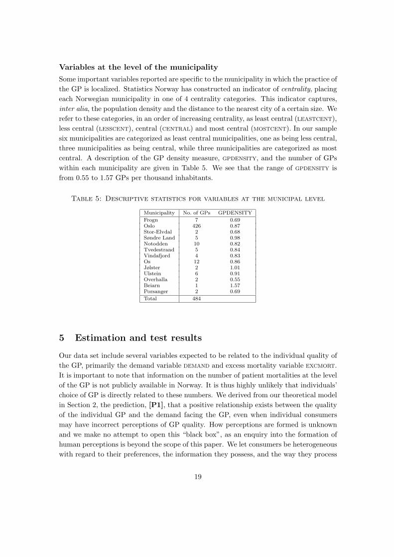
Variables at the level of the municipality

Some important variables reported are specific to the municipality in which the practice of

the GP is localized. Statistics Norway has constructed an indicator of centrality, placing

each Norwegian municipality in one of 4 centrality categories. This indicator captures,

inter alia, the population density and the distance to the nearest city of a certain size. We

refer to these categories, in an order of increasing centrality, as least central (LEASTCENT),

less central (LESSCENT), central (CENTRAL) and most central (MOSTCENT). In our sample

six municipalities are categorized as least central municipalities, one as being less central,

three municipalities as being central, while three municipalities are categorized as most

central. A description of the GP density measure, GPDENSITY, and the number of GPs

within each municipality are given in Table 5. We see that the range of GPDENSITY is

from 0.55 to 1.57 GPs per thousand inhabitants.

Table 5: Descriptive statistics for variables at the municipal level

Municipality No. of GPs GPDENSITY

Frogn 7 0.69Oslo 426 0.87Stor-Elvdal 2 0.68Søndre Land 5 0.98Notodden 10 0.82Tvedestrand 5 0.84Vindafjord 4 0.83Os 12 0.86Jølster 2 1.01Ulstein 6 0.91Overhalla 2 0.55Beiarn 1 1.57Porsanger 2 0.69

Total 484

5 Estimation and test results

Our data set include several variables expected to be related to the individual quality of

the GP, primarily the demand variable DEMAND and excess mortality variable EXCMORT.

It is important to note that information on the number of patient mortalities at the level

of the GP is not publicly available in Norway. It is thus highly unlikely that individuals’

choice of GP is directly related to these numbers. We derived from our theoretical model

in Section 2, the prediction, [P1], that a positive relationship exists between the quality

of the individual GP and the demand facing the GP, even when individual consumers

may have incorrect perceptions of GP quality. How perceptions are formed is unknown

and we make no attempt to open this “black box”, as an enquiry into the formation of

human perceptions is beyond the scope of this paper. We let consumers be heterogeneous

with regard to their preferences, the information they possess, and the way they process

19

information. Consumers may choose the same GP for different reasons, or different GPs

for the same reason. We expect however that the GPs’ appearance, experiences from

earlier consultations with available GPs, advice from relatives and friends and even rumor

to enter the “black box” as inputs in the formation of individuals’ quality perceptions.

As explained in Sections 3 and 4, the statistical modeling of the ‘causality chain’ giving

rise to this relationship is rather different in the two econometric models we consider,

Model A and Model B. In addition, mainly as a robustness check of our main conclusion,

results obtained from a third model, Model C – essentially a modification of Model B in

one important respect – will be briefly considered at the end.

The estimation procedure for Model A, Version 2, represented by Equation (12),

is, as explained in Section 3, a stepwise procedure. Using in both steps modules in the

STATA 9 software, we estimate in the first step the effect of the variables representing

observed heterogeneity and other assumed exogenous variables on the mortality rates and

extract the predicted value of the random effect for each GP in the sample, ALPHAHAT.5

In estimating this mortality equation, i.e., the second equation of (12), we allow for the

possibility that the residuals are not independent within municipalities, and report robust

standard errors. In the second step, this prediction, treated as an exogenous variable, is

inserted in the demand equation, i.e., the first equation of (12). 6

For the multi-equation model, Model B, we apply the Maximum Likelihood (ML)

procedure in the LISREL 8.80 software. 7 The actual number of linear equations to be

simultaneously estimated is 25. In this model both the quality of the individual GPs and

the unobserved aggregate health status of the listed patients occur as latent exogenous

variables, as explained in Section 3.

Results for Model A

The mortality equation

The dependent variable in this equation is ACTMORT. Observable heterogeneity is con-

trolled for in various ways. First, to control for differences in the age and gender dis-

tribution of the GPs’ listed patients, we include the expected mortality rates EXPMORT

as an explanatory variable. Second, to account for heterogeneity between municipali-

5See Hsiao (2003, Section 6.2.2.c) and Lee and Griffiths (1979) on the prediction of random effects

from panel data.6An even simpler alternative also considered is a single-equation model where the excess mortality

rate is inserted directly as a quality indicator in the demand equation – in a sense merging the two

equations in (12) into one equation. The underlying assumption is that the GP specific level of patient

excess mortality is exogenous. This approach, however, is defective to the extent that the GPs have an

inhomogeneous patient stock with respect to the average health status, which will induce a bias in the

coefficient estimate of the quality variable. The results from this ‘single-equation version’ of Model A is

presented in Appendix A, Table A.17The Covariances and Means to be analyzed are estimated by the EM procedure, as there are some

missing observations due to the unbalanced panel data.

20

ties of different centrality, we include the centrality dummies LEASTCENT, LESSCENT and

CENTRAL. Third, to account for observable GP heterogeneity we include AGEGP, three

GP speciality dummies as well as FEMALEGP. Fourth, we include variables describing the

listed patients, with intention to control for the possibility that the average health status

of patients varies between GPs. Since there is evidence in the medical literature that

life expectancy and health status is related to education, income and wealth (Lantz et

al., 1998, Papas et al., 1993), we include PEDUC, PINCOME and PWEALTH as proxies for the

average health status of the persons listed with each GP. Fifth, as discussed in Section 2,

still another kind of heterogeneity may also occur: individuals who chose not to submit

the entry form stating their preferences for certain GPs, may have an average health

status different from those who returned the entry form. We take account of this by in-

cluding PFORMSUB as an explanatory variable. Since the range of PEDUC and PFORMSUB

is restricted to the (0, 1) interval, we transform them by the log-odds using the formula

ln( x1−x

) in order to extend their range to (−∞,+∞) which gives a better balance with

the unbounded range of the other explanatory variables.

Table 6: Model A. Mortality equation, GLS estimates

No. of obs.=3251. No. of GPs=484. Obs. per GP.: min=1, mean=6.7, max=7

Regressor Estimate Std.Err.

EXPMORT 1.2900 0.0383**CENTRAL -0.6365 0.1656**LESSCENT -0.3897 0.0434**LEASTCENT -0.2359 0.2578LOSUBMIT -0.0496 0.0025**LOEDUC -0.0468 0.0185*PINCOME -0.0097 0.0015**PWEALTH -0.0094 0.0006**SPECGEN 0.0156 0.0323SPECCOM 0.2164 0.0536**SPECOTH -0.6432 0.0717**FEMALEGP -0.1720 0.0422**AGEGP -0.0547 0.0498AGEGPSQ 0.0003 0.0005CONST 4.0038 1.0395*

σα2 1.3602σu2 2.1076ρ 0.2940

R2

within 0.0578between 0.7104overall 0.5071

Wald chi2(11) 165868p-value 0.0000

∗) Significantly 6= 0 at the 5% level (two-tailed test)

∗∗) Significantly 6= 0 at the 1% level (two-tailed test)

The results from the mortality equation are presented in Table 6. All of the es-

timated coefficients except LEASTCENT, SPECGEN, AGEGP and AGEGPSQ are statistically

significant, and the overall R2 is rather high: 0.5071. The coefficient of EXPMORT is pos-

21

itive, as expected, since high expected mortality should have a positive effect on actual

mortality. Further, GPs having their practice in a central or less central municipality

have a significantly lower patient mortality rate than GPs in most central municipalities.

The negative estimated coefficient of LOSUBMIT indicates that GPs who were assigned

a high proportion of the persons who expressed their GP preferences in advance, have

lower patient mortality than GPs who obtained a low proportion of patients who actively

selected their GP. The coefficient on the education variable is negative, which is not in ac-

cordance with intuition saying that GPs with a high proportion of low-educated patients

have a higher mortality rate and may be attributed to education being correlated with

income and wealth.8 The estimated coefficients of income and wealth have the expected

negative signs. Since these variables are measured in 1000 NOK, an increase in PINCOME

and PWEALTH of NOK 100.000 would be accompanied by a reduction in the mortality

rates of 0.97 and 0.94 deaths per thousand, respectively. We see that, ceteris paribus, the

patient mortality rate of GPs who are specialists in community medicine is significantly

higher and that of GPs who are specialists in a field other than general medicine and

community medicine is significantly lower than the patient mortality rate of other GPs.

Finally, female GPs have, ceteris paribus, a lower mortality rate of their patient stock

than male GPs.

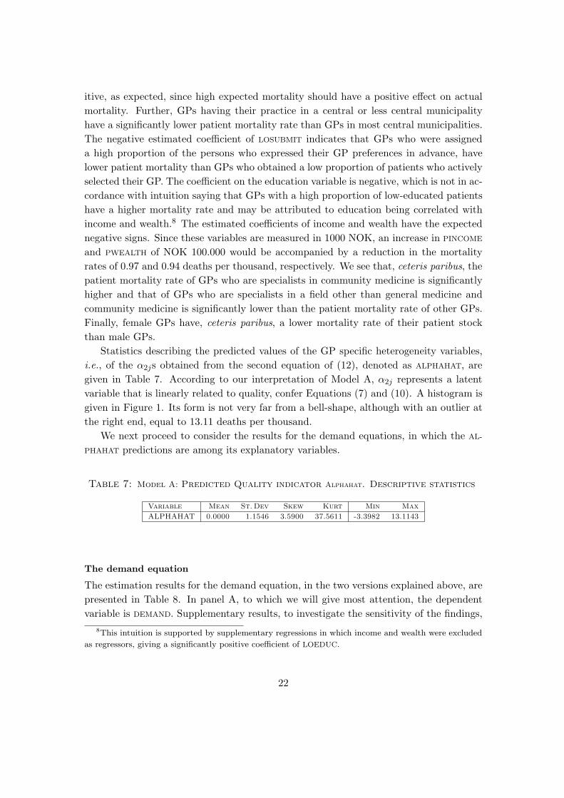
Statistics describing the predicted values of the GP specific heterogeneity variables,

i.e., of the α2js obtained from the second equation of (12), denoted as ALPHAHAT, are

given in Table 7. According to our interpretation of Model A, α2j represents a latent

variable that is linearly related to quality, confer Equations (7) and (10). A histogram is

given in Figure 1. Its form is not very far from a bell-shape, although with an outlier at

the right end, equal to 13.11 deaths per thousand.

We next proceed to consider the results for the demand equations, in which the AL-

PHAHAT predictions are among its explanatory variables.

Table 7: Model A: Predicted Quality indicator Alphahat. Descriptive statistics

Variable Mean St.Dev Skew Kurt Min Max

ALPHAHAT 0.0000 1.1546 3.5900 37.5611 -3.3982 13.1143

The demand equation

The estimation results for the demand equation, in the two versions explained above, are

presented in Table 8. In panel A, to which we will give most attention, the dependent

variable is DEMAND. Supplementary results, to investigate the sensitivity of the findings,

8This intuition is supported by supplementary regressions in which income and wealth were excluded

as regressors, giving a significantly positive coefficient of LOEDUC.

22

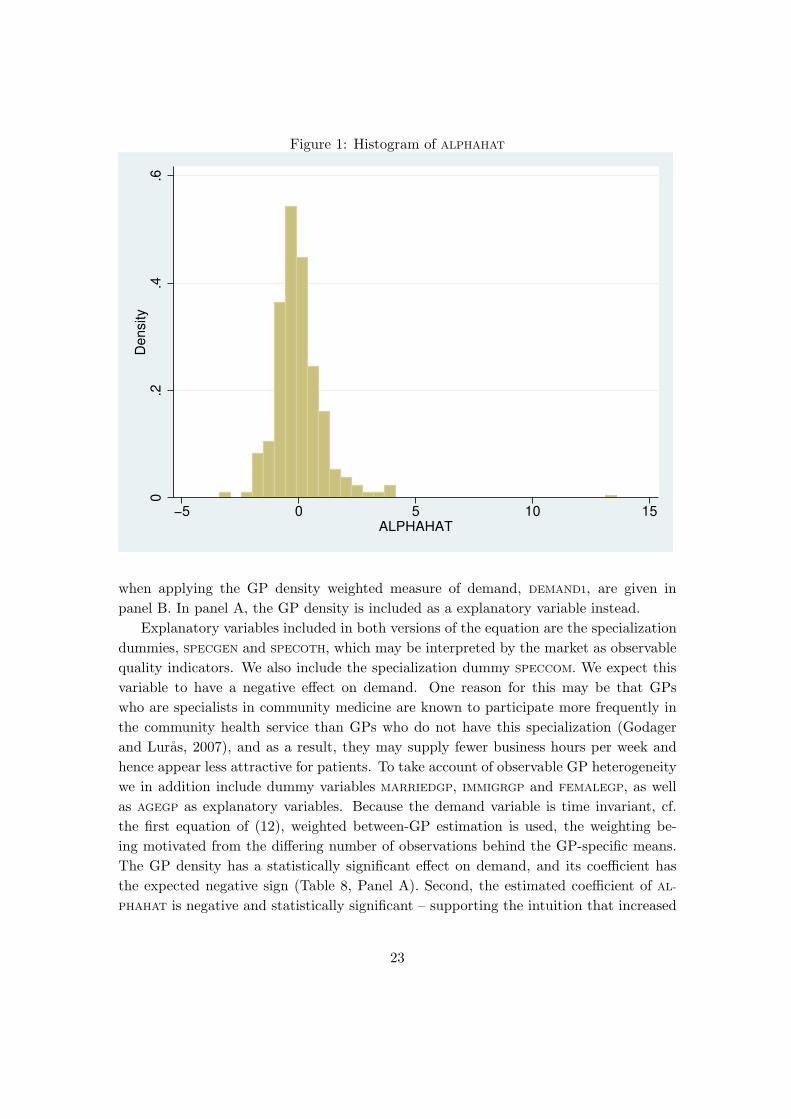
Figure 1: Histogram of ALPHAHAT0

.2.4

.6D

en

sity

−5 0 5 10 15ALPHAHAT

when applying the GP density weighted measure of demand, DEMAND1, are given in

panel B. In panel A, the GP density is included as a explanatory variable instead.

Explanatory variables included in both versions of the equation are the specialization

dummies, SPECGEN and SPECOTH, which may be interpreted by the market as observable

quality indicators. We also include the specialization dummy SPECCOM. We expect this

variable to have a negative effect on demand. One reason for this may be that GPs

who are specialists in community medicine are known to participate more frequently in

the community health service than GPs who do not have this specialization (Godager

and Luras, 2007), and as a result, they may supply fewer business hours per week and

hence appear less attractive for patients. To take account of observable GP heterogeneity

we in addition include dummy variables MARRIEDGP, IMMIGRGP and FEMALEGP, as well

as AGEGP as explanatory variables. Because the demand variable is time invariant, cf.

the first equation of (12), weighted between-GP estimation is used, the weighting be-

ing motivated from the differing number of observations behind the GP-specific means.

The GP density has a statistically significant effect on demand, and its coefficient has

the expected negative sign (Table 8, Panel A). Second, the estimated coefficient of AL-

PHAHAT is negative and statistically significant – supporting the intuition that increased

23

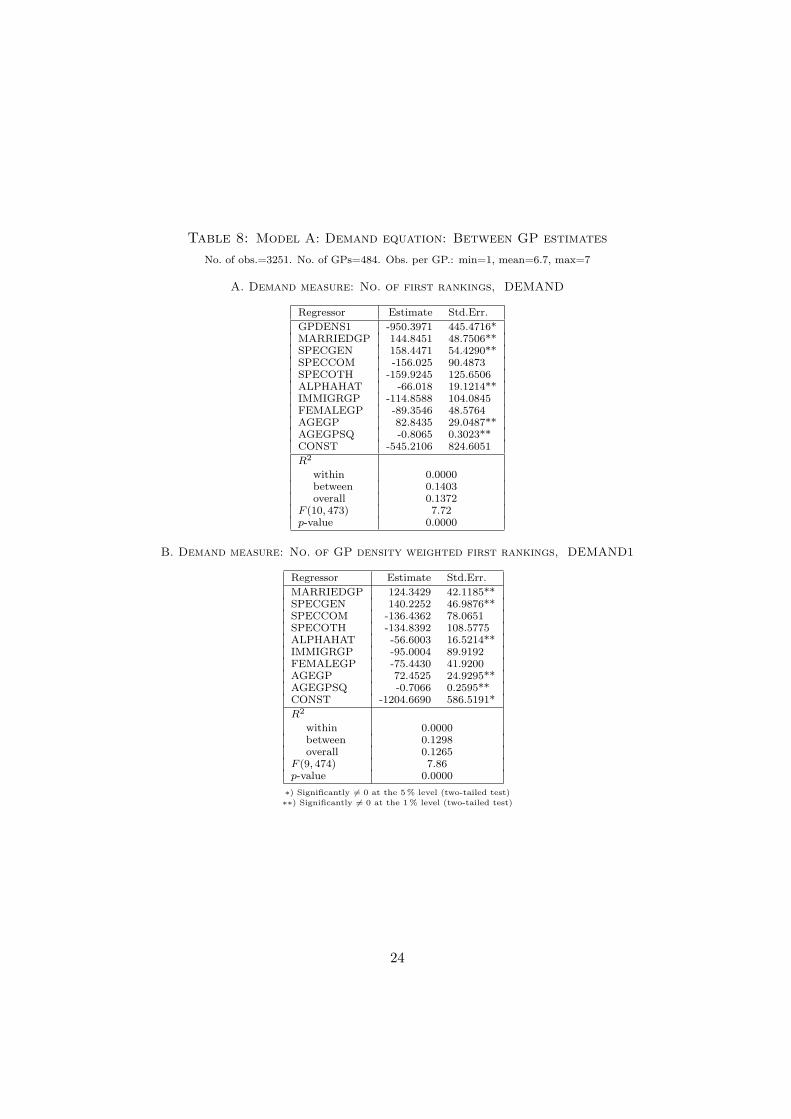
Table 8: Model A: Demand equation: Between GP estimates

No. of obs.=3251. No. of GPs=484. Obs. per GP.: min=1, mean=6.7, max=7

A. Demand measure: No. of first rankings, DEMAND

Regressor Estimate Std.Err.

GPDENS1 -950.3971 445.4716*MARRIEDGP 144.8451 48.7506**SPECGEN 158.4471 54.4290**SPECCOM -156.025 90.4873SPECOTH -159.9245 125.6506ALPHAHAT -66.018 19.1214**IMMIGRGP -114.8588 104.0845FEMALEGP -89.3546 48.5764AGEGP 82.8435 29.0487**AGEGPSQ -0.8065 0.3023**CONST -545.2106 824.6051

R2

within 0.0000between 0.1403overall 0.1372

F (10, 473) 7.72p-value 0.0000

B. Demand measure: No. of GP density weighted first rankings, DEMAND1

Regressor Estimate Std.Err.

MARRIEDGP 124.3429 42.1185**SPECGEN 140.2252 46.9876**SPECCOM -136.4362 78.0651SPECOTH -134.8392 108.5775ALPHAHAT -56.6003 16.5214**IMMIGRGP -95.0004 89.9192FEMALEGP -75.4430 41.9200AGEGP 72.4525 24.9295**AGEGPSQ -0.7066 0.2595**CONST -1204.6690 586.5191*

R2

within 0.0000between 0.1298overall 0.1265

F (9, 474) 7.86p-value 0.0000

∗) Significantly 6= 0 at the 5% level (two-tailed test)

∗∗) Significantly 6= 0 at the 1% level (two-tailed test)

24

quality induces increased demand facing the GP. Furthermore, the estimated effect of

MARRIEDGP and SPECGEN indicate that being married and being a specialist in general

medicine contribute, ceteris paribus, to a higher market demand. While FEMALEGP is

not statistically significant, AGEGP comes out with a positive and statistically significant

effect. The latter results may be explained by the fact that a GP’s age is correlated

with the number of years in GP practice, and that a GP who has been practicing for a

long time may be included in the choice set of a larger proportion of the consumers in

the market. This mechanism, however, is not explicitly accounted for in our theoretical

model. It would have been possible to capture it by introducing heterogeneous groups

of consumers with different choice sets within the same market, and this can be done

simply by furnishing the parameter N with a group subscript.

As to the signs of the effects as well as their significance, the results in Panel B are

very similar to those in Panel A. Being married and being a specialist in general medicine

are both estimated to have a positive effect according to this model as well, and again,

AGEGP comes out with a significantly positive coefficient.

Results for Model B

The path diagram produced by the LISREL program, given in Figure 2, is a useful

starting point for the description of the approach. As explained in Section 3, the LISREL

model consists of two parts: the measurement equations and the structural equations,

representing the relationship between the latent variables. In the sequel, we will follow

the conventional LISREL notation, letting latent variables be indicated by names having

capitalized first letter, whereas observable variables are written without capitalized first

letters.9 The measurement model specifies how our unobserved, latent variables Quality,

Health and Demand are indicated by observed variables; cf. equations (16) and (15).

By modeling the demand facing the individual GP as a latent variable we are able

to utilize information on the rate at which patients leave the GP’s list in order to join a

competitor’s list. This approach thus takes into account how the demand facing the GPs

has developed after the introduction of the General Practitioner Scheme. In our case the

measurement model consists of two parts. The measurement equations for the exogenous

latent variables, in the LISREL notation in Section 3 referred to as ξ-variables, are

henceforth referred to as the X-measurement model. The measurement equations for the

dependent latent variable, in LISREL notation referred to as an η-variable, is henceforth

referred to as the Y -measurement model. When interpreting the approach and the results

below, it should be recalled that the panel structure of the data – including the repeated

observations of patients leaving the GP’s list as well as of the excess mortality rates at

the level of the GP – is essential for obtaining the inference we want to make, as the

three latent variables in focus on Model B, Quality, Health and Demand, are all time

9We denote the variables Femalegp and Immigrant as if they were latent. See note 1.

25

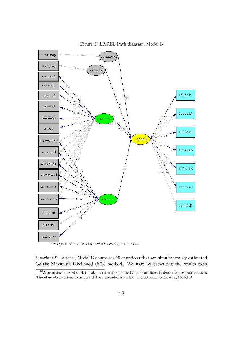
Figure 2: LISREL Path diagram, Model B

invariant.10 In total, Model B comprises 25 equations that are simultaneously estimated

by the Maximum Likelihood (ML) method. We start by presenting the results from

10As explained in Section 4, the observations from period 2 and 3 are linearly dependent by construction.

Therefore observations from period 2 are excluded from the data set when estimating Model B.

26

estimation of the structural equation before presenting the results from the estimation

of the equations in the two measurement models.

The structural model (demand equation)

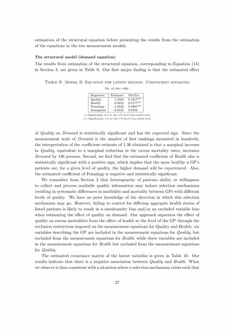
The results from estimation of the structural equation, corresponding to Equation (14)

in Section 3, are given in Table 9. Our first major finding is that the estimated effect

Table 9: Model B: Equation for latent demand. Coefficient estimates

No. of obs.=484.

Regressor Estimate Std.Err.

Quality 1.3583 0.1617**Health 0.0456 0.0177**Femalegp -1.0422 0.3881**Immigrant -0.9545 0.8356

∗) Significantly 6= 0 at the 5% level (two-tailed test)

∗∗) Significantly 6= 0 at the 1% level (two-tailed test)

of Quality on Demand is statistically significant and has the expected sign. Since the

measurement scale of Demand is the number of first rankings measured in hundreds,

the interpretation of the coefficient estimate of 1.36 obtained is that a marginal increase

in Quality, equivalent to a marginal reduction in the excess mortality rates, increases

Demand by 136 persons. Second, we find that the estimated coefficient of Health also is

statistically significant with a positive sign, which implies that the more healthy a GP’s

patients are, for a given level of quality, the higher demand will be experienced. Also,

the estimated coefficient of Femalegp is negative and statistically significant.

We remember from Section 2 that heterogeneity of patients ability or willingness

to collect and process available quality information may induce selection mechanisms

resulting in systematic differences in morbidity and mortality between GPs with different

levels of quality. We have no prior knowledge of the direction in which this selection

mechanism may go. However, failing to control for differing aggregate health status of

listed patients is likely to result in a simultaneity bias and/or an excluded variable bias

when estimating the effect of quality on demand. Our approach separates the effect of

quality on excess mortalities from the effect of health at the level of the GP through the

exclusion restrictions imposed on the measurement equations for Quality and Health: six

variables describing the GP are included in the measurement equations for Quality, but

excluded from the measurement equations for Health, while three variables are included

in the measurement equations for Health but excluded from the measurement equations

for Quality.

The estimated covariance matrix of the latent variables is given in Table 10. Our

results indicate that there is a negative association between Quality and Health. What

we observe is thus consistent with a situation where a selection mechanism exists such that

27

Table 10: Model B: Variance and correlation matrix of latent variables

Variances along the main diagonal, correlation coefficients below the diagonal. No. of obs.=484.

Demand Quality Health

Demand 15.6585Quality 0.4358 2.4438Health 0.0123 -0.4064 460.2335

GPs with low quality of services are endowed with a patient stock with a better health,

as compared to GPs with higher quality of services. One may argue that Model B does

not reveal the effect of the GPs’ quality on the initial health state of listed patients, as

it is set up to measure the effect of quality when controlling for initial health status of

patients showing between GP variation. To address the latter issue, and for the purpose

of conducting a robustness check of our main findings, we have additionally estimated

an alternative LISREL model where all latent variables enter as η variables, i.e., as

formally endogenous – Quality and Health being exogenous latent variables in Model B.

Such a model setup allows the estimation of the marginal effect of GP’s quality on the

initial state of health. The results from this model, denoted as Model C, are reported in

Appendix A. The results confirm the results from Model B, that latent quality affects

latent demand positively. The numerical size of the effect is somewhat smaller, however.

The most important single result from estimation of Model C is that quality is found not

to have significant effect on the aggregate health status of the GP’s listed patients.

The X-measurement model

The left hand side of Figure 2 describes the relations in the X-measurement model.

Arrows indicate the relation between the observable variables and the ξ variables, and

the reported numbers on each arrow corresponds to the estimated or fixed ’factor load-

ing‘.Since latent variables by definition do not have a scale of measurement, the scale of

the latent variables are defined by fixing one or more of the factor loadings. In order

to make the results from LISREL estimation comparable to the results of the previous

model we have scaled the ξ variable Quality to be measured in (negative) units of per

thousand excess mortality rates. By fixing the factor loading of pincome on Health, we

have scaled the ξ variable Health to be measured in units of thousand Norwegian kro-

ner. Note that the arrows representing the fixed factor loadings are shaded compared

to the massive arrows representing estimated factor loadings. Although formally treated

as latent variables, the ξ-variables Femalegp and Immigrgp are identical to their observ-

able counterparts femalegp and immigrgp. This is done by fixing the factor loadings to

unity and fixing the error terms in the two corresponding regression equations to zero.

The interpretation is that the GP’s gender and country of birth is expected to affect

the demand directly, without being indicators of either quality or health status of listed

28

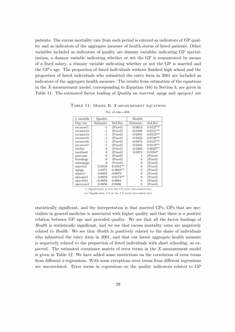
patients. The excess mortality rate from each period is entered as indicators of GP qual-

ity and as indicators of the aggregate measure of health status of listed patients. Other

variables included as indicators of quality are dummy variables indicating GP special-

ization, a dummy variable indicating whether or not the GP is remunerated by means

of a fixed salary, a dummy variable indicating whether or not the GP is married and

the GP’s age. The proportion of listed individuals without finished high school and the

proportion of listed individuals who submitted the entry form in 2001 are included as

indicators of the aggregate health measure. The results from estimation of the equations

in the X-measurement model, corresponding to Equation (16) in Section 3, are given in

Table 11. The estimated factor loading of Quality on married, agegp and specgen1 are

Table 11: Model B: X-measurement equations

No. of obs.=484.

ξ variable Quality Health

Dep var Estimate Std.Err. Estimate Std.Err.

excmort1 -1 (Fixed) -0.0614 0.0127**excmort3 -1 (Fixed) -0.0498 0.0121**excmort4 -1 (Fixed) -0.0581 0.0123**excmort5 -1 (Fixed) -0.0458 0.0120**excmort6 -1 (Fixed) -0.0673 0.0127**excmort7 -1 (Fixed) -0.0445 0.0119**loeduc 0 (Fixed) -0.0283 0.0025**losubmit 0 (Fixed) 0.0374 0.0158*pincome 0 (Fixed) 1 (Fixed)femalegp 0 (Fixed) 0 (Fixed)immigrgp 0 (Fixed) 0 (Fixed)married 0.0558 0.0161** 0 (Fixed)agegp 1.0471 0.2692** 0 (Fixed)salary1 0.0033 0.0079 0 (Fixed)specgen1 0.0658 0.0174** 0 (Fixed)specoth1 -0.0056 0.0064 0 (Fixed)speccom1 0.0056 0.0086 0 (Fixed)

∗) Significantly 6= 0 at the 5% level (two-tailed test)

∗∗) Significantly 6= 0 at the 1% level (two-tailed test)

statistically significant, and the interpretation is that married GPs, GPs that are spe-

cialists in general medicine is associated with higher quality and that there is a positive

relation between GP age and provided quality. We see that all the factor loadings of

Health is statistically significant, and we see that excess mortality rates are negatively

related to Health. We see that Health is positively related to the share of individuals

who submitted the entry form in 2001, and that our latent aggregate health measure

is negatively related to the proportion of listed individuals with short schooling, as ex-

pected. The estimated covariance matrix of error terms in the X-measurement model

is given in Table 12. We have added some restrictions on the correlation of error terms

from different x-regressions. With some exceptions error terms from different regressions

are uncorrelated. Error terms in regressions on the quality indicators related to GP

29

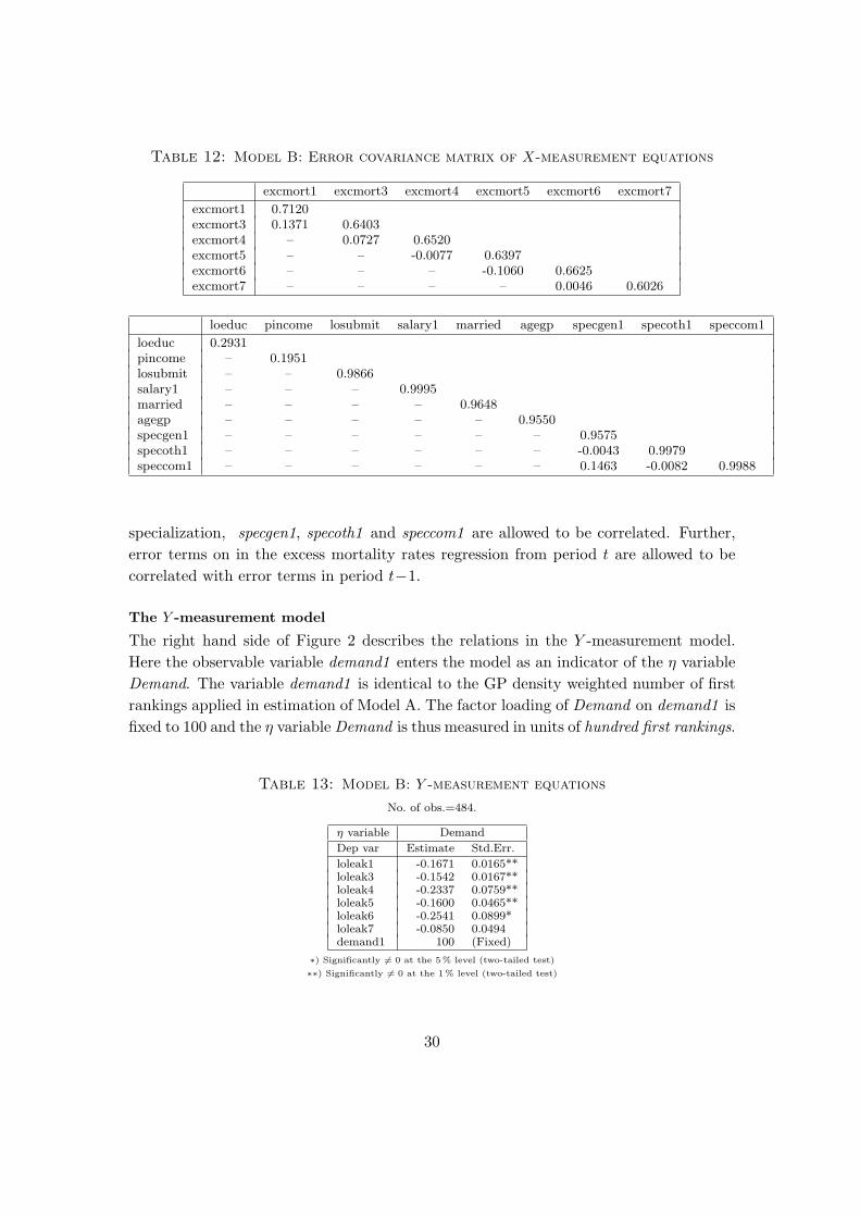
Table 12: Model B: Error covariance matrix of X-measurement equations

excmort1 excmort3 excmort4 excmort5 excmort6 excmort7

excmort1 0.7120excmort3 0.1371 0.6403excmort4 – 0.0727 0.6520excmort5 – – -0.0077 0.6397excmort6 – – – -0.1060 0.6625excmort7 – – – – 0.0046 0.6026

loeduc pincome losubmit salary1 married agegp specgen1 specoth1 speccom1

loeduc 0.2931pincome – 0.1951losubmit – – 0.9866salary1 – – – 0.9995married – – – – 0.9648agegp – – – – – 0.9550specgen1 – – – – – – 0.9575specoth1 – – – – – – -0.0043 0.9979speccom1 – – – – – – 0.1463 -0.0082 0.9988

specialization, specgen1, specoth1 and speccom1 are allowed to be correlated. Further,

error terms on in the excess mortality rates regression from period t are allowed to be

correlated with error terms in period t−1.

The Y -measurement model

The right hand side of Figure 2 describes the relations in the Y -measurement model.

Here the observable variable demand1 enters the model as an indicator of the η variable

Demand. The variable demand1 is identical to the GP density weighted number of first

rankings applied in estimation of Model A. The factor loading of Demand on demand1 is

fixed to 100 and the η variable Demand is thus measured in units of hundred first rankings.

Table 13: Model B: Y -measurement equations

No. of obs.=484.

η variable Demand

Dep var Estimate Std.Err.

loleak1 -0.1671 0.0165**loleak3 -0.1542 0.0167**loleak4 -0.2337 0.0759**loleak5 -0.1600 0.0465**loleak6 -0.2541 0.0899*loleak7 -0.0850 0.0494demand1 100 (Fixed)

∗) Significantly 6= 0 at the 5% level (two-tailed test)

∗∗) Significantly 6= 0 at the 1% level (two-tailed test)

30

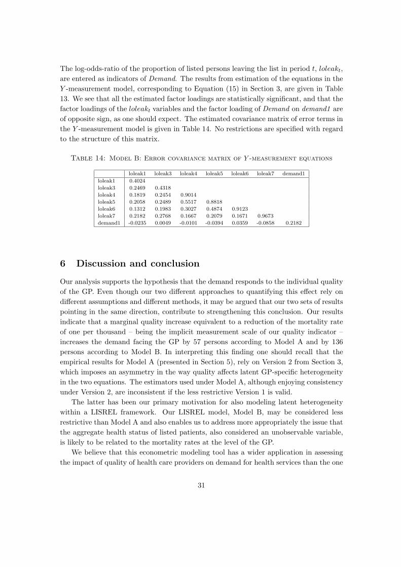
The log-odds-ratio of the proportion of listed persons leaving the list in period t, loleakt,

are entered as indicators of Demand. The results from estimation of the equations in the

Y -measurement model, corresponding to Equation (15) in Section 3, are given in Table

13. We see that all the estimated factor loadings are statistically significant, and that the

factor loadings of the loleakt variables and the factor loading of Demand on demand1 are

of opposite sign, as one should expect. The estimated covariance matrix of error terms in

the Y -measurement model is given in Table 14. No restrictions are specified with regard

to the structure of this matrix.

Table 14: Model B: Error covariance matrix of Y -measurement equations

loleak1 loleak3 loleak4 loleak5 loleak6 loleak7 demand1

loleak1 0.4024

loleak3 0.2469 0.4318

loleak4 0.1819 0.2454 0.9014

loleak5 0.2058 0.2489 0.5517 0.8818

loleak6 0.1312 0.1983 0.3027 0.4874 0.9123

loleak7 0.2182 0.2768 0.1667 0.2079 0.1671 0.9673

demand1 -0.0235 0.0049 -0.0101 -0.0394 0.0359 -0.0858 0.2182

6 Discussion and conclusion

Our analysis supports the hypothesis that the demand responds to the individual quality

of the GP. Even though our two different approaches to quantifying this effect rely on

different assumptions and different methods, it may be argued that our two sets of results

pointing in the same direction, contribute to strengthening this conclusion. Our results

indicate that a marginal quality increase equivalent to a reduction of the mortality rate

of one per thousand – being the implicit measurement scale of our quality indicator –

increases the demand facing the GP by 57 persons according to Model A and by 136

persons according to Model B. In interpreting this finding one should recall that the

empirical results for Model A (presented in Section 5), rely on Version 2 from Section 3,

which imposes an asymmetry in the way quality affects latent GP-specific heterogeneity

in the two equations. The estimators used under Model A, although enjoying consistency

under Version 2, are inconsistent if the less restrictive Version 1 is valid.

The latter has been our primary motivation for also modeling latent heterogeneity

within a LISREL framework. Our LISREL model, Model B, may be considered less

restrictive than Model A and also enables us to address more appropriately the issue that

the aggregate health status of listed patients, also considered an unobservable variable,

is likely to be related to the mortality rates at the level of the GP.

We believe that this econometric modeling tool has a wider application in assessing

the impact of quality of health care providers on demand for health services than the one

31

presented here. Our LISREL model separates the effect of quality on outcome measures

from the effect of patient health at the provider level through the exclusion restrictions

imposed on the measurement equations for the latent variables Quality and Health. An

idea for future research is to apply this modelling and estimation strategy to matched

hospital-patient data, in order to measure the impact of hospital quality on demand.

An important question from the point of view of policy implications is: how strong is

the effect of quality on demand? In the context of regression models answers to such

questions are often provided by means of appropriate elasticities. Due to the fact that the

mean value of latent variables are undefined, the elasticities of interest, such as Quality

elasticity of demand are also undefined. However, to get a ‘metric’ for assessing the

magnitude of the effect we may compare the effect of quality on demand with the effect

of the observable GP specific variables like the GP gender dummy and the dummy for

whether or not the GP is born in a non-scandinavian country. In case of model B, this

can be achieved by utilizing the standardized solution of our LISREL estimation in which

all effects are scaled in terms of their standard deviation. The standardized solution thus

obtained indicates that the effect of quality on demand is more than four times the effect

of the GP gender dummy and ten times the effect of non-Scandinavian GP dummy. It

is also illuminating to interpret the latter effect in relation to the standard deviation

of the Quality variable σQ (confer Table 10). We then find that an increase in quality

equivalent to a reduction of the patient mortality rate by one per thousand corresponds

to a change in Quality equal to 0.6397σQ. An increase of this order of magnitude results

in an increase in Demand corresponding to 16% relative to the global mean of DEMAND,

given in table Table 3.

References

Arrow, K.E. 1963. Uncertainty and the welfare economics of medical care. American Economic Review53, 941-973.

Aigner, D.J., Hsiao, C., Kapteyn, A., and Wansbeek, T. (1984): Latent Variable Models in Economet-rics, in Griliches, Z. and M.D. Intriligator (eds.): Handbook of econometrics, vol. II, Amsterdam:North-Holland, 1321-1393.

Burns, L.R. and Wholey, D.R. (1992): The Impact of Physician Characteristics in Conditional ChoiceModels for Hospital Care. Journal of Health Economics 11, 43-62.

Chirikos, Thomas N.(1992): Quality Competition in Local Hospital Markets: Some Econometric Evi-dence from the Period 1982-1988. Social Science & Medicine 34, 1011-1021.

Dranove, D. and Satterthwaite, M.A., (2000): The Industrial Organization Of Health Care Markets, inA.J. Culyer and J.P. Newhouse (eds.): Handbook of Health Economics, vol.1. Amsterdam: ElsevierScience, pp. 1093-1139.

Gaynor, M. (2006): What Do We Know About Competition And Quality In Health Care Markets?NBER working paper No. w12301. National Bureau of Economic Research.

Godager, G.(2008): Consumer Choice and Patient Selection in Health Care: Evidence From the Reformin Norwegian General Practice. Unpublished working Paper.

Godager, G., and Luras, H. (2007): Dual Job Holding General Practitioners: The Effect of Patient Short-age. Unpublished working Paper.

32

Goldberger, A.S. (1972): Structural Equation Methods in the Social Sciences. Econometrica 40, 979-1001

Howard, D.H. (2005): Quality and Consumer Choice in Healthcare: Evidence from Kidney Transplanta-tion. Topics in Economic Analysis & Policy.

Hsiao, C. (2003): Analysis of Panel Data, Second edition. Cambridge: Cambridge University Press.

Joreskog, K.G. (1977): Structural Equation Models in the Social Sciences: Specification, Estimation andTesting, in P.R. Krishnaiah (ed.): Applications of statistics. Amsterdam: North Holland, pp. 265-287.

Joreskog, K.G., D. Sorbom, D., du Toit, D. and du Toit. M. (2000): LISREL 8: New Statistical Fea-tures. Lincolnwood, IL: Scientific Software International.

Lantz et al. (1998): Socioeconomic Factors, Health Behaviors, and Mortality. Results From a NationallyRepresentative Prospective Study of US Adults. The Journal of the American Medical Association279,1703-1708

Lee, L.F., and Griffiths, W.E. (1979): The Prior Likelihood and Best Unbiased Prediction in StochasticCoefficient Linear Models. Working Papers in Econometrics and Applied Statistics No. 1. Depart-ment of Economic Statistics, University of New England.

Luft, H.S. et al. (1990): Does Quality Influence Choice of Hospital? Journal of the American MedicalAssociation 263, 2899-2906.

Luras, H., Paulsen, B. and Finnvold, J.E. (2003): De fleste fikk den de ville ha. (In Norwegian.) Sam-funnsspeilet 05/2003.

Ma, C.T.A. (1994): Health Care Payment Systems: Cost and Quality Incentives. Journal of Economicsand Management Strategy 3, 93-112.

Papas G., et al. (1993): The Increasing Disparity in Mortality Between Socioeconomic Groups in theUnited States, 1960 and 1986. The New England Journal of Medicine 329, 103-109.

Statistics Norway (2005a): Dødelighetstabeller 2004. (In Norwegian.) Oslo: Statistics Norway.http://www.ssb.no/emner/02/02/10/dode/arkiv/tab-2005-04-28-05.html.

Statistics Norway (2005b): Folkemengde, etter kjønn og ettarig alder. (In Norwegian.) Oslo: StatisticsNorway. http//:statbank.ssb.no/statistikkbanken.

Statistics Norway (2006a): Indeks for levekarsproblemer og delindekser for enkeltindikatorerhttp://www.ssb.no/vis/emner/03/hjulet/tabell-04.html

Statistics Norway (2006b): Alders- og kjønnsstandardisert dødelighet. Gjennomsnitt for arene 2001-2005.Dødelighet per 100 000 innbyggere. Konfidensintervall for dødelighetsratenhttp://www.ssb.no/emner/03/hjulet/tabell-08.1.html

Appendix A: Excess mortality exogenous in demand equation

The estimation results when excess mortality rates at the level of the GP is entered as an exoge-nous explanatory variable are presented in Table A.1, panel A based on the dependent variableDEMAND, panel B on the dependent variable DEMAND1. The only difference between the resultspresented in Table A.1 and the results presented in Table 8 is that ALPHAHAT is replaced byEXCMORT. The latter variable is now assumed to be a valid proxy for quality, and is assumedto be uncorrelated with the error components. We see that the estimated effect of GP densityis statistically significant and has the expected sign. We see that being married and being aspecialist in general medicine have a positive and statistically significant effect on demand. Wealso see that AGEGP has a statistically significant effect. The effect of EXCMORT is negative andstatistically significant. An interpretation may be that a marginal increase in quality, measuredin terms of a reduction in the excess mortality rates, increase the demand facing the GP. Themagnitude of the estimated coefficient indicates that a marginal quality increase equivalent to areduction of the mortality rate of one per thousand, increases the demand facing the GP by 90persons (Panel A). We note that the estimated coefficients on EXCMORT are larger in absolutevalue as compared to the coefficients on ALPHAHAT in Table 8. An interpretation of this result,while recalling that the dimension of the coefficients are the same, is that by representing qualityby EXCMORT, as in Table A.1, we disregard the variation in health status between GPs. Wecannot assess whether high excess mortality is a result of low quality or bad health status of thelisted patients.

33

Table A.1: Model A: Between GP estimates of demand equation.No. of obs.=3251. No. of GPs=484. Obs. per GP.: min=1, mean=6.7, max=7

A. Demand measure: No. of first rankings, DEMAND

Regressor Estimate Std.Err.

GPDENS1 -922.5879 424.9770*MARRIEDGP 113.9111 46.7327*SPECGEN 150.8321 51.9366**SPECCOM -156.9416 86.3357SPECOTH -182.0114 119.8388EXCMORT -90.6113 11.7378**IMMIGRGP -119.6318 99.2157FEMALEGP -133.5571 46.6809**AGEGP 72.0700 27.7608**AGEGPSQ -0.7207 0.2887*CONST -167.7292 788.7412

R2

within 0.0000between 0.2172overall 0.1408

F (10, 473) 13.12p-value 0.0000

B. GP density-weighted no. of first rankings, DEMAND1

Regressor Estimate Std.Err.

MARRIEDGP 97.3718 40.3584*SPECGEN 133.7817 44.8165**SPECCOM -137.5563 74.4515SPECOTH -153.7605 103.5101EXCMORT -78.5167 10.1394**IMMIGRGP -99.4600 85.6771FEMALEGP -113.5944 40.2677**AGEGP 62.9205 23.8148**AGEGPSQ -0.6302 0.2478*CONST -851.8743 561.5582*

R2

within 0.0000between 0.2084overall 0.1323

F (9, 474) 13.87p-value 0.0000

∗) Significantly 6= 0 at the 5% level (two-tailed test)

∗∗) Significantly 6= 0 at the 1% level (two-tailed test)

Appendix B: Alternative LISREL model. Model C

34

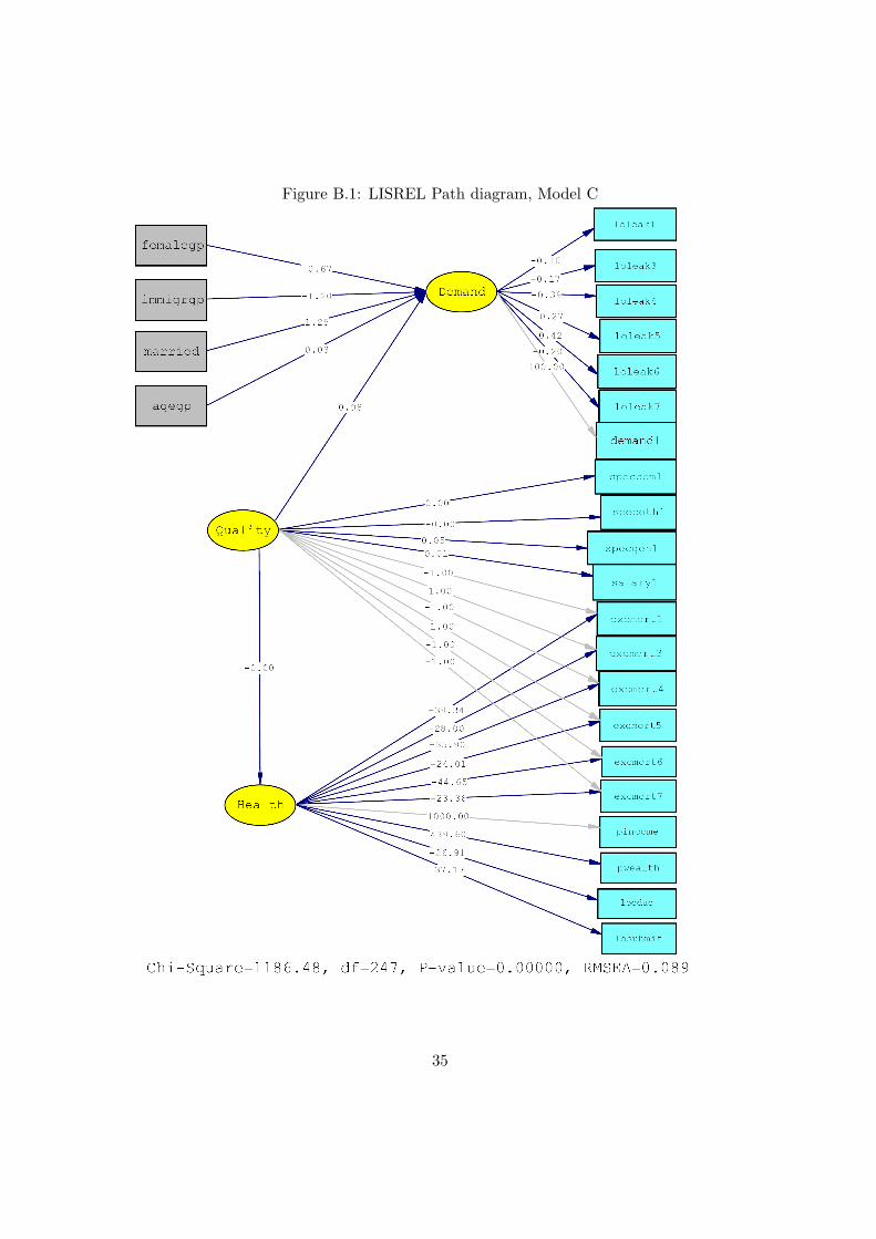
Figure B.1: LISREL Path diagram, Model C

35

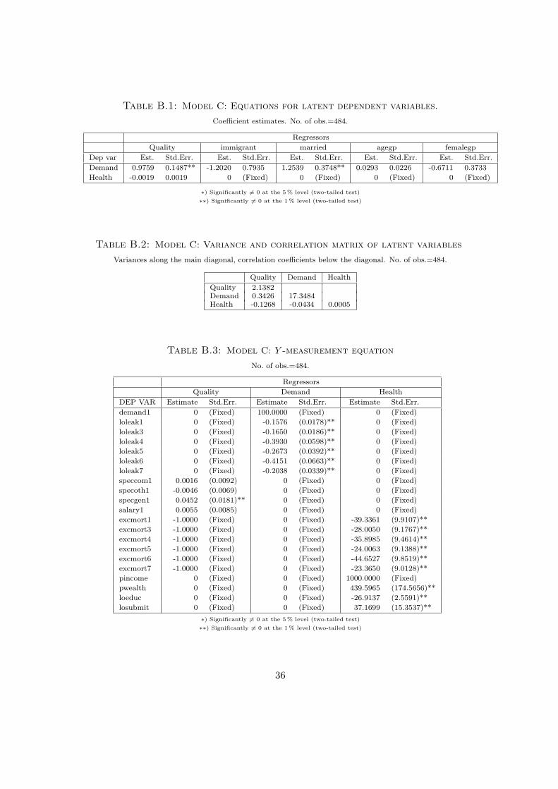
Table B.1: Model C: Equations for latent dependent variables.

Coefficient estimates. No. of obs.=484.

Regressors

Quality immigrant married agegp femalegp

Dep var Est. Std.Err. Est. Std.Err. Est. Std.Err. Est. Std.Err. Est. Std.Err.

Demand 0.9759 0.1487** -1.2020 0.7935 1.2539 0.3748** 0.0293 0.0226 -0.6711 0.3733

Health -0.0019 0.0019 0 (Fixed) 0 (Fixed) 0 (Fixed) 0 (Fixed)

∗) Significantly 6= 0 at the 5% level (two-tailed test)

∗∗) Significantly 6= 0 at the 1% level (two-tailed test)

Table B.2: Model C: Variance and correlation matrix of latent variables

Variances along the main diagonal, correlation coefficients below the diagonal. No. of obs.=484.

Quality Demand Health

Quality 2.1382Demand 0.3426 17.3484Health -0.1268 -0.0434 0.0005

Table B.3: Model C: Y -measurement equation

No. of obs.=484.

Regressors

Quality Demand Health

DEP VAR Estimate Std.Err. Estimate Std.Err. Estimate Std.Err.

demand1 0 (Fixed) 100.0000 (Fixed) 0 (Fixed)

loleak1 0 (Fixed) -0.1576 (0.0178)** 0 (Fixed)

loleak3 0 (Fixed) -0.1650 (0.0186)** 0 (Fixed)

loleak4 0 (Fixed) -0.3930 (0.0598)** 0 (Fixed)

loleak5 0 (Fixed) -0.2673 (0.0392)** 0 (Fixed)

loleak6 0 (Fixed) -0.4151 (0.0663)** 0 (Fixed)

loleak7 0 (Fixed) -0.2038 (0.0339)** 0 (Fixed)

speccom1 0.0016 (0.0092) 0 (Fixed) 0 (Fixed)

specoth1 -0.0046 (0.0069) 0 (Fixed) 0 (Fixed)

specgen1 0.0452 (0.0181)** 0 (Fixed) 0 (Fixed)

salary1 0.0055 (0.0085) 0 (Fixed) 0 (Fixed)

excmort1 -1.0000 (Fixed) 0 (Fixed) -39.3361 (9.9107)**

excmort3 -1.0000 (Fixed) 0 (Fixed) -28.0050 (9.1767)**

excmort4 -1.0000 (Fixed) 0 (Fixed) -35.8985 (9.4614)**

excmort5 -1.0000 (Fixed) 0 (Fixed) -24.0063 (9.1388)**

excmort6 -1.0000 (Fixed) 0 (Fixed) -44.6527 (9.8519)**

excmort7 -1.0000 (Fixed) 0 (Fixed) -23.3650 (9.0128)**

pincome 0 (Fixed) 0 (Fixed) 1000.0000 (Fixed)

pwealth 0 (Fixed) 0 (Fixed) 439.5965 (174.5656)**

loeduc 0 (Fixed) 0 (Fixed) -26.9137 (2.5591)**

losubmit 0 (Fixed) 0 (Fixed) 37.1699 (15.3537)**

∗) Significantly 6= 0 at the 5% level (two-tailed test)

∗∗) Significantly 6= 0 at the 1% level (two-tailed test)

36

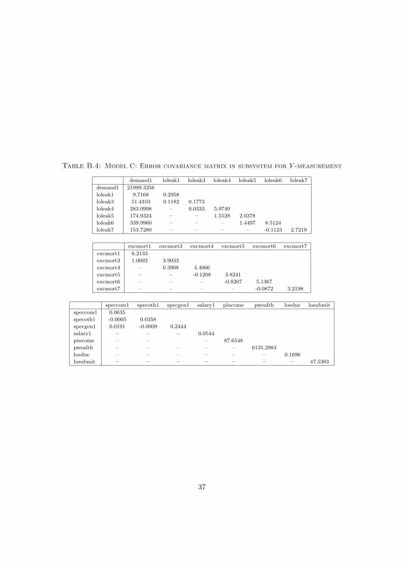
Table B.4: Model C: Error covariance matrix in subsystem for Y -measurement

demand1 loleak1 loleak3 loleak4 loleak5 loleak6 loleak7

demand1 21999.3356

loleak1 9.7168 0.2958

loleak3 51.4310 0.1182 0.1773

loleak4 283.0998 – 0.0333 5.9740

loleak5 174.9324 – – 1.5528 2.0378

loleak6 339.9960 – – – 1.4497 8.5124

loleak7 153.7280 – – – – -0.1123 2.7219

excmort1 excmort3 excmort4 excmort5 excmort6 excmort7

excmort1 6.2133

excmort3 1.0092 3.9033

excmort4 – 0.3908 4.4066

excmort5 – – -0.1208 3.8241

excmort6 – – – -0.8207 5.1367

excmort7 – – – – -0.0872 3.2198

speccom1 specoth1 specgen1 salary1 pincome pwealth loeduc losubmit

speccom1 0.0635

specoth1 -0.0005 0.0358

specgen1 0.0191 -0.0009 0.2444

salary1 – – – 0.0544

pincome – – – 87.6548

pwealth – – – – – 6131.2983

loeduc – – – – – – 0.1696

losubmit – – – – – – – 47.5383

37