1
Research MethodResearch Method
Lecture 4 (Ch5)Lecture 4 (Ch5)
OLS AsymptoticsOLS Asymptotics
©

OLS AsymptoticcOLS Asymptoticc
OLS asymptotics are the analyses of OLS properties when the sample size (n) increases to infinity. We will talk about the concept of (i) consistency and (ii) asymptotic normality.
2
ConsistencyConsistency Consistency is a similar concept as the
unbiasedness.
Unbiasedness: Given the sample size n, the expected value of the estimator is equal to the true value βj.
Consistency: The estimator approaches to the true value βj as the sample size n increases to infinity.
3
j
j
Why we need the concept Why we need the concept of consistency?of consistency?
Often, unbiasedness is difficult to achieve.
But consistency is easier to achieve under less strict conditions.
Econometrician consider that consistency is the minimum requirement for any estimators.
4
Theorem 5.1: Consistency of OLS
Under assumptions MLR.1 through MLR.4, OLS estimators is consistent for βj for j=0,1,…,k. That is:
5
j
k1,2,...,jfor )ˆlim( jjp
Proof: See front board
Consistency can be achieved under less strict assumptions, given below.
Assumptions MLR.4’
E(u)=0 and cov(xj,u)=0 for j=0,1,2,…,k
6
Asymptotic normalityAsymptotic normality In the previous handout, we assumed
that the error term is normal (MLR.6) in order to do the hypothesis testing.
But in many cases, normality assumption is not appropriate.
We want to conduct hypothesis testings while making no assumption about the distribution of the error term.
Asymptotic normality result (in the next slide) will shows that using t-test is just fine for any type of distribution.
7
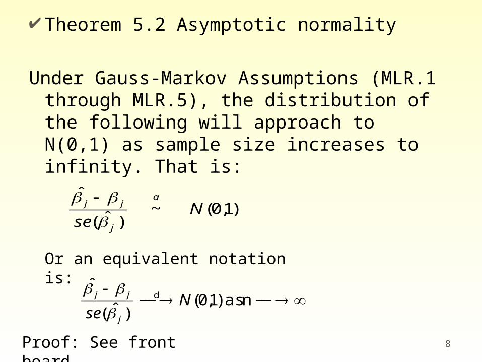
Theorem 5.2 Asymptotic normality
Under Gauss-Markov Assumptions (MLR.1 through MLR.5), the distribution of the following will approach to N(0,1) as sample size increases to infinity. That is:
8
)1,0( ~ )ˆ(
ˆN
se
a
j
jj
Or an equivalent notation is:
n as )1,0( )ˆ(
ˆd N
se j
jj
Proof: See front board
Theorem 5.2 tells us that, even if we do not know the distribution of the error term u, we can use the usual t-test in a usual way to conduct hypothesis testing.
9
Lagrange Multiplier Lagrange Multiplier Statistic (or nRStatistic (or nR22-statistic)-statistic)
Remember that F test relies on the normality assumption about u.
There is a test of the exclusion restrictions that does not need the normality assumption.
This uses LM-statistic (or often called n-R-squared statistic)
This is a test of exclusion restrictions.
10
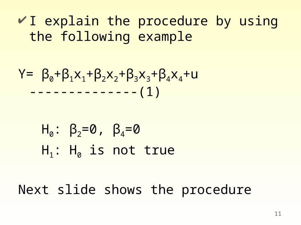
I explain the procedure by using the following example
Y= β0+β1x1+β2x2+β3x3+β4x4+u --------------(1)
H0: β2=0, β4=0
H1: H0 is not true
Next slide shows the procedure11
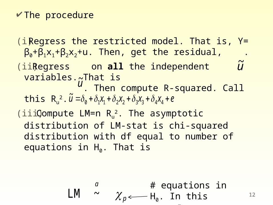
The procedure
(i)Regress the restricted model. That is, Y= β0+β1x1+β2x2+u. Then, get the residual, .
(ii)Regress on all the independent variables. That is . Then compute R-squared. Call this Ru
2.
(iii)Compute LM=n Ru2. The asymptotic
distribution of LM-stat is chi-squared distribution with df equal to number of equations in H0. That is
12
u~
exxxxu 443322110~ u~
# equations in H0. In this example q=2.p
a
~ LM
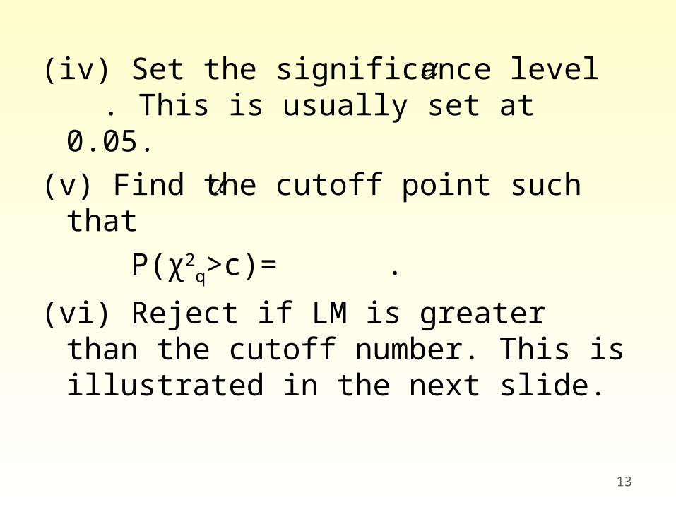
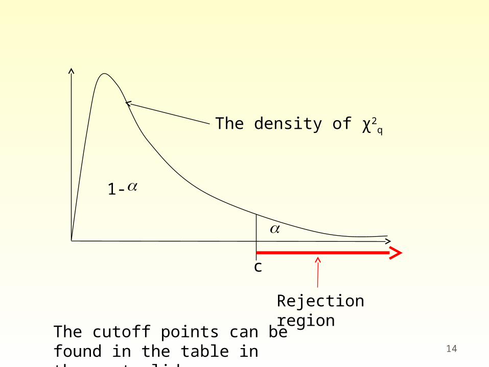
(iv) Set the significance level . This is usually set at 0.05.
(v) Find the cutoff point such that P(χ2
q>c)= .
(vi) Reject if LM is greater than the cutoff number. This is illustrated in the next slide.
13
14
c
1-
The density of χ2q
Rejection region
The cutoff points can be found in the table in the next slide.
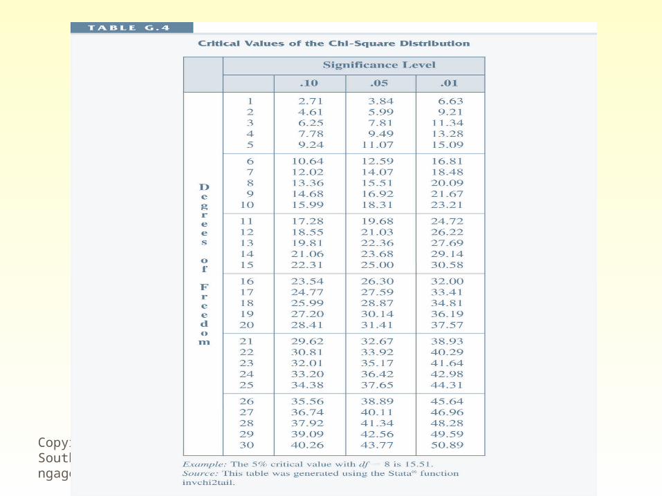
Copyright © 2009 South-Western/Cengage Learning 15
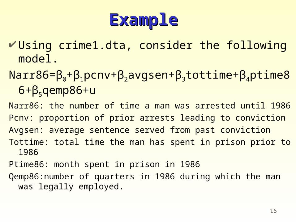
ExampleExample Using crime1.dta, consider the following
model.Narr86=β0+β1pcnv+β2avgsen+β3tottime+β4ptime86+β5q
emp86+uNarr86: the number of time a man was arrested until 1986
Pcnv: proportion of prior arrests leading to conviction
Avgsen: average sentence served from past conviction
Tottime: total time the man has spent in prison prior to 1986
Ptime86: month spent in prison in 1986
Qemp86:number of quarters in 1986 during which the man was legally employed.
16
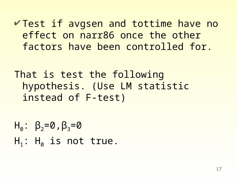
Test if avgsen and tottime have no effect on narr86 once the other factors have been controlled for.
That is test the following hypothesis. (Use LM statistic instead of F-test)
H0: β2=0,β3=0
H1: H0 is not true.
17


