1
Testing a Hypothesis about means
The contents in this chapter are from Chapter 12 to Chapter 14 of the textbook. Testing a single mean Testing two related means Testing two independent means

2
Testing a single mean
This chapter uses the gssft.sav data, which includes data for fulltime workers only.
The variables are: Hrsl: number of hours worked last week Agecat: age category Rincome: respondents income
3
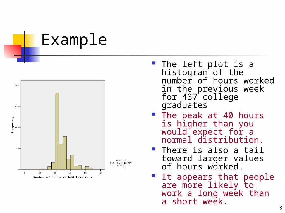
Example The left plot is a
histogram of the number of hours worked in the previous week for 437 college graduates
The peak at 40 hours is higher than you would expect for a normal distribution.
There is also a tail toward larger values of hours worked.
It appears that people are more likely to work a long week than a short week.
4
Example basic statistics
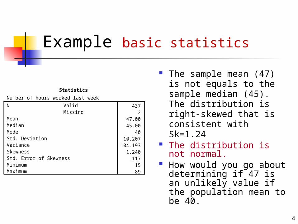
Statistics
Number of hours worked last week437
247.0045.00
4010.207
104.1931.240.117
1589
ValidMissing
N
MeanMedianModeStd. DeviationVarianceSkewnessStd. Error of SkewnessMinimumMaximum
The sample mean (47) is not equals to the sample median (45). The distribution is right-skewed that is consistent with Sk=1.24
The distribution is not normal.
How would you go about determining if 47 is an unlikely value if the population mean to be 40.
5
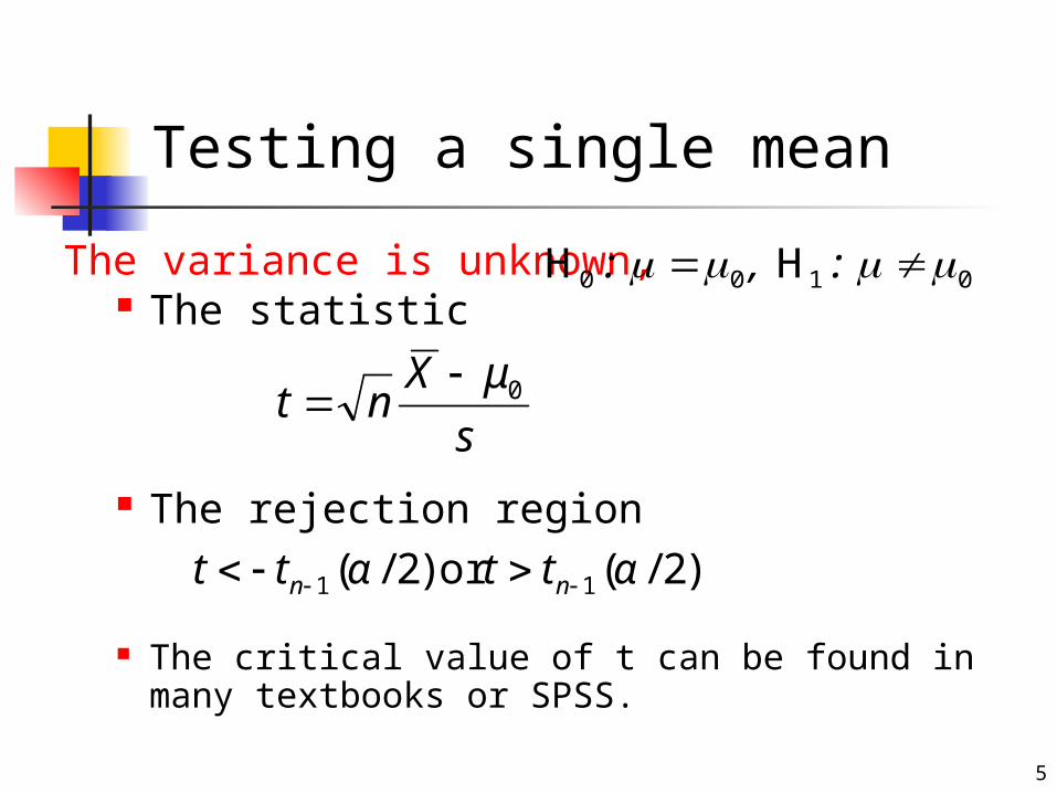
Testing a single mean
The variance is unknown, The statistic
The rejection region
The critical value of t can be found in many textbooks or SPSS.
s
μXnt 0
)2/(or )2/( 11 αttαtt nn
0100 H H :,:
6
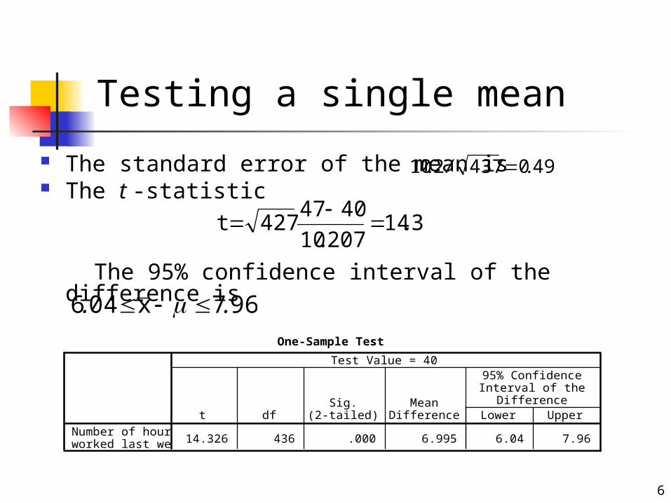
Testing a single mean
The standard error of the mean is The t -statistic
The 95% confidence interval of the difference is
490437210 ./.
One-Sample Test
14.326 436 .000 6.995 6.04 7.96Number of hoursworked last week
t dfSig.
(2-tailed)Mean
Difference Lower Upper
95% ConfidenceInterval of the
Difference
Test Value = 40
31420710
4047427t .
.
967x046 ..
7
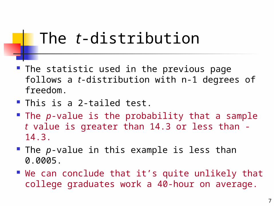
The t-distribution
The statistic used in the previous page follows a t-distribution with n-1 degrees of freedom.
This is a 2-tailed test. The p-value is the probability that a sample t value
is greater than 14.3 or less than -14.3. The p-value in this example is less than 0.0005. We can conclude that it’s quite unlikely that
college graduates work a 40-hour on average.
8
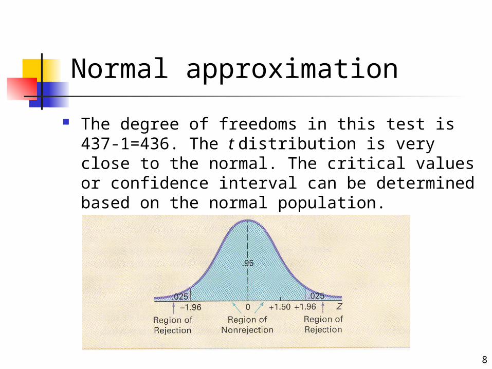
Normal approximation
The degree of freedoms in this test is 437-1=436. The t distribution is very close to the normal. The critical values or confidence interval can be determined based on the normal population.
99
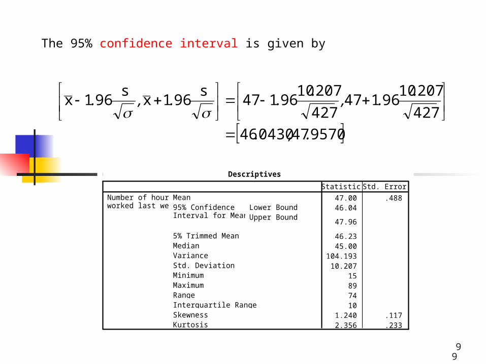
The 95% confidence interval is given by
957047043046
427
2071096147
427
2071096147
s961x
s961x
.,.
..,
...,.
Descriptives
47.00 .48846.04
47.96
46.2345.00
104.19310.207
15897410
1.240 .1172.356 .233
MeanLower BoundUpper Bound
95% ConfidenceInterval for Mean
5% Trimmed MeanMedianVarianceStd. DeviationMinimumMaximumRangeInterquartile RangeSkewnessKurtosis
Number of hoursworked last week
Statistic Std. Error
10
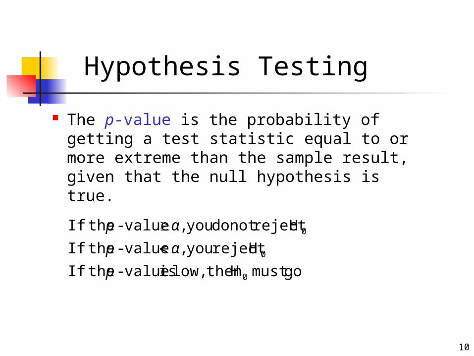
Hypothesis Testing
The p-value is the probability of getting a test statistic equal to or more extreme than the sample result, given that the null hypothesis is true.
gomust H then low, is value- theIf
Hreject you , value- theIf
Hreject not doyou , value- theIf
0
0
0
p
αp
αp
11
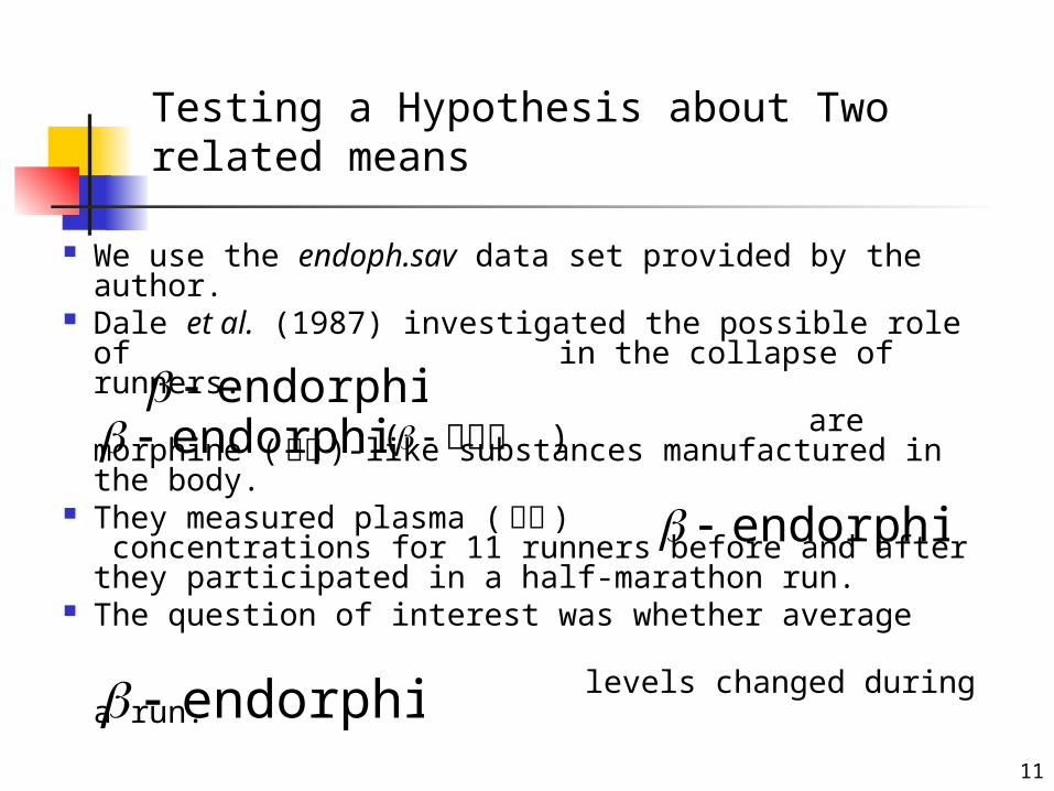
Testing a Hypothesis about Two related means
We use the endoph.sav data set provided by the author.
Dale et al. (1987) investigated the possible role of in the collapse of runners.
are morphine ( 吗啡 )-like substances manufactured in the body.
They measured plasma ( 血浆 ) concentrations for 11 runners before and after they participated in a half-marathon run.
The question of interest was whether average
levels changed during a run.endorphins
endorphins
endorphinsendorphins
)( 内啡肽
12
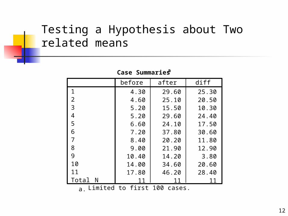
Testing a Hypothesis about Two related means
Case Summariesa
4.30 29.60 25.304.60 25.10 20.505.20 15.50 10.305.20 29.60 24.406.60 24.10 17.507.20 37.80 30.608.40 20.20 11.809.00 21.90 12.90
10.40 14.20 3.8014.00 34.60 20.6017.80 46.20 28.40
11 11 11
1234567891011
NTotal
before after diff
Limited to first 100 cases.a.

13
Testing a Hypothesis about Two related means
This problem is recommended to use the paired-samples t test.
One-Sample Statistics
11 18.7364 8.32974 2.51151diffN Mean
Std.Deviation
Std. ErrorMean
One-Sample Test
7.460 10 .000 18.73636 13.1404 24.3324difft df
Sig.(2-tailed)
MeanDifference Lower Upper
95% ConfidenceInterval of the
Difference
Test Value = 0

14
Testing a Hypothesis about Two related means
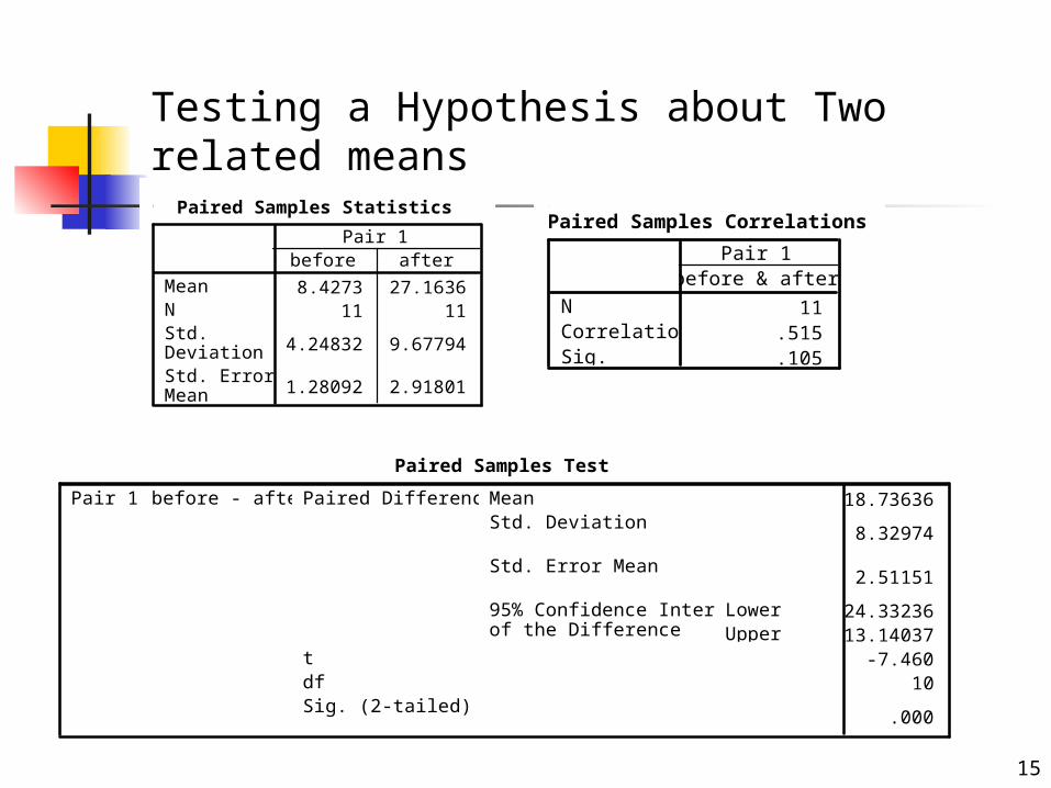
The average difference is 18.74 that is large comparing with S.D.=8.3.
The 95% confidence interval for the average difference is (13.14, 24.33) that does not includes the value of o, you can reject the hypothesis.
An equivalent way or testing the hypothesis is the t test. The p-value is less than 0.0005, we should reject the hypothesis.
15
Testing a Hypothesis about Two related means
Paired Samples Statistics
8.4273 27.163611 11
4.24832 9.67794
1.28092 2.91801
MeanNStd.DeviationStd. ErrorMean
before afterPair 1
Paired Samples Correlations
11.515.105
NCorrelationSig.
before & afterPair 1
Paired Samples Test
-18.73636
8.32974
2.51151
-24.33236-13.14037
-7.46010
.000
MeanStd. Deviation
Std. Error Mean
LowerUpper
95% Confidence Intervalof the Difference
Paired Differences
tdfSig. (2-tailed)
before - afterPair 1

16
diff Stem-and-Leaf Plot Frequency Stem & Leaf 1.00 0 . 3 4.00 1 . 0127 5.00 2 . 00458 1.00 3 . 0 Stem width: 10.00 Each leaf: 1 case (s)Each difference uses only the first two digits with
rounding.
Testing a Hypothesis about Two related means

17
All the differences are positive. That is, the after values are always greater than the before values.
The stem-and-leaf plot doesn’t suggest any obvious departures from normality.
A normal probability plot, or Q-Q plot, can helps us to test the normality of the data.
Testing a Hypothesis about Two related means
18
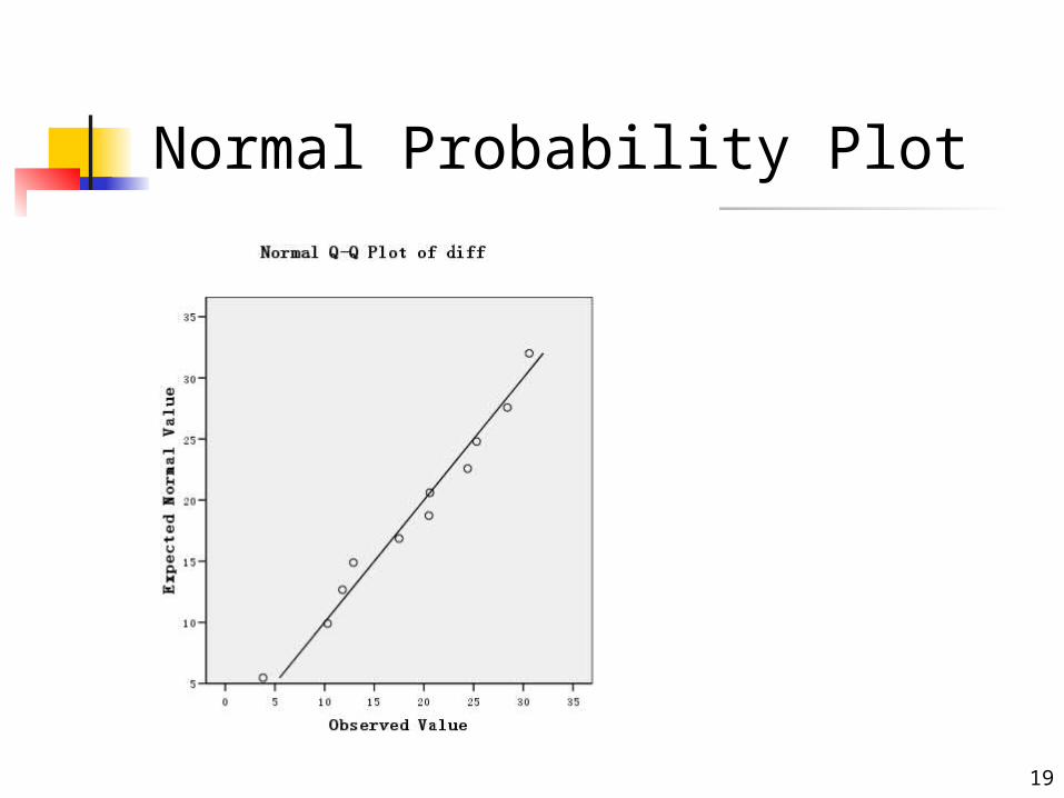
Normal Probability Plot
For each data point, the Q-Q plot shows the observed value and the value that is expected if the data are a sample from a normal distribution.
The points should cluster around a straight line if the data are from a normal distribution.
The normal Q-Q plot of the difference variable is nor or less linear, so the assumption of normality appears to be reasonable.
19
Normal Probability Plot

20
Testing Two Independent Means
This section uses the gss.sav data set.
Consider the number of hours of television viewing per day reported by internet users and non-users.
It is clear that both are not from a normal distribution.

21
Testing Two Independent Means
We find that there are some problems in the data. There are people who report watching television
for 24 hours a day!! It is impossible. Watch TV is not a very well-defined term. If you
have the TV on while you are doing homework, are you studying or watching TV?
The observations in these two groups are independent. This fact implies “two independent means”.

22
Testing Two Independent Means
Descriptives
3.52 2.423.26 2.22
3.77 2.63
3.22 2.183.00 2.00
7.801 4.6042.793 2.146
0 024 2024 202 2
2.164 3.0667.946 16.086.128 .106.112 .120.224 .240
MeanLower BoundUpper Bound
95% ConfidenceInterval for Mean
5% Trimmed MeanMedianVarianceStd. DeviationMinimumMaximumRangeInterquartile RangeSkewnessKurtosisMeanSkewnessKurtosis
Statistic
Std. Error
Hours per daywatching TV
No YesUse Internet?

23
Testing Two Independent Means
Two sample means, 2.42 hours of TV viewing and 3.52 hours for those who don’t use the internet. A difference is about 1.1 hours.
The 5% trimmed means, which are calculated by removing the top and bottom 5% of the values, are 0.3 hours less for both groups than the arithmetic means. The trimmed means are more meaningful in this case study.

24
Testing Two Independent Means
For testing the hypothesis
There are several cases:
unknown are ,
unknown are
but known, are and
known are
21
21
2121
21
211210 , μ: μHμ: μH

25
Testing Two Independent Means
)1,0(~)()(
2
22
1
21
2121 N
n
σ
n
σ
μμXXZ
2 population from taken sample theof size
2 population of variance
2 population ofmean
2 population from taken sample theofmean
1 population from taken sample theof size
1 population of variance
1 population ofmean
1 population from taken sample theofmean where
2
22
2
2
1
21
1
1
n
σ
μ
X
n
σ
μ
X

26
In most cases the variances are unknown.
Testing Two Independent Means
2
21
2
212121
~11
)()(
nn
p
t
nns
μμXXt
2 population from taken sample theof size
2 population from taken sample theof variance
2 population from taken sample theofmean
1 population from taken sample theof size
1 population from taken sample theof variance
1 population from taken sample theofmean
)1()1(
)1()1( variancepooled where
2
22
2
1
21
1
21
222
2112
n
s
X
n
s
X
nn
snsns p
27
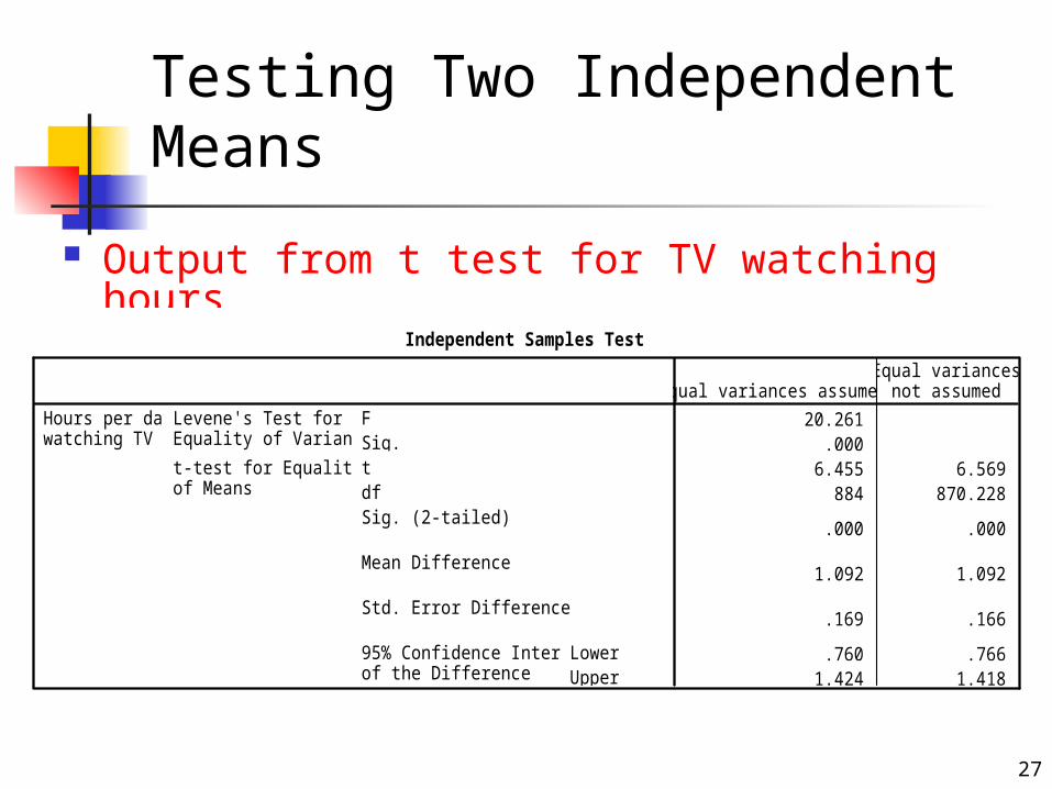
Testing Two Independent Means
Output from t test for TV watching hours
Independent Samples Test
20.261.000
6.455 6.569884 870.228
.000 .000
1.092 1.092
.169 .166
.760 .7661.424 1.418
FSig.
Levene's Test forEquality of Variances
tdfSig. (2-tailed)
Mean Difference
Std. Error Difference
LowerUpper
95% Confidence Intervalof the Difference
t-test for Equalityof Means
Hours per daywatching TV
Equal variances assumedEqual variances
not assumed

28
In the output, there are two difference versions of the t test. One makes the assumption that the variances in
the two populations are equal; the other does not.
Both tests recommend to reject the hypothesis with a significant level less than 0.0005.
The two-tailed test used in the two tests. Testing the equality of two variances will be
given next section.
Testing Two Independent Means
29
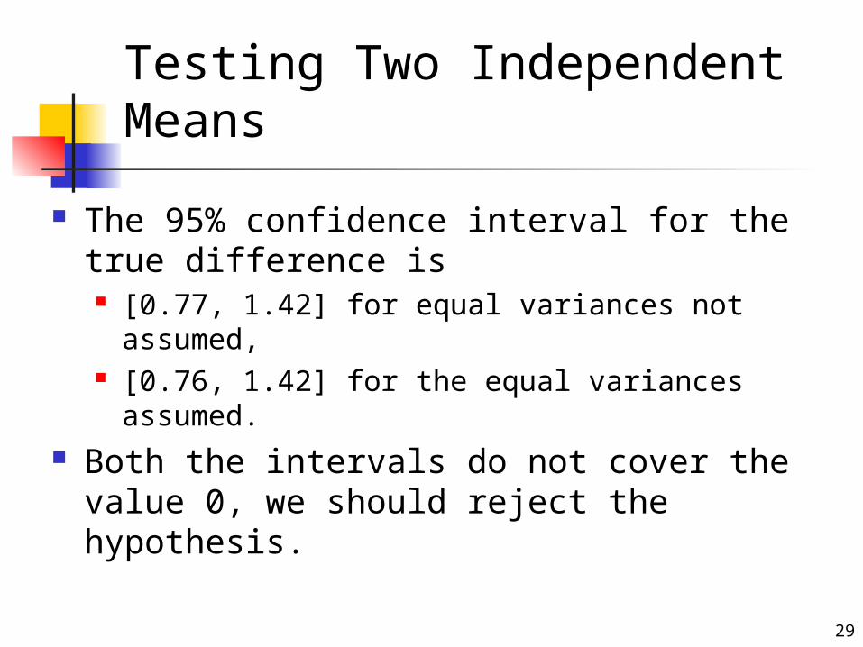
The 95% confidence interval for the true difference is [0.77, 1.42] for equal variances not assumed, [0.76, 1.42] for the equal variances assumed.
Both the intervals do not cover the value 0, we should reject the hypothesis.
Testing Two Independent Means

30
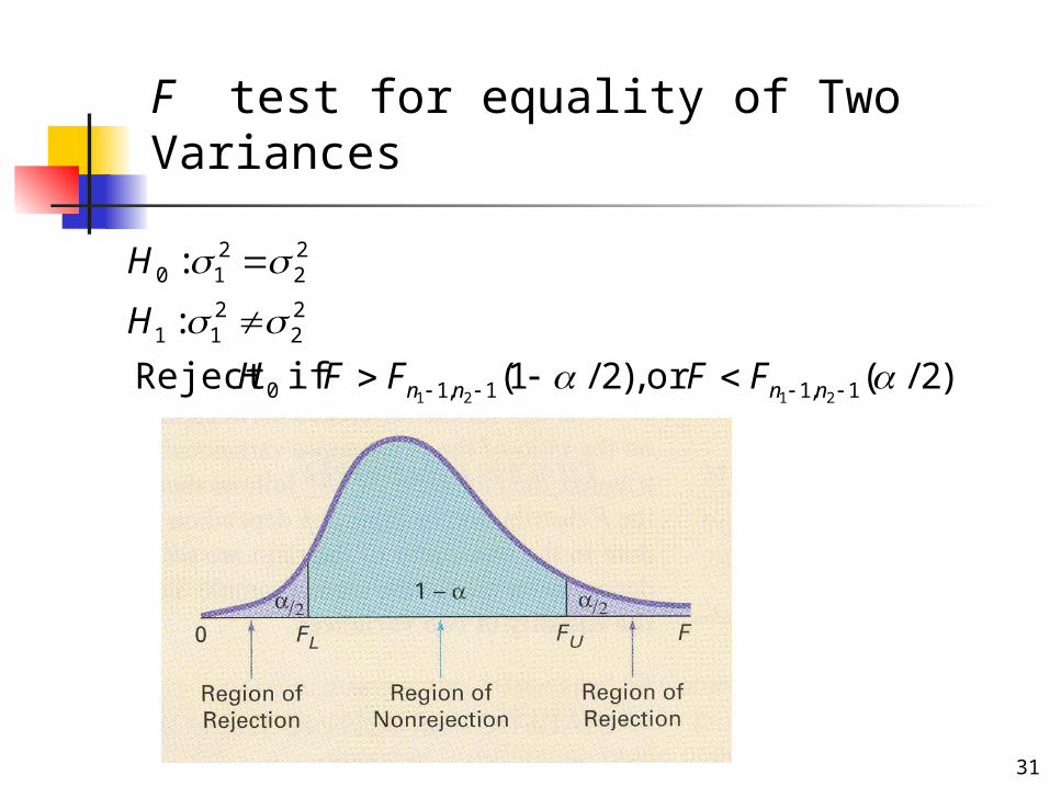
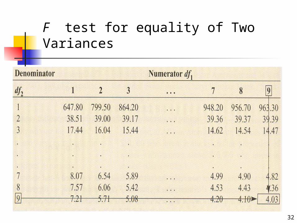
F test for equality of Two Variances
1,122
21
21~ nnF
s
sF
2 sample from freedom of degree1
1 sample from freedom of degree1
2 population from taken sample theof size
1 population from taken sample theof size
2 sample of variance
1 sample of variance where
2
1
2
1
22
21
n
n
n
n
s
s
31
F test for equality of Two Variances
)2/(or ,)2/1( if Reject
:
:
1,11,10
22
211
22
210
2121
nnnn FFFFH
H
H
32
F test for equality of Two Variances
33
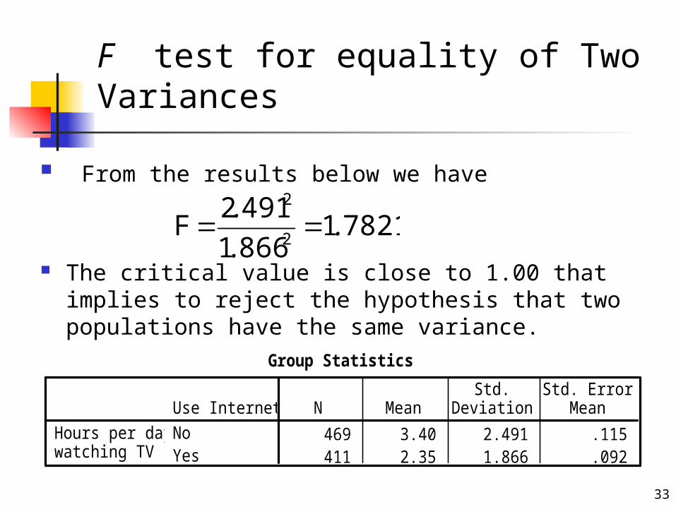
F test for equality of Two Variances
Group Statistics
469 3.40 2.491 .115411 2.35 1.866 .092
Use Internet?NoYes
Hours per daywatching TV
N MeanStd.
DeviationStd. Error
Mean
From the results below we have
The critical value is close to 1.00 that implies to reject the hypothesis that two populations have the same variance.
782118661
4912F
2
2
..
.
34
Levene’s test for equality of variances
The SPSS report used the Levene’s test (1960) that is used to test if k samples have equal variances.
Equal variances across samples is called homogeneity of variance.
The Lenene’s test is less sensitive than some other tests.
The SPSS output recommends to reject the hypothesis.

35
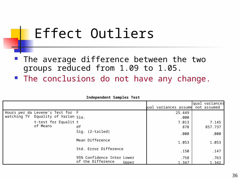
Effect Outliers
Independent Samples Test
25.449.000
7.013 7.145878 857.737
.000 .000
1.053 1.053
.150 .147
.758 .7631.347 1.342
FSig.
Levene's Test forEquality of Variances
tdfSig. (2-tailed)
Mean Difference
Std. Error Difference
LowerUpper
95% Confidence Intervalof the Difference
t-test for Equalityof Means
Hours per daywatching TV
Equal variances assumedEqual variances
not assumed
Some one reported watching TV for very long time, including 24 hours a day.
Removed observations where the person watch TV for more than 12 hours.
36
Effect Outliers
Independent Samples Test
25.449.000
7.013 7.145878 857.737
.000 .000
1.053 1.053
.150 .147
.758 .7631.347 1.342
FSig.
Levene's Test forEquality of Variances
tdfSig. (2-tailed)
Mean Difference
Std. Error Difference
LowerUpper
95% Confidence Intervalof the Difference
t-test for Equalityof Means
Hours per daywatching TV
Equal variances assumedEqual variances
not assumed
The average difference between the two groups reduced from 1.09 to 1.05.
The conclusions do not have any change.
37
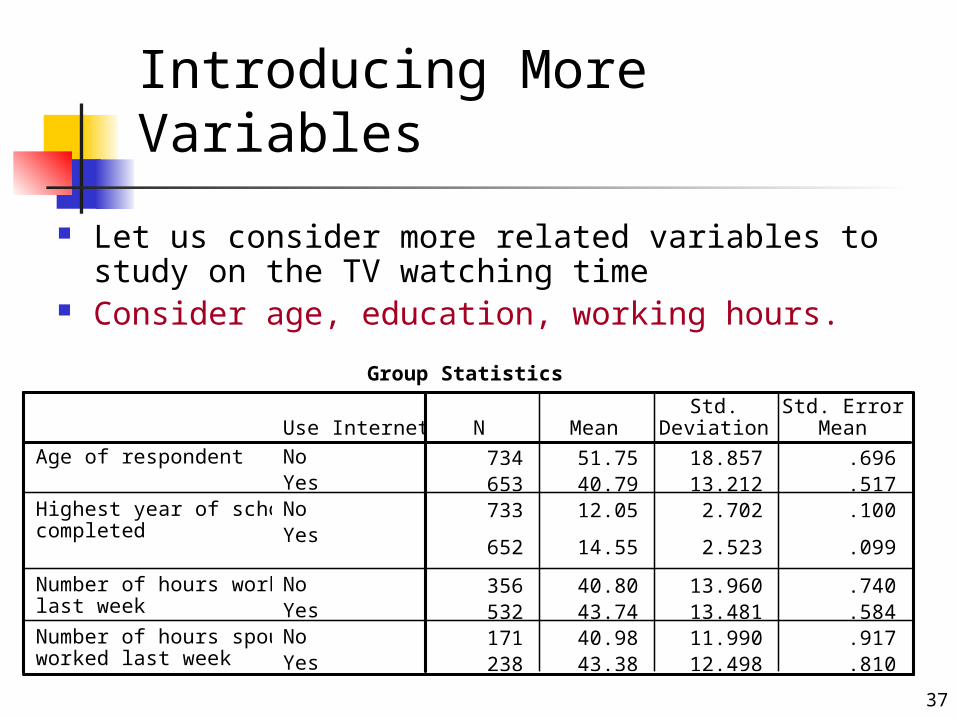
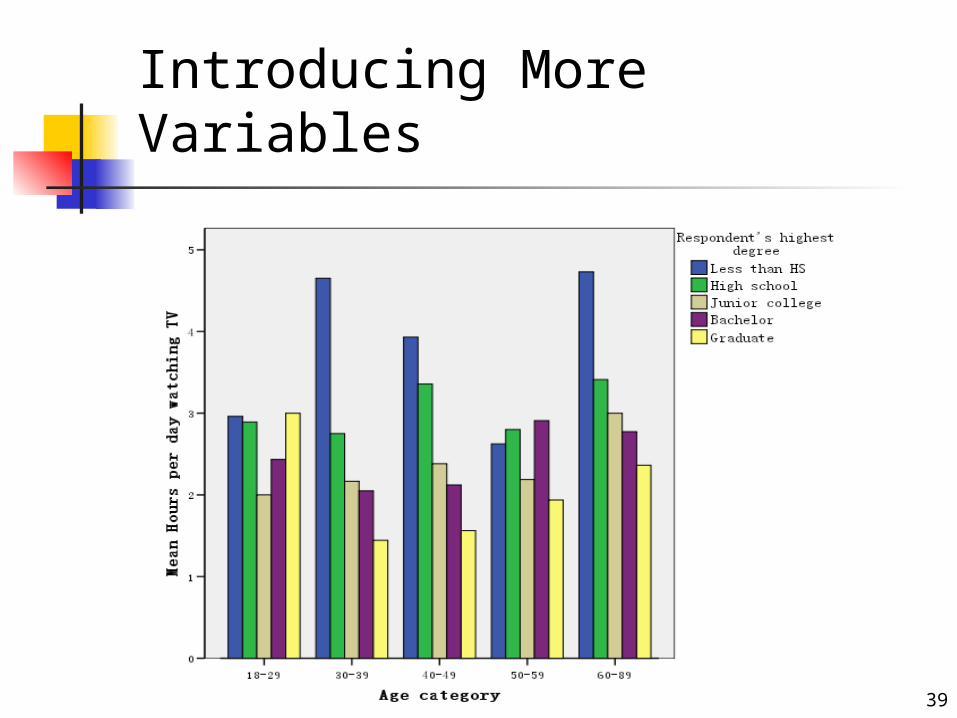
Introducing More Variables
Group Statistics
734 51.75 18.857 .696653 40.79 13.212 .517733 12.05 2.702 .100
652 14.55 2.523 .099
356 40.80 13.960 .740532 43.74 13.481 .584171 40.98 11.990 .917238 43.38 12.498 .810
Use Internet?NoYesNoYes
NoYesNoYes
Age of respondent
Highest year of schoolcompleted
Number of hours workedlast week
Number of hours spouseworked last week
N MeanStd.
DeviationStd. Error
Mean
Let us consider more related variables to study on the TV watching time
Consider age, education, working hours.
38
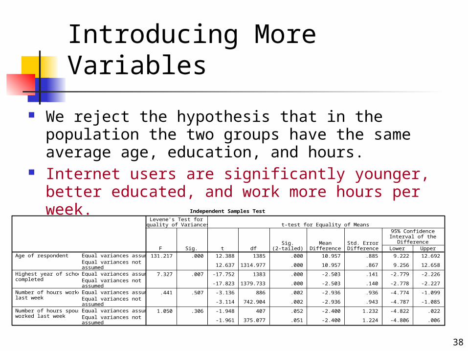
Introducing More Variables
Independent Samples Test
131.217 .000 12.388 1385 .000 10.957 .885 9.222 12.692
12.637 1314.977 .000 10.957 .867 9.256 12.658
7.327 .007 -17.752 1383 .000 -2.503 .141 -2.779 -2.226
-17.823 1379.733 .000 -2.503 .140 -2.778 -2.227
.441 .507 -3.136 886 .002 -2.936 .936 -4.774 -1.099
-3.114 742.904 .002 -2.936 .943 -4.787 -1.085
1.050 .306 -1.948 407 .052 -2.400 1.232 -4.822 .022
-1.961 375.077 .051 -2.400 1.224 -4.806 .006
Equal variances assumedEqual variances notassumedEqual variances assumedEqual variances notassumedEqual variances assumedEqual variances notassumedEqual variances assumedEqual variances notassumed
Age of respondent
Highest year of schoolcompleted
Number of hours workedlast week
Number of hours spouseworked last week
F Sig.
Levene's Test forEquality of Variances
t dfSig.
(2-tailed)Mean
DifferenceStd. ErrorDifference Lower Upper
95% ConfidenceInterval of the
Difference
t-test for Equality of Means
We reject the hypothesis that in the population the two groups have the same average age, education, and hours.
Internet users are significantly younger, better educated, and work more hours per week.
39
Introducing More Variables


