10-3 versus 10-5 polarimetry: what are the differences?
orSystematic approaches to deal with
systematic effects.
Frans SnikSterrewacht Leiden
Definitions
• Polarimetric sensitivity• Polarimetric accuracy• Polarimetric efficiency• Polarimetric precision
Polarimetric sensitivity
The noise level in Q/I, U/I, V/I above which a polarization signal can be detected.
In astronomy: signals <1% polarimetric sensitivity:
10-3 – 10-5 (or better)
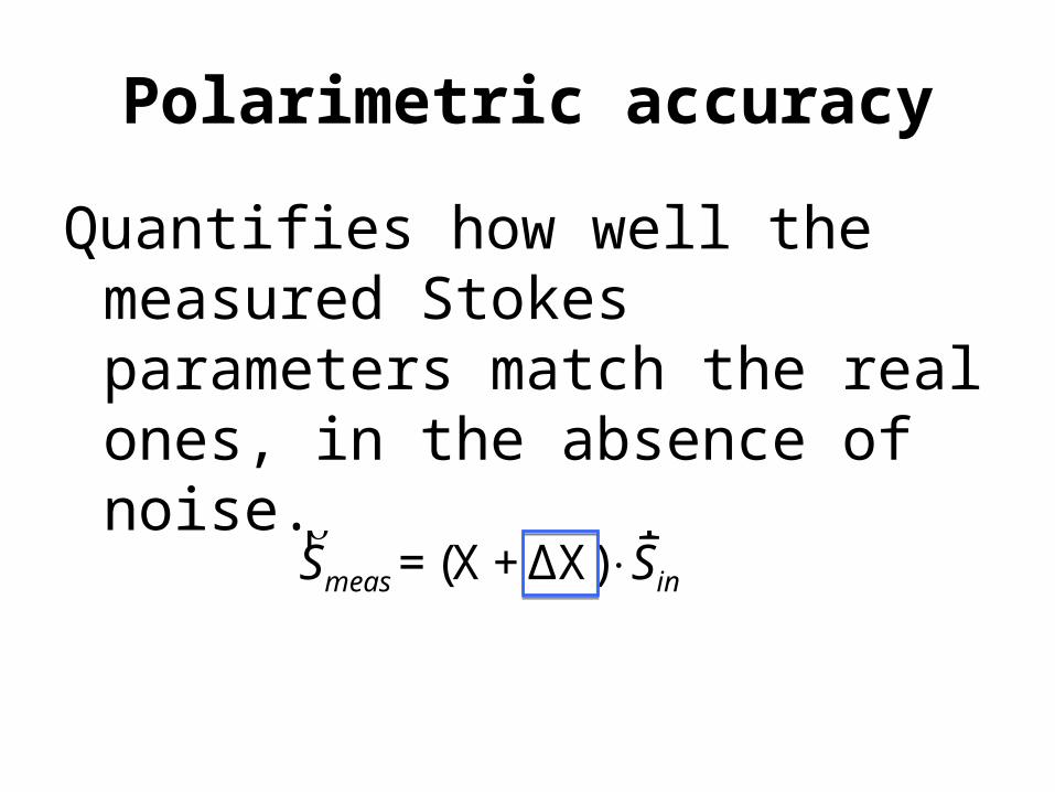
Polarimetric accuracy
Quantifies how well the measured Stokes parameters match the real ones, in the absence of noise.
€
rS meas = (X+ ΔX)⋅
r S in
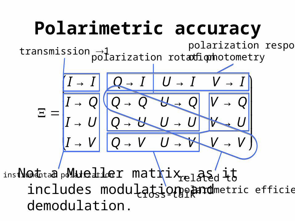
Not a Mueller matrix, as it includes modulation and demodulation.
Polarimetric accuracy
€
X =
I →I Q →I U →I V →I
I →Q Q →Q U →Q V →Q
I →U Q →U U →U V →U
I →V Q →V U →V V →V
⎛
⎝
⎜ ⎜ ⎜ ⎜
⎞
⎠
⎟ ⎟ ⎟ ⎟
transmission 1
instrumental polarization
cross-talk
polarization rotation
related topolarimetric efficiency
polarization responseof photometry
Polarimetric accuracy
€
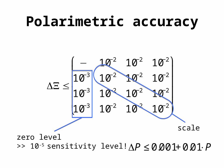
ΔX≤
− 10−2 10−2 10−2
10−3 10−2 10−2 10−2
10−3 10−2 10−2 10−2
10−3 10−2 10−2 10−2
⎛
⎝
⎜ ⎜ ⎜ ⎜
⎞
⎠
⎟ ⎟ ⎟ ⎟
zero level>> 10-5 sensitivity level!
scale
€
ΔP ≤ 0.001+ 0.01⋅ P
Polarimetric efficiency
Describes how efficiently the Stokes parameters Q, U, V are measured by employing a certain (de)modulation scheme.
1/[susceptibility to noise in demodulated Q/I, U/I, V/I]
del Toro Iniesta & Collados, Appl.Opt. 39 (2000)
Polarimetric precision
Doesn’t have any significance…
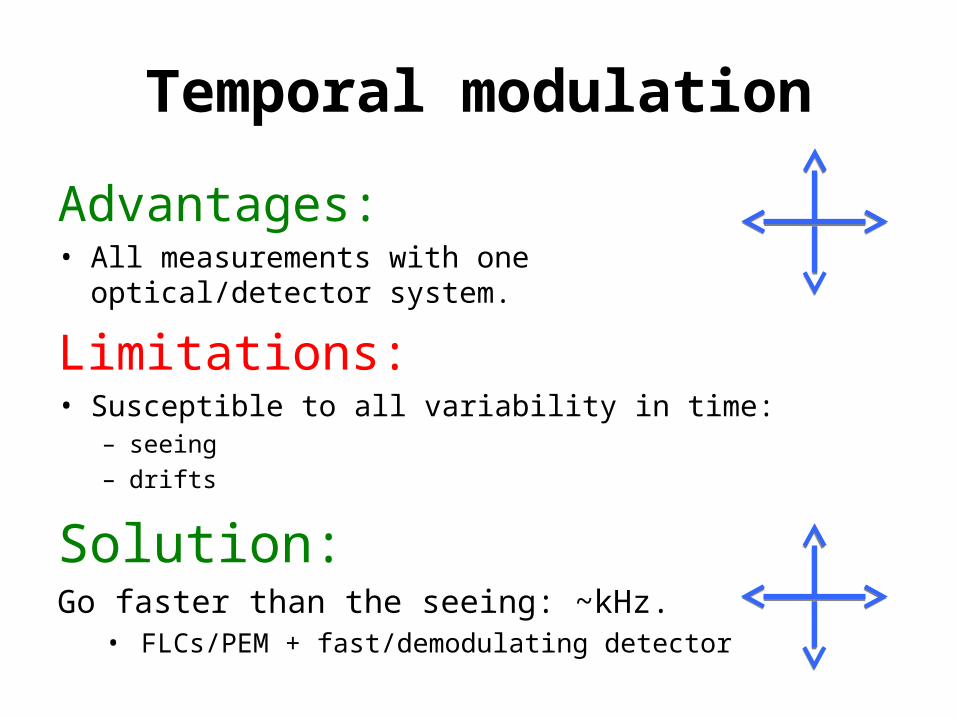
Temporal modulation
Advantages:• All measurements with one optical/detector system.
Limitations:• Susceptible to all variability in time:
– seeing– drifts
Solution:Go faster than the seeing: ~kHz.
• FLCs/PEM + fast/demodulating detector
Temporal modulation
Achievable sensitivity depends on:• Seeing (and drifts);• Modulation speed;• Spatial intensity gradients of target;• Differential aberrations/beam wobble.
Usually >>10-5
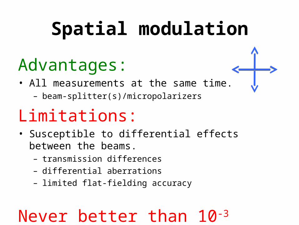
Spatial modulation
Advantages:• All measurements at the same time.
– beam-splitter(s)/micropolarizers
Limitations:• Susceptible to differential effects between the
beams.– transmission differences– differential aberrations– limited flat-fielding accuracy
Never better than 10-3
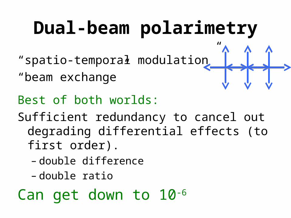
Dual-beam polarimetry
“spatio-temporal modulation”“beam exchange”
Best of both worlds:Sufficient redundancy to cancel out degrading
differential effects (to first order).– double difference– double ratio
Can get down to 10-6
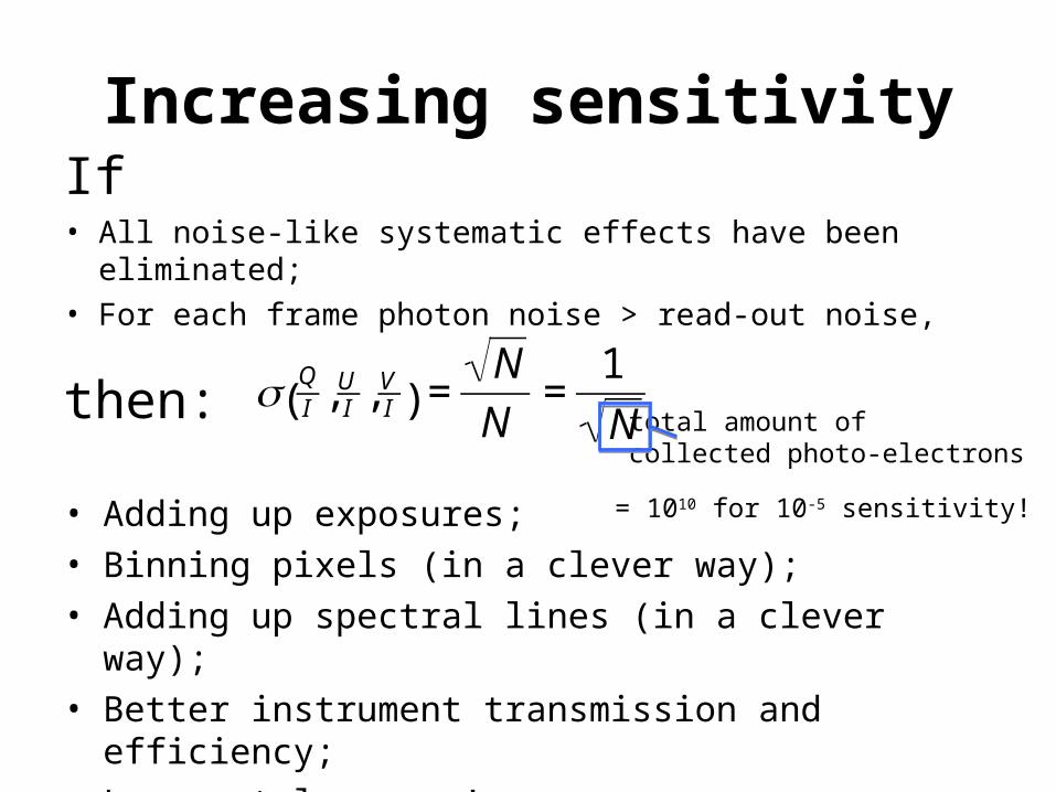
Increasing sensitivityIf• All noise-like systematic effects have been eliminated;• For each frame photon noise > read-out noise,
then:
€
σ QI ,U
I , VI( ) =
N
N=
1
N total amount of collected photo-electrons
• Adding up exposures;• Binning pixels (in a clever way);• Adding up spectral lines (in a clever way);• Better instrument transmission and efficiency;• Larger telescopes!
= 1010 for 10-5 sensitivity!
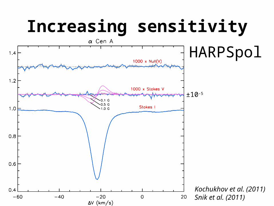
Increasing sensitivityHARPSpol
Kochukhov et al. (2011)Snik et al. (2011)
±10-5
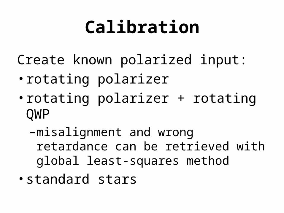
Calibration
Create known polarized input:• rotating polarizer• rotating polarizer + rotating QWP
–misalignment and wrong retardance can be retrieved with global least-squares method
• standard stars
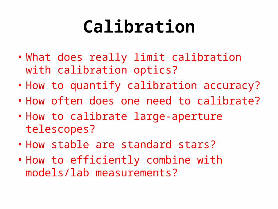
Calibration
• What does really limit calibration with calibration optics?
• How to quantify calibration accuracy?• How often does one need to calibrate?• How to calibrate large-aperture telescopes?• How stable are standard stars?• How to efficiently combine with models/lab
measurements?
Systematic effects that (still) limit polarimetric performance
• Polarized fringes• Polarized ghosts• Higher-order effects of dual-beam method• Surprising interactions
– e.g.: coupling of instrumental polarization with bias drift and detector non-linearity
• Polarized diffraction (segmented mirrors!)• System-specific effects (e.g. ZIMPOL detector) Error budgeting approach


