
1cs533d-term1-2005
NotesNotes
I am back, but still catching up Assignment 2 is due today (or next time
I’m in the dept following today) Final project proposals:
• I haven’t sorted through my email, but make sure you send me something now (even quite vague)
• Let’s make sure everyone has their project started this weekend or early next week
2cs533d-term1-2005
Multi-Dimensional Multi-Dimensional PlasticityPlasticity
Simplest model: total strain is sum of elastic and plastic parts: =e+ p
Stress only depends on elastic part(so rest state includes plastic strain):=(e)
If is too big, we yield, and transfer some of e into p so that is acceptably small

3cs533d-term1-2005
Multi-Dimensional Yield Multi-Dimensional Yield criteriacriteria
Lots of complicated stuff happens when materials yield• Metals: dislocations moving around• Polymers: molecules sliding against each other• Etc.
Difficult to characterize exactly when plasticity (yielding) starts• Work hardening etc. mean it changes all the time too
Approximations needed• Big two: Tresca and Von Mises

4cs533d-term1-2005
YieldingYielding
First note that shear stress is the important quantity• Materials (almost) never can permanently
change their volume• Plasticity should ignore volume-changing
stress So make sure that if we add kI to it
doesn’t change yield condition
5cs533d-term1-2005
Tresca yield criterionTresca yield criterion
This is the simplest description:• Change basis to diagonalize • Look at normal stresses (i.e. the eigenvalues of )
• No yield if max-min ≤ Y
Tends to be conservative (rarely predicts yielding when it shouldn’t happen)
But, not so accurate for some stress states• Doesn’t depend on middle normal stress at all
Big problem (mathematically): not smooth
6cs533d-term1-2005
Von Mises yield criterionVon Mises yield criterion
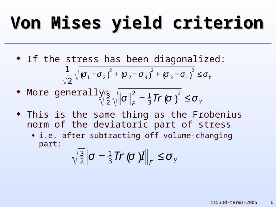
If the stress has been diagonalized:
More generally:
This is the same thing as the Frobenius norm of the deviatoric part of stress• i.e. after subtracting off volume-changing part:
€
1
2σ 1 −σ 2( )
2+ σ 2 −σ 3( )
2+ σ 3 −σ 1( )
2≤ σ Y
€
32 σ
F
2− 1
3 Tr σ( )2
≤ σ Y
€
32 σ − 1
3 Tr σ( )IF
≤ σ Y

7cs533d-term1-2005
Linear elasticity shortcutLinear elasticity shortcut
For linear (and isotropic) elasticity, apart from the volume-changing part which we cancel off, stress is just a scalar multiple of strain• (ignoring damping)
So can evaluate von Mises with elastic strain tensor too (and an appropriately scaled yield strain)

8cs533d-term1-2005
Perfect plastic flowPerfect plastic flow
Once yield condition says so, need to start changing plastic strain
The magnitude of the change of plastic strain should be such that we stay on the yield surface• I.e. maintain f()=0
(where f()≤0 is, say, the von Mises condition) The direction that plastic strain changes isn’t as
straightforward “Associative” plasticity:
€
˙ ε p = γ∂f
∂σ

9cs533d-term1-2005
AlgorithmAlgorithm
After a time step, check von Mises criterion: is ?
If so, need to update plastic strain:
• with chosen so that f(new)=0(easy for linear elasticity)
€
f (σ ) = 32 dev σ( )
F−σ Y > 0
€
pnew = ε p + γ
∂f
∂σ
= ε p + γ 32
dev(σ )
dev(σ )F
10cs533d-term1-2005
Sand (Granular Materials)Sand (Granular Materials)
Things get a little more complicated for sand, soil, powders, etc.
Yielding actually involves friction, and thus is pressure (the trace of stress) dependent
Flow rule can’t be associated See Zhu and Bridson, SIGGRAPH’05 for
quick-and-dirty hacks… :-)

11cs533d-term1-2005
Multi-Dimensional Multi-Dimensional FractureFracture
Smooth stress to avoid artifacts (average with neighbouring elements)
Look at largest eigenvalue of stress in each element
If larger than threshhold, introduce crack perpendicular to eigenvector
Big question: what to do with the mesh?• Simplest: just separate along closest mesh face• Or split elements up: O’Brien and Hodgins
SIGGRAPH’99• Or model crack path with embedded geometry:
Molino et al. SIGGRAPH’04
12cs533d-term1-2005
FluidsFluids

13cs533d-term1-2005
Fluid mechanicsFluid mechanics
We already figured out the equations of motion for continuum mechanics
Just need a constitutive model
We’ll look at the constitutive model for “Newtonian” fluids next• Remarkably good model for water, air, and many other simple
fluids• Only starts to break down in extreme situations, or more
complex fluids (e.g. viscoelastic substances)
€
ρ˙ ̇ x =∇ ⋅σ + ρg
€
= x, t,ε, ˙ ε ( )
14cs533d-term1-2005
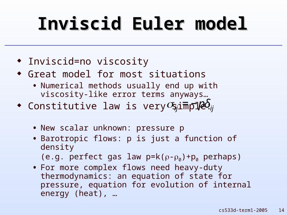
Inviscid Euler modelInviscid Euler model
Inviscid=no viscosity Great model for most situations
• Numerical methods usually end up with viscosity-like error terms anyways…
Constitutive law is very simple:
• New scalar unknown: pressure p• Barotropic flows: p is just a function of density
(e.g. perfect gas law p=k(ρ-ρ0)+p0 perhaps)
• For more complex flows need heavy-duty thermodynamics: an equation of state for pressure, equation for evolution of internal energy (heat), …
€
ij = −pδij

15cs533d-term1-2005
Lagrangian viewpointLagrangian viewpoint
We’ve been working with Lagrangian methods so far• Identify chunks of material,
track their motion in time,differentiate world-space position or velocity w.r.t. material coordinates to get forces
• In particular, use a mesh connecting particles to approximate derivatives (with FVM or FEM)
Bad idea for most fluids• [vortices, turbulence]• At least with a fixed mesh…
16cs533d-term1-2005
Eulerian viewpointEulerian viewpoint
Take a fixed grid in world space, track how velocity changes at a point
Even for the craziest of flows, our grid is always nice
(Usually) forget about object space and where a chunk of material originally came from• Irrelevant for extreme inelasticity• Just keep track of velocity, density, and whatever else
is needed
17cs533d-term1-2005
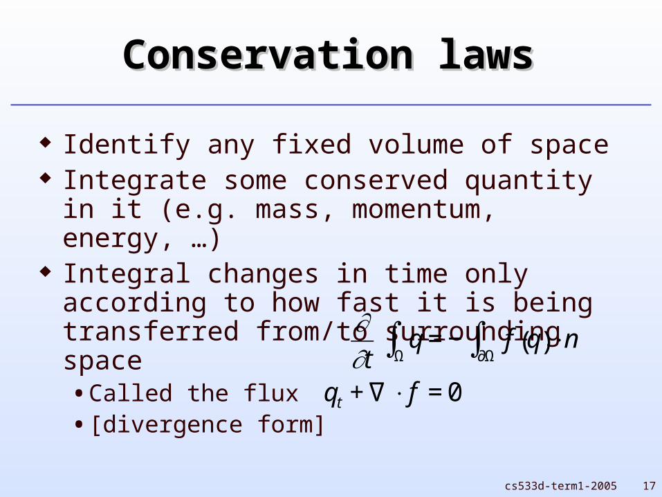
Conservation lawsConservation laws
Identify any fixed volume of space Integrate some conserved quantity in it
(e.g. mass, momentum, energy, …) Integral changes in time only according to
how fast it is being transferred from/to surrounding space• Called the flux• [divergence form]
€
∂∂t
qΩ
∫ = − f q( ) ⋅n∂Ω
∫qt +∇ ⋅ f = 0

18cs533d-term1-2005
Conservation of MassConservation of Mass
Also called the continuity equation(makes sure matter is continuous)
Let’s look at the total mass of a volume (integral of density)
Mass can only be transferred by moving it: flux must be ρu
€
∂∂t
ρΩ
∫ = − ρu ⋅n∂Ω
∫ρ t +∇ ⋅ ρu( ) = 0
19cs533d-term1-2005
Material derivativeMaterial derivative
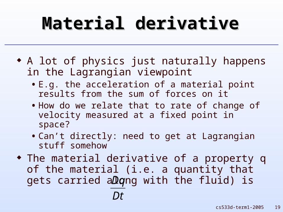
A lot of physics just naturally happens in the Lagrangian viewpoint• E.g. the acceleration of a material point results from
the sum of forces on it• How do we relate that to rate of change of velocity
measured at a fixed point in space?• Can’t directly: need to get at Lagrangian stuff
somehow The material derivative of a property q of the
material (i.e. a quantity that gets carried along with the fluid) is
€
Dq
Dt

20cs533d-term1-2005
Finding the material Finding the material derivativederivative
Using object-space coordinates p and map x=X(p) to world-space, then material derivative is just
Notation: u is velocity (in fluids, usually use u but occasionally v or V, and components of the velocity vector are sometimes u,v,w)
€
D
Dtq(t, x) =
d
dtq t, X(t, p)( )
=∂q
∂t+∇q ⋅
∂x
∂t= qt + u ⋅∇q
21cs533d-term1-2005
Compressible FlowCompressible Flow
In general, density changes as fluid compresses or expands
When is this important?• Sound waves (and/or high speed flow where motion is getting
close to speed of sound - Mach numbers above 0.3?)• Shock waves
Often not important scientifically, almost never visually significant• Though the effect of e.g. a blast wave is visible! But the shock
dynamics usually can be hugely simplified for graphics

22cs533d-term1-2005
Incompressible flowIncompressible flow
So we’ll just look at incompressible flow, where density of a chunk of fluid never changes• Note: fluid density may not be constant
throughout space - different fluids mixed together…
That is, Dρ/Dt=0
23cs533d-term1-2005
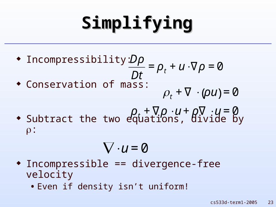
SimplifyingSimplifying
Incompressibility:
Conservation of mass:
Subtract the two equations, divide by ρ:
Incompressible == divergence-free velocity• Even if density isn’t uniform!
€
Dρ
Dt= ρ t + u ⋅∇ρ = 0
€
ρt +∇ ⋅ ρu( ) = 0
ρ t +∇ρ ⋅u + ρ∇ ⋅u = 0
€
∇⋅u = 0

24cs533d-term1-2005
Conservation of Conservation of momentummomentum
Short cut: in
use material derivative:
Or go by conservation law, with the flux due to transport of momentum and due to stress: • Equivalent, using conservation of mass
€
ρ˙ ̇ x =∇ ⋅σ + ρg
€
ρ Du
Dt=∇ ⋅σ + ρg
ρ ut + u ⋅∇u( ) =∇ ⋅σ + ρg
€
ρu( )t+∇ ⋅ uρu −σ( ) = ρg
25cs533d-term1-2005
Inviscid momentum Inviscid momentum equationequation
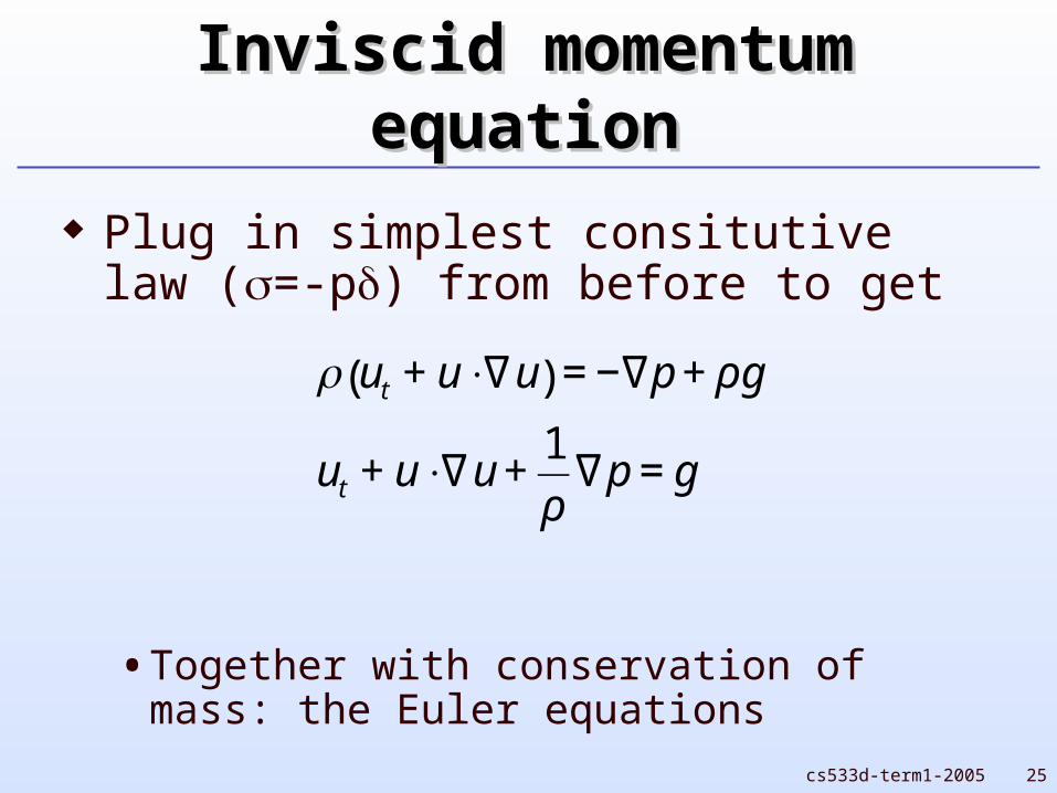
Plug in simplest consitutive law (=-p) from before to get
• Together with conservation of mass: the Euler equations€
ρ ut + u ⋅∇u( ) = −∇p + ρg
ut + u ⋅∇u +1
ρ∇p = g

26cs533d-term1-2005
Incompressible inviscid Incompressible inviscid flowflow
So the equations are:
4 equations, 4 unknowns (u, p) Pressure p is just whatever it takes to make velocity
divergence-free• Actually a “Lagrange multiplier” for enforcing the
incompressibility constraint€
ut + u ⋅∇u + 1ρ ∇p = g
∇ ⋅u = 0

27cs533d-term1-2005
Pressure solvePressure solve
To see what pressure is, take divergence of momentum equation
For constant density, just get Laplacian (and this is Poisson’s equation)
Important numerical methods use this approach to find pressure
€
∇⋅ ut + u ⋅∇u + 1ρ ∇p − g( ) = 0
∇ ⋅ 1ρ ∇p( ) = −∇ ⋅ ut + u ⋅∇u − g( )

28cs533d-term1-2005
ProjectionProjection
Note that •ut=0 so in fact
After we add p/ρ to u•u, divergence must be zero So if we tried to solve for additional pressure, we get
zero Pressure solve is linear too Thus what we’re really doing is a projection of u•u-g
onto the subspace of divergence-free functions: ut+P(u•u-g)=0
€
∇⋅1ρ ∇p = −∇ ⋅ u ⋅∇u − g( )


