Download - 50011 - core.ac.uk
0
.
X. H. Gao and J. L. Stanford*
Department of Physics Iowa State University Ames, Iowa 50011
ABSTRACT
Low frequency oscillations with periods of approximately one to two months are found in eight years of global grids of total ozone data from the Total Ozone Mapping Spectrometer (TOMS) satellite instrument. The low frequency oscillations corroborate earlier analyses based on four years of data, on the eight-year TOMS data are presented. standing "dipole" in ozone perturbations, oscillating with 35-50 day periods over the equatorial Indian Ocean-west Pacific region. This contrasts with the eastward moving dipole reported in other data sets. The standing ozone dipole appears to be a dynamical feature associated with vertical atmospheric motions. temperature fields, large-scale standing patterns are also found in the extratropics of both hemispheres, correlated with ozone fluctuations over the equatorial west Pacific. In the Northern Hemisphere, a standing pattern is observed extending from the tropical Indian Ocean to the north Pacific, across North America, and down to the equatorial Atlantic Ocean region. This feature is most pronounced in the NH summer.
In addition, both annual and seasonal one-point correlation maps based The results clearly show a
Consistent with prior analyses based on lower stratospheric
(gAS1-CB-184759) LCU FRBCUE&C Y O E C I U A Z I G I S 189-173€5 I h ' I O l h L CZCblE CELSCBEEBIPS (loud S t a t e -
Univ, of S c i e n c e a n d lrchnclccy) 16 p CSCL O4B Unclas G3/47 01901E2
*U.S. Pulbright Scholar 1988-89, Dopartmmt of Atmorphoric, Ocoanic. and Planotary Phyricr, Univorrity of Oxford, 0x1 3PU. Unitod Kingdom; and Faculty Improvwaont Loavo, Iowa Stat. Univorrity.
1
https://ntrs.nasa.gov/search.jsp?R=19890008014 2020-03-20T03:30:14+00:00Z

1. INTRODUCTION
In recent years, considerable attention has been focused on atmospheric
ozone.
ultraviolet radiation shorter than about 290 nanometers. Secondly, this
absorption of ultraviolet radiation constitutes an important heat source in
the middle and upper atmosphere, so knowledge of the distribution of ozone
and its spatial and temporal variation is crucial for accurate modeling of the
atmosphere. Moreover, in the lower stratosphere, transport dominates the
ozone distribution; therefore ozone may be used as a quasi-conserved tracer to
provide useful information about dynamical transport in the lower
stratosphere.
In the first place, ozone protects living organisms by absorbing solar
The Total Ozone Mapping Spectrometer (TOMS) carried by the Nimbus 7
satellite measures total ozone with high spatial resolution and the
measurements have been performed since late 1978. The availability of this
relatively long time series, with near global coverage, makes the TOMS data
set suitable for the study of low frequency oscillations (periods in the range
of one to two months) and their spatial correlations. It is just these
oscillations which have recently been the focus of a considerable number of
observational and modeling investigations. (See, for example, Gao and
Stanford [1987, 1988al and the references therein.)
TOMS data have been used recently in an increasing number of
observational studies, especially those related to the depletion of ozone in
the Antarctic.
Geophysical Research Letters [1986]).
(See the special Antarctic Ozone Depletion issue of the
Tung [1986] provided a theoretical basis for suggesting that changes in
lower stratospheric temperature can lead to changes in column ozone
concentration. He also pointed out that the column density of ozone should be
2
fairly well correlated with the latitudinal as well as the longitudinal
distribution of the large-scale temperature pattern at the altitude of maximum
ozone partial pressure.
In the lower stratospheric temperature field, large-scale low frequency
oscillations with periods around 40-50 days have been observed [Gao and
S t a n f o r d , 1987, 1988al. Based on Tung's theoretical idea, low frequency
oscillations observed in the temperature field can be expected to be reflected
in total ozone measurements. A natural question then arises, viz., is there a
related low frequency oscillation in total ozone?
reported evidence for 35-50 day oscillations in TOMS data over the southeast
Pacific and southern Indian Oceans.
Sabutis e t a l . [1987]
The motivation of the present paper is to examine the characteristics of
the low frequency oscillations in the TOMS data in greater detail, using the
recalibrated TOMS data set and with time series twice the length of those used
in Sabut f s e t a l . Moreover, in the present paper we present annually averaged
and seasonal maps of spatial correlations of total ozone.
2 . DATA AND ANALYSIS
Eight years of TOMS data covering Jan. 1, 1980 through Dec. 31, 1987 are
used for this study.
deg maps constructed from area averages of high spatial resolution global
measurements.
the high latitudes of the winter hemisphere.
study to the regions equatorward of 60 degrees latitude in both hemispheres.
In these regions total ozone measurements are available year around, so that
the ozone time series data do not exhibit winter gaps.
The data were obtained in the form of daily 5 deg x 5
Due to the absence of sunlight, TOMS measurements are absent at
We have therefore restricted our
Non-overlapping, three-day means were obtained from the daily grids. The
3

three-day mean time series were then used for investigations of power spectra
at various locations and were further used for spatial correlations of the low
frequency oscillations. To simplify the computation, the total ozone n(4,X,t)
is Fourier analyzed by Fast Fourier Transformation:
(1) 407
n(+ , A 9 t) 'I zo[ Cn (4 , A ) cos unt + Sn(4 9 X>sinuntl
where w,, - 2nn/(2922 day), and 4 and X are latitude and longitude.
are Fourier coefficients of the time series.
C, and S,
Then the power spectrum Pn(4, A ) for a grid with latitude 4 and longitude
X can be obtained:
Pn(4,A> - [c:(4,A> + s:(4,A)I/mw (2)
where AF - (2922 day)-'. The calculation of correlation is also performed in the spectral domain
by using these same Fourier coefficients:
R(4,A) &[cn(r>cn(4,X) + sn(r)s,(4,X)l/[~(r)s(4,X)l ( 3 )
where 0 2 ( 4 , X ) - & c 3 4 , X ) + s:(4,A) 1 - The reference point for the correlation is denoted by (r).
are made for a band of frequencies Au.
be found in Gao and Stanford [1988b].
The correlations
Further details about the method can
3 . RESULTS
3.1 Power Spectral Densities
The power spectrum of total ozone at latitude 4 and longitude A , P n ( Q , X ) ,
is obtained from the Fourier coefficients by using formula (2).
To eliminate the effect of strong annual and semi-annual cycles, the
annual oscillation and up to its seventh harmonic were removed, and their
power replaced by the average values of their two neighboring spectral points.
4
The raw periodogram was smoothed with a 15-point running mean and the
resulting bandwidths are indicated on the figures to follow.
spectral density for total ozone in the southeast Pacific and southern Indian
Oceans are shown in Figure 1.
The power
The 35-50 day oscillations were observed at these two locations by
Sabutis et al. [1987], based on analysis of four years of TOMS data covering
1 April 1979 through 3 April 1983. Subsequent to their analysis, the TOMS
data have been carefully recalibrated [Fleig et al., 19861; furthermore, a
significantly longer data set is now available. The present investigation
utilizes this new global data set, starting with 1 January 1980 to avoid
serious data gaps prior to that date.
The power spectral density results based on eight years of TOMS data show
clear evidence for existence of the low frequency oscillation at both
locations mentioned above.
significantly longer data set, corroborate the enhanced power near 35-50 day
periods reported by Sabutis et al. [1987].
The spectra shown in Figure 1, from a
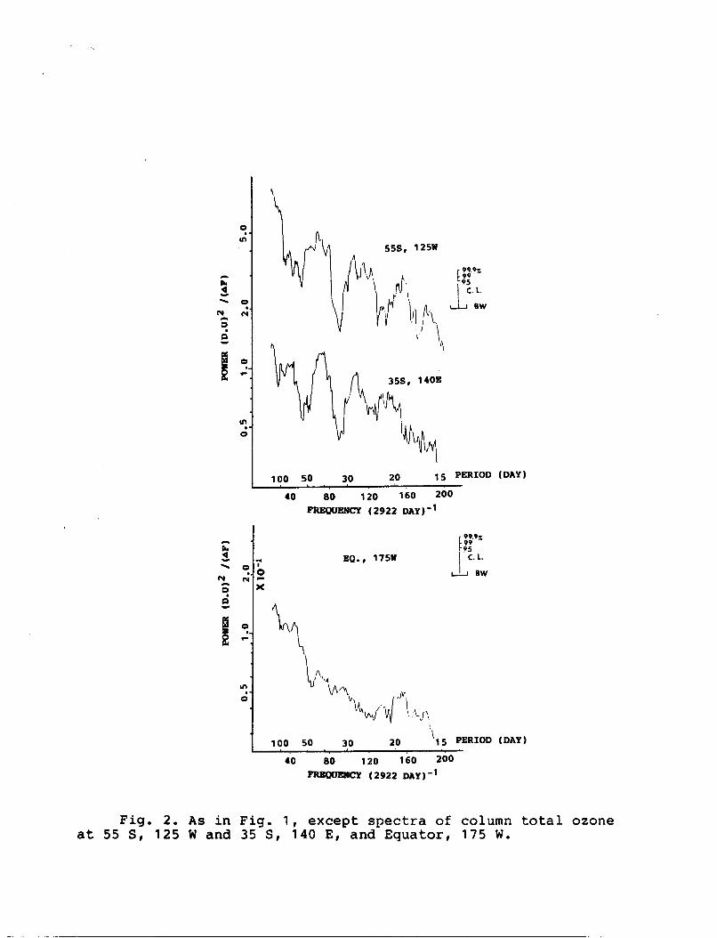
The power spectra for other regions were also investigated. In general,
the results may be summarized by saying that the spectra of total ozone over
tropical regions lack clear peaks in the low frequency range of 35 to 50 day
periods.
frequency peaks, and in many cases also show a strong peak at higher
frequency, with periods of about 22 to 28 days.
spectra are shown in Figure 2. Further study of these 22 to 28 day features is
beyond the scope of present paper.
The power spectra of middle and higher latitudes show some low
Some examples of these
3.2 Spatial Correlations
In the lower stratospheric temperature field, Cao and Stanford [1988a]
5
showed that the low frequency oscillations in extratropical regions were
statistically correlated with the oscillations in the tropics; in addition, a
possible midlatitude feedback path was observed in the correlation maps.
We have calculated similar correlation maps using eight years of TOMS
data. For comparison with the Gao and Stanford results, we have also taken
the reference point for the correlations to be located at Equator, 175 W.
in the earlier work, the zonal mean is removed. To emphasize the low frequency
features, a bell-shaped bandpass filter is used.
frequency points and has half-amplitudes at periods near 40 and 50 days.
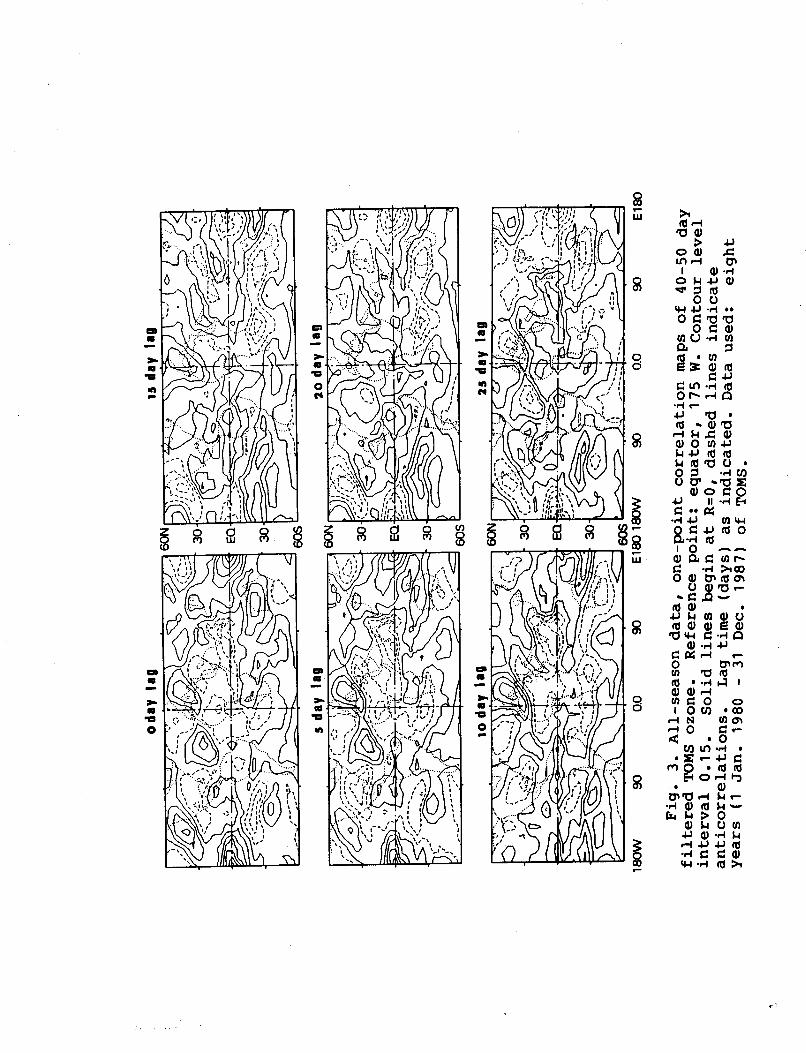
Figure 3 shows these correlation maps with various lags. Contour level
intervals of 0.15 are used in these maps.
As
The filter covers 41
The lower correlation values in Figure 3 (compared with that in
temperature field of our earlier study) is mainly due to the longer time
coverage of this data set. However, longer time series lengths increase the
temporal degrees of freedom and reduce the significance level needed for
statistical correlation.
bandpass filtered TOMS data used for the present correlation calculations is
not less than 40, and the estimated 95 percent significance level at a given
location is about 0 . 2 5 . The same methods were used here for the estimations
as those discussed in previous papers [Gao and Stanford 1988a, 1988bl.
The estimated temporal degrees of freedom for the
The previously known "dipole" structure over the equatorial Indian and
Pacific Oceans is clearly visible in Figure 3.
regions are about 90 degrees apart longitudinally, consistent with earlier
observations (for example, Lau and Chan [1985]; Weickmann et a l . [1985]; Gao
and Stanford [1988a]). However, the "dipole" structure observed here does not
show much eastward movement, in contrast with the eastward propagating dipole
feature observed in lower stratospheric temperature and out-going longwave
These two anti-correlated
6

radiation analyses.
According to Tung [1986], the basic mechanism behind the good correlation
between column ozone and lower stratospheric temperature is the vertical
motion resulting from the temperature deviations from their radiative
equilibrium value. The colder air has less radiative cooling, leading to more
net heating and results in upward motion.
motion, which is almost parallel to the gradient of ozone concentration,
creates changes in ozone mixing ratio which has its maximum located in the
stratosphere.
perhaps one should associate the standing component in the temperature
disturbance with the vertical motion and the traveling component with
longitudinal advection.
zonally symmetric ozone distribution (approximately true of the observed
tropical total ozone field, Bowman and Krueger [1985], the associated
longitudinal propagation feature does not cause a significant traveling dipole
feature in total ozone.
In the time mean, this vertical
To understand the dipole behavior observed in total ozone,
Since the longitudinal motion has no effect on a
In Figure 3, on the correlation maps with 0-, 5-, and 25-day lags, a
response pattern is observed in the Southern Hemisphere (SH) extratropical
region, consistent with the possible feedback path for low-frequency
atmospheric oscillations observed previously in lower stratosphere temperature
correlation maps [Gao and Stanford , 1988al.
In the Northern Hemisphere (NH), a relatively strong standing wave
pattern is observed, extending approximately from the tropical Indian Ocean,
to eastern China-Korea, to the North Pacific south of Alaska, over North
America, and returning to the tropical Atlantic Ocean.
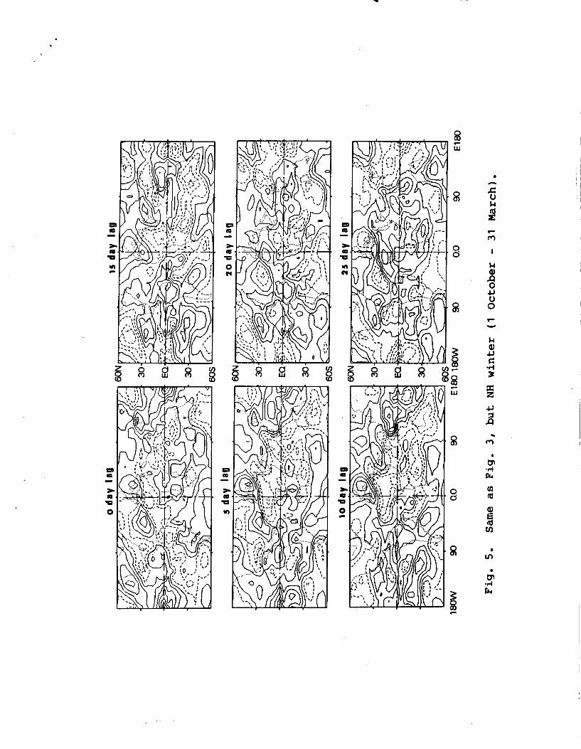
Figures 4 and 5 show the seasonal correlation maps for eight years of NH
summers (1 April - 30 September) and NH winters (1 October-30 May),
7
respectively.
in both seasons.
wave pattern is most apparent in the NH summer (Fig. 4).
may reflect different source strengths, but also seasonally varying wind
curvature effects which selectively allow or prevent propagation of the low
The tropical Indian Ocean-west Pacific dipole is clearly seen
The extratropical NH Pacific-North America-Atlantic standing
The seasonal effects
frequency signals to higher latitudes.
4. SUmARY
Low frequency oscillations with period near 35-50 days over the southeast
Pacific and southern Indian Oceans are observed in eight years of TOMS data.
The power spectral densities of total ozone over these two regions corroborate
the results reported by Sabut i s et a l . [1987] based on shorter time series.
One-point correlation maps are calculated and show a dipole feature over
the tropical Indian Ocean-west central Pacific Ocean. The dipole feature
observed in the TOMS data is located in the same region with the same period
as that observed in lower stratospheric temperature analyses. In contrast,
however, the dipole feature in the TOMS data does not show eastward
propagation and is more indicative of a standing wave phenomenon, in the
seasonal and annual means. An argument is given why ozone perturbations
should show primarily a standing dipole, whereas traveling features are found
in tropical temperature and cloud data sets.
Extratropical response patterns are visible in one-point correlation maps
and are consistent with similar features observed in lower stratospheric
temperature field analyses.
The standing component of the tropical dipole source region observed
here, in contrast with the eastward traveling dipole seen in other studies,
may offer at least a partial answer to the puzzling question of why there
exist extratropical standing waves at all, given the previously observed
eastward moving tropical source.
Acknowledgments.
Aeronautics and Space Administration under Grant NAG 5-1060 and the National
Science Foundation under Grant ATM-8722703.
Improvement Leave from Iowa State University and U. S. Fulbrfght Scholar at
the University of Oxford, United Kingdom, 1988-89.
This paper is based upon work supported by the National
The second author was on Faculty
REFERENCES
Antarctic Ozone Depletion (1986). Geophys. Res. Letts., 13, No.12, November
Supplement.
Bowman, K. P., and A. J. Krueger, A global climatology of total ozone from the
Nimbus 7 Total Ozone Mapping Spectrometer, J . Geophys. Res., 90 ,
7967-7976, 1985.
Fleig, A. J., P. K. Bhartia, C. G. Wellemeyer, and D. S. Silberstein, Seven
years of total ozone from the TOMS instrument- A report on data quality,
Geophys. Rev. Letts., 13, 1355-1358, 1986.
Gao, X. H., and J. L. Stanford, Low-frequency oscillations of the large-scale
stratospheric temperature field, J . Atmos. Scf., 44, 1991-2000, 1987.
--- , Possible feedback path for low-frequency atmospheric oscillations, J .
A t m s . Scf., 45, 1425-1432 , 1988.
--- , An efficient approach for statistical calculations with globally gridded filtered time series, J . Climate, 1 , 429-434, 1988.
Lau, K. M., and P. H. Chan, Aspects of the 40-50 day oscillation during the
northern winter as inferred from outgoing longwave radiation, Mon. Wea.
Rev., 113, 1889-1909, 1985.
Sabutis, J . L., J. L. Stanford, and K. P. Bowman, Evidence for 35-50 day low
frequency oscillations in total ozone mapping spectrometer,
Res. Lett., 9 , 945-947, 1987.
Geophys.
Tung, K. K., On the relationship between the thermal structure of the
9
stratosphere and the seasonal distribution of ozone, Geophys. Res.
Lett., 13, 1308-1311, 1986.
Weickmann, K. M., G. R. Lussky, and J. E. Kutzbach, Intraseasonal (30-60 day)
fluctuations of outgoing longwave radiation and 250 mb stream function
during northern winter, Mon. Wea. Rev . , 113, 941-961, 1985.
I C
Fig. 1. Power spectral density vs. frequency of column total ozone at 35 S,
100 W and 45 S, 20 E.
means and the resulting bandwidths (BW) are indicated. The C . L . (confidence
level) scale is based on the chi-square distribution. D.U. stands for Dobson
units and AF is defined in the text.
The spectra have been smoothed with 15-point running
Fig. 2. As in Figure 1, except spectra of column total ozone at 55 S, 125 W
and 35 S, 140 E, and Equator, 175 W.
Fig. 3. All-season data, one-point correlation maps of 40-50 day filtered
TOMS ozone. Reference point: equator, 175 W. Contour level interval 0.15.
Solid lines begin at R-0, dashed lines indicate anticorrelations.
(days) as indicated. Data used: eight years (1 Jan. 1980 - 31 Dec. 1987) of TOMS.
Lag time
Fig. 4. Same as Figure 3, but for NH summer (1 April - 30 September).
Fig. 5. Same as Figure 3, but NH winter (1 October - 31 March).
i i

10- L
40 -i
00
15 PERIOD (DAY) 0 20
99.9:: L vv
1 C . L . - 95
35s, l O O W A BW
100 50 30 20 15 PERIOD (DAY 1
F i g . 1 . Power s p e c t r a l d e n s i t y v s . frequency of column t o t a l The spec tra have been smoothed ozone a t 35 S , 100 W and 45 S , 20 E .
with 15-point running means and the r e s u l t i n g bandwidths (BW) a r e i n d i c a t e d . chi-square d i s t r i b u t i o n . i s def ined i n the t e x t .
The C.L. (conf idence l e v e l ) scale i s based on the D . U . s tands for Dobson u n i t s and AF
15 PERIOD (DAY) 100 50 30 20
40 i o 120 160 200 PREWENCY (2922 DAY)-’
I I
2 X
EQ., 175W
100 50 30 20 ‘15 PERIOD (DAY)
40 80 120 160 200 (2922 DAY1-l
Fig. 2. As in F i g . 1 , except spec tra of column t o t a l ozone a t 55 S , 1 2 5 W and 35 S , 140 E , and Equator, 175 W .

LI
k a, A 0
JJ u 0


