Download - 6 - 1 CHAPTER 6 Risk and Rates of Return Stand-alone risk Portfolio risk Risk & return: CAPM/SML

6 - 1
CHAPTER 6 Risk and Rates of Return
Stand-alone risk
Portfolio risk
Risk & return: CAPM/SML

6 - 2
What is investment risk?
Investment risk pertains to the probability of actually earning a low or negative return.
The greater the chance of low or negative returns, the riskier the investment.
6 - 3
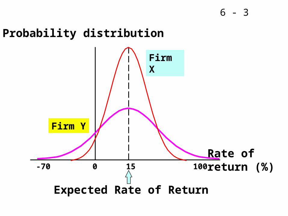
Probability distribution
Expected Rate of Return
Rate ofreturn (%)100150-70
Firm X
Firm Y
6 - 4
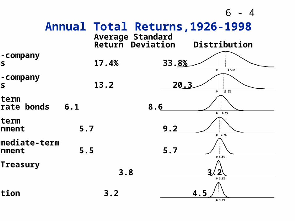
Annual Total Returns,1926-1998Average StandardReturn Deviation Distribution
Small-companystocks 17.4% 33.8%
Large-companystocks 13.2 20.3
Long-termcorporate bonds 6.1 8.6
Long-termgovernment 5.7 9.2
Intermediate-termgovernment 5.5 5.7
U.S. Treasurybills 3.8 3.2
Inflation 3.2 4.5
0 17.4%
0 13.2%
0 6.1%
0 5.7%
0 5.5%
0 3.8%
0 3.2%
6 - 5
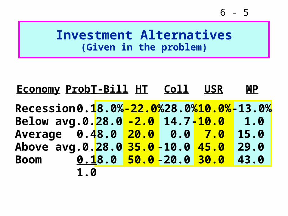
Investment Alternatives(Given in the problem)
Economy Prob. T-Bill HT Coll USR MP
Recession 0.1 8.0% -22.0% 28.0% 10.0% -13.0%Below avg. 0.2 8.0 -2.0 14.7 -10.0 1.0Average 0.4 8.0 20.0 0.0 7.0 15.0Above avg. 0.2 8.0 35.0 -10.0 45.0 29.0Boom 0.1 8.0 50.0 -20.0 30.0 43.0
1.0
6 - 6
Why is the T-bill return independent of the economy?
Will return the promised 8% regardless of the economy.

6 - 7
Do T-bills promise a completelyrisk-free return?
No, T-bills are still exposed to the risk of inflation.
However, not much unexpected inflation is likely to occur over a relatively short period.

6 - 8
Do the returns of HT and Coll. move with or counter to the economy?
HT: Moves with the economy, and has a positive correlation. This is typical.
Coll: Is countercyclical of the economy, and has a negative correlation. This is unusual.
6 - 9
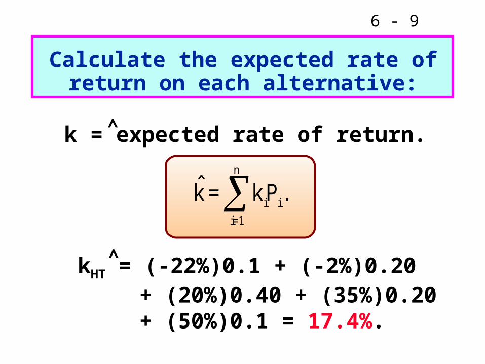
Calculate the expected rate of return on each alternative:
.Pk = k̂n
1=i
iik = expected rate of return.
kHT = (-22%)0.1 + (-2%)0.20 + (20%)0.40 + (35%)0.20 + (50%)0.1 = 17.4%.
^
^

6 - 10
k
HT 17.4%
Market 15.0
USR 13.8
T-bill 8.0
Coll. 1.7
HT appears to be the best, but is it really?
^

6 - 11
What’s the standard deviationof returns for each alternative?
= Standard deviation.
= =
=
Variance 2
.P)k̂k(n
1ii
2i

6 - 12
T-bills = 0.0%.HT = 20.0%.
Coll = 13.4%.USR = 18.8%. M = 15.3%.
1/2
T-bills =
.P)k̂k(n
1ii
2
i
(8.0 – 8.0)20.1 + (8.0 – 8.0)20.2
+ (8.0 – 8.0)20.4 + (8.0 – 8.0)20.2
+ (8.0 – 8.0)20.1

6 - 13
Prob.
Rate of Return (%)
T-bill
USR
HT
0 8 13.8 17.4

6 - 14
Standard deviation (i) measures total, or stand-alone, risk.
The larger the i , the lower the probability that actual returns will be close to the expected return.

6 - 15
Expected Returns vs. Risk
SecurityExpected
return Risk,
HT 17.4% 20.0%Market 15.0 15.3USR 13.8* 18.8*T-bills 8.0 0.0Coll. 1.7* 13.4*
*Seems misplaced.
6 - 16
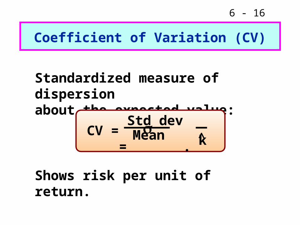
Coefficient of Variation (CV)
Standardized measure of dispersionabout the expected value:
Shows risk per unit of return.
CV = = . Std dev
k̂Mean
6 - 17
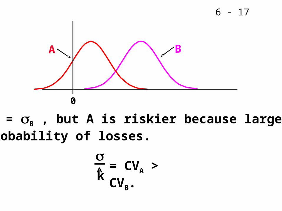
0
A B
A = B , but A is riskier because largerprobability of losses.
= CVA > CVB.k̂

6 - 18
Portfolio Risk and Return
Assume a two-stock portfolio with $50,000 in HT and $50,000 in Collections.
Calculate kp and p.^
6 - 19
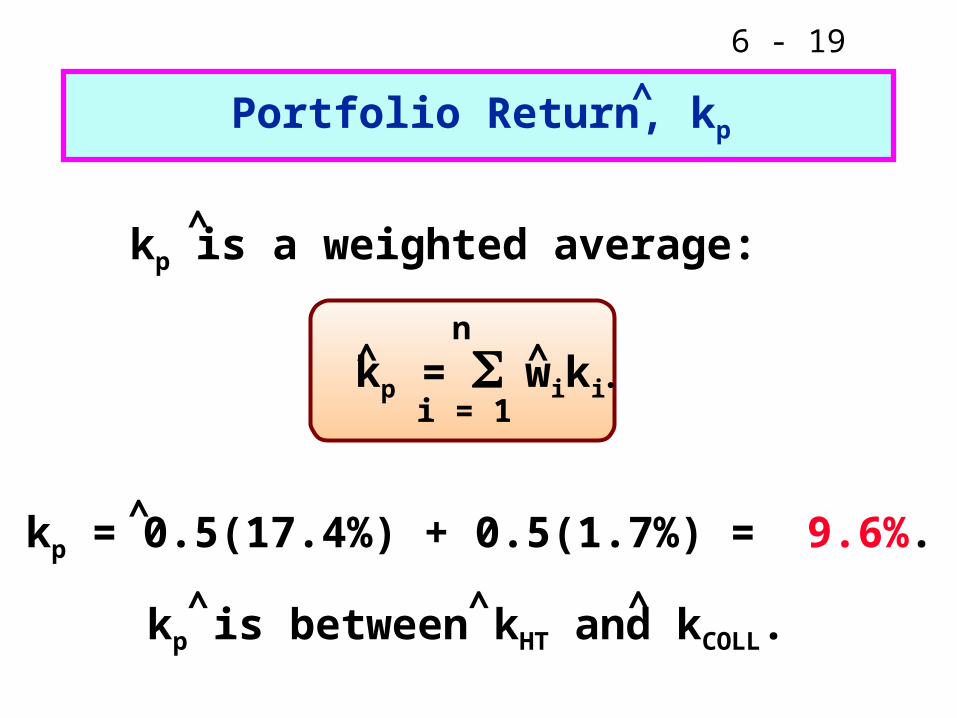
Portfolio Return, kp
kp is a weighted average:
kp = 0.5(17.4%) + 0.5(1.7%) = 9.6%.
kp is between kHT and kCOLL.
^
^
^
^
^ ^
^ ^
kp = wikin
i = 1
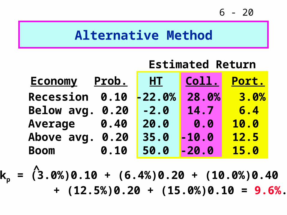
6 - 20
Alternative Method
kp = (3.0%)0.10 + (6.4%)0.20 + (10.0%)0.40 + (12.5%)0.20 + (15.0%)0.10 = 9.6%.
^
Estimated Return
Economy Prob. HT Coll. Port.
Recession 0.10 -22.0% 28.0% 3.0%Below avg. 0.20 -2.0 14.7 6.4Average 0.40 20.0 0.0 10.0Above avg. 0.20 35.0 -10.0 12.5Boom 0.10 50.0 -20.0 15.0
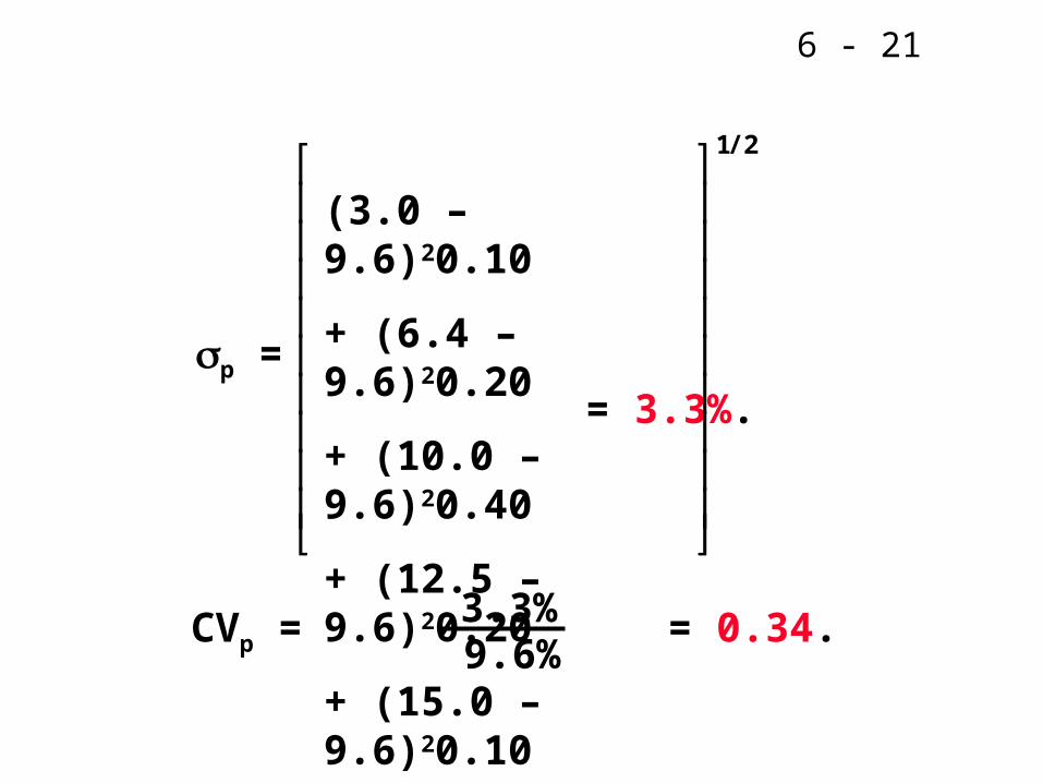
6 - 21
CVp = = 0.34. 3.3% 9.6%
p = = 3.3%.
1 2/
(3.0 – 9.6)20.10
+ (6.4 – 9.6)20.20
+ (10.0 – 9.6)20.40
+ (12.5 – 9.6)20.20
+ (15.0 – 9.6)20.10

6 - 22
p = 3.3% is much lower than that of
either stock (20% and 13.4%).
p = 3.3% is lower than average of HT
and Coll = 16.7%.
Portfolio provides average k but lower risk.
Reason: negative correlation.
^
6 - 23
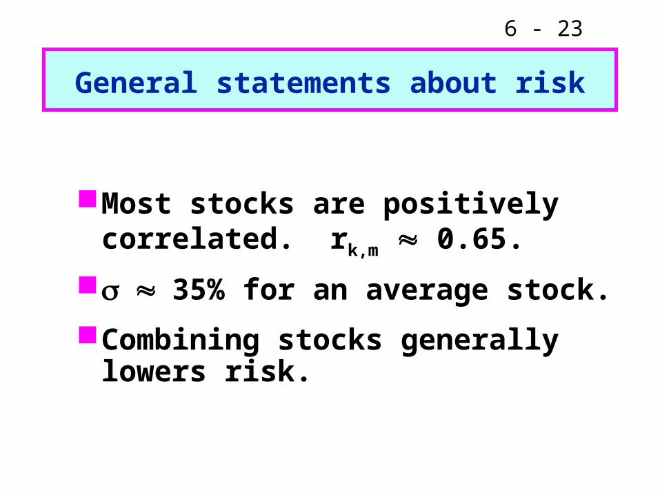
General statements about risk
Most stocks are positively correlated. rk,m 0.65.
35% for an average stock.
Combining stocks generally lowers risk.

6 - 24
Returns Distribution for Two Perfectly Negatively Correlated Stocks (r = -1.0) and
for Portfolio WM
25
15
0
-10 -10 -10
0 0
15 15
25 25
Stock W Stock M Portfolio WM
.. .
. .
.
.
..
.. . . . .

6 - 25
Returns Distributions for Two Perfectly Positively Correlated Stocks (r = +1.0) and
for Portfolio MM’
Stock M
0
15
25
-10
Stock M’
0
15
25
-10
Portfolio MM’
0
15
25
-10

6 - 26
What would happen to theriskiness of an average 1-stock
portfolio as more randomlyselected stocks were added?
p would decrease because the added
stocks would not be perfectly correlated but kp would remain relatively constant.^
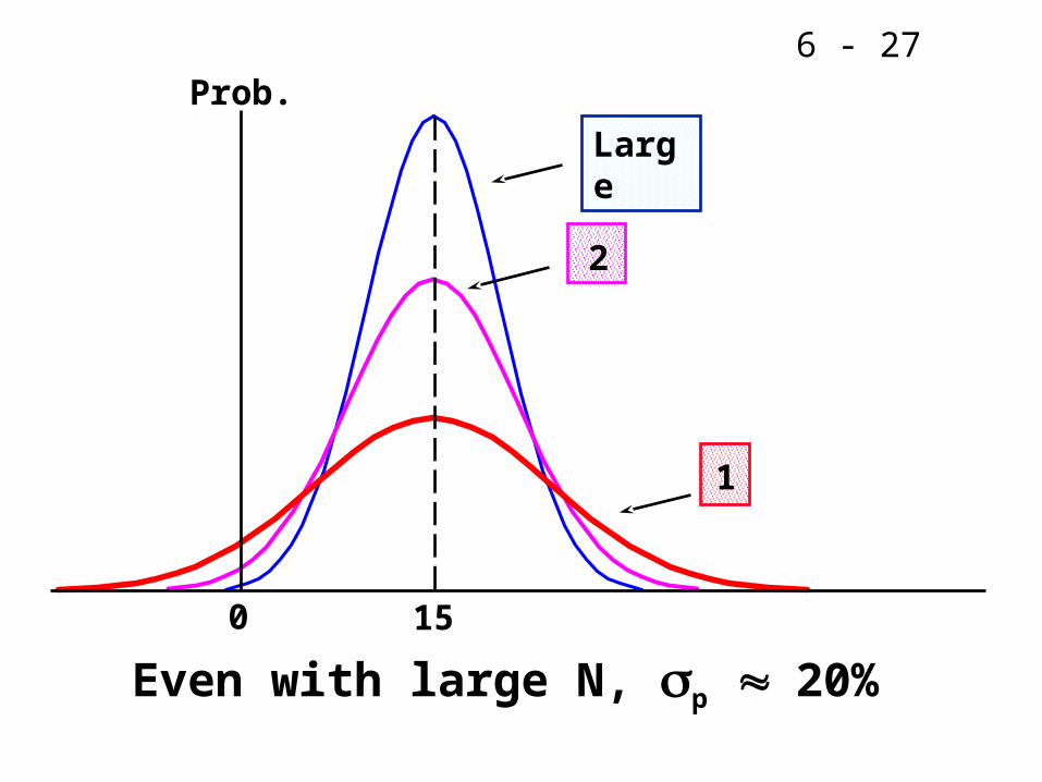
6 - 27
Large
0 15
Prob.
2
1
Even with large N, p 20%

6 - 28
# Stocks in Portfolio10 20 30 40 2,000+
Company Specific Risk
Market Risk
20
0
Stand-Alone Risk, p
p (%)
35

6 - 29
As more stocks are added, each new stock has a smaller risk-reducing impact.
p falls very slowly after about 10
stocks are included, and after 40 stocks, there is little, if any, effect. The lower limit for p is about 20%
= M .
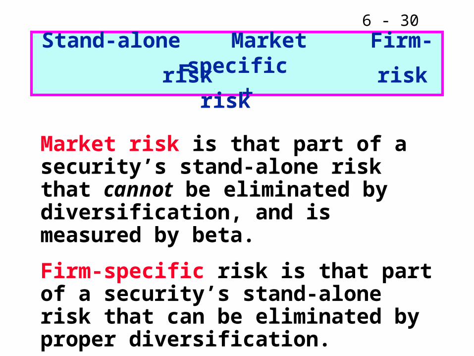
6 - 30
Stand-alone Market Firm-specific
Market risk is that part of a security’s stand-alone risk that cannot be eliminated by diversification, and is measured by beta.
Firm-specific risk is that part of a security’s stand-alone risk that can be eliminated by proper diversification.
risk risk risk= +
6 - 31
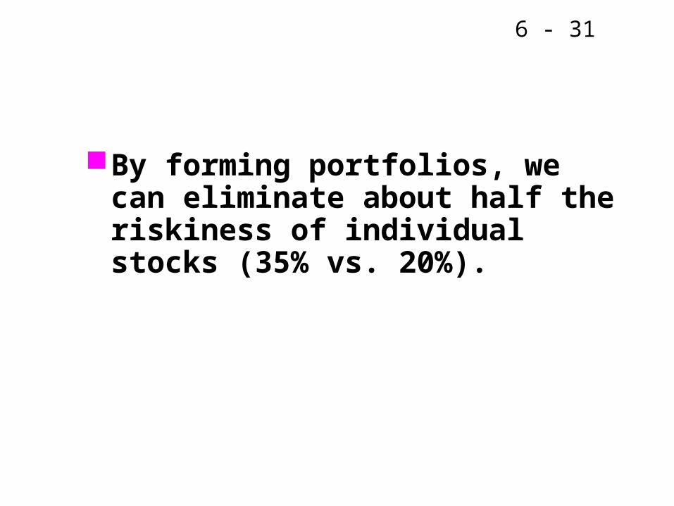
By forming portfolios, we can eliminate about half the riskiness of individual stocks (35% vs. 20%).
6 - 32
If you chose to hold a one-stock portfolio and thus are exposed to more risk than diversified investors, would you be compensated for all the risk you bear?
6 - 33
NO!
Stand-alone risk as measured by a stock’s or CV is not important to a well-diversified investor.
Rational, risk averse investors are concerned with p , which is based on market risk.

6 - 34
There can only be one price, hence market return, for a given security. Therefore, no compensation can be earned for the additional risk of a one-stock portfolio.
6 - 35
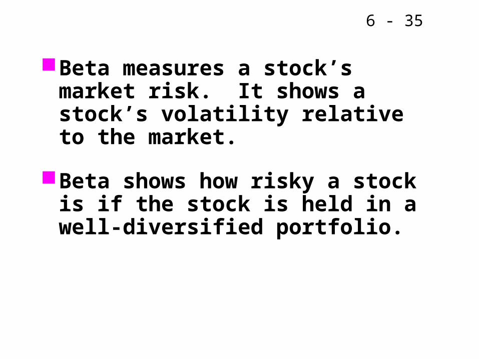
Beta measures a stock’s market risk. It shows a stock’s volatility relative to the market.
Beta shows how risky a stock is if the stock is held in a well-diversified portfolio.

6 - 36
How are betas calculated?
Run a regression of past returns on Stock i versus returns on the market. Returns = D/P + g.
The slope of the regression line is defined as the beta coefficient.
6 - 37
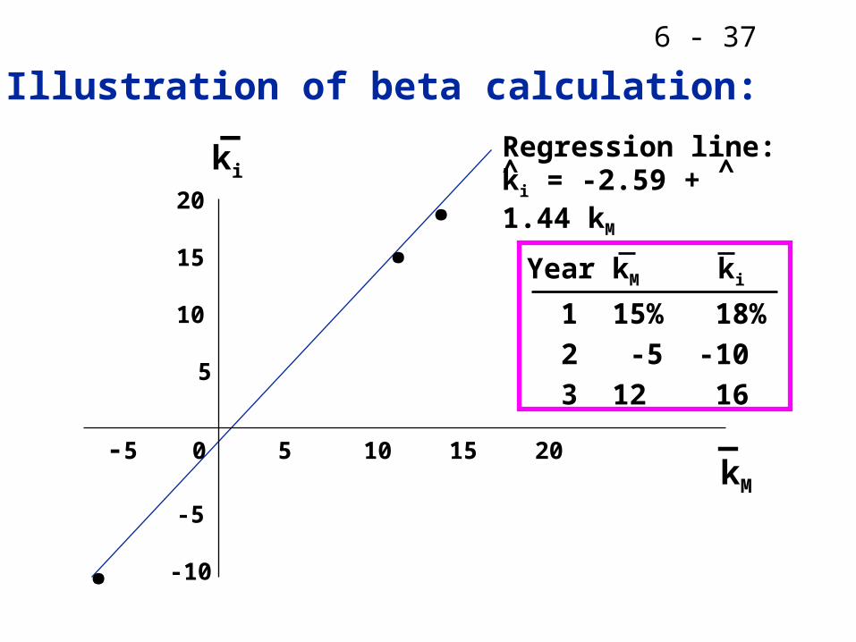
Year kM ki
1 15% 18%
2 -5 -10
3 12 16
.
.
.
ki
_
kM
_-5 0 5 10 15 20
20
15
10
5
-5
-10
Illustration of beta calculation:
Regression line:ki = -2.59 + 1.44 kM^ ^
6 - 38
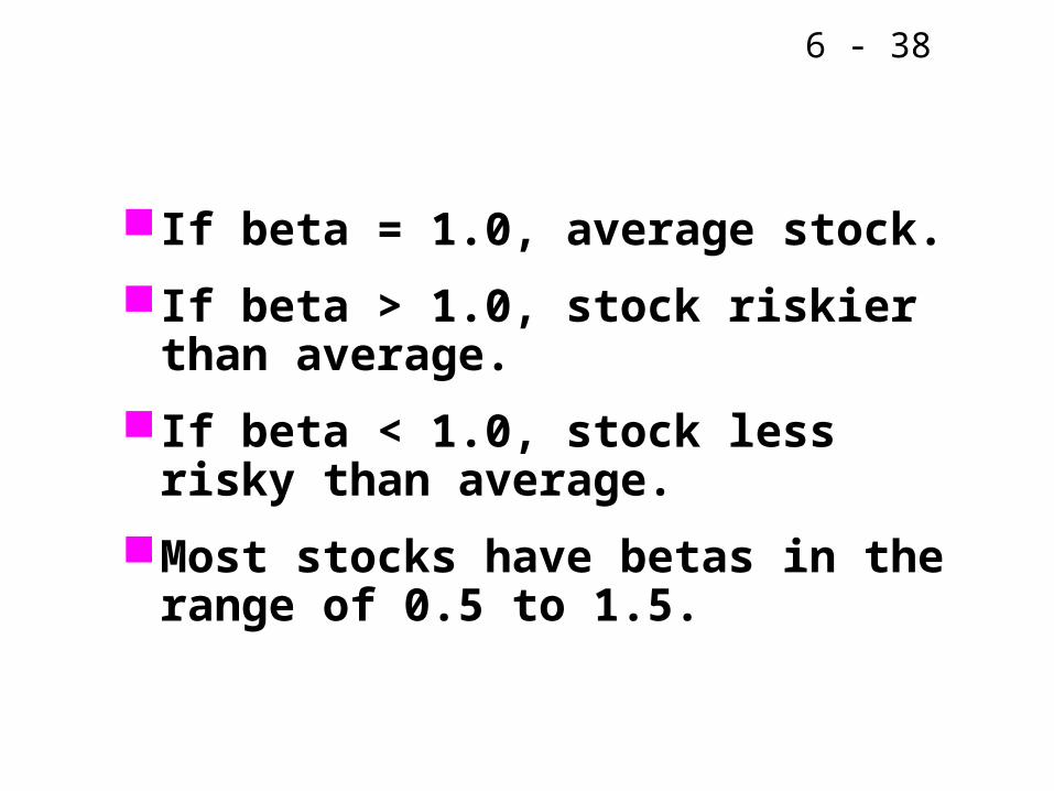
If beta = 1.0, average stock.
If beta > 1.0, stock riskier than average.
If beta < 1.0, stock less risky than average.
Most stocks have betas in the range of 0.5 to 1.5.

6 - 39
List of Beta Coefficients
Stock BetaMerrill Lynch 2.00America Online 1.70General Electric 1.20Microsoft Corp. 1.10Coca-Cola 1.05IBM 1.05Procter & Gamble 0.85Heinz 0.80Energen Corp. 0.80Empire District Electric 0.45
6 - 40
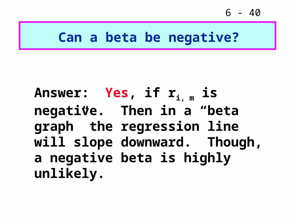
Can a beta be negative?
Answer: Yes, if ri, m is negative. Then in a “beta graph” the regression line will slope downward. Though, a negative beta is highly unlikely.
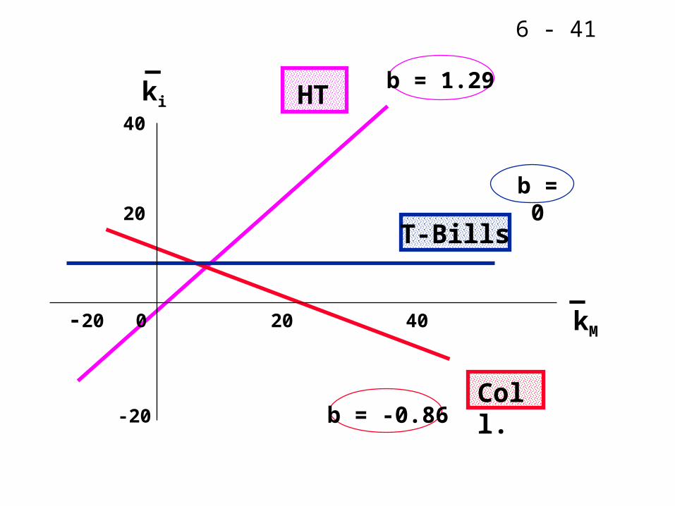
6 - 41
HT
T-Bills
b = 0
ki
_
kM
_-20 0 20 40
40
20
-20
b = 1.29
Coll.b = -0.86
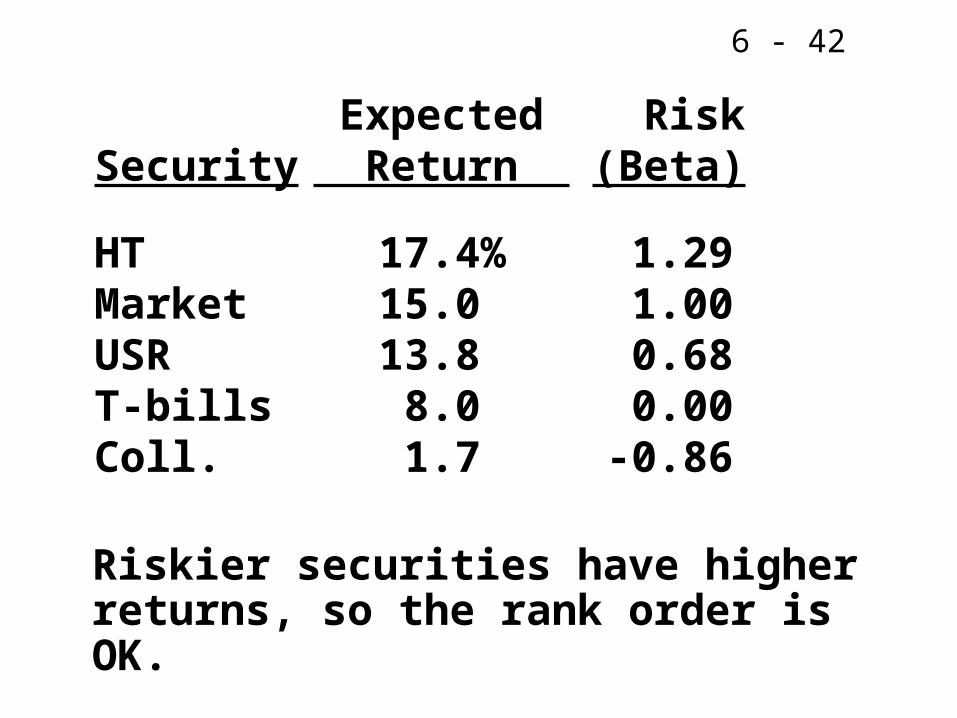
6 - 42
Riskier securities have higher returns, so the rank order is OK.
HT 17.4% 1.29Market 15.0 1.00USR 13.8 0.68T-bills 8.0 0.00Coll. 1.7 -0.86
Expected RiskSecurity Return (Beta)

6 - 43
Use the SML to calculate therequired returns.
Assume kRF = 8%.
Note that kM = kM is 15%. (Equil.)
RPM = kM – kRF = 15% – 8% = 7%.
SML: ki = kRF + (kM – kRF)bi .
^

6 - 44
Required Rates of Return
kHT = 8.0% + (15.0% – 8.0%)(1.29)= 8.0% + (7%)(1.29)= 8.0% + 9.0% = 17.0%.
kM = 8.0% + (7%)(1.00) = 15.0%.
kUSR = 8.0% + (7%)(0.68) = 12.8%.
kT-bill = 8.0% + (7%)(0.00) = 8.0%.
kColl = 8.0% + (7%)(-0.86) = 2.0%.

6 - 45
HT 17.4% 17.0% Undervalued: k > k
Market 15.0 15.0 Fairly valuedUSR 13.8 12.8 Undervalued:
k > kT-bills 8.0 8.0 Fairly valuedColl. 1.7 2.0 Overvalued:
k < k
Expected vs. Required Returns
^
^
^
^ k k

6 - 46
..Coll.
.HT
T-bills
.USR
SML
kM = 15
kRF = 8
-1 0 1 2
.
SML: ki = 8% + (15% – 8%) bi .
ki (%)
Risk, bi

6 - 47
Calculate beta for a portfolio with 50% HT and 50% Collections
bp= Weighted average = 0.5(bHT) + 0.5(bColl) = 0.5(1.29) + 0.5(-0.86) = 0.22.
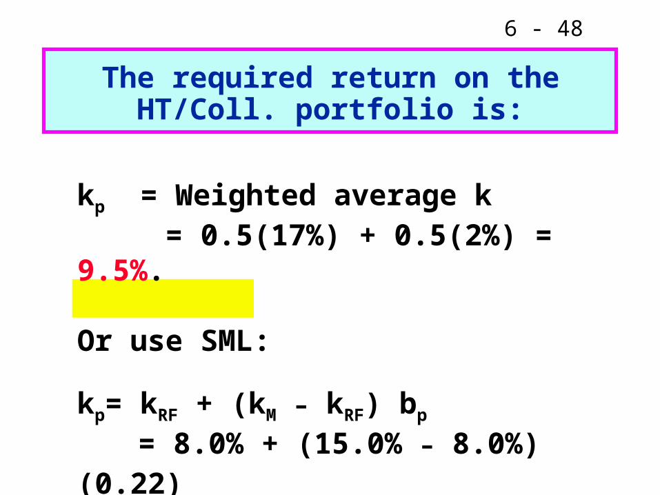
6 - 48
The required return on the HT/Coll. portfolio is:
kp = Weighted average k = 0.5(17%) + 0.5(2%) = 9.5%.
Or use SML:
kp= kRF + (kM – kRF) bp
= 8.0% + (15.0% – 8.0%)(0.22) = 8.0% + 7%(0.22) = 9.5%.

6 - 49
If investors raise inflation expectations by 3%, what would
happen to the SML?

6 - 50
SML1
Original situation
Required Rate of Return k (%)
SML2
0 0.5 1.0 1.5 Risk, bi
1815
11 8
New SML I = 3%

6 - 51
If inflation did not changebut risk aversion increasedenough to cause the marketrisk premium to increase by3 percentage points, whatwould happen to the SML?

6 - 52
kM = 18%
kM = 15%
SML1
Original situation
Required Rate of
Return (%)SML2
After increasein risk aversion
Risk, bi
18
15
8
1.0
RPM = 3%

6 - 53
Has the CAPM been verified through empirical tests?
Not completely. Those statistical tests have problems that make verification almost impossible.
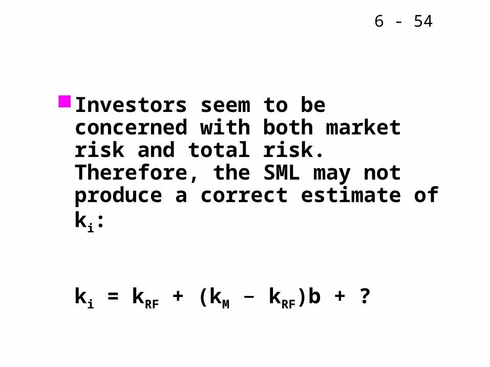
6 - 54
Investors seem to be concerned with both market risk and total risk. Therefore, the SML may not produce a correct estimate of ki:
ki = kRF + (kM – kRF)b + ?

6 - 55
Also, CAPM/SML concepts are based on expectations, yet betas are calculated using historical data. A company’s historical data may not reflect investors’ expectations about future riskiness.


