
A CORRELATION STUDY OF THE MAYS ROAD METER WITH THE SURFACE DYNAMICS PROFILOMETER
by
Roger S. Walker W. Ronald Hudson
Research Report Number 156-1
Surface Dynamics Road Profi1ometer Applications
Research Project 3-8-71-156
conducted for
The Texas Highway Department
in cooperation with the U. S. Department of Transportation
Federal Highway Administration
by the
CENTER FOR HIGHWAY RESEARCH
THE UNIVERSITY OF TEXAS AT AUSTIN
February 1973

The contents of this report reflect the views of the authors, who are responsible for the facts and the accuracy of the data presented herein. The contents do not necessarily reflect the official views or policies of the Federal Highway Administration. This report does not constitute a standard, specification, or regulation.
ii
-' -
PREFACE
This is the first report presenting results from Research Project 3-8-71-156,
"Surface Dynamics Road Profilometer Applications." The project was initiated
to carry out the implementation and operation of the Surface Dynamics (SO) Road
Profi1ometer in field and research applications.
The SO Profi1ometer measuring system was initially developed under Research
Project 3-8-63-73, '~eve10pment of a System for High-Speed Measurement of Pave
ment Roughness." A set of serviceability index (SI) prediction equations was
also developed during that project from the results of a large-scale rating
session of typical Texas pavements. The current project involved the imple
mentation of many of the research results from project 3-8-63-73. The assist
ance of Texas Highway Department Contact Representative Jim Brown is especially
appreciated. The assistance of project personnel Pat Macha1ek and Dennis Banks
should also be acknowledged.
February 1973
iii
Roger S. Walker W. Ronald Hudson
LIST OF REPORTS
Report No. 156-1, "A Correlation Study of the Mays Road Meter with the Surface Dynamics Profi1ometer," by Roger S. Walker and W. Ronald Hudson, discusses a study of the correlation between measurements made with the Mays Road Meter and the Surface Dynamics Profi1ometer and, based on this study, provides a set of calibration, operation, and control procedures for operation of the Mays Road Meter using serviceability index values from the profi1ometer as a measurement standard.
iv
\
ABSTRACT
A correlation study of roughness measurements obtained with the Mays Road
Meter (MRM) and the Surface Dynamics Profilometer (SDP) has been made and is
reported herein. In accordance with information obtained from this study, a
tentative set of calibration, operation, and control procedures has been de
veloped for the MRM to provide a means of obtaining roughness measurements for
Texas highways in terms of serviceability index. Several MRM's which have been
calibrated and for which the results have been reported according to these pro
cedures are currently in field use by the Texas Highway Department.
KEY WORDS: Surface Dynamics Profilometer, Mays Road Meter, serviceability index.
v
'.
SUMMARY
The problem of providing an objective tool for determining when a pavement
has failed has yet to be solved completely. However, development of the pave
ment serviceability performance concept by Carey and Irick during the AASHO
Road Test standardized a performance measurement procedure with which efforts
toward solving this problem might better be directed.
The Mays Road Meter (MRM) has been found to be an effective, inexpensive
device for measuring road roughness, but MRM roughness measurements are depend
ent on all factors which affect the mass and suspension system of the vehicle
used with the MRM and these factors vary from vehicle to vehicle. Therefore,
standard roughness measurement values are needed for calibration.
By use of the Surface Dynamics Profilometer (SOP) serviceability index
(SI) values as a standard, a correlation study of these two devices was made
and a general set of calibration, operation, and control procedures was developed
for MRM's purchased by the Texas Highway Department. The calibration, oper
ation, and control procedures-provide a means of reporting roughness in terms
of standard roughness values for all MRM's, thus enabling different devices to
give the same roughness readings for the same road section. Several MRM's have
been calibrated according to these procedures and are currently in use.
vi
IMPLEMENTATION STATEMENT
A general set of calibration, operation, and control procedures has been
developed for the Mays Road Meter (MRM) using the serviceability index values
from the Surface Dynamics Profilometer (SDP) as the measurement standard.
Several MRM's have been calibrated according to these procedures and are curw
rently being used in field operations. With these procedures, MRM's which are
purchased by the various THO districts can be used for riding quality measure
ments in terms of standard values.
vii
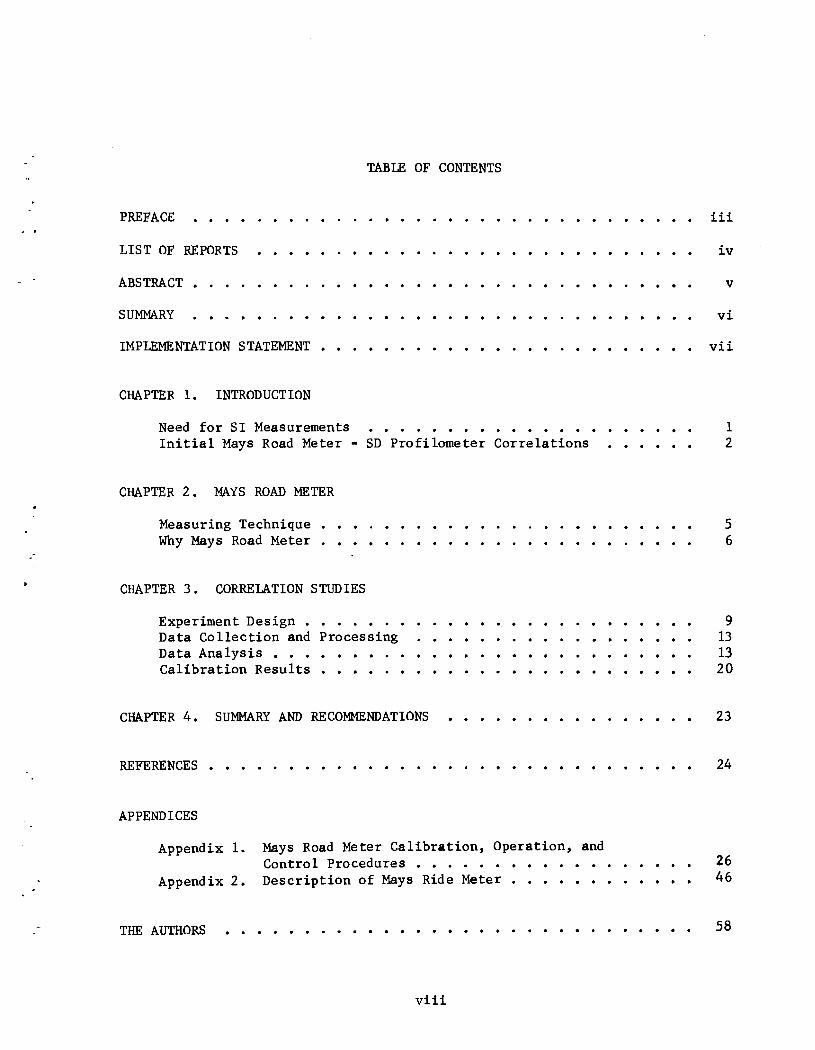
TABLE OF CONTENTS
PREFACE
LIST OF REPORTS
ABSTRACT
SUMMARY
IMPLEMENTATION STATEMENT
CHAPTER 1. INTRODUCTION
Need for S I Measurements ••••••••••••••• Initial Mays Road Meter - SD Profi1ometer Correlations
CHAPTER 2. MAYS ROAD METER
Measuring Technique Why Mays Road Meter
CHAPTER 3. CORRELATION STUDIES
Experiment Design • • . • • Data Collection and Processing Data Analysis • • . • Calibration Results • • • • • •
CHAPTER 4. SUMMARY AND RECOMMENDATIONS
iii
iv
v
vi
vii
1 2
5 6
9 13 13 20
23
REFERENCES • • • • • • • • • • • • • • • • . • • • • • • • • • • • • •• 24
APPENDICES
Appendix 1.
Appendix 2.
Mays Road Meter Calibration, Operation, and Control Procedures • • • Description of Mays Ride Meter • • • • • • •
26 46
TIlE AUTHORS •••••••••••••••••••••••.•••••• 58
viii
--
CHAPTER 1. INTRODUCTION
During the latter part of Project 3-8-63-73, '~evelopment of a System for
High-Speed Measurement of Pavement Roughness," a pilot study was conducted in
which roughness measurements of pavement sections obtained with the Mays Road
Meter (MRM) were compared with serviceability index (SI) values of the same
sections obtained with the Surface Dynamics Profilometer (SOP) (Ref 1). The
results of this study indicated that the roughness statistics obtained from
these two devices were highly correlated. Subsequent trials of the MRM pro
vided increased confidence in the use of this device for roughness measurements.
Consequently, one of the proposed tasks for Project 3-8-71-156 was to provide
a more extensive comparison between these devices and develop a procedure for
the calibration, operation, and control of the MRM using SI computations from
SOP data as the standard. This report summarizes the results of this task.
The Need for SI Measurements
The problem of determining when a pavement has failed has yet to be solved.
However, the development of the pavement serviceability performance concept by
Carey and Irick (Ref 2) during the planning of the AASHO Road Test was an at
tempt to standardize a performance measurement procedure with which efforts
toward solving this problem might better be directed. This concept was accepted
and used in research conducted by Project 3-8-63-73, and a set of SI prediction
equations or models was developed around slope variance computations of road
profile data obtained with the SOP (Refs 1 and 3). By using such models, a
standardized performance measurement procedure for Texas highways was established.
The resulting values are useful inputs to many different projects, such as
determining maintenance schedules and studying the effects of various environ
mental conditions on pavement.
The SOP has proven to be a good device for obtaining accurate road profile
information. However, because of its high equipment investment and operating
cost and the desirability of having a simple economical device available, it
was decided to investigate the Mays Road Meter (MRM). This device, however,
1
.-
2
unlike the SDP, is extremely sensitive to the vehicle in which it is installed
as well as to environmental and other conditions. Therefore, to be useful for
providing roughness measurements, these devices have to be calibrated to some
standard and then continually controlled to insure accuracy. The SDP is a
standard measuring device which can be used for calibration but a well-defined
procedure for checking the MRM is needed. Such a calibration procedure is de
scribed herein.
Initial Mays Road Meter - SD Profi1ometer Correlations
In the initial MRM-SDP correlation study, a 1969 Ford was used to house
the MRM device (Ref 1). An experiment was conducted in which two sets of
repeat runs over 15 test sections were made with the MRM. The average of the
two roughness measurements of each section (in inches per mile) was then cor
related with the SI values obtained for these same sections with the SDP. In
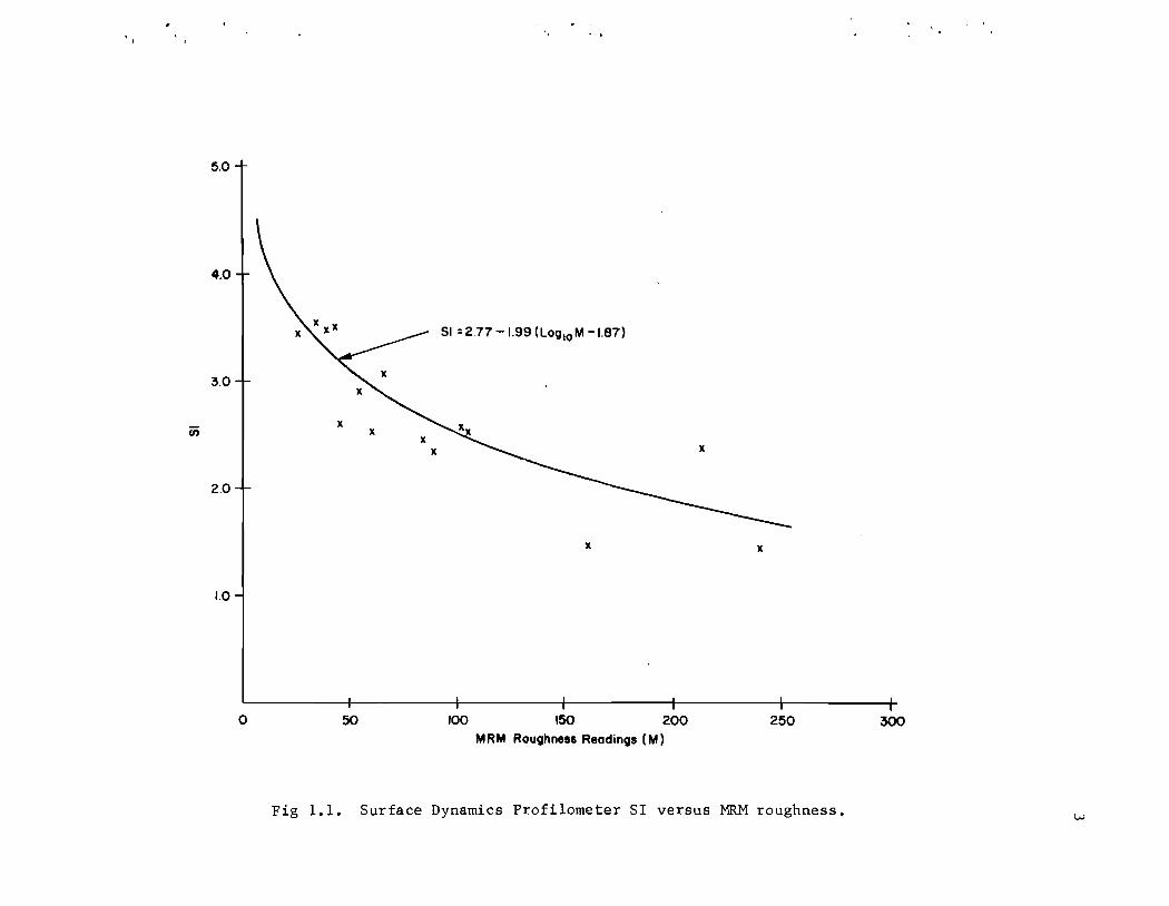
these comparisons, SI was regressed on the log MRM roughness readings, and
Eq 1.1 was obtained:
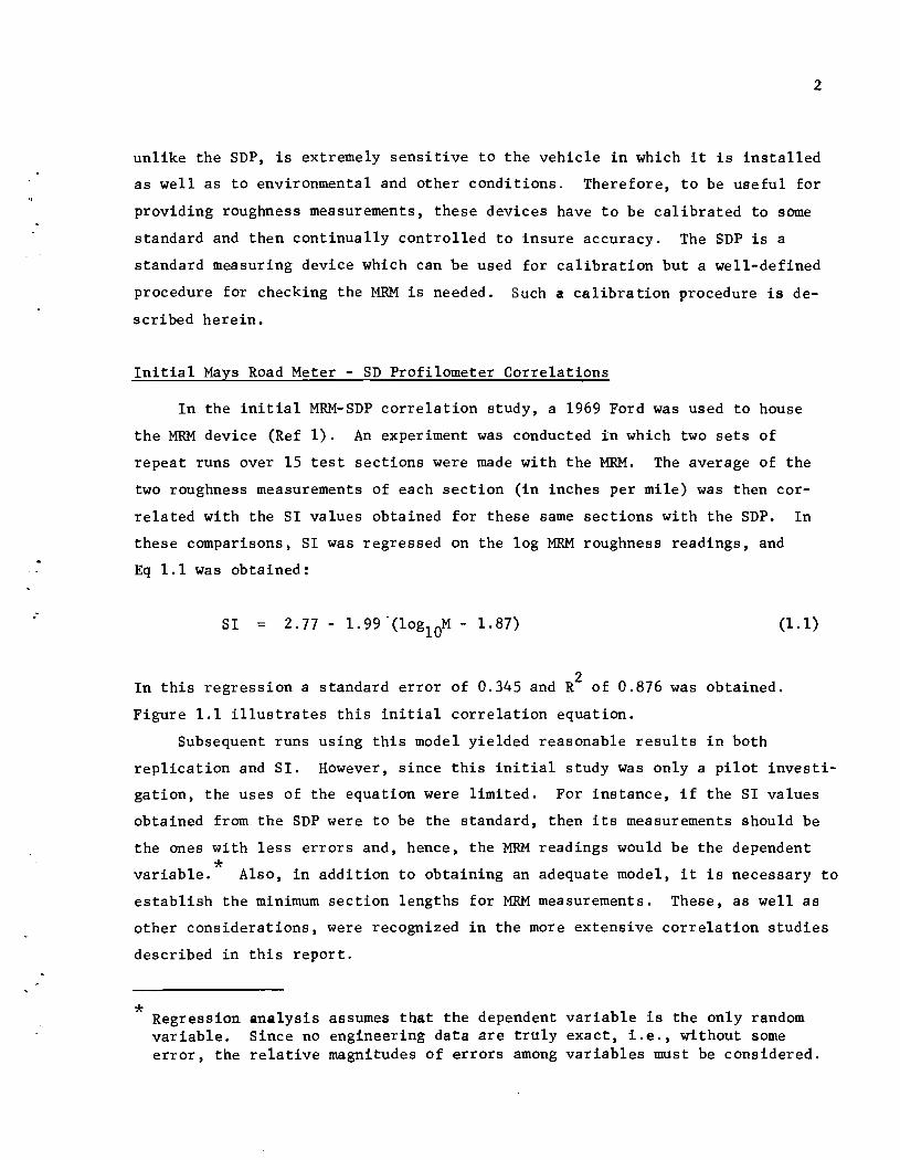
SI 2.77 - 1.99'(log10M - 1.87) (1.1)
2 In this regression a standard error of 0.345 and R of 0.876 was obtained.
Figure 1.1 illustrates this initial correlation equation.
Subsequent runs using this model yielded reasonable results in both
replication and SI. However, since this initial study was only a pilot investi-
ga tion, the uses of the equa tion were limited. For instance, if the SI values
obtained from the SDP were to be the standard, then its measurements should be
the ones with less errors and, hence, the MRM readings would be the dependent
* variable. Also, in addition to obtaining an adequate model, it is necessary to
establish the minimum section lengths for MRM measurements. These, as well as
other considerations, were recognized in the more extensive correlation studies
described in this report.
* Regression analysis assumes that the dependent variable is the only random variable. Since no engineering data are truly exact, i.e., without some error, the relative magnitudes of errors among variables must be considered.
5.0
4.0
SI =277-1.99(Log1o M-1.87)
3.0
u; x x x
x x
2.0
x x
1.0
o 50 100 150 200 250 300 M RM Roughness Readings (M)
Fig 1.1. Surface Dynamics Profilometer SI versus MRM roughness. w

:
4
The following chapter provides a brief description of the MRM device.
Chapter 3 presents details on the experiment and results. Appendix 1 provides
tentative calibration, operation, and control procedures for using the MRM
to obtain S1. These procedures are written so that they can be extracted for
MRM field use. Appendix 2 provides details on the Mays Ride Meter manufactured
by Rainhart Engineering.

CRAPI'ER 2. MAYS ROAD METER
The Mays Road Meter CMRM) was initially developed in 1967 by Ivan Mays,
a Texas Highway Department Senior Design Engineer, to provide a simple and
operationally useful device for measuring road roughness. Texas Transportation
Institute, Texas A&M University (Ref 4), subsequently confirmed the usefulness
of this device as a roughness measuring instrument. In fact, when compared
with the BPR Roughometer, the PCA Roadmeter, and the CHLOE Profi1ometer, the
MRM was recommended as the most appropriate of these devices for general field
use. The Louisiana Highway Department (Ref 5) also evaluated the MRM and
found it preferable to other existing roughness measuring devices. The primary
advantages of the MRM have appeared to be its ease of operation and the rough
ness record provided concomitantly with the roughness measurements, which gives
a permanent record of the locations of particular rough areas in a pavement.
It is not the purposes of this report to evaluate or compare the MRM with other
roughness measuring devices, ·but to correlate measurements with this device
with the serviceability index values of the SDP. However, following a brief
discussion of the general operating characteristics of the MRM, the reasons
for selecting the MRM for this study are indicated.
Measuring Technigue
The general measuring technique of the MRM is similar to that of the BPR
and PCA devices. That is, roughness measurements are proportional to the
vertical changes between the vehicle body and its rear axle as the vehicle
travels over a pavement. These vertical motions are accumulated and are
recorded on an advancing paper tape or strip chart by a recording pen simulta
neously moving at a rate proportional to the movements of the vehicle body and
its differential. Vehicle distance traveled is also indicated on the roughness
chart by an automatic event marker connected to the speedometer drive system.
By measuring the amount of chart movement per unit of road length traveled,
a roughness measurement directly proportional to the total body-differential
5

movement, in inches per mile, can be obtained. The roughness pattern or
signature permanently recorded on the paper tape provides additional informa
tion for indicating where particular rough areas were. Thus, in addition to
a roughness number or index value, the proportion the various pavement areas
contribute to the overall roughness measurement is also provided. (This par
ticular characteristic was quite useful in obtaining minimum measurement dis
tances for SI computations. See the experiment design details of Chapter 3.)
The appendix provides complete details of the measuring technique.
6
The initial MRM instrument employed mechanical pulleys for driving the
paper chart tape and for the pen arm movements. Rainhart Engineering Company
is currently manufacturing a commercial version of the device (called the Mays
Ride Meter) and has replaced the pulleys with a photocell sensing system,
which drives a stepping motor for pen and chart drive movements. The Rainhart
version is operationally much more convenient and has been found to be more
accurate. The recording device of the Rainhart version, for instance, can be
placed in the operator's lap and additional notes can be transcribed on the
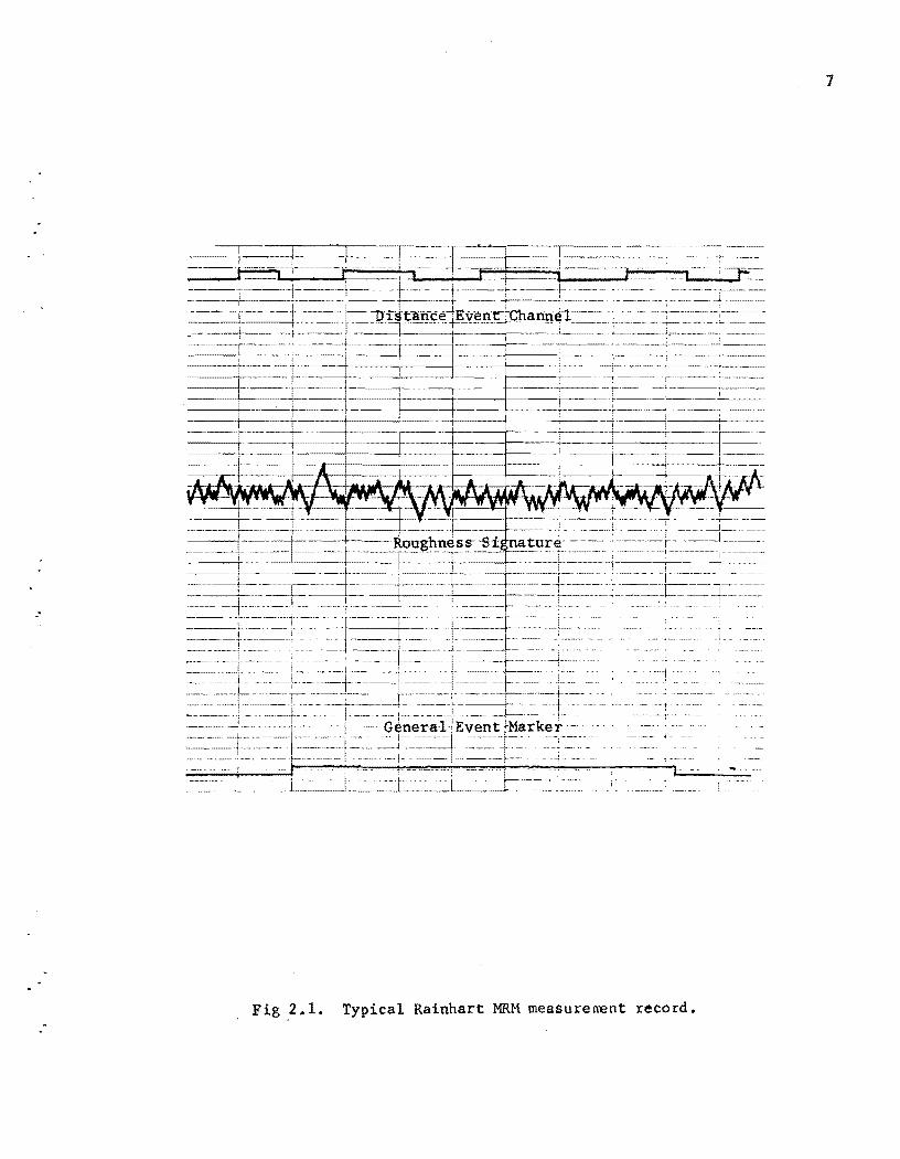
chart paper while the machine is in operation. Figure 2.1 depicts a typical
paper tape measurement recorq of the Rainhart MRM. As noted in this figure,
for this device 1/20-mile distance markers provide the distance reference for
the roughness measurements. An additional event marker is supplied for further
record identification.
Why Mays Road Meter
The need for an immediate SI measurement has been detailed in Refs 1 and
6. The MRM was available, and because of its favorable characteristics, as
indicated in a Texas Transportation Institute (TTl) study, it was selected
for a pilot correlation study, as earlier indicated.
Probably the only other instruments which would compare economically with
the MRM are the PCA and BPR devices. All three measure roughness indirectly
by measuring vehicle body motion, and are obviously correlated for the typical
road section with slope variance, roughness index, profile wavelengths, vehicle
shock absorbers, vehicle type, body weight, etc. None measures roughness
characteristics directly. The PeA meter, which is sometimes incorrectly
termed a slope variance measuring device, does provide an estimate of slope
variance by correlation equations, but it obviously does not measure slope
variance directly. This fact is easily demonstrated by measuring an imaginary
7
.'
Fig .2.1. Typical Rainhart MRM measurement record.
road which has a profile in the form of a sine wave with a period that is an
integer multiple of the base length used in the slope variance calculation.
For such a road, the slope variance is, of course, identically zero; however,
there will be body motion of the car if the amplitude of the wave is great
enough.
8
All the devices examined are considered equally undesirable for accurate
roughness measurements in comparison with the SDP. The MRM, however, was
found to be the most convenient and hence was selected. The following chapter
provides details on the SDP-SI and MRM measurements correlation study.
--
CHAPTER 3. CORRELATION STUDIES
As indicated in Chapter 1, a pilot study comparing SDP-SI values with
MRM roughness measurements revealed certain similarities between these two
devices. Because of this initial study, the need for extensive SI measurements
on Texas pavements, and the MRM cost and operational advantages, it was decided
to more completely investigate the correlation between these two devices. Once
an acceptable correlation model could be found, then a general procedure for
* calibrating MRM devices to the SDP-SI measurements could be developed. This
chapter provides the description and results of the model development phase of
this study. The calibration procedure described in Appendix 1 uses this same
experimental design in obtaining the SDP-MRM calibration model. The SI models
used for the correlations are direct functions of road profile wave amplitudes
rather than slope variance, patching and cracking, etc. Initially, the slope
variance models were employed in the experiment; however, as the experiment
progressed, a new SI prediction equation was developed which predicted SI
entirely as a function of road profile wave amplitudes. Details of this model
will be provided in the final report on Research Project 156.
Experiment Design
*
The primary function of the experiment design is to
(1) determine an adequate correlation model which can be used for predicting SI for the MRM; and
(2) given this model, determine the general operational requirements of the model, such as minimum section length and replication.
In order to prevent confusion, the differences between the terms correlation and calibration will be given for this report. Correlation consists of determining how well MRM values can be related to SDP-SI values. The equation which relates these two variables is referred to as the correlation equation or correlation model. Calibration is the process of correlating each specific MRM in accordance with this correlation model.
9

10
For the experiment, both the old mechanical type MRM built by the Texas
Highway Department and the electronic controlled Rainhart manufactured device
were used. Initial studies were to include only the former; however, during
the study, Project 1-8-69-123, '~ System Analysis of Pavement Design and Re
search Implementation," purchased a Rainhart manufactured meter and it was
included in the experiment in order to increase the sample size for statistical
. * purposes and to provide Project 123 with a calibrated MRM for project work.
The study results are primarily oriented toward the Rainhart MRM, since, first,
it appears to have both an accuracy and operational advantage over the mechani
cal device, and, second, it is commercially manufactured and hence is likely
to receive more widespread usage than the other meter.
Both devices provide distance events at 1/20-mi1e resolution; thus,
replication and/or minimum distance requirements will be integer multiples
of these 1/20-mi1e events. With this resolution stipulation, the following
experiment was designed.
Twenty-three 1/4-mi1e test sections considered representative of the pave
ment roughness range for .Texas pavements were selected. Another criterion for
selection was that each section have relatively homogeneous roughness character-** istics throughout the 1/4-mi1e test section. Four replication runs were made
with the MRM over each section; the sections were also measured with the SDP
and their respective SI values were computed. Because of the requirement of
item 2 above, to determine minimum section length and replication requirements,
each MRM section run was divided into five 1/20-mi1e segments, thus providing
a total of 20 sample segments per section. The overall experimental design is
illustrated in the flow chart of Fig 3.1. The section segmenting is indicated
by item 1 of this figure. Assuming any single segment provides an unbiased
estimate of the SI (because of the assumed homogeneous roughness characteristic
* Since the initial correlation experiment, several additional MRM's (Rainhart version) have been calibrated according to the procedures specified in this chapter.
**The relatively homogeneous roughness was judged in the same manner as in the original S1 rating session of Ref 3, i.e., it had to be constant from the standpoint of typical pavement characteristics.

(1)
(2)
(3)
-' _(i,n M) 5 SI = 5e ~
(4)
(5) No
41 = I - 11
(6)
11
~/ '.
Separate test section into five 1/20-mi1e segments. Make four repeat runs. ~~~~
jth section (j = 1.2,3 .•• ,23)
Randomly generate from segment samples 20 sample distance sets for each section.
.th . J sect10n
Ou ,
D LJ ,
20 sample distance sets for jth section
Using 20th sample set (1 mile), find suitable SI20 ~ F(M1o) where M = one mile roughness measurement (inches per mile).
. Ir
Compute SI = F(~) for ith sample set = i/2~ mile.
'. Does SIi differ significantly from SI20 in ~ or exhibit poor correlation or exhibit lack of fit?
Yes
Select minimum roughness measurement distance as I/20-mi1e.
Fig 3.1. MRM-SDP correlation experiment.
12
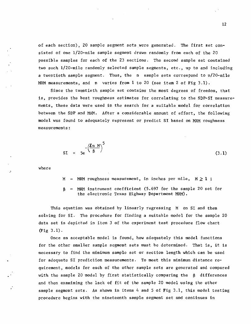
of each section), 20 sample segment sets were generated. The first set con
sisted of one 1/20-mi1e sample segment drawn randomly from each of the 20
possible samples for each of the 23 sections. The second sample set contained
two such 1/20-mi1e randomly selected sample segments, etc., up to and including
a twentieth sample segment. Thus, the n sample sets correspond to n/20-mi1e
MRM measurements, and n varies from 1 to 20 (see item 2 of Fig 3.1).
Since the twentieth sample set contains the most degrees of freedom, that
is, provides the best roughness estimates for correlating to the SDP-S1 measure
ments, these data were used in the search for a suitable model for correlation
between the SOP and MRM. After a considerable amount of effort, the following
model was found to adequately represent or predict SI based on MRM roughness
measurements:
where
SI (3.1)
M MRM roughness measurement, in inches per mile, M ~ 1 ;
~ = MRM instrument coefficient (5.697 for the sample 20 set for the electronic Texas Highway Department MRM).
This equation was obtained by linearly regressing M on SI and then
solving for SI. The procedure for finding a suitable model for the sample 20
data set is depicted in item 3 of the experiment test procedure flow chart
(Fig 3.1).
Once an acceptable model is found, how adequately this model functions
for the other smaller sample segment sets must be determined. That is, it is
necessary to find the minimum sample set or section length which can be used
for adequate SI prediction measurements. To meet this minimum distance re
quirement, models for each of the other sample sets are generated and compared
with the sample 20 model by first statistically comparing the ~ differences
and then examining the lack of fit of the sample 20 model using the other
sample segment sets. As shown in items 4 and 5 of Fig 3.1, this model testing
procedure begins with the nineteenth sample segment set and continues in
13
decreasing distance order until a model is found which is significantly
different or inadequate. The sample segment set at which this occurs thus
represents the minimum required MRM segment distance and furthermore, since
these segments are randomly selected, it also indicates the replication re
quirements. For example, it was found that the mechanical MRM should include
at least three 1/20-mile distance segments for adequate SI predictions. This
means that either a 1/20-mile section length must be run three times and the
sum of these three measurements used, or a 3/20-mile section can be used, which
requires only one run.
Data Collection and Processing. As indicated in Fig 3.1, the data collec
tion phase involved running both the MRM and SDP over 23 test sections and
obtaining the appropriate roughness measurements for each section. The MRM
data runs consisted of four replicate runs, as discussed earlier. The roughness
measurements were taken directly from the MRM roughness records. The SI values
for each SDP profile run, however, could not be computed until the profile data
were digitized and the power or variance spectrum computed. The SI values were
then computed directly from the power or variance spectral estimates after they
were transformed to wave amplitudes.
A typical MRM roughness record (Fig 2.1) provides three information chan
nels, a distance marker (indicating 1/20-mile distance traveled increments),
a vehicle body deflection measurement, and a general event marker used by the
operator for signaling certain measuring events; such as the start or end of
a particular test section. For the twenty 1/20-mile sections for each 1/4-mile
section, each 1/20-mile distance mark is measured in inches and recorded from
the first channel of the roughness record. The distance measurements may then
be converted to actual vehicle body deflection measurements per one-mile sec
tion by multiplying each by 20 times the MRM measurement vehicle differential
ratio (6.4 for the Rainhart manufactured device).
Data Analysis
The data analysis phase consists of finding an adequate SI model for the
twentieth sample segment and then determining the model's minimum section
length constraint. Since regression analysis would be used for obtaining this
model and the dependent variable is to be the MRM roughness measurement (i.e.,
the greatest errors are assumed to exist in the MRM roughness readings, or

.-
14
the SDP-S1 computations are more stable), the MRM readings were then examined
for homogeneous variance characteristics. Plots of the coefficient of varia
tion of the MRM roughness readings revealed a somewhat constant relationship
for the different roughness readings. Such a relationship suggests the use
of the log transformation on this variable (see Ref 7), in order to insure
the homogeneous roughness assumptions in the regression analysis.
As indicated in the previous section, the search for a suitable model to
show correlation between the SDP and MRM involved using the data from the
twentieth sample set, since this set provided the best roughness estimates
(i.e., it contained 20 independent roughness estimates). The following linear
regression is then performed for the following model.
y \3X + € (3.2)
where
y in M . ,
~ = linear regression coefficient;
M Mays Road Meter accumulated roughness reading, in inches per mile;
X [In(sIS1) ] liS
€ the residual or regression error.
The Y intercept ~o is zero for this model since the SI is five, the
* MRM roughness value is at its minimum, which is to be assumed one.
Equation 3.1 can be obtained from Eq 3.2 by solving for SI in terms of
M. Figure 3.2 provides a plot of the sample 20 data set using the sample
20 model.
* Since M typically will always be greater than one, it was assumed that the mlnlmum M is one rather than zero. The 81 of five is a boundary condition and is typically never reached; thus, the selection of one rather than zero is used primarily for convenience.

.-
o CO •
15
95 PERCENT CONFIDENCE INTERVAL
0r-------====~~~~--__ CD •
o o •
o N •
..... 0 (f)~
• N
o co • -
o CD •
o
o
)(
a;-------~--------r_------~------_,--------T_------_r----·0.00 1.00 2.00 3.00 4.00 5.00 e.oo
LN(MRMl Fig 3.2. SDP-S1 values versus log Mays road roughness readings.
.-
As discussed in the experimental design section, the adequacy of the
sample 20 model for the smaller sample segment sets establishes the minimum
MRM resolution constraints. To meet this minimum distance requirement, the
following tests were performed on each sample segment model as indicated in
items 4 and 5 of Fig 3.1.
16
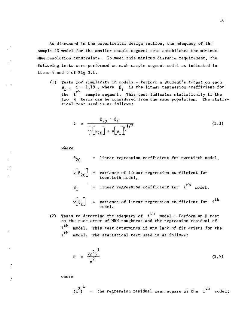
(1) Tests for similarity in models - Perform a Student's t-test on each ~i' i = 1,19 , where ~i is the linear regression coefficient for
the ith sample segment. This test indicates statistically if the two ~ terms can be considered from the same population. The statistical test used is as follows:
t
where
~20
(3.3)
linear regression coefficient for twentieth model,
variance of linear regression coefficient for twentieth model,
linear regression coefficient for th i model,
variance of linear regression coefficient for model.
.th 1
(2) Tests to determine the adequacy of ith model - Perform an F-test on the pure error of MRM roughness and the regression residual of
ith model. This test determines if any lack of fit exists for the
ith model. The statistical test used is as follows:
F (3.4 )
where
the regression residual mean square of the .th 1 model;
17
2 a the pure error variance.
Table 3.1 provides the results of these tests for the Rainhart MRM used
in Project 123. As noted from this table, the sample 20 model for the Rainhart
device can be used without significant error down to 1/20 of a mile resolution.
However, it was found that the THD device should be used on sections of no less
than 0.2-mile total length. As a further precaution and for consistency in the
calibration procedures of Chapter 4, it is recommended that neither device be
used on sections of less than 0.2-mile unless replication is provided.
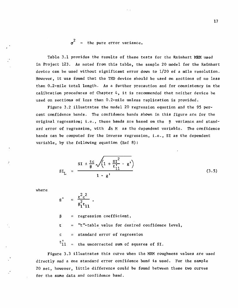
Figure 3.2 illustrates the model 20 regression equation and the 95 per
cent confidence bands. The confidence bands shown in this figure are for the
original regression; i.e., these bands are based on the S variance and stand
ard error of regression, with in M as the dependent variable. The confidence
bands can be computed for the inverse regression, i.e., sr as the dependent
variable, by the following equation (Ref 8):
s r ± g )(1 + s; 2 - g')
~ tll (3.5)
1 - g'
where
g'
regression coefficient,
t "til-table value for desired confidence level,
standard error of regression
the uncorrected sum of squares of sr.
Figure 3.3 illustrates this curve when the MRM roughness values are used
directly and a one standard error confidence band is used. For the sample
20 set, however, little difference could be found between these two curves
for the same data and confidence band.

18
TABLE 3.1. MODEL TESTS FOR ACCEPTABILITY
Test on !3 i' Test for Lack Sample Set II t"- Value of Fit, I'F "-Value
1 -1.044 1.150
2 0.298 1.189
3 -0.354 0.853
4 -0.155 0.977
5 0.366 0.933
6 -0.194 0.920
7 0.058 0.884
8 0.144 1.193
9 0.269 0.885
10 -0.235 1.045
11 -0.345 0.901
12 0.090 0.866
13 -0.103 0.919
14 -0.012 0.865
15 -0.284 1.155
16 -0.198 1.055
17 -0.105 0.827
18 -0.023 1.024
19 -0.070 0.916
20 0.855

I--!
u:
.-
0 Cf)
'>t-
C) 0
'>t-
0 r-J
(Y")
0 '>t
C-J
o en
o o
~
MRYS MFTER VS S1
\
80,GO 160.GO 240.GO 320.00
MRM (INCHES)
I 400.00
19
Fig 3.3. Confidence bands for inverse regression for the correlation model.

:
It is actually more expedient to examine the average error between the
predicted and actual 81 values. These errors are provided for five separate
MRM's calibrated according to this model in the following section.
Calibration Results
20
As previously noted, the procedures described in this chapter have been
used to develop a correlation model which would be useful in calibrating MRM
devices. Five MRM's have been calibrated according to these procedures. The
results of these calibrations are summarized in Table 3.2. Four of the devices
were manufactured by Rainhart Company. The fifth is the older model THO me
chanical device.
All but the device used by TTl were calibrated according to Eq 3.1. A
small variation in this equation was used for the TTl calibration model in
order to get a better fit. The difference could have been due to the leaf
suspension system of the vehicle in which the TTl MRM instrument was mounted.
In fact, it has been recommended that the MRM be operated only in a coil-spring
type suspension system. Even so, with the model of Eq 3.1, there actually was
no statistically significant" lack of fit, primarily due to the larger replica
tion error of the TTl device, as illustrated in Table 3.2. By examining a
plot of 81 versus the MRM roughness readings similar to Fig 3.2 for this de
vice, it was observed that a better fit could be obtained by using an equation
of the form
81 (3.6)
This different model could be due to the different suspension system, as
noted, or perhaps two parameters are required by the general calibration model.
The appropriate general model will become more apparent only as more MRM de
vices are calibrated (see the note on page 22).
The Rainhart device belongs to Rainhart Company and was calibrated prima
rily for research reasons to see if this general curve worked well on their
instrument, which was mounted in a 1963 Chevrolet stationwagon. As noted,
an acceptable calibration (or, for this case, correlation) resulted.

."
21
TABLE 3.2. CALIBRATION RESULTS
* ** Replication SI Model R2 Device Error Error
File D-8 0.252 5.697 0.319 0.998
District 21 0.234 5.633 0.342 0.998
*** TTl 0.424 5.192 0.292 0.994
Rainhart 0.257 5.267 0.351 0.997
Inhouse MRM 0.353 5.532 0.473 0.996
* Replication of pure error (log M, in inches per mile) used for testing lack of fit in the regression equation, Eq 3.2.
** Standard error between actual and predicted SI from Eq 3.1.
*** The model used varied from Eq 3.1 in the exponential term (see text).
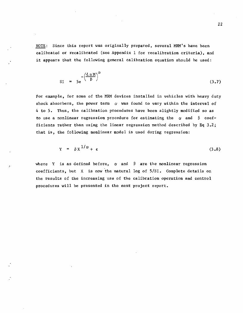
NOTE: Since this report was originally prepared, several MRM's have been
calibrated or recalibrated (see Appendix 1 for recalibration criteria), and
it appears that the following general calibration equation should be used:
22
SI = (3.7)
For example, for some of the MRM devices installed in vehicles with heavy duty
shock absorbers, the power term a was found to vary within the interval of
4 to 5. Thus, the calibration procedures have been slightly modified so as
to use a nonlinear regression procedure for estimating the a and ~ coef
ficients rather than using the linear regression method described by Eq 3.2;
that is, the following nonlinear model is used during regression:
Y = ~ X 1/ a + e: (3.8)
where Y is as defined before, a and ~ are the nonlinear regression
coefficients, but X is now the natural log of S/SI. Complete details on
the results of the increasing use of the calibration operation and control
procedures will be presented in the next project report.

CHAFfER 4. SUMMARY AND RECOMMENDATIONS
A correlation study of roughness measurements obtained with the Surface
Dynamics Profi1ometer (SDP) and the Mays Road Meter ~) has been made.
Based on results of this study, a set of calibration, operation, and control
procedures has been developed for the MRM in order to provide a means of ob
taining standard roughness measurements for Texas highways in terms of service
ability index (SI). These procedures involve correlating the MRM roughness
readings, in inches per mile, with SI values based on SDP readings. Because
of the SDP measurement characteristics, SI values computed from road profile
data obtained with this instrument provide an accurate measurement standard.
Several MRM devices have been calibrated according to these procedures
and are currently in use. Initial use of these procedures to obtain SI is
quite promising, and the standard roughness measurements for roads throughout
Texas which are provided are invaluable information to aid in solving the prob
lems of pavement failure.
Because of the encouraging results of the correlation study, the develop
ment of a tentative set of procedures for the calibration, operation, and con
trol of the MRM, and the use of these procedures in field operations, the
following recommendations are made.
(1) Additional MRM's should be purchased by the various Districts and calibrated and used by these Districts for obtaining numerous measurements of pavements for maintenance and other considerations.
(2) When a sufficient number of these devices are available, further experiments can be conducted to investigate the effects of temperature, weather, tire pressure, etc.
(3) As devices are purchased and used according to the calibration, operation, and control procedures, feedback should be provided to this project so that modifications to these procedures can be made on the basis of experience gained from extensive field use.
23

REFERENCES
1. Walker, Roger S., W. Ronald Hudson, and Freddy L. Roberts, '~eve1opment of a System for High-Speed Measurement of Pavement Roughness, Final Report," Research Report No. 73-5F, Center for Highway Research, The University of Texas at Austin, May 1971.
2. Carey, W. N., Jr., and P. E. Irick, 'The Pavement Serviceability-Performance Concept, II Bulletin 250, Highway Research Board, Washington, D. C., 1960.
3. Roberts, Freddy L., and W. Ronald Hudson, '~avement Serviceability Equations Using the Surface Dynamics Profi1ometer," Research Report No. 73-3, Center for Highway Research, The University of Texas at Austin, April 1970.
4. Phillips, M. B., and Gilbert Swift, '~Comparison of Four Roughness Measuring Systems," Research Report 32-10, Texas Transportation Institute, Texas A&M University, College Station, Texas, August 1968.
5. Law, S. M., and W. T. Burt, III, ''Road Roughness Correlation Study," Research Report No. 48, Louisiana Department of Highways, Research and Development Section, June 1970.
6. Walker, Roger S., Freddy L. Roberts, and W. Ronald Hudson, I~ Profile Measuring, Recording, and Processing System," Research Report No. 73-2, Center for Highway Research, The University of Texas at Austin, April 1970.
7. Bartlett, M. S., ''The Use of Transformations, II Biometrics, Vol 3, No. 39, 1947.
8. Williams, E. J., Regression Analysis, John Wiley and Sons, Inc., New York, New York, 1964, p 100.
9. Mays Ride Meter Booklet, Rainhart Co., Austin, Texas, 1972.
24

!!!!!!!!!!!!!!!!!!!"#$%!&'()!*)&+',)%!'-!$-.)-.$/-'++0!1+'-2!&'()!$-!.#)!/*$($-'+3!
44!5"6!7$1*'*0!8$($.$9'.$/-!")':!

APPENDIX 1. MAYS ROAD METER CALIBRATION, OPERATION, AND CONTROL PROCEDURES
This appendix provides a tentative set of procedures for the calibration,
operation, and control of the Mays Road Meter based on the findings in Chap-
ter 3. This appendix has been written so that it can be extracted without modi
fication for field use and can be made available to MRM field personnel who
are not interested in the model development and project details. There is,
therefore, some duplication of what is presented in other sections of this
report.
MRM roughness measurements are typically obtained in inches of vertical
vehicle motion per mile. Since these measurements are dependent on all factors
which affect a vehicle's suspension system, and because these factors vary
from vehicle to vehicle, a standard roughness value which can be used for all
instruments is needed. The procedures that are described herein provide such
a standard value unit. The standard value used, serviceability index (81), is a
single number ranging from zero to five, with five for a road or pavement con
sidered perfect and zero for one considered impassable. SI values are obtained
from inches-per-mile readings by use of a calibration table developed from a
calibration equation. The SI values simply provide a means of correlating the
roughness readings for the same section by two separate instruments.
The procedures described are divided into three areas: (1) calibration,
(2) operation, and (3) control. Calibration involves developing the necessary
tables for converting MRM roughness readings, in inches per mile, to 81 values.
The operation section indicates a standard method for measuring roughness. The
control section is a method of insuring that the MRM is functioning properly.
It should be noted that the control procedures described are for MRM devices
in general. It should also be noted that no measuring device ever gives exactly
the same measurement each time; that is, there are measurement errors. These
errors can be divided into two types: actual MRM measurement errors (equip
ment errors) and errors due to the non-homogeneous roughness characteristics
of roads.
26

:
27
Calibration
MRM calibration includes running roughness measurements on 25, 1/4-mi1e
long pavement sections, which initially are located in the Austin area, and
developing the tables necessary to convert MRM roughness readings to SI values.
The measurements must be made in accordance with the following specifications:
(1) MRM vehicle - The MRM must be calibrated in the vehicle in which it is to operate. Any physical characteristic (such as vehicle weight and shock absorbers) which affects vehicle body motion should be the same during calibration as in operation.
(2) Calibration sections - The 25 calibration sections have been marked by white paint stripes at the beginning and end of each test section. For scheduled calibration runs, two red flags on the right-hand side of the road and adjacent to the two white stripes aid in recognizing the test sites. A map is available to the user for locating these sections.
(3) Test operations -
(a) Each 1/4-mi1e test section should be run five times. Each run should be made at 50 mph and this speed should have been reached about 0.2 mile before entering the test site and maintained for about 0.1 mile following the test site.
(b) Only two people (a driver and an operator) should be in the vehicle during calibration, preferably the same personnel who will operate the vehicle during standard roughness measurements. If the same people are not available, then the total weight of the personnel during calibration should be about the same as the weight of personnel who will operate the vehicle.
(c) The calibration procedure should be performed on a typical day, that is, when no extreme weather conditions exist. It is important to note that the MRM provides a measurement of vehicle body movement. Thus, any condition which might severely affect this movement should be avoided. Such factors as weather conditions and tire pressure have been found to affect MRM measurements. The effects of such variations have not yet been investigated as accurate indications cannot be obtained until empirical data are available from more than one or two MRM devices. To minimize the effects of such variations, it is recommended that the calibration measurements not be conducted under unusual environmental or vehicle conditions.
(d) Vehicle conditions - The vehicle should be in good running order, exhibit good suspension system characteristics, be well lubricated, and have a cold tire pressure of about 31 psi (front and rear). A standard full-size vehicle is recommended, preferably one with a coil-spring suspension system.

28
MRM Operations
This section describes the tentative general operating procedures to be
followed when obtaining roughness measurements. As indicated, these procedures
are tentative and will be modified according to experience in using these de
vices. This section is divided into two parts. The first part explains how
S1 values are obtained from the MRM roughness record. Following this, the
tentative operating procedures which should be followed for obtaining an ac
curate record are described.
S1 Computation. The MRM device provides as output a 6-inch-wide strip of
chart paper which contains three channels of information, as illustrated in
Fig A. The purpose of each of these three channels is as follows:
(1) Distance Event Channel (upper record in Fig A) - Distance traveled by the MRM vehicle is indicated by alternate up and down l/8-inch pen movements (pen movements in the same directions occur every 0.1-mile). This event marker is driven by the speedometer drive cable of the vehicle. Since the strip chart paper drive is a function of the vehicle body movement, the distance between successive distance marks is proportional to the cumulative vehicle body movement and hence can be scaled to inches of body movement per unit distance traveled.
(2) Roughness Signature - The strip chart paper movement is proportional to the vehicle body movement. Vehicle body movement also drives a second pen (center channel record in Fig A) across the chart, depending on the direction and magnitude of the up or down vehicle body movements with respect to the differential. Thus, this record or channel is used to indicate the pattern of vehicle body movements.
(3) General Event Marker - The third channel (lower record in Fig A) provides an up or down pen displacement when a manual event marker located on the floorboard is depressed, thus providing a means of marking specific events of interest to the driver. With the Rainhart device, the operator can also mark specific events or write notes with pencil or pen directly on the chart paper.
The MRM measurements are then made as follows:
(1) The MRM is activated and the roughness record for a desired road section obtained (see operating procedures in the following section). Figure A provides a typical example of one such section 0.2 mile long.
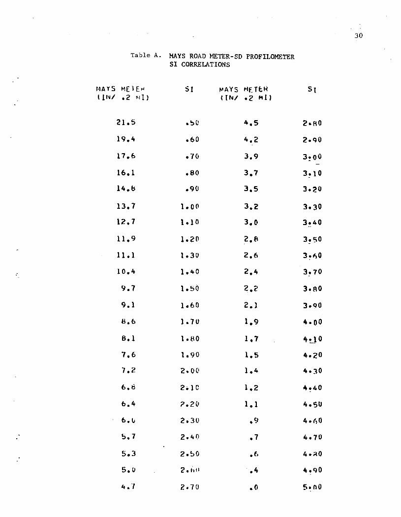
(2) The roughness measurement in terms of S1 is obtained by first measuring the length of paper (in inches) between 002-mile marks on the distance event channel, as illustrated in Fig A, and then using Table A to relate this length to S1. As noted in the figure, the 002-mile event markers were 304 inches (or 304 X 6.4 = 2108 inches of body movement per 002-mile) of strip chart movement. TableA
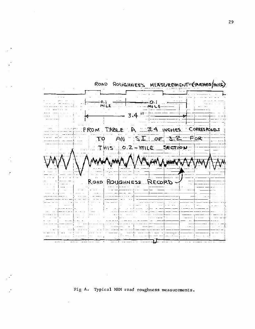
29
Ro~o _ RO·~3~K~~td_S ___ ME~~~_~!,!p~(~l*5'mHfa.) _____ --..:-1 ---, r _ 1_ ~ -- L _________ . '-
Fig A. Typical MRM road roughness measurements.
30
Table A. MAYS ROAD METER-SO PROF1LOMETER Sl CORRELATIONS
HAYS MElEtJ SI ~AYS ""ETf.H SI t INI .2 f\.1 I) ( 11''41 .2 HI)
21.5 .~o 4.5 2.AO
19.4 .bO 4.2 2.QO
17.b .7& 3.9 3!OO
16.1 .80 3.7 3!10
IIt.b .90 3.5 3.20
13.7 1.00 3.2 3.30
12.7 1.10 3.0 3.40
11.9 1.20 2.8 3.s0
11.1 1.30 2.6 3.1,0
.- 10.4 1.40 2.4 3.70
9.7 1.50 2.2 3.80
9.1 1.60 2.1 3.QO
8.b 1.70 1.9 4·00
8.1 1.eo 1.7 it!J 0
7.6 1.90 1.5 4.20
7.2 2.00 1.4 4.30
6.8 2.10 1.2 4.40
b.4 11.20 1.1 4.50
b.li 2.30 .9 4.('0
!:>.7 2.40 .1 4.70
5.3 2.!;)O .6 4.;.\0
5.0 2 • f~ II .4 4.qO
It • "' 2.70 .0 5~nO

31
provides the relationship between body movement and 81 in terms of 81 intervals of 0.1; for this example, 3.4 inches of body movement corresponds approximately to an 81 of 3.2. Because of the accuracies involved, the 81 readings need not be read beyond one decimal place and the nearest distance interval value for the appropriate 81 should be used.
MRM Tentative Operating Procedures. The operating procedures described
below should be followed closely by the MRM operators in order to insure ac
curate readings. Variations from these procedures, such as making measurements
with three people instead of two in the vehicle or with a load of cement or
samples in the trunk, can significantly affect or bias the 81 measurement.
The following tentative MRM operating procedures are recommended:
(1) Measurements should be made only under normal driving conditions. This particularly concerns weather. For instance, measurements should not be made during heavy rain, snow, extremely cold weather, or gusty wind conditions. There is also the possibility that abnormal tire pressure variations will affect vehicle body movement. Until more information can be obtained about such factors, measuring during any conditions which might directly or indirectly affect vehicle body movement should be avoided. The individual MRM operator can get a better understanding of these variations once the MRM control sections have been established, as described in the following section.
(2) For measuring during summer months, it is recommended that the Rainhart manufactured devices be installed in air-conditioned vehicles and that the air-conditioners be used during such time to help keep the MRM electronics cool.
(3) Before making a set of measurements, the MRM equipment should be visually inspected. The pens should be adjusted for proper marking and clearance before each measurement run.
(4) The manual event marker should be tested prior to each measurement run.
(5) Two operators are necessary, one for driving the vehicle and the second for operating the MRM. Their total weights should be approximately those (within, say, ±25 pounds) of the operators during MRM calibrations. The vehicle driver typically provides mileage information to the MRM operator and operates the event marker channel. The MRM operator monitors the roughness record, insuring proper operation, and makes any necessary event marks or comments on the strip chart during operations. When such notes are to be made, it is recommended that the recording device be kept on the operator's lap.

(6) When a test section has been selected, the*MRM device should be activated and an operating speed of 50 mph attained at least 0.2 mile before the beginning of the test section.
(7) Test section lengths have tentatively been established as 0.2 mile. Note that this length of measurement can be obtained by repeating runs on shorter segments and summing the paper output; that is, a O.l-mile section can be run twice and the total length resulting from both runs used as the roughness distance.
Longer sections of roadway can be sampled as desired. For instance, a
20-mile length of roadway can be represented by a continuous profile of 200
0.2-mile readings or a random sample of, say, 20 measurements taken one per
mile of roadway. Various statistics could be used to report these results,
such as the average of 200 measurements and the standard deviation or range.
Measurement Control
Accurate measurements depend on proper usage and operation of the MRM.
Proper operation of the equipment can be insured by development of a set of
control procedures in which MRM results are continually monitored.
32
These control procedure~ provide a means of detecting MRM out-of-calibration
(OC) conditions and involve the use of replicate runs or measurements Over a
known test or control section. Twenty such sections are to be established im
mediately following the initial MRM calibration procedures, providing a pool
from which more than one control section can be selected for testing for an
OC condition. The mean and range SI values from replicate control runs are then
compared against known control values determined at the time the control sec
tions were initially established.
This section describes these control procedures, which should be followed
by MRM operators in order to insure proper operation of their instruments. A
similar procedure would be necessary even if the roughness measurements were
not to be used to get SI values, to insure proper MRM operations.
Selection of MRM Control Sections. A set of twenty 0.2-mile control sec
tions should be selected convenient to the MRM base of operations. These
* Vehicle speed was set at 50 mph, as this was the speed used in developing the original 51 models for the 5DP. If a slower speed is desired, 20 mph should be used, although 51 in this case is not necessarily correct. However, we plan to develop a model for this speed as a later research activity, at which time the appropriate 51 table for this speed can be obtained.
33
sections should be selected so as to provide a representative sample of smooth
and rough sections of the area in which the MRM is to operate. The PSR varia
tions within each section should be homogeneous; that is, the roughness within
any 1/20-mi1e segment of the section should be approximately the same as in any
other 1/20-mi1e segment of the section. Obviously a smooth section with an
abrupt bump at the end of the section is not a good test section. This is a
relative measure and, in practice, will never be exactly met. However, as a
general rule, if an experienced highway technician cannot say that any particu
lar 1/20-mi1e segment of a 0.2-mi1e section rides any better than any other
segment within the section, the section can be considered homogeneous. Since
these sections are to be used for roughness control, sections where changes in
the pavement conditions are expected to be minimum should be selected, so that
the sections can be used as long as possible. Twenty was selected as the number
of sections in order to provide a large pool from which control measurements can
be made and to provide needed samples for developing the mean and range control
charts. As control sections are lost, they need not be replaced as long as four
sections remain. In a case where all but four or less sections are lost, the
MRM should be brought back to Austin for reca1ibration. The selection of the
control sections is an important part of the control procedures, since they will
be used for determining if the MRM is still in calibration.
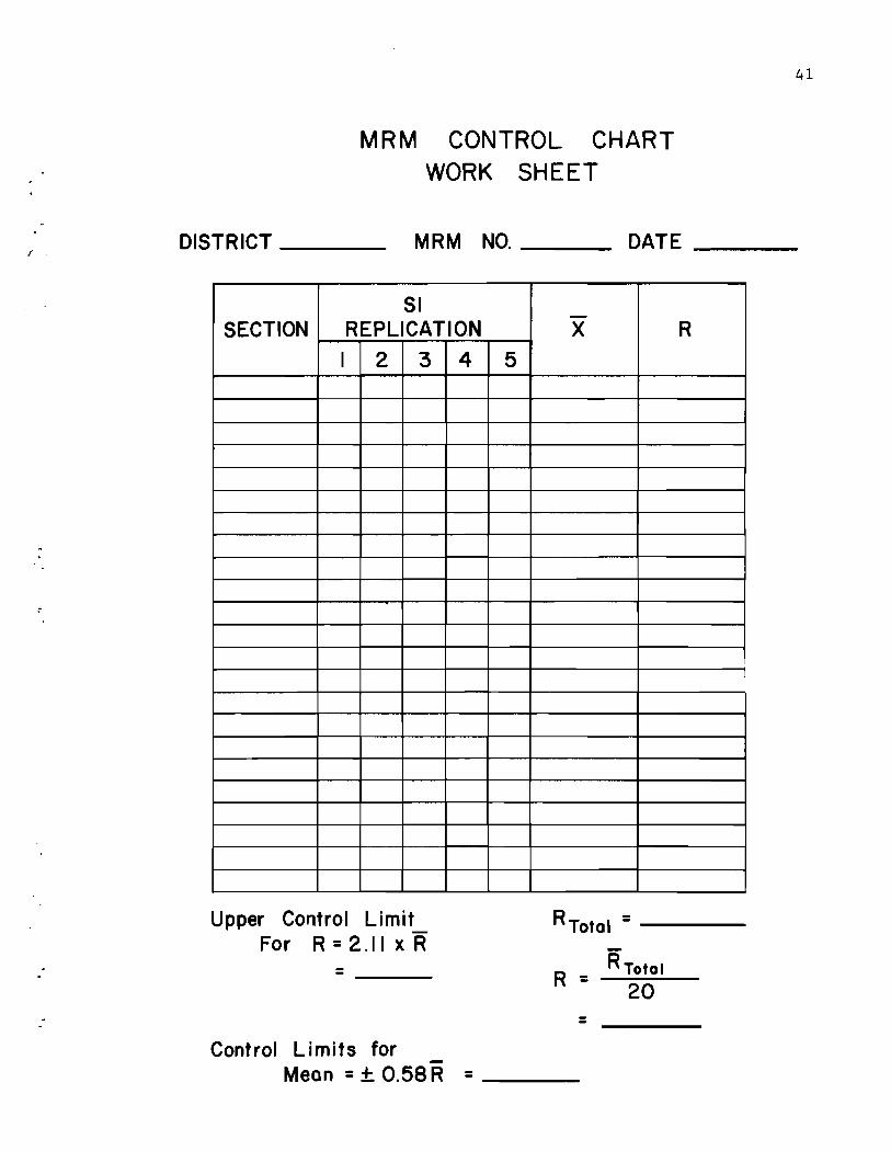
Establishing Control Charts. Two control charts are used for monitoring
MRM measurement validity, one for checking the measurement mean (or average)
from repeated SI values and the second for checking the variations from the
mean of the replicate values. The two control charts are developed with meas
urements obtained from the 20 control sections established as described above.
The range R of several MRM repeat measurements, whose mean is denoted as X,
is the greatest difference between SI values. This number is always a positive
number, or R = SI - SI min To develop the two contro 1 charts, a work sheet max
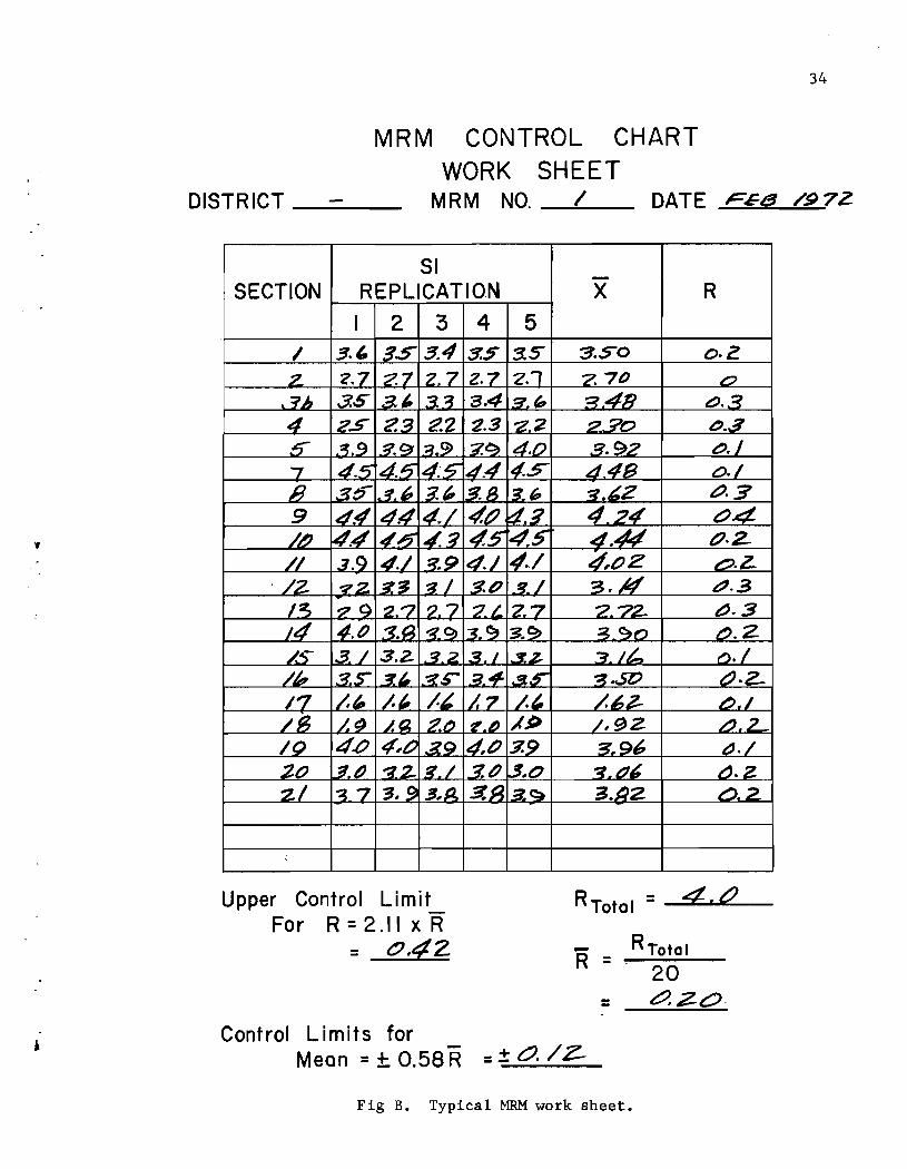
similar to Fig B is used. To compute the control limits for these charts, each
of * the 20 control sections is run five times and its SI (in terms of 0.2-mile
Since the control limits will be computed from these initial measurements, it is important to include any run-to-run or day-to-day variations to prevent these limits from being too tight. Thus, it is recommended that each section be run once and not remeasured until the other 19 sections have been similarly measured. For example, perhaps make the 20 section runs in five days so that at least one day separates replication runs.
.,
34
MRM CONTROL CHART WORK SHEET
DISTRICT ___ _ MRM NO. _..:....1 __ DATE FGI3 /97Z
SI SECTION REPLICATION
2 3 4 5
Upper Control Limit_ For R = 2.11 x R
= t:J.42
Control Limits for
x R
o.Z
17·2-.z.
RTotal = 4. (J
R = RTotal 20
= c:/. :z.o·
Mean = + 0.58 R =.± a. /Z-
Fig B. Typical MRM work sheet.
•
measurements) obtained and entered on the work sheet (Fig B). The following
values are then computed for each section:
(1) The mean X of the five test runs is computed and entered on the work sheet and the mean control chart (Fig C).
(2 )
(3)
(4 )
The range R of the five tes t runs for each section is computed and entered on the work sheet.
The mean range R is computed and entered on the work sheet.
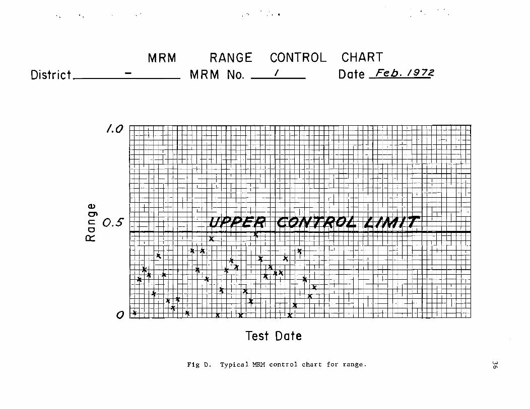
The upper and lower control limits for the mean control chart are·
computed by multiplying the mean range R by ±0.58. This value is entered on the work sheet and plotted as two straight lines on the mean control chart (Fig C).
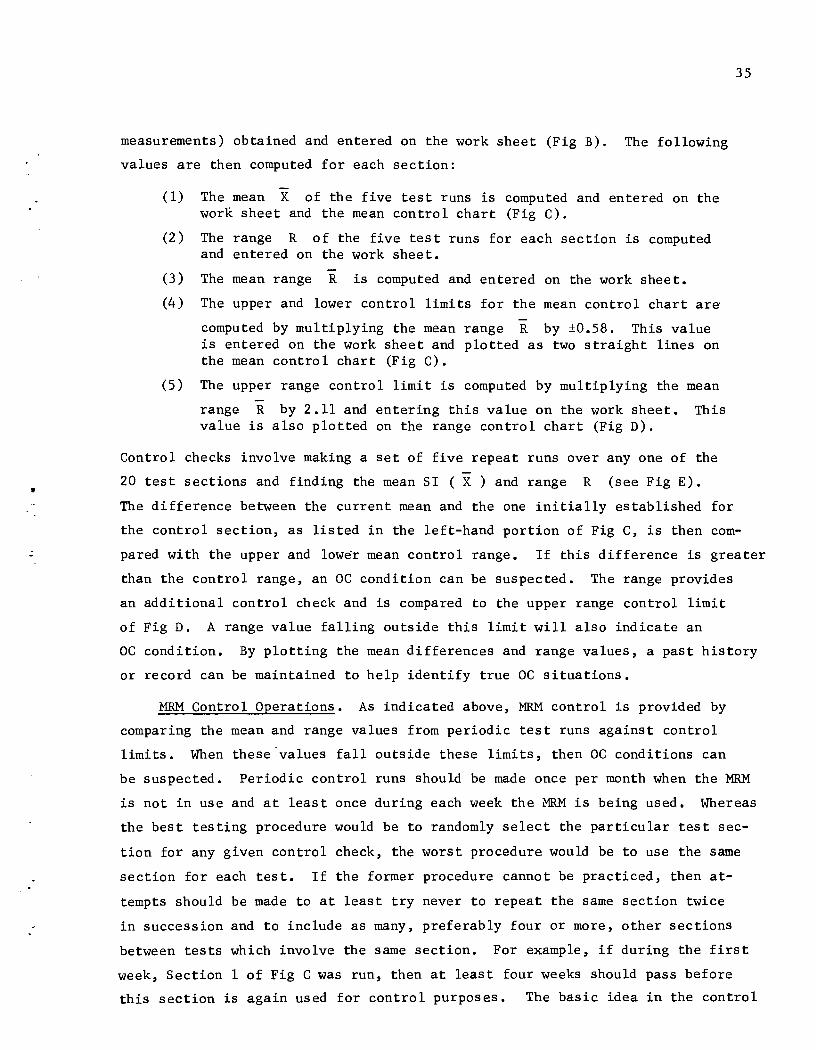
(5) The upper range control limit is computed by multiplying the mean
range R by 2.11 and entering this value on the work sheet. This value is also plotted on the range control chart (Fig D).
Control checks involve making a set of five repeat runs over anyone of the
20 test sections and finding the mean SI ( X ) and range R (see Fig E) •
The difference between the current mean and the one initially established for
35
the control section, as listed in the left-hand portion of Fig C, is then com
pared with the upper and lower mean control range. If this difference is greater
than the control range, an OC condition can be suspected. The range provides
an additional control check and is compared to the upper range control limit
of Fig D. A range value falling outside this limit will also indicate an
OC condition. By plotting the mean differences and range values, a past history
or record can be maintained to help identify true OC situations.
MRM Control Operations. As indicated above, MRM control is provided by
comparing the mean and range values from periodic test runs against control
limits. When these·va1ues fall outside these limits, then DC conditions can
be suspected. Periodic control runs should be made once per month when the MRM
is not in use and at least once during each week the MRM is being used. Whereas
the best testing procedure would be to randomly select the particular test sec
tion for any given control check, the worst procedure would be to use the same
section for each test. If the former procedure cannot be practiced, then at
tempts should be made to at least try never to repeat the same section twice
in succession and to include as many, preferably four or more, other sections
between tests which involve the same section. For example, if during the first
week, Section 1 of Fig C was run, then at least four weeks should pass before
this section is again used for control purposes. The basic idea in the control
l. . 1 •
MRM RANGE CONTROL CHART District MRM No. I Date Feb. /972
Q)
0\
1.0
c 0.5 o
0::
o
I
II IjjIII IJ ,.. I ... .. I. " I.0Il I ... If'
)
1
Test Date
Fig D. Typical MRM control chart for range.
.. "
MRM MEAN CONTROL CHART District _____ _ MRM No. __ '_ Date Feb. 1972
INITIAL MEAN
Section x 0.2 ~~-,-,-............... ...,....,.....,-,....,...
, ,
0./ +-en (J)
I-1>< 0 I
c ...... c
Ix -0./ j
I
- O. Z tt' .::t-t:i-I--i-I-L-I-~-4-J..-j.""""""....j..4...~
Test Date Fig C. Typical MRM control chart for mean.

r ,
WORK SHEET FOR
MRM CONTROL RUN
38
DISTRICT ____ _ M R M NO. _......1/:..--__
SECTION DATE ,cEI'3 1.97Z
XINITIAL (INITIAL SI AVERAGE) = _3._, ...;;;;;;~~ __ _
Run
2
3
4
5
Sum
SI
3.2...
~.4
. ~.O
3./
3./
SI = 1".3
X CURRENT = Sum SI
5
= &J .4
X INITIAL - XCURRENT = -po tlb
Fig E. Typical work sheet for MRM control run.
Enter on Ronge Control Cho'rt
Enter on Mean Control Chart

39
procedure is to determine if the MRM is giving the same measurements, within
its measurement errors. Since measurement errors can and will occur, the con
trol limits are used to identify extreme occurrences of these measurement er
rors. These errors are based on the individual MRM and the control sections
used; thus the importance of insuring proper selection of these sections and
a proper testing procedure is evident. As indicated, an DC condition can be
suspected when either the range or mean control limits are exceeded. If a
control limit is exceeded on either the mean or range (or both), the first
action, which should be immediately taken, is to carefully examine the MRM
device and the vehicle in which it is installed for the possible problem source.
If no problem source can be found, then a possible DC condition should be re
ported before further use of the instrument. If a suspected problem source can
be found it should be corrected, and then the MRM control procedures should
be performed on five of the control sections, i.e., 25 total runs. If all five
tests indicate proper operation, then no further action is necessary. If, how
ever, an DC condition again occurs on any section, it should be reported.

CONTROL FORMS
I
41
MRM CONTROL CHART WORK SHEET
DISTRICT ___ _ MRM NO. __ _ DATE ___ _
51 SECTION REPLICATION
I 2 3
Upper Control Limit_ For R = 2.11 x R
=---
Control Limits for
4 5
-X R
RTotal = ---
RTotal R=---20
=
Mean = + 0.58 R = __ _

District
INITIAL MEAN
Section
-II) ~
1>< I
o -
'. " -
MRM MEAN CONTROL CHART
MRM No. Date
1-~'----t'-t--11f--t-~-~-+---1-i-t---1--~-'-H-+' ~'--+~~f__+-i--'-Hf--t----'-+-i-+-r-_+_-'-t--i--- ---:--+--+-"-----t--+--'---~>----_+--'---~ ------,---
1--+---,---H-+--r--h-+-<--~"-t---7--,-'--t-+--,--j--+---'--+--~-+-+--H----4!--+! -+--'--------+---+-+-HJ-+-I·-'-t----'---.--I-'--+~--+ ,-t---,---,---t-,--...L....L----+ -~- .-... I-T-+--+---'-_++-'-+----i-----1I-l--i-j-.-_+-i-+-+~H-+_+__+_++_'__+_+__j___L--'---+_+_+_r__t_++-f__i_+_t_+I-+-+----;---:---t--I--!---r-.,......+-+-r--1.......L.--l-t---i-'-:'--c-I-+~~-
! ! : ---T---T-+-t---+H_+i -+-i --+' -+' --t--t-----·--'--+--1:H'----- --;-----1---~r-- -- . I I I H---t--i-H--+--t--'--+-,-,---t--r-+-i--;-; 11-+--' -I--H---'--, -+,-t--:-+-+-4--r-+--i--I---;---;,--:-'--j---:----~r----
I---c----,--t--+-+-j-'---'---'--+---.--;----'-'---'--.l--~-t-t-_+__i_.,___+___j----'_+--'-_+_+_Hc__T_+--+-_r__t_H_+-__t_ ·~H_+_+--r--i-+-+_f_-+-, --r-t--r----:-~.~- --.--;--+ 1-+--f--t--..:-.,·-+-+--:-+-+--l-~~-+--+-+-r_'_-H----'---+__'___1f_.J+__t__i_ !1-j1-+-~--t:_!_+I_+__1--+-t--H--I i I J I :-:--:----t~--+ --- . --
I i
.l "
rT-t--;-t. , ,
I I ,j J 1
-----+-+--+-:---+--r--l-,-----'--+~-+--+-H-
ttT I
I I , I 1
I , , I ' , I i I II! I
! : , 1 i . Ll J I I , I
I i
Test Date

District
Q) Cl c: o 0::
, -
MRM RANGE CONTROL CHART
MRM No. Date
i ,
,+ ++-++ u...L..L+-+-i-d--r -t t-tt-tf+ .---t---i- +-t---1,~--t--t-H~--t--+--H~--t-+-H-+--t-~-t-I~--t-+-ri~--t-+-+--t~--+-++, f---+---+-LL-<--J--t-+ I I 1 I -, T.+-';'+--~+ , +-- -+-+---t-~+-,--\---t-++-+-+-+++-H-+++-i---I-+++-H-+++-H-+-+-+-H-+++-H-+-+--I -+t+-+ ~ , r-~-t- -i---; +-+--t-+ , -->--t-+--+-t-H--t-t-1--t-t--++--f-l-+-+-++-+-+-t--f-+-+-f-+-+-f-++--l-+-t--t-t-- H LL+-t-' " +-i ' , .1 -t+ I I I I ,
H--t-'+-:l-t--t--+--t--+-+-hH--+-' -+-+--+'-:~ ~~+T+--~ J
I ! ! 'I I
Test Date

.-
WORK SHEET FOR
MRM CONTROL RUN
44
DISTRICT ____ _ MRM NO. ____ _
DATE _____ _ SECTION ___ _
XINITIAL (INITIAL SI AVERAGE) = _____ _
Run 51
2
3
4
5
Sum SI = ==
X CURRENT = Sum SI
5 =---
RANGE = SIMAX-SIMIN = __ _
XINITIAL - XCURRENT = ---
Enter on Range Conttol Chort
Enter on Mean Control Chart

APPENDIX 2
DESCRIPTION OF MAYS RIDE METER
The Following are
Excerpts From
MAYS RIDE METER BOOKLET (Ref 9)
and are Pertinent to This Investigation
46

The incomparable 47
MAYS RIDE METER for pavement surveillance
Purpose-The MAYS RlDE METER is used to most conveniently and economically evaluate or compare pavement surfaces; a practical, and significant record is immediately available interpretation in field or office
Uses-MAlNTENANCE • He:p decide where besl to spend available funds • Evaluate before-and-aiter overlaymg Or surface treatment • Ear:y warning can signal preventive maintenance before
pavemer1t or base failure. • Assisl in dispatching repair crews
CONSTRUCTION • Evaluate base coarse smoothness 11ft by hit • Pavement acceptability.
INVENTORY MANAGEMENT • Surveillance over months or years
RESEARCH
"":#'.' .,
...
The MAYS METER IS an mexpenslve instrument that continuously logs the pavement surface by recording magnitude, direction and summallon of rear axle 10 body excursions of its parent automobile together with synchronized distance incre· ments and landmarks ThIS portable instrument, tethered by an electrIC cord, 15 placed In the lap or on Iront seat and is operated al tra:[ic
The record IS a SIX inch w;de "2" {old chari (see center spread) uniquely fed 01 a variab:e rale sum roughness Ivan K Mays deserves lull credit [or thIS breakthrough On this chart is supeli:nposed three synchronized traces which display
• SUMMATION of roughness over any desired distance; • NATURE of the roughness, • LOCATION oj pavement defects. • MILEAGE licked oli by 1I20th mile increments; • LANDMARKS and • FIELD NOTES simultaneously jotted on the chart with oc"
currence of the happening.
Patent No. 3525257
S9jl 1-72
.....
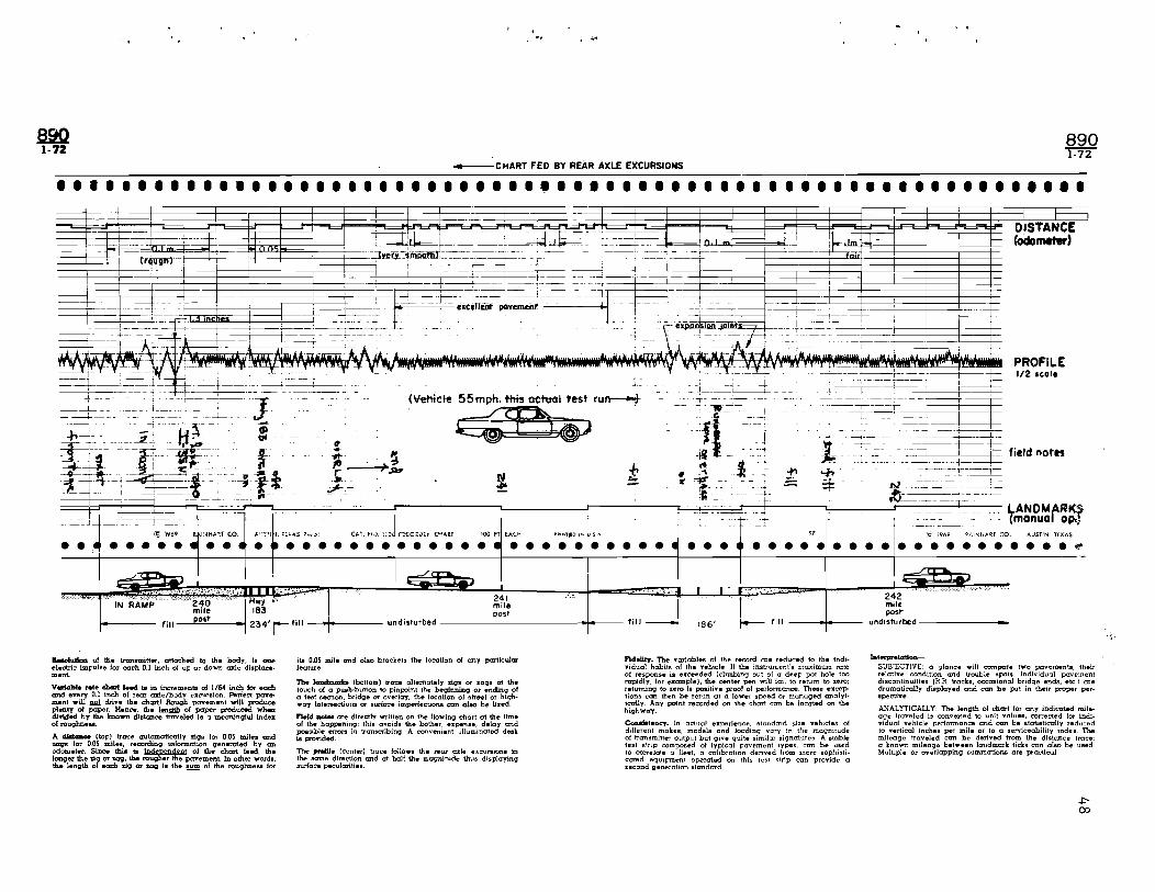
_CHART FED BY·REAR AXLE EXCURSIONS
890 1-72
•• I I I I I I I I I • I I I I I I • I • II I I I I I I I, I I. I I I • I I I I I I I I I I I I • I I I I I I' I I ••• I
~-=r::== _
. .......-I I
IN RAMP' fiU_··_'···_·:",:,:",:t";·_·"·_O:,_'._"' .. ",,. ;:' ~"" _~~.,.. ____ undisturbed _____ ~_:_;~I_~ ______ -.. ____ fill ~
186' fi II --~-+----
IIMohd:la:l of the transmitter, attacbed 10 the body. 18 ODe electric impulse for each 0.1 inch or up or down axle displace· menL
Yadahle rote chart feed ts in increments 01 1/64 inch tor each and every 0.1 inch of rear axle/body ex~ion Perfect paT. menl will ml1 drive the chart! Rough pavement will produce plenty 01 paper. Hence. the ~ of paper produced when d.1't'\d.ed by the known dis~ce traveled i8 a meaningful index 01 roughnell8.
A dltdcmce (top) ~race automcrtically ziga lor O.OS miles and ZayII lor 0 OS miles, recording inlormation generated by aD
l!o:;t:~ ~~O: :: ~ !t:=:en~e:e"nt.t~tht;r~o::: the length of each dg or zag la the!!!.!!! of the mughnell8 lor
it. 0.05 mile and olso brockets the location of any particular feature
The Icmdmmb (botlom) b'ace altemately zigs or zag8 at the touch of a push·buHon to pinp::lint the beqlnning or ending of a test sechon, brIdge C1r overlay; the location 01 street or highway iDler~ctions or surface imperfections I;.1m aJ.eo be !ixed
raeld aot .. are directly written on the !lowing chon crt the lime 01 the happening; this avoids the bolher, upense, delay and possible errors in transcribing A convement illuminated desk is provided.
The praIiIe (center) trace follows the rear axle elfCUn!llOnS in the same direction and at hall the mavnilude thus displaying IJUTlace pecularities.
ndelity. The variables of the record me reduced to the indi· vidual habits 01 'he Yehicle 11 the instrument's maximum rate of response is exceeded (chmblng out 01 a deep pot hole too rapidly. lor ezample), the center pen will lail to return to zero; relumino- to zero I, positiYe proof oJ perlormance. These exceptions can then be rerun at a lower speed or manco-ed analyt. lcally Any potnt recorded on the chari can be located on the highwCll'.
Conallteacy. In actual experience, standard 5ize vehicles of dIfferent makes, models and loading vary in the magnitude of transmiHer output but give quite similar signatures A stable test strip composed of typical pavement types, can be uSEd to correlate a lIeet, a calibration derived Irom more sophisti· cated equIpment operated on this test strip can provide a second generation standard
242 mile post"
undisturbed -------_
JalftPhtcrtiOD-
DISTANCE (odometer)
PROFILE 1/2 Ical.
field notes
SUBJECTIVE' 0 glance will compare Iwo pavements, their relative condition and trouble spoLs. Individual pavem~nt discontinuities (R R. !racks. QCCc:mional bridge ends, etc.1 are dramatically displayed and can be put in their proper per-8pective.
ANALYTICAllY: The length 01 chart for any indicated mile· age traveled is convened to unit values, c:orrected lor individual vehicle performance and can be statistically reduced to Yertical Inches per mile or 10 a serviceability indelf 1be mileage traveled can be derived nom the distance trace; a known mileage belween landmark ticks can also be uaed Multiple or overlapping summations are practical
. ~.

Electromc circuita-The top and bottom pens are solenoid activated: • the distance pen is controlled by a special odometer containing a microswitch which is automatically cam actuated to alternately make for 005 miles and break for 0.05 miles; and • the landmarks pen is controlled manually by a push-on push-oil switch.
The transmitter, permanently installed in the trunk, has a 4 track mylar film program mounted in its direct drive, axle attached shuttle; this program is read by 4 tiny (\ 1\6 in. dia.) photocells whose output is relined at the recorder by the first r c. (integrated circuit chip) and controls a 4 track. two stage amplifier transistor-switch card; hence. the high response oscillating stepper motor drives the profile (centerl pen employing a rack-and-pinion.
These relined impUlses from the lirst LC. are also fed into a second LC. which unscrambles and a third I.C. (a Ilip-flop) which reprograms them to control a second 4 channel 2 stage transistor-switch card; thus the chart drive stepper motor rotates in a fixed direction one step for each and every transrrlitter generated impulse. The two identical 4 phase stepper motors are RIC excited. All components (photocells. solenoids, exciter lamp. stepper motors and chips) are 12V DC and are compatible with automobile 12 volt, negative ground electric systems.
CAT. NO. 890 MAYS RIDE METER-Complete with solid state recorder; photoelectric transmitter, modified odometer, required connections; three pens; 1006 Recorder Chart, Pkg. 300 ft; and Mays Ride Meter Booklet. Approx. Ship. WI. 40 lb.
CAT. NO. 1006 RECORDER CHART, PKG/300 n.-Three 100 II lengths for use with 890 Mays Ride Meter. Approx. Ship. WI. 2 lb.
49
Specifications-The recorder provides a record of road surface roughn'?ss from the relative motion between body and rear axle housing of a tull size. solid rear axle automobile. The recorder and associated systems employ electrically transmitted data utilizing current solid slale design in all circuits. The transmitter detects both direction and magnilude of relative vertical motion between the automobile body and rear axle housing with 0.1 inch resolution. Its range and reo sponse allows operaiion of the Instrumented vehicle over normal surfaced roads at speeds in excess of 50 miles per hour under normal safe driving conditions. The transmitter out put commands the pavement profile (center) pen to duplicate rear axle excursions at hall scale and to also advance the chart paper 1/64 inch lor each 0.1 inch increment 01 excursion both up or down. The distance (top) trace automatically records 0.05 mile increments; this pen is controlled trom a special odometer The landmarks (boltom) trace (providing pinpointing of any associated event) is push-button controlled; a desk is provided (allowing convenience when writing Held notes simultaneously with the happening) The 6 in~h cast aluminum recorder employs sprocket driven (lor positive drive) Z~rold chart pack (for quick and convenient acceS.3 to the recorded data). Flip-up loading is provided (to eliminate chart threading). A desk light is turnished (lor convenience in alter-dark operation). The recorder employs easy access for service and maintenance of all electric and mechanical components Plugin printed circuit boards are used (to allow in-field replacementJ~ Electric cabling allows freedom 01 recorder location and operation in any nem horizo'1:al position in the front seat of the automobile; when unplugCled. the recorder can be removed from the vehicle The entire system operates from a nominal (no modifications necessary) 12 V DC negative ground automobile power system
Additional information including vehicle recommendations, operating instructions, interpreting guide and installation are contained in your Iree copy 01 the Rainhart Cat No. 890 MAYS RIDE METER BOOKLET.
~COPY~lght by RAIN HART Co 600-8 Wlll!ams St., POBox 4533, AustIn, Texas 78751-Tel.5121452-8848

History. Pavement roughness measuring devices using the
car's body as a reference platform and a wheel or axle as a
sensing device can be traced back to the early 30's--there is
nothing new here. The hang-up has been inventing a practical
format for the data. Mr. Mays' variable rate of chart feed
allowing continuous summation of roughness, is the breakthrough.
His is the most practical system of data presentation which
has been advanced.
This is a second generation instrument replacing the
original Mays Road Meter (described in several highway pub
lications). The changes improve:
o convenience (a lap or front seat instrument replacing the original rigid trunk location);
o' accurac~ (solid drive digital transmitter replacing cord drive with spring take-up);
o ~ of interpretation of the record (three side-by-side pens mounted on a common track replace swing pens which were staggered along the record), and
o distance is recorded by 1/20th mile increments instead of l/lOth.
The unique presentation of data has been carried forward!
Vehicle. The Mays Ride Meter faithfully records the ride
50
of the rear of an automobile: this makes the vehicle the critical
element in the apparatus (as well as the expensive portion of
the package).
The car body is the reference platform for all measurements
and hence the title: Ride Meter. To use an absurd but appropriate
illustration: if the rear axle were unsprung (solid blocking, no
springs or shock absorbers like an ox cart), the Ride Meter
transmitter would generate no signal and the recorder would call
all pavement perfect! (For ox carts, that is!) The Detroit
"boulevard-ride" is highly desirable! But even this can be overdone.
Dimensions: A portable instrument; width 11 inches, length 18 inches, height 8 inches, weight 17 lb. Operates on l2V DC negative ground automobile systems.
An ideal vehicle would have:
o a full size body
o front engine
o solid rear axle
o coil springs (leaf springs tend to depart from Hook's Law because of internal friction of the scrubbing leafs)
51
o drag links (to keep the axle from wandering fore and aft)
o rear sway bar (to prevent the axle from wandering laterally)
o firm_shnck abRorbers (the suspension must be hard enough to not bottom out readily but soft enough to generate adequate transmitter action) VERY IMPORTANT
a round tires (preferably ground since cyclic out-ofroundness will appear as surface roughness)
o dynamically balanced tires (ditto)
o a sufficiently accurate original equipment odometer and speedometer. (Tire circumference is the most frequent culprit. Automobile dealers can furnish a variety of transmission/speedometer take-off gears--one tooth difference is about 5%)
o and air conditioning. (This is highly desirable in hot climates quite as much for the reliability of the electronic components as fo"r the comfort of the crew. All solid state circuitry operates more reliably in a cool, dry environmentj stepper motors and large resistors dissipate heat more readily).
Tire pressure, temperature (particularly of the shock ab
sorbers), weight of load and amount of gas in the tank, also
affect the ride.
The above is offered as a guideline for optimum instrument
utilization. Actual experience in comparing the variations
among well sprung and damped vehicles shows that the differences
are primarily in amplitudej the signature is not significantly
affected.
Driver factor. In addition to the unique mechanical
characteristics of the vehicle, the record also reflects
driver behavior. Only by traveling at a constant velocity
guided smoothly along the wheelpaths can a true picture emerge.
The rear of the car squats when accelerating and lifts when
braking thus generating pitching; the vehicle rolls when
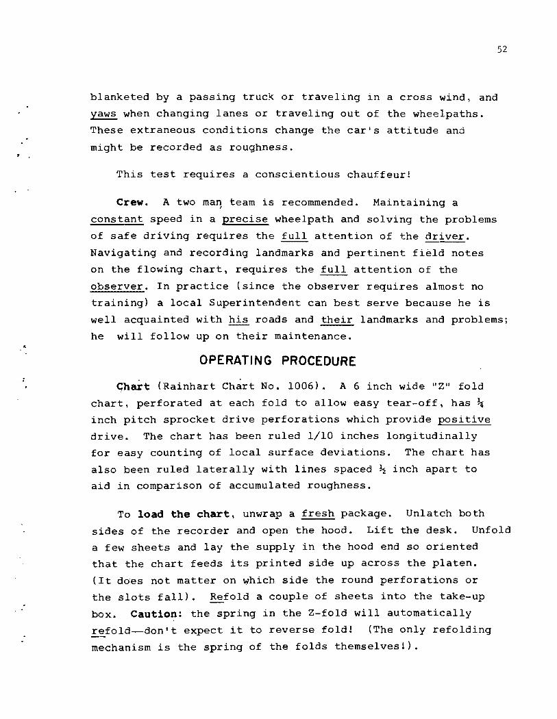
, .
blanketed by a passing truck or traveling in a cross wind, and
yaws when changing lanes or traveling out of the wheelpaths.
These extraneous conditions change the car's attitude and
might be recorded as roughness.
This test requires a conscientious chauffeur!
Crew. A two ma~ team is recommended. Maintaining a
constant speed in a precise wheelpath and solving the problems
of safe driving requires the full attention of the driver.
Navigating and recording landmarks and pertinent field notes
52
on the flowing chart, requires the full attention of the
observer. In practice (since the observer requires almost no
training) a local Superintendent can best serve because he is
well acquainted with his roads and their landmarks and problems;
he will follow up on their maintenance.
OPERATING PROCEDURE
C;hart (Rainhart Chart No. 1006). A 6 inch wide liZ" fold
chart, perforated at each fold to allow easy tear-off, has ~
inch pitch sprocket drive perforations which provide positive
drive. The chart has been ruled 1/10 inches longitudinally
for easy counting of local surface deviations. The chart has
also been ruled laterally with lines spaced ~ inch apart to
aid in comparison of accumulated roughness.
To load the chart, unwrap a fresh package. Unlatch both
sides of the recorder and open the hood. Lift the desk. Unfold
a few sheets and lay the supply in the hood end so oriented
that the chart feeds its printed side up across the platen.
(It does not matter on which side the round perforations or
the slots fall). Refold a couple of sheets into the take-up
box. Caution: the spring in the Z-fold will automatically
£~fold--don't expect it to reverse fold! (The only refolding
mechanism is the spring of the folds themselves!).
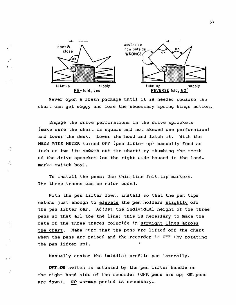
, .
.. open a
close
toke-up supply RE- fold, yes
was inside now outside
WRONG!
toke-up supply REVERSE fold, NO!
53
Never open a fresh package until it is needed because the
chart can get soggy and lose the necessary spring hinge action.
Engage the drive perforations in the drive sprockets
(make sure the chart is square and not skewed one perforation)
and lower the desk. Lower the hood and latch it. With the
MAYS RIDE METER turned OFF (pen lifter up) manually feed an
inch or two (to sm~Qth out the chart) by thumbing the teeth
of the drive sprocket (on the right side housed in the land
marks switch box).
To install the pens: Use thin-line felt-tip markers.
The three traces can be color coded.
With the pen lifter down, install so that the pen tips
extend just enough to elevate the pen holders slightly off
the pen lifter bar. Adjust the individual height of the three
pens so that all toe the line; this is necessary to make the
data of the three traces coincide in straight lines across
the chart. Make sure that the pens are lifted off the chart
when the pens are raised and the recorder is OFF (by rotating
the pen lifter up).
Manually center the (middle) profile pen laterally.
OFF-ON switch is actuated by the pen lifter handle on
the right hand side of the recorder (OFF, pens are up; ON,pens
are down). NO warmup period is necessary.

Velocity. ~he performance of any vehicle is sensitive to
velocity. On fair-to-good pavement, 50 mph. is recommended.
If recording long undulations of otherwise smooth pavement,
54
much higher velocities, perhaps up to 70 mph., will be required.
On the other hand, when running city streets or poor pavement,
much slower velocities (perhaps 25 mph.) is not unreasonable
and 10 to 15 mph. may be quite fast enough in extreme roughness
or railroad track crossings that are in bad need of repair.
The velocity must match the task in hand!
Avoid velocities associated with the vehicle's natural
resonance points.
Test run. With the Mays meter loaded and checked out
and the vehicle stabilized at the desired velocity and
direction, lower the pens shortly before the road test is
to begin. Coincidentally with starting the run, zero the
odometer and press th~ landmarks button. Record landmarks,
observations and pertinent data such as:
run number; date; time; location or highway number;
direction of travel; lane traveled; length of test run;
weather; etc.
Make sure that enough data is gathered and recorded-- these
rapidly accumulating records are impossible to sort out from
memory.
When finished, mark the end of the run, raise the pens
and manually advance the paper until the pens are across the
next (perforated) fold--a convenient tear-off. Decide if the
record is usable--if not, modify the procedure and rerun.
Tracking rate. The response of the stepper motors is
faster than 10 milliseconds (1/100 second); this will track
roads in poor condition and railroad corssings at reasonable
velocities. The recorder will either track with complete
fidelity or will fail to return to its arbitrary zero telling

f'
55
the operator that axle excursion velocity exceeds the instrument's
ability to read thus saying: "Rerun slower, please!" Turning
the recorder OFF (by lifting the pens with the pen lifter lever)
will unlock the steppe~ motors electrically and allow manual
profile pen rezeroing or chart advance.
Comparing traces. There is no physical reason for £ot
changing color code and superimposing a rerun on the same
(refolded) chart. In practice, however, it is more practical
to make runs on independent strips and compare them side by
side thus allowing the strips to be moved longitudinally to
establish the most convenient match for any area under scrutinization.
RECORD a INTERPRETATION
-tt-.05 -1 --un rl----~L__
~"ko., -' (smooth) (rOugh)!
Mileage Trace
(1) Distance (top trace),is controlled
by a special odometer, zigs for 0.05 and
zags for 0.05 miles; one complete cycle
= 0.10 miles. The distance the vehicle
~raveled is recorded independently of
chart feed.
(2) Profile (center pen) records the axle/body excursions at
~ of the actual vertical distance traveled. The pen moves by
steps of 1/20 inch at the command of each impulse from the
transmitter (1/10 inch). This pen is rack-and-pinion driven by
a stepper motor (located on the top of the instrument hood); the
motor reverses with each change in axle direction. Inconsequential
axle movement of less than 0.1 inches is filtered out at the
transmitter and is not recorded.
The nature of the pavement roughness is indicated by the
profile (center) trace. A pothole, dip or swell will be re
corded as a wide undulation
spread over lots of chart length; short waves of consistant
roughness will appear as uniform

A
narrow amplitude, and very long waves will appear when the
car's velocity is high enough to respond.
(3) Landmarks are indicated near the bottom of the chart as
zigs and zags responding to the operator's push button com
mands to pinpoint the location of the happening (event mark).
A convenient desk assists in keeping a play-by-play score
card on the flowing chart eliminating the bother, expense or
danger of errors in transcribing field notes. A pilot/desk
lamp in the handle allows arter-dark operation.
Roughness summation. ~he chart, driven by a second (but
identical) stepper motor (located on the left side of the
recorder), is moved 1/64 inch for each l/lOth inch or 1 inch
56
for each 6.4 inches of total axle vertical travel (64 impulses).
Each impulse (representing 0.1 inch axle movement) from the
transmitter drives the profile pen up or down one step; it also
drives the chart one stoep! This unigue feature allows roughness
to be summed continuously.
The Mays Ride Meter drives the chart 5 inches for every
32 inches of (total) vehicle axle vertical travel: the length
of chart produced in a mile (indicated by the distance or
landmarks trace) multiplied by 6.4 equals the total amount
of axle excursions in inches per mile as referenced by the
axle to body movement.
The less chart produced in a standard distance traveled,
the smoother the pavement. And vice versa.
Since the amount of axle movement generated by the highway
will vary with the vehicle and its condition, a multiplier must
be determined if the unit quantity of chart is to be correlated
wi th the vertical inches of pavement roughness as determined by
other measuring systems. This suggests:
A standard local test course. A conveniently located mile
of stable (and not too heavily traveled pavement) should be

t .
•
. , ..
57
used as a local second generation standard. It would be ideal
if several qualities of pavement were represented in this stretch.
This lane can be occasionally calibrated with more sophisticated
pavement evaluation equipment if it needs to be correlated; or
a vehicle factor can be derived to take into account the car's
individual habits .
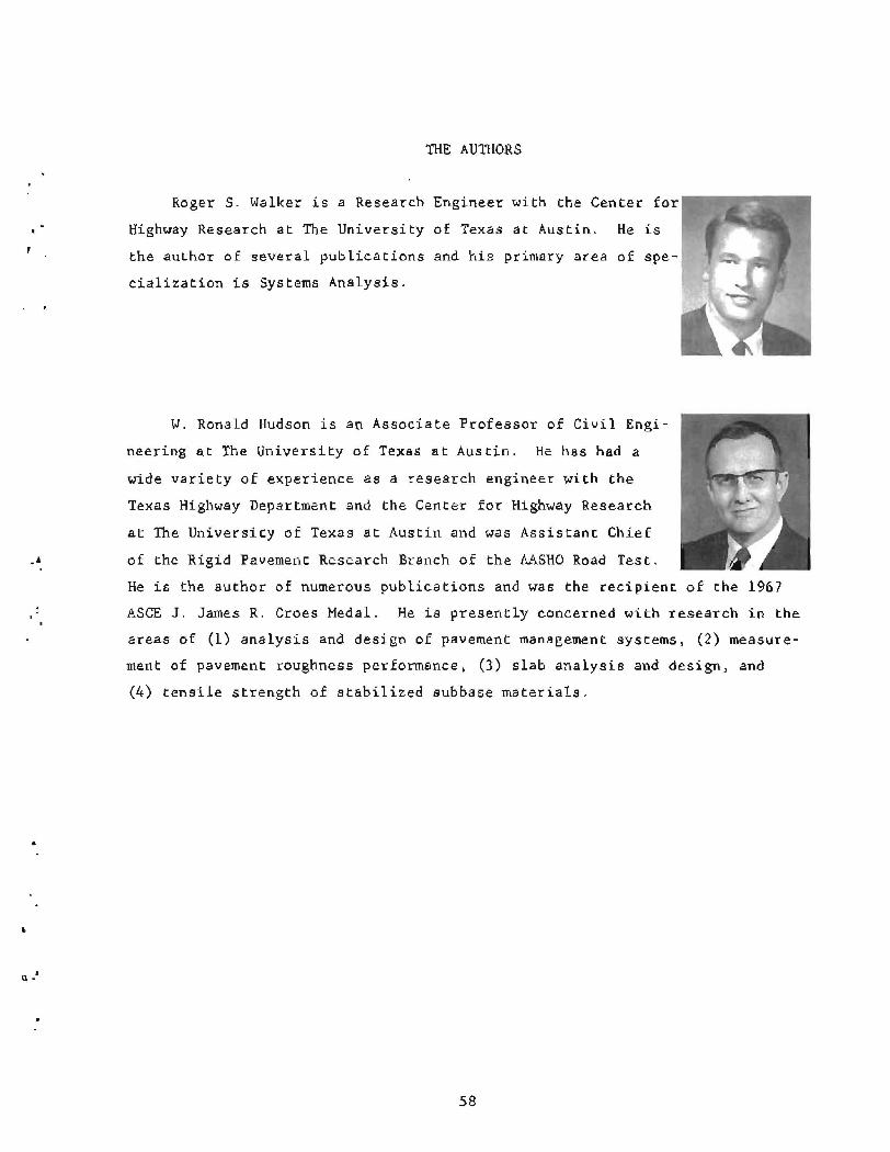
. '
I \l, •
THE AUTHORS
Roger S. Walker is a Research Engineer with the Center for
Highway Research at The University of Texas at Austin. He is
the author of several publications and his primary area of spe
cialization is Systems Analysis.
W. Ronald Hudson is an Associate Professor of Civil Engi
neering at The University of Texas at Austin. He has had a
wide variety of experience as a research engineer with the
Texas Highway Department and the Center for Highway Research
at The University of Texas at Austin and was Assistant Chief
of the Rigid Pavement Research Branch of the AASHO Road Test .
He is the author of numerous publications and was the recipient of the 1967
ASCE J. James R. Croes Medal. He is presently concerned with research in the
areas of (1) analysis and design of pavement management systems, (2) measure
ment of pavement roughness per £0 ITII8nCe • (3) slab analysis and design, and
(4) tensile strength of stabilized subbase materials,
58


