
A Novel Image Database Analysis System for Maintenance of Transportation Facility – Phase I
The University of Toledo – University Transportation Center
Project Number: UTUTC-IU-5
Final Report
Eddie Y. Chou Principal Investigator
Ezzatollah Salari Co-Investigator
June 2010

DISCLAIMER
The contents of this report reflect the views of the authors, who are responsible
for the facts and the accuracy of the information presented herein. This document
is disseminated under the sponsorship of the Department of Transportation
University Transportation Centers Program, in the interest of information
exchange. The U.S. Government assumes no liability for the contents or use
thereof.

A Novel Image Database Analysis System for Maintenance of Transportation Facility – Phase I
Executive Summary
Transportation is critical to the global economy and plays a particularly vital role in this region’s
economic growth. Transportation infrastructures such as highways, streets, and bridges represent
one of the largest public investments of many governments. Maintaining and managing the vast
and aging transportation infrastructures with limited resources is a most challenging task for
nearly all transportation agencies. Monitoring and evaluating the physical condition of the
transportation infrastructure and scheduling for timely repair are essential for effective
infrastructure management. However, human inspection can be time consuming and prone to
inconsistent results due to differences in judgments. Digital imaging technology has
been proposed as a viable alternative to human inspection and provides automated
inspection, monitoring, and pattern recognition, as the cost of imaging technologies has
become more affordable. The objective of this research was to assist transportation agencies
efficiently record, monitor and evaluate the conditions of transportation infrastructure
assets so as to more effectively managing the needs for maintenance or rehabilitation with
minimum total costs and least interruptions of services. The researchers reviewed relevant
literatures and designed the framework of a prototype imaging system to systematically and
automatically extract features from digital images of pavement surfaces. The focus was on
processing and transforming the roadway images for analysis, and extracting visible cracking
data including crack length, width, and patterns from the processed roadway images. A new
crack connectivity algorithm to rebuild the crack pattern after noise reduction was developed
and implemented. This study was jointly funded by UT-UTC and MIOH-UTC. Phase II of this
project, which continues the development of the prototype and focuses on improved
quantification of cracking in terms of its length and width, and uses wavelet transformations to
extract and identify different crack patterns in order to match the imaging processing results
with human ratings, was subsequently funded by both sponsors.

1. Introduction
Transportation infrastructures such as highways, streets, and bridges represent one of the largest
public investments of many governments. Maintaining and managing the vast and aging
transportation infrastructures with limited resources is a most challenging task for nearly all
transportation agencies. Monitoring and evaluating the physical condition of the transportation
infrastructure and scheduling for timely repair are essential for effective infrastructure
management. However, human inspection can be time consuming and prone to inconsistent
results due to differences in judgments. The demands for automated inspection, monitoring, and
pattern recognition for transportation applications are ever increasing, partly driven by the costs
of imaging technologies which are becoming more affordable. There are two major steps in the
development of an automated pavement evaluation system, namely, image acquisition and
software development of image processing algorithms for data analysis and interpretation. This
study focuses on the development of image processing techniques for pavement surface anomaly
detection and characterization. This includes extraction of pavement abnormalities in a digital
image from the background and obtaining a binary image leading to the characterization and
quantification of the pavement cracks.
A typical inspection process such as pavement distress inspection can be divided into three
stages: preprocessing, segmentation, classification and measurements. Preprocessing is used to
improve the quality of the input image in order to facilitate the analysis and interpretation at
subsequent stages. One of the important tasks in preprocessing is filtering for noise removal,
deblurring the image, or highlighting specific features, e.g., cracks on the pavement to meet the

demand of the application concerned. Image segmentation is the process of dividing an image
into meaningful regions, namely, objects of interest and background. The main parameters of
interest for pavement inspection are crack pattern classification and measurement of various
parameters from crack features.
This report explores the existing digital imaging technologies to automate the pavement
condition assessment process. The main parameters of interest are pattern classification and
measurement of various parameters from crack features. Section 2 reviews the previous works
on processing pavement images. Section 3 presents the methodology developed as a result of
this study. Section 4 shows the simulation results and the progress in achieving the goals set for
this project, followed by the conclusions in Section 5.
2. Background
The wavelet transform methods have been employed by some researchers as a crack detection
tool. The advantage of the wavelet transform is its multi-resolution property, which allows
efficient identification of local features of the signal [1]. The wavelet transform has been
successfully applied for crack localization in beam structures [2], [3]. The Lipschitz ecponent is
used to estimate the size of the crack [4]. Douka proposed a method for estimating both the
location and size of the crack by defining an intensity factor which relates to the size of the crack
to the coefficients of the wavelet transform [5]. Li Qingquan [6] proposed a robust and high-
efficiency model for segmentation and distress statistic of massive pavement images which based
on multi-scale space. S. K. Sinha [7] proposed a method for detection of crack falls within the

scope of the Bayesian framework. Leontios,Evanthia and Athanasios proposed algorithm for
crack detection called kurtosis crack detector (KCD) [8]. Above, people have done some
research about crack detection, and now we will concentrate on crack connection problem.
H.D.Cheng [9] proposed a method which can check connectivity of cracks using the fuzzy set
theory. The objective is to eliminate pixels lacking in connectivity. The isolated darker pixels,
which are considered noise, are eliminated. Although many noise pixels are removed the method
still cannot connect break points of cracks in their experiment results. In other words, cracks are
not very clear after checking connectivity. There are a few papers mentioned about checking and
connecting break points of cracks. The proposed algorithm in this paper provides a new method
to easily count the number of cracks. The Strategic Highway Research Program uses 4-
connected algorithm to connect cracks and remove spurs of cracks. First the method needs to
convolve the image. If the diagonal pixels are black, the near up or bottom pixel is also given
black. Then it removes spurs of the image. If one pixel has less than two black pixels in its four
neighbors it will be removed as a spur pixel. The test results show effect in connecting the break
points. However, it cannot reflect accurate direction of cracks because of removing crack pixels.
Y. Huang and B. Xu [10] proposed the crack cluster connection method. First, it finds verified
seeds of crack, and then connects individual seeds into seed clusters. Starting from one seed, a
crack cluster grows by accepting adjacent seeds one at a time until no close seeds can be taken.
It can be used to draw a path in the corresponding pavement image but it is hardly able to
calculate the width of cracks.

3. Methodology
The image processing technique developed in this study operates on existing digital images of
pavement surface. First, digital image preprocessing is performed to convert the original image
to binary image, enhance the images, and remove any noises. After typical noise reduction
operations, some cracks would become „broken‟, that is discontinuous due to the noise
reduction process. Therefore, a crack connectivity algorithm was developed to reconnect the
cracks. The
algorithm first finds the initial pixel of a crack and decides the direction of the crack, for
example, whether or not the crack is transverse or longitudinal. The algorithm then searches in
each direction for break points of cracks. After finding a break point, the algorithm locates the
nearest crack pixel in a particular searching area to fill the gap. When the pixels between it and
the break point are filled, the nearest crack pixel will be the next initial pixel. The algorithm
continues to search the break points until the end of the crack is located. The entire processing
methodology is shown in Figure 1.
3.1 Image Enhancement
The aim of preprocessing in pavement image inspection is to suppress the unwanted information
from the image data and enhance the desired image features important for further processing.
Preprocessing is an important step in the sense that with an effective pre-processing much of the
subsequent analysis will be simplified.
Due to non-uniform lighting or weather conditions, the contrast between distresses and
background is often very low. In addition, the image is often corrupted with noise and undesired

features. Therefore, an image enhancement method capable of removing non-uniform
background illumination effects and noises is required.
Input pavement image
Obtain enhanced image by nonlinear
filtering
Obtain binary image by
thresholding
Fill gaps by dilation and erosion
Eliminate isolated noise
Connect break points
Figure 1 Processing Steps
A promising technique would be to use a nonlinear filter which takes the mean and variance of
local gray values into account. Other techniques, such as median filtering can be used to reduce
the noise while preserving much of the details in the image. To remove the non-uniform
background intensity effect, we used the following nonlinear filter, as show in (1),
f*= Z(i,j)* [forg(i,j)-fblur(i,j)]+m (1)

where f*
, forg(i,j),and fblur(i,j) are respectively the filtered, original and blurred images of the
pavement, m is the mean value of the original image, and Z(i,j) is a local gain factor sensitive to
local variations which is 1 for here. The blurred image is obtained by convoluting a low-pass
Gaussian spatial filter [8] with the original image. Here, we chose Gaussian low-pass spatial
filter because it avoids a bright ringing effect.
3.2 Thresholding
Thresholding is a widely used technique for image segmentation and feature extraction. For a
given image, most of these techniques involve creating a histogram of the gray level values to be
used to find the peaks that exist in the image. A threshold is then chosen according to the valley
between these peaks or modes (usually two prominent peaks are assumed). Adaptive
thresholding applies a different threshold to different regions of the image and results in better
segmentation. Pavement cracks usually involve abrupt changes in gray level of two adjacent
regions of variant gray levels. With an appropriate threshold that is extracted from the block and
lies somewhere between the means of the two regions, the block can be binarized.
Here, we use a segmentation method based on fractal theory. A fractal is generally a rough or
fragmented geometric shape that can be split into parts, each of which is (at least approximately)
a reduced-size copy of the whole, a property called self-similarity. The term was coined by
Benoît Mandelbrot in 1975 and was derived from the Latin fractus meaning "broken" or
"fractured." a mathematical fractal based on an equation that undergoes iteration, a form of

feedback based on recursion. Following Ref. [11], first, we introduce the concept upper surface
and lower surface . Initially, given the gray level function
. For . The upper surface and lower surface are defined as follows:
(2)
(3)
The image points (m,n) with distance less than one from (i,j) were taken to be the four immediate
neighbors of (i,j). The covering blanket is defined by its upper surface and its lower surface. A
point will be included in the blanket for . The volume of the
blanket is computed from u and b by
As the surface area measured with radius we take the volume divided by
(4)
(5)
The area of a fractal surface behaves according to the expression:
(6)
After taking logarithm of expression (6), we get the equation:
(7)
According to the expression (7), the slope D and the values of k can be calculated by least-
square fitting.

When a pure fractal image is analyzed, the value of k is a constant. However, for the image of
different texture, the value of k changes on scale, so the parameter k reflects the change of the
surface area on different scales. Obviously, when the surface is even, the value of k is smaller.
Contrarily, when the surface is rough, the value of k is bigger. Thus, we can set the parameter k
as a local threshold to segment the image. [12]
The algorithm can be presented as the following:
Step 1: Set a window of size and move it in the image of from the beginning of the
image step by step. Then calculate every k of each window.
Step 2: Get the minimum of the k and assume fix values for and . Set the
threshold to segment the image.
After many tests, we selected , , and .
3.3 Dilation and Erosion
Mathematical morphology is an important tool for low-level image processing [10]. Most
morphological transforms are constructed from elementary morphological operations such as
dilation and erosion. This operation is guided by structural elements. Applying dilation before
eroding is called a closing operation, and it can fill the holes in an image. After thresholding,
some crack pixels are removed and as a result, there are lots of gaps on the crack. Therefore,
closing operations can be used to join the break points of the cracks and improve the accuracy of
cracks.

Here, after many tests, we chose morphological structuring element “disk” for dilation and erosion. It creates a flat, disk-shaped structuring element and the radius is 5. The structuring
element is described in Figure 2.
Figure 2 Structuring element “disk”
3.4 Noise Elimination
There are several methods that can be used to eliminate the noise, for example, median filtering.
The median filter is a non-linear digital filtering technique, often used to remove noise from
images or other signals. The idea is to examine a sample of the input and decide if it is
representative of the signal. This is performed using a window consisting of an odd number of
samples. The values in the window are sorted into numerical order; the median value is then
selected as the output. A new sample is acquired, and the calculation repeats[13]. However,
median filter is usually used to remove “salt and pepper” noise. Some crack pixels are also
removed after using this filtering. As a result, this will lead to creation of many gaps on the
crack. Therefore, to remove the isolated noise, the algorithm checks all eight neighbors,
including the neighbor in the same direction of the bright pixel. If all these neighbors are dark
pixels (i.e. non crack pixels), then this pixel is considered an isolated noise and removed.

Although this algorithm cannot remove isolated noise more than median filtering, it can maintain
crack information as much as possible.
3.5 Connection of break points
The connectivity analysis of the crack pixels is based on a depth-first searching method. The
process consists of two steps: break point determination and gap connection. The method does
not require checking every crack pixel, but only finding the break points. First, the algorithm
finds the initial pixel of a crack. A crack pixel is denoted by a bright pixel. This pixel can be
verified as the initial point of a transversal crack if we find a bright pixel within a distance of 5 or
10 pixels in the transverse direction and 2 or 4 pixels in the longitudinal direction; otherwise, it
will be considered as noise. Similarly, if we find a bright pixel, whose distance is 5 or 10 pixels
in the longitudinal direction and 2 or 4 pixels in transverse directions, this pixel could be the
initial pixel of a longitudinal crack. In the following, we describe a procedure for finding the
transversal cracks; the procedure for longitudinal cracks would be similar.
After finding the coordinates of the initial pixel of a transverse crack, we define a search area and
three prioritized directions, namely, the right, up, and down directions to denote the first, second,
and third directions of the search, respectively. The basic rule of the searching method is to
follow the bright pixels in the first direction from the initial pixel until there is no bright pixel in
this direction. It will then continue along the second direction and if no bright pixel is found in
this direction, it then immediately checks the pixel in the first direction. If there is a bright pixel,
the algorithm will continue in the first direction again, otherwise, it will go along the third

direction. In searching for transverse cracks, the high priority level of searching is followed by
the second direction and then finally in the third direction with the lowest priority.
The search algorithm for connectivity analysis is summarized below:
1) Start from an initial crack pixel.
2) Follow the crack pixels in three directions right, up and down until no crack pixel is
found.
3) Check 8-neighbors of the pixel visited last
4) Determine the presence of either a break point or a column of break points.
5) Look for the nearest crack pixel in a specific search area.
6) Connect them and repeat the process for the entire image.
Case 1: Note that, when there is no bright pixel in any of the three directions, the method will
then check the upper right and bottom right pixels, i.e., diagonal pixel elements. If neither pixel
is bright, the final bright pixel is a break point. Otherwise, the search algorithm will continue in
the first direction from one of the right pixels. Figure 3 shows the break point in Case 1.
Figure 3 The break point in Case 1
Case 2: On the other hand, after continuing along the third direction, if there is no bright pixel in
the next column, we obtain a series of break points. Figure 4 shows the break points in Case 2.

Figure 4 The break points in Case 2
To obtain a connected set of crack points, we define a search area for a possible bright pixel.
The search areas for finding the nearest crack pixel would be different for these two cases.
Figure 5 shows part of the searching area corresponding to Case 1. The method will check pixels
in the up and down 4 rows and the right 20 columns. If there is a bright pixel found in the search
areas, it will change the previous pixels in the same row to a bright pixel.
Figure 5 Searching area 1
Figure 6 shows the searching area for Case 2. In a similar way, the algorithm finds a crack pixel
in the search area and connects it to the previous break point by backtracking.
Figure 6 Searching area 2
The process for obtaining a longitudinal crack is similar to the transverse; however, the three
prioritized search directions will change in the following way. The downward direction is

crucial for this case; therefore, it will be the first direction with high priority to search for
continuity. The second and the third directions are the right and left directions, respectively.
The priority level is the same as the transversal cracks. Note that, the order of priority is very
important and should be observed during the search process. We cannot use the same search
method for both transversal and longitudinal cracks, because the tendency for transversal cracks
is in the right direction, and the tendency of longitudinal crack is in the downward direction.
4. Simulation Result
The proposed algorithm has been implemented in MATLAB R2008, and its performance and
simulation results are presented in this section. Figure 7 shows an original pavement image with
cracks. Figure 8 shows an enhanced image. Figure 9 shows the image after Thresholding. Figure
10 shows the image after dilation. Figure 11 shows the image after erosion. After using
morphological filtered, Figure 12 shows the image after eliminating isolate noise. And, the final
connected crack feature is shown in Figure 13. The image after enhancement appears to have a
reduced amount of noise and definitely with much more contrast. It is obvious that almost all
break points are connected except the last one, because the size of the gap is too large relative to
the searching area. Figure 14 shows the image after Median filter based on the Erosion image.
When compared to the Figure 12, we can see that the noise still cannot be removed completely,
but lots of crack pixels are removed. It generates some big gaps which cannot be connected.
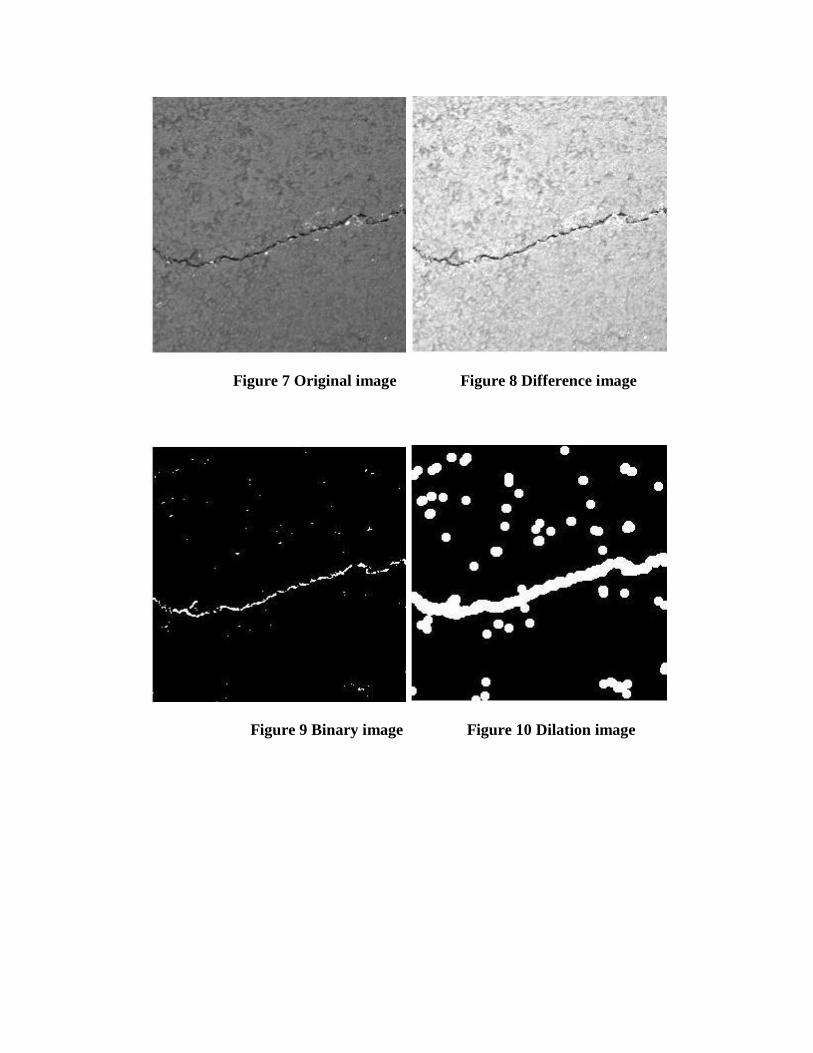
Figure 7 Original image Figure 8 Difference image
Figure 9 Binary image Figure 10 Dilation image

Figure 11 Erosion image Figure 12 Filtering image
Figure 13 Connecting image Figure 14 Median filter image

5. Conclusions
This project was an initial phase to design a framework for a prototype system that would
automate the pavement condition inspection though the use of digital imaging technology. The
researchers were able to achieve the objectives of the project. A new algorithm for extraction of
both transversal and horizontal cracks from pavement images has been developed as part of this
project. The first step of the developed algorithm involves pre-processing, which consists of
enhancement, thresholding, and morphological operations using dilation and erosion to eliminate
the remaining noise. One of the major components of the algorithm is the determination of the
break points and their connection for extraction of the crack features. The break points could
appear as a single or multiple points. This will in turn determine an appropriate search area in
each case. After finding the break points, a depth-first searching method is devised to connect
the break points within the search area. Simulation results demonstrate that the method can
effectively and efficiently extract the crack features from the pavement images. Future work
includes the calculation of the length and width of the cracks as well as detection and
quantification of other surface distresses. Subsequent phase(s) of this project will further
improve the accuracy and practicality of the automated inspection process and bring the
prototype system from the proof-of-concept stage to a functioning demonstrable system.

References [1] Newland D. E. “Wavelet analysis of vibration” Journal of vibration and acoustics. Vol.
116, pp. 409-416, 1994.
[2] Q. Wang, X. Deng. “Damage detection with spatial wavelets” International journal of
solids and structures. Vol. 36, pp3443-3468, 1999.
[3] S. T. Quek, Q. Wang, L. Zhang and K. K. Ang. “Sensitivity analysis of crack detection in
beams by wavelet technique” International journal of mechanical sciences. Vol. 43, No.
12, December, 2001.
[4] J. C. Hong, Y. Y. Kim, H. C. Lee and Y. W. Lee. “Damage detection using the Lipschitz
exponent estimated by the wavelet transform: applications to vibration modes of a beam”
International journal of solids and structures. Vol. 39, No. 7, April, 2002.
[5] E. Douka, S. Loutridis and A. Trochidis. “Crack identification in plates using wavelet
analysis” Journal of Sound and Vibration. Vol. 270, No. 1-2, February, 2004.
[6] Q. Q. Li and X. L. Liu. “A model for segmentation and distress statistic of massive
pavement images based on multi-scale strategies” The International Archives of the
Photogrammetry, Remote Sensing and Spatial Information Sciences. Vol. 37, Part B5.
2008.
[7] S. K. Sinha. “Automated condition assessment of buried pileline using computer vision
techniques” The 16th National Convention of Computer Engineers held at Patna.
December 2001.
[8] L. J. Hadjileontiadis, E. Douka and A. Trochidis. “Crack detection in beams using
kurtosis” Computer & Structures. Vol. 83, No. 12-13, May, 2005.
[9] H. D. Cheng, Jim-Rong Chen, Chris Glazier, and Y. G. Hu. “Novel approach to pavement
cracking detection based on fuzzy set theory” Journal of Computing in Civil
Engineering. Vol. 13, No. 4, October, 1999.
[10] Y. Huang and B. Xu. “Automatic inspection of pavement cracking distress” Journal of
Electronic Imaging. Vol. 15, 013017 February, 2006.
[11] Rolf Adams. “Radial decomposition of discs and spheres” Graphical Models and Image
Processing. Vol. 55, No. 5, pp. 325-332. September 1993.
[12] Rein Van Den Boomgaard and Richard Van Balen. “Methods for fast morphological
image transforms using bitmapped binary images” Graphical Models and Image
Processing. Vol. 54, No. 3, pp. 252-258. May 1992.

Appendix Matlab Implementation
1. Practical Experiment
The first step implemented is that of converting the RGB (i.e. the color image) as shown in
Fig A1 to a gray scale image. This conversion is required because Matlab is unable to
perform certain operations on a color image. For converting a color image to a gray scale
image, we firstly read the image and then perform the required operation using the function
rgb2gray. The function used for effectively reading an image in Matlab is imread.
1.1 Reading the image:
I = imread('pic9237.jpg');
figure; imshow(I);
title('Original Image');
1.2 Gray-Scale Conversion:
J = rgb2gray(I);
figure;
imshow(J);
title('gray scale image');
Once the image is converted to gray-scale as shown in Fig A2, our aim is to extract the
maximum crack features from the image. For this purpose we need to enhance the image to
make the cracks prominently visible. This is implemented by using the Histogram
Equalization method. The Matlab function used for this purpose is histeq. This function
enhances the contrast of images by transforming the values in the intensity image, or the
values in the colormap of an indexed image, so that the histogram of the output image
approximately matches a specified histogram.
1.3 Histogram Equalization:
Y = histeq(J);
figure;

imshow(Y);
title('Histogram Equalisation Image');
After the image has been enhanced as shown in Fig A3, we apply a filter to the image in
order to remove any noise from the image. For this purpose we have used the adaptive
filtering method. The Matlab function used is wiener2. The wiener2 function applies a
Wiener filter to an image adaptively, tailoring itself to the local image variance. Where the
variance is large, wiener2 performs little smoothing. Where the variance is small, wiener2
performs more smoothing.
This approach often produces better results than linear filtering. The adaptive filter is more
selective than a comparable linear filter, preserving edges and other high-frequency parts of
an image. In addition, there are no design tasks; the wiener2 function handles all preliminary
computations and implements the filter for an input image. The resultant filtered image is as
shown in Fig A4.
1.4 Adaptive Filtering:
K = wiener2(Y,[5 5]);
figure; imshow(Y);
title('filtered image');
RESULTS:

Fig A1. Original Image(Color Image)

Fig A2. Gray-Scale Image

Fig A3. Enhanced Image by Histogram Equalization Method

Fig A4. Filtered Image using Adaptive Filtering

2. Correcting Non-Uniform Illumination
While processing images using Morphological operations, the images need to have a uniform
illumination. Images with non-uniform illumination do not provide required results and can be
misleading. In order to obtain uniform background illumination, the following three steps need to
be followed. (However the ROI processing has not been considered as there not good papers
stating the procedure for processing an image for ROI. Secondly, the Morphological operations
have been used, which takes care of ROI and by using Otsu‟s technique of thresholding we can
obtain the same result as we would have obtained after ROI processing.)
1) Use Morphological Opening to Estimate the Background. The function mainly used for
this purpose is strel (structuring element).
SE = strel(shape, parameters) creates structuring element, SE, of the type specified by
shape. This function accepts various shapes like those of disc, line, diamond, octagon,
rectangle, square, etc.
background = imopen(J,strel('disk',15));
2) We can observe the non-uniform illumination in the image by displaying the non-
uniformity as a surface by approximating the background illumination. This is observed
from Fig A5.
figure, surf(double(background(1:8:end,1:8:end))),zlim([0 255]);
set(gca,'ydir','reverse');
3) Subtract the Backround Image from the Original Image. This step mainly subtracts the
background estimated by us in the previous step from the original image.
I2 = imsubtract(J,background);
figure;
imshow(I2);

2.1 Enhancing the Image:
The corrected image needs to be enhanced in order to make the features distinct and
prominent. The function used for this purpose is imadjust. This increases the contrast of the
output image.
I3 = imadjust(I2);
figure;
imshow(I3);
2.2 Thresholding:
Otsu‟s method is used for the purpose of thresholding. The graythresh function uses Otsu's
method, which chooses the threshold to minimize the intraclass variance of the black and white
pixels.
level = graythresh(I) computes a global threshold (level) that can be used to convert an intensity
image to a binary image with im2bw. level is a normalized intensity value that lies in the range
[0, 1].
level = graythresh(I3);
BW = im2bw(I3,level);
figure; imshow(BW);
title('thresholded image');

Fig A5. Background Approximation as a Surface


