
REVIEW
A review of refinery complexity applications
Mark J. Kaiser1
Received: 21 June 2016 / Published online: 4 January 2017
� The Author(s) 2017. This article is published with open access at Springerlink.com
Abstract Refinery complexity quantifies the sophistication
and capital intensity of a refinery and has found widespread
application in facility classification, cost estimation, sales
price models, and other uses. Despite the ubiquity and
widespread use of refining complexity, however, surprisingly
little material has been written on its applications. The pur-
pose of this review is to describe the primary applications of
refinery complexity and some recent extensions. A secondary
purpose of this review is to provide a framework that unifies
complexity applications and suggests avenues for future
research. Examples illustrate the applications considered.
Keywords Cost estimation � Functional complexity �Inverse problem � Replacement cost � Refineryclassification � Sales price models
1 Introduction
A refinery is an industrial plant where crude oil and other
feedstocks are processed into petroleum products. The
main principle of refining is to separate and improve the
hydrocarbon compounds that constitute crude oil to pro-
duce saleable products which satisfy regulatory require-
ments. A refinery is comprised of three main sections—
separation, conversion, and finishing—and each section
contains one or more process units that apply various
combinations of temperature, pressure, and catalyst to
perform their function.
All modern refineries have distillation units that perform
separation, but not all refineries perform conversion and
finishing operations. There are a dozen or so main process
operations in modern refining (Table 1), and for each
process, several technologies have been developed over the
past 150 years (Table 2). Different technologies involve
different trade-offs between operating and capital cost,
reliability and maintenance requirements (Schobert 2002;
Parkash 2003; Raseev 2003; Meyers 2004; Gary et al.
2007; Riazi et al. 2013).
1.1 Separate, convert, finish
Crude oil consists of hundreds of different types of
hydrocarbon molecules. Before processing, all refiners
physically separate crude oil into molecular weight ranges
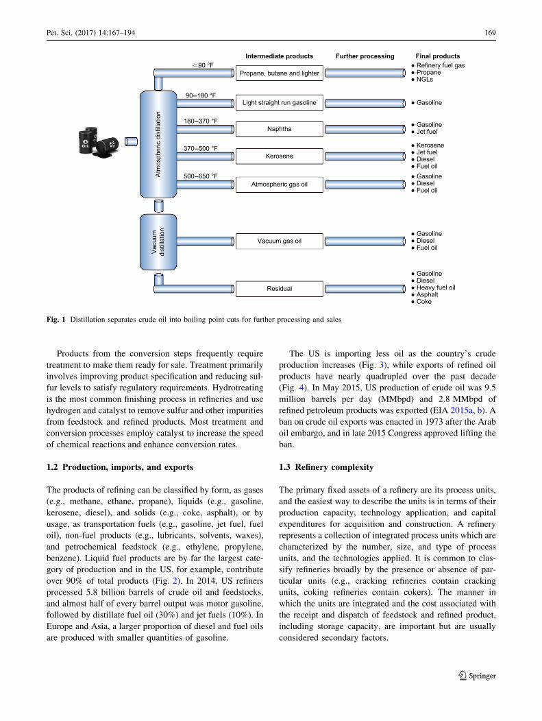
by boiling point using a distillation tower (Fig. 1). The
longer the carbon chain, the higher the temperature the
hydrocarbon compounds will boil. ‘‘Cuts’’ of similar boil-
ing point compounds are processed to allow the conversion
steps to operate efficiently. Processes downstream of dis-
tillation take these cuts, and using various chemical and
physical operations, improve and change the physical
properties of molecules which are subsequently blended for
fuels and other products (Speight 1998).
The conversion units in a modern refinery include
thermal cracking, catalytic cracking, hydrocracking and
coking. Thermal cracking was the first technology used to
increase gasoline production in 1913, but has been largely
replaced by more efficient processes. Conversion units are
expensive to build and operate and represent a major
investment decision, but once installed significantly extend
refinery flexibility and capability.
& Mark J. Kaiser
1 Center for Energy Studies, Louisiana State University,
Energy Coast and Environment Building, Baton Rouge,
LA 70803, USA
Edited by Xiu-Qin Zhu
123
Pet. Sci. (2017) 14:167–194
DOI 10.1007/s12182-016-0137-y

Table 1 Refining production process technologies. Source: OGJ
Process operation Technology
Coking Fluid coking, delayed coking, other
Thermal process Thermal cracking, visbreaking
Catalytic cracking Fluid, other
Catalytic reforming Semiregenerative, cycle, continuous regeneration, other
Catalytic hydrocracking Distillate upgrading, residual upgrading, lube oil, other
Catalytic hydrotreating Pre-treatment of cat reformer feeds, other naphtha desulfurization, naphtha aromatics saturation,
kerosene/jet desulfurization, diesel desulfurization, distillate aromatics saturation, other
distillates, pre-treatment of cat cracker feeds, other heavy gas oil hydrotreating, residual
hydrotreating, lube oil polishing, post-hydrotreating of FCC naphtha, other
Alkylation Sulfuric acid, hydrofluoric acid
Polymerization/dimerization Polymerization, dimerization
Aromatics BTX, hydrodealkylation, cyclohexane, cumene
Isomerization C4 feed, C5 feed, C5, and C6 feed
Oxygenates MTBE, ETBE, TAME
Hydrogen production
Hydrogen recovery
Steam methane reforming, steam naphtha reforming, partial oxidation
Pressure swing adsorption, cryogenic, membrane, other
Table 2 Evolution of refining technologies. Source: OSHA (2005)
Year Process Purpose By-products
1862 Atmospheric distillation Produce kerosene Naphtha, tar, etc.
1870 Vacuum distillation Produce lubricants Asphalt, residual coker feedstocks
1913 Thermal cracking Increase gasoline Residual, bunker fuel
1916 Sweetening Reduce sulfur and odor Sulfur
1930 Thermal reforming Improve octane number Residual
1932 Hydrogenation Remove sulfur Sulfur
1932 Coking Produce gasoline basestocks Coke
1933 Solvent extraction Improve lubricant viscosity index Aromatics
1935 Solvent dewaxing Improve pour point Waxes
1935 Catalytic polymerization Improve gasoline yield and octane number Petrochemical feedstocks
1937 Catalytic cracking Higher octane gasoline Petrochemical feedstocks
1939 Visbreaking Reduce viscosity Increased distillate, tar
1940 Alkylation Increase gasoline octane and yield High-octane aviation gasoline
1940 Isomerization Produce alkylation feedstock Naphtha
1947 Fluid catalytic cracking Increase gasoline yield and octane Petrochemical feedstocks
1950 Deasphalting Increase cracking feedstock Asphalt
1952 Catalytic reforming Convert low-quality naphtha Aromatics
1954 Hydrodesulfurization Remove sulfur Sulfur
1956 Inhibitor sweetening Remove mercaptan Disulfides
1957 Catalytic isomerization Convert to molecules with high octane number Alkylation feedstocks
1960 Hydrocracking Improve quality and reduce sulfur Alkylation feedstocks
1974 Catalytic dewaxing Improve pour point Wax
1975 Residual hydrocracking Increase gasoline yield from residual Heavy residuals
168 Pet. Sci. (2017) 14:167–194
123
Products from the conversion steps frequently require
treatment to make them ready for sale. Treatment primarily
involves improving product specification and reducing sul-
fur levels to satisfy regulatory requirements. Hydrotreating
is the most common finishing process in refineries and use
hydrogen and catalyst to remove sulfur and other impurities
from feedstock and refined products. Most treatment and
conversion processes employ catalyst to increase the speed
of chemical reactions and enhance conversion rates.
1.2 Production, imports, and exports
The products of refining can be classified by form, as gases
(e.g., methane, ethane, propane), liquids (e.g., gasoline,
kerosene, diesel), and solids (e.g., coke, asphalt), or by
usage, as transportation fuels (e.g., gasoline, jet fuel, fuel
oil), non-fuel products (e.g., lubricants, solvents, waxes),
and petrochemical feedstock (e.g., ethylene, propylene,
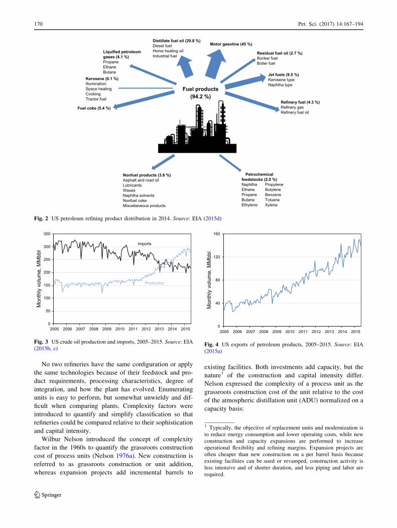
benzene). Liquid fuel products are by far the largest cate-
gory of production and in the US, for example, contribute
over 90% of total products (Fig. 2). In 2014, US refiners
processed 5.8 billion barrels of crude oil and feedstocks,
and almost half of every barrel output was motor gasoline,
followed by distillate fuel oil (30%) and jet fuels (10%). In
Europe and Asia, a larger proportion of diesel and fuel oils
are produced with smaller quantities of gasoline.
The US is importing less oil as the country’s crude
production increases (Fig. 3), while exports of refined oil
products have nearly quadrupled over the past decade
(Fig. 4). In May 2015, US production of crude oil was 9.5
million barrels per day (MMbpd) and 2.8 MMbpd of
refined petroleum products was exported (EIA 2015a, b). A
ban on crude oil exports was enacted in 1973 after the Arab
oil embargo, and in late 2015 Congress approved lifting the
ban.
1.3 Refinery complexity
The primary fixed assets of a refinery are its process units,
and the easiest way to describe the units is in terms of their
production capacity, technology application, and capital
expenditures for acquisition and construction. A refinery
represents a collection of integrated process units which are
characterized by the number, size, and type of process
units, and the technologies applied. It is common to clas-
sify refineries broadly by the presence or absence of par-
ticular units (e.g., cracking refineries contain cracking
units, coking refineries contain cokers). The manner in
which the units are integrated and the cost associated with
the receipt and dispatch of feedstock and refined product,
including storage capacity, are important but are usually
considered secondary factors.
<90 °F
90-180 °F
Propane, butane and lighter
Intermediate products
Atm
osph
eric
dis
tilla
tion
Vac
uum
dist
illat
ion
Further processing Final products● Refinery fuel gas● Propane● NGLs
● Gasoline
● Gasoline● Jet fuel
● Kerosene● Jet fuel● Diesel● Fuel oil● Gasoline● Diesel● Fuel oil
● Gasoline● Diesel● Fuel oil
● Gasoline● Diesel● Heavy fuel oil● Asphalt● Coke
Light straight run gasoline
Naphtha
Kerosene
Atmospheric gas oil
Vacuum gas oil
Residual
180-370 °F
370-500 °F
500-650 °F
Fig. 1 Distillation separates crude oil into boiling point cuts for further processing and sales
Pet. Sci. (2017) 14:167–194 169
123
No two refineries have the same configuration or apply
the same technologies because of their feedstock and pro-
duct requirements, processing characteristics, degree of
integration, and how the plant has evolved. Enumerating
units is easy to perform, but somewhat unwieldy and dif-
ficult when comparing plants. Complexity factors were
introduced to quantify and simplify classification so that
refineries could be compared relative to their sophistication
and capital intensity.
Wilbur Nelson introduced the concept of complexity
factor in the 1960s to quantify the grassroots construction
cost of process units (Nelson 1976a). New construction is
referred to as grassroots construction or unit addition,
whereas expansion projects add incremental barrels to
existing facilities. Both investments add capacity, but the
nature1 of the construction and capital intensity differ.
Nelson expressed the complexity of a process unit as the
grassroots construction cost of the unit relative to the cost
of the atmospheric distillation unit (ADU) normalized on a
capacity basis:
Fuel coke (5.4 %)
Kerosene (0.1 %)IlluminationSpace heatingCookingTractor fuel
Residual fuel oil (2.7 %)
Motor gasoline (45 %)
Bunker fuelBoiler fuel
Distillate fuel oil (29.8 %)
Fuel products(94.2 %)
Diesel fuelHome heating oilIndustrial fuel
Nonfuel products (3.8 %)Asphalt and road oilLubricantsWaxesNaphtha solventsNonfuel cokeMiscellaneous products
Petrochemicalfeedstocks (2.0 %)NaphthaEthanePropaneButaneEthylene
PropyleneButyleneBenzeneTolueneXylene
Jet fuels (9.5 %)Kerosene typeNaphtha type
Refinery fuel (4.3 %)Refinery gas Refinery fuel oil
Liquified petroleumgases (4.1 %)PropaneEthaneButane
Fig. 2 US petroleum refining product distribution in 2014. Source: EIA (2015d)
0
50
100
150
200
250
300
350
2005 2006 2007 2008 2009 2010 2011 2012 2013 2014 2015
Mon
thly
vol
ume,
MM
bbl
Imports
Production
Fig. 3 US crude oil production and imports, 2005–2015. Source: EIA(2015b, c)
0
40
80
120
160
2005 2006 2007 2008 2009 2010 2011 2012 2013 2014 2015
Mon
thly
vol
ume,
MM
bbl
Fig. 4 US exports of petroleum products, 2005–2015. Source: EIA(2015a)
1 Typically, the objective of replacement units and modernization is
to reduce energy consumption and lower operating costs, while new
construction and capacity expansions are performed to increase
operational flexibility and refining margins. Expansion projects are
often cheaper than new construction on a per barrel basis because
existing facilities can be used or revamped, construction activity is
less intensive and of shorter duration, and less piping and labor are
required.
170 Pet. Sci. (2017) 14:167–194
123

CFðUnit) ¼ CostðUnitÞ=CapacityðUnitÞCostðADU)/CapacityðADU)
Nelson applied the unit complexity factor to describe the
complexity and sophistication of a refinery. Each process
unit of a refinery is assigned a complexity factor via ref-
erence to projects constructed in the region at similar times,
and the sum of the complexity factors weighted by the unit
capacity relative to distillation capacity defines the com-
plexity index of the refinery at a point in time:
CI Refineryð Þ ¼X CapacityðUnitÞ
CapacityðADU) � CFðUnit)
1.4 Applications
Complexity indices quantify refinery complexity and have
been used in many different ways and for many different
purposes (Fig. 5). The more complex the refinery, the more
capital was invested to achieve its configuration, and
therefore, the greater the cost to insure and/or replace the
process units. Hence, refinery complexity is frequently
used by underwriters in determining premiums. Larger
refineries (refineries with greater distillation capacity) are
not necessarily more complex than smaller refineries, but a
refiner’s conversion capacity, that is, its cracking and
coking capacity, tend to be correlated to complexity,
illustrating how complexity may enter correlation studies.
Sophisticated refineries are more expensive to build
relative to simple refineries and should transact at a pre-
mium, for all things equal, because they consist of more
valuable assets, provide higher yields of more valuable
products, and generate greater margins. Complexity indices
are frequently used in sales price and replacement cost
models in appraisal studies, and derived measures such as
complexity barrels are frequently used in valuation and by
credit rating agencies.
1.5 Outline
The outline of this paper is as follows. We begin by
defining an ideal refinery and the variables and notation
employed throughout the paper. Complexity factors and
cross factors are introduced, and the methodologies used in
their measurement are reviewed. Complexity indices dif-
ferentiate refinery type and complexity classes are descri-
bed along with a snapshot of US statistics circa 2014. The
refinery complexity equation is used to quantify changes in
complexity index for changes in capacity and complexity
factor and is used to visually illustrate basic relations.
The relation between complexity, yields, and margins
are discussed, and applications to cost estimation are
described. By using cost functions, more precise formula-
tions of complexity are introduced and compared with the
traditional statistical approach. Using the complexity
equation, refinery complexity is more precisely described
in terms of its average and variance. Spatial complexity
generalizes the complexity index at geographic scales, and
application of complexity to replacement cost and sales
price models are illustrated.
Refinery complexity is commonly used as a correlating
variable in empirical studies, and complexity barrels rep-
resent one of the most popular uses of complexity that
combine distillation capacity and complexity and enjoys
widespread use by credit rating agencies when evaluating
corporate debt. The review concludes by formulating and
solving on inverse problem, where complexity factors are
inferred from a set of refinery complexity indices based on
the solution of a linear system of equations. The solution to
the inverse problem allows an analyst to infer the com-
plexity factors used in an assessment under particular
conditions if those factors are not provided.
2 Ideal refinery
A refinery R at time t is composed of n ? 1 process units
(U0, U1, …, Un) with charge or production capacities (Q0,
Q1, …, Qn) that depend on the unit type (Fig. 6). Process
unit U0 is designated as atmospheric distillation and Q0
denotes distillation capacity. Charge capacity is the liquid
volume of the crude that is fed to the process unit, while
production capacity refers to the barrels of product pro-
duced and both are expressed in barrels per stream day
(bpsd) or barrels per calendar day (bpd).2 In gas processing
and hydrogen plants, million cubic feet per day (MMcfd) of
Inverseproblem
Refineryclassification
Complexityequation
Yield &Margins
Costestimation
Functionalcomplexity
Complexitymoments
Spatialcomplexity
Replacementcost
Sales pricemodels
Correlations
Complexitybarrels
Refinerycomplexity
Fig. 5 Applications of refinery complexity vary widely
2 A barrel per stream day is the nameplate (design) capacity of a unit.
A barrel per calendar day represents the typical throughput capacity
taking into account downtime and related factors. Normally, calendar
day barrels range between 85% and 95% stream day barrels.
Pet. Sci. (2017) 14:167–194 171
123

gas are the base units; for solid coke and sulfur processing,
long tons are applied. Internationally, cubic meters and
metric tonnes are commonly employed in measurements.
The grassroots construction cost of unit Ui of capacity
Qi is denoted Ci(Qi) = C(Ui, Qi) and is always referenced
with respect to a specific project, time, and location. Pro-
ject characteristics, time, and location differences translate
to differences in the capital cost of construction which
requires adjustment and normalization before processing
with other cost data. Each process unit is described by a
complexity factor CFi, i = 1, …, n, and by definition, the
complexity factor of atmospheric distillation is one,
CF0 = 1. Complexity factors are derived measures based
on an empirical evaluation of cost data.
3 Complexity factors
3.1 Nelson complexity
Nelson defined the complexity factor of a process unit as
the cost of the unit relative to the cost of atmospheric
distillation normalized on a capacity basis:
CFi ¼ CF Uið Þ ¼ CF Ui;U0ð Þ ¼ CðUi;QiÞ=Qi
CðU0;Q0Þ=Q0
For example, if a 20,000 bpsd atmospheric distillation
unit in Houston, Texas, cost $5 million to construct in
1960, and a 2500 bpsd delayed coking unit cost $3 million
to construct in Lake Charles, Louisiana, in 1961, then the
complexity factor for delayed coking circa 1960 in the US
Gulf Coast (USGC) would be approximately five:
CFðDelayed CokingÞ ¼ $3 million=2500 bpsd
$5 million/20;000 bpsd¼ 4:8
In other words, the cost to construct one barrel of a 2500
bpsd delayed coker in the USGC circa 1960 was about five
times more expensive per barrel than the cost to build a
20,000 bpsd atmospheric distillation unit.
Two projects are not necessarily representative of
regional trends, and to increase confidence in the results
data collection should be expanded to ensure that a variety
of sizes, locations, and technologies are considered in
evaluation. Unfortunately, since multiple process units are
not frequently built in the same region or using the same
technologies, and because of confidentiality concerns in
contract negotiation, significant constraints exist in data
collection and the ability to provide reliable statistics on
complexity factors.
3.2 Measurement
Nelson published a list of complexity factors in the Oil &
Gas Journal (OGJ) for the major process units in the 1960s
(Nelson 1976a, b, 1977), which was later updated by Farrar
(1985, 1989) and continued to the present day in a com-
mercial format (Table 3). The last publicly reported USGC
complexity factors were in 1998, and so reference in this
paper to OGJ complexity factors refer to 1998 values.3
From 1961 to 1972, the complexity factors of vacuum
distillation, thermal cracking/visbreaking, and catalytic
hydrotreating were reported as two, indicating that during
this time, grassroots construction costs were about twice
the cost of a barrel of atmospheric distillation. Isomeriza-
tion capacity was three times as expensive as distillation,
catalytic reforming and hydrorefining four times as
expensive, and so on. Aromatics were reported as the most
expensive technology on a per barrel basis, and unlike the
other units, its complexity factor has declined. Complexity
factors for lubes, oxygenates, hydrogen, and asphalt units
were added in later years.
3.3 Complexity cross factor
Complexity factors are normalized with respect to atmo-
spheric distillation since atmospheric distillation is usually
Complexity factor, CFi
Ui
Charge capacity, Qi Production capacity, Qi
i=0
n
CI(R) = ∑ CFi = 1 +∑ CFi
Qi
Q0 i=0
n Qi
Q0
⎧⎨⎩
⎫⎬⎭
R =U0, U1, …, Un
Q0, Q1, …, Qn
Fig. 6 Refinery is described by its process units Ui and their charge
or production capacity Qi
3 OGJ complexity factors for most of the process units have not
changed significantly over several decades, either because construc-
tion cost did not change, or more likely, the cost data was not updated.
OGJ complexity factors available for purchase closely follow 1998
values, and no documentation is provided on cost data collected or
used.
172 Pet. Sci. (2017) 14:167–194
123

the cheapest process unit to build and has the greatest
throughput capacity. However, it is obvious that com-
plexity factors can be defined with respect to any two
process technologies, for example, hydrotreating or cat-
alytic cracking, in what we refer to as complexity cross
factors, or more simply cross factors.
The complexity cross factor for process unit Ui with
respect to unit Uj is defined as the normalized construction
cost per barrel for the respective units:
CF Ui;Uj
� �¼ CðUi;QiÞ=Qi
CðUj;QjÞ=Qj
Cross factors can be inferred from known complexity
factors, if available, since the distillation normalization
cancels out in the numerator and denominator terms:
CF Ui;Uj
� �¼ CFðUiÞ
CFðUjÞ
Conversely, if cross factors are available, complexity
factors can be inferred via the relation:
CFðUi;UjÞCFðUk;UjÞ
¼ CFðUiÞCFðUkÞ
3.4 Uncertainty
If process units were built frequently and reported their
construction cost consistently using standardized cost cat-
egories and accounting, complexity factors could be com-
puted with a high degree of reliability and would be subject
to minimal uncertainty and measurement bias, but because
units are not built frequently or in the same region or time
or with the same technologies or capacities, and because
cost data are rarely publicly available, the sample sets from
which complexity factors are computed are often small,
heterogeneous, and of low quality. Reliable cost data
therefore needs to be processed carefully, adjusted and
normalized prior to evaluation, with a clear understanding
of the inherent limitations of the analysis. Since only small
sample sets are available, small data analysis techniques
are applied, and uncertainty levels are expected to be high.
Example
Six USGC grassroots projects completed in 2010–2012
report construction cost ranging from $923/bpd for distil-
lation to $21,429/bpd for delayed coking (Table 4). Based
on this sample, complexity factors are computed to be 23
for delayed coking, 22 for VGO hydrocracking, 10 for
catalytic reforming, 8 for diesel hydrotreating, and 6 for
gasoline desulfurization, about two to four times greater
than the 1998 OGJ complexity factors. Cross factors for the
sample data and OGJ factors indicate a slightly smaller
range of variation (Table 5).
4 Refinery complexity
Refinery complexity quantifies the type of process units in
a refinery and their capacity relative to atmospheric dis-
tillation. Each process unit is assigned a complexity factor,
Table 3 Nelson’s complexity factors for refining operations. Source:OGJ
1961–1972 1989 1998
Atmospheric distillation 1 1 1
Vacuum distillation 2 2 2
Thermal operations
Thermal cracking, visbreaking 2 2 2.75
Delayed coking 5 5.5 6
Catalytic cracking 5.5 5.5 6
Catalytic reforming 4 5 5
Catalytic hydrocracking 6 6 6
Catalytic hydrorefining 4 3 3
Catalytic hydrotreating 2 1.7 2
Alkylation 9 11 10
Polymerization/dimerization 9 9 10
Aromatics 40–70 20 15
Isomerization 3 3 15
Lubes 10
Oxygenates 10
Hydrogen (MMcfd) 1
Asphalt 1.5
Table 4 Sample grassroots construction projects for US Gulf Coast, 2010–2012. Source: Industrial Information (2014)
Capacity,
Mbpd
Cost,
$ million
Unit cost,
$/bpd
CF Sample CF/
OGJ CF
Atmospheric distillation 325 300 923 1 1.0
Delayed coker 28 600 21,429 23 3.8
Catalytic reformer 55 500 9524 10 2.0
VGO hydrocracker 50 1000 20,000 22 4.0
Diesel hydrotreater 45 320 7111 8 4.0
Gasoline desulfurization 8 30 3750 4 2.0
Pet. Sci. (2017) 14:167–194 173
123

CFi, which is multiplied by the unit capacity Qi relative to
distillation capacity Q0, and when summed over all the
process units defines the complexity index CI(R) of the
refinery:
CIðRÞ ¼Xn
i¼0
Qi
Q0
CFi ¼ 1þXn
i¼1
Qi
Q0
CFi;
All process units of the refinery are part of the evalua-
tion, and if petrochemical facilities such as steam crackers
(olefins plant), cyclohexene, cumene, ammonia, and
methanol synthesis are present, these should be included.
Refinery configuration and process flows do not enter the
evaluation nor is the number of units (redundancy), vin-
tage, or specific technologies part of the computation.
Using the complexity index of a process unit, CI(Ui), the
refinery complexity is computed as the sum of the com-
plexity indices of its units:
CIðRÞ ¼ 1þXn
i¼1
CIðUiÞ;
where CI(Ui) = (Qi/Q0)CFi.
Example
In 2015, Kern Oil & Refining’s Bakersfield, California,
refinery reported 25 Mbpd atmospheric distillation capac-
ity, 3 Mbpd catalytic reforming capacity, and 13 Mbpd
hydrotreating capacity. Using the 1998 OGJ complexity
factors, the refining complexity is computed as
CI Bakersfieldð Þ ¼ 25
25ð1Þ þ 3
25ð5Þ þ 13
25ð2Þ ¼ 2:6
Example
In 2014, PBF Energy’s Delaware City, Delaware, refinery
reported 190 Mbpd atmospheric distillation capacity, 102
Mbpd vacuum distillation, 82 Mbpd fluid catalytic crack-
ing, 47 Mbpd fluid coking, and 18 Mbpd hydrocracking
capacity. Hydrotreaters process straight run naphtha, die-
sel, and middle distillates with 160 Mbpd total capacity,
and there is 16 Mbpd polymerization, 11 Mbpd alkylation,
and 6 Mbpd isomerization capacity. Hydrogen production
is via steam methane reforming. Refinery complexity circa
2014 computed using 1998 OGJ complexity factors is 12.9
(Table 6).
Table 5 Complexity cross
factor comparison for US Gulf
Coast, 2010–2012.
USGC sample, 2010–2012 OGJ, 1998
1 2 3 4 5 6 1 2 3 4 5 6
1. Atmospheric distillation 1.0 1.0
2. Delayed coker 23.2 1.0 6.0 1.0
3. Catalytic reformer 9.8 0.4 1.0 5.0 0.8 1.0
4. VGO hydrocracker 21.7 0.9 2.2 1.0 5.5 0.9 1.1 1.0
5. Diesel hydrotreater 7.7 0.3 0.8 0.4 1.0 2.0 0.3 0.4 0.4 1.0
6. Gasoline desulfurization 4.1 0.2 0.4 0.2 0.5 1.0 2.0 0.3 0.4 0.4 1.0 1.0
Based on data in Table 4
Table 6 PBF Energy’s
Delaware City, Delaware,
refinery complexity (2014)
Capacity, Mbpd ADU capacity, % CF CI
Atmospheric distillation 190 100 1 1.0
Vacuum distillation 102 54 2 1.1
Fluid catalytic cracking 82 43 6 2.6
Hydrotreating 160 84 2 1.7
Hydrocracking 18 9 6 0.6
Catalytic reforming 43 23 5 1.1
Benzene/Toluene extraction 15 8 15 1.2
Butane isomerization 6 3 15 0.5
Alkylation 11 6 10 0.6
Polymerization 16 8 10 0.8
Fluid coking 47 25 6 1.5
Hydrogen (MMcfd) 62 33 1 0.3
Refinery complexity 12.9
174 Pet. Sci. (2017) 14:167–194
123

5 Refinery classification
5.1 Categorization
In the US, refineries are commonly referred to as simple or
complex, or using more specific descriptors (Fig. 7).
Refineries with cracking and coking capacity are generally
referred to as ‘‘cracking’’ and ‘‘coking’’ refineries, respec-
tively, or as ‘‘complex’’ or ‘‘very complex’’ refineries, to
distinguish from ‘‘simple’’ refineries which do not have
such units. In Europe and elsewhere, it is common to refer
to complex refineries as ‘‘conversion’’ or ‘‘deep conver-
sion’’ refineries.
Simple refineries are often referred to as topping or
hydroskimming plants since they only split crude oil into
its main components and perform basic finishing opera-
tions. Topping facilities are basically just a distillation
tower, while hydroskimmers also contain reforming and
hydrotreating, and sometimes aromatics recovery units.
Simple refineries maintain a high straight run fuel oil
production and produce a high straight run fuel oil. Most
coking facilities have cracking capacity, but not all
cracking facilities have cokers. Coking refineries upgrade
most of the fuel oil to lighter products.
The terminology to distinguish refinery classes and the
complexity ranges employed are not universally recog-
nized, but the following names and thresholds are common:
Classification Name Complexity range
Very simple Topping \2
Simple Hydroskimming 2–5
Complex Cracking, conversion 5–14
Very complex Coking, deep conversion [14
Specialty Lube oils, asphalt [5
Integrated Petrochemical [10
Specialty refineries usually refer to lubricating and base
oil plants or asphalt refineries. Refineries integrated with
petrochemical facilities typically employ a large amount of
aromatics recovery and include cumene and cyclohexane
units, ammonia and methanol synthesis.
5.2 Topping refinery
A ‘‘topping’’ refinery relies entirely on distillation to sep-
arate cuts and is the simplest type of refinery that can be
built. Residuum is sold as a heavy fuel oil, and if vacuum
distillation is available, part of the residuum could be made
into asphalt. No additional processing occurs at topping
refineries, and much of the output stream is sold to other
refineries with additional processing capacity. Topping
refineries are usually built to prepare feedstocks for
petrochemical manufacture or for the production of
industrial fuels in remote areas. A large portion of the
production from topping refineries is straight run fuel oil.
A topping refinery has no conversion or finishing pro-
cesses, and its range of products is entirely dependent on the
characteristics of the crude oil. For example, a crude that
contains 25% gasoline boiling range molecules and 15%
diesel boiling range molecules will produce approximately
25% gasoline boiling range cuts and 15% diesel cuts in a
topping facility. A portion of the naphtha stream may be
suitable for low octane gasoline in some areas, but because
topping refineries do not have facilities for controlling product
sulfur levels, the gasoline products may not be suitable for
direct consumption and the refinery probably cannot produce
ultralow sulfur fuels unless the crude is light and sweet.
Example
The Prudhoe Bay Crude Oil Topping Unit (COTU), owned
and operated by ConocoPhillips Alaska Inc., maintained
16,000 bpsd (15,000 bpd) distillation capacity in 2014 to
provide arctic heating fuel (AHF) for the Endicott/Badami
field operations in the North Slope of Alaska. The COTU
consists entirely of two parallel atmospheric distillation
towers. Each plant heats the crude to approximately 550 �Fand distills off the AHF fraction. The AHF is sent to
storage tanks for use, and the remaining fluids are recom-
bined and re-injected back into the oil transfer line. Each
plant is capable of processing approximately 7000–8000
bpd of crude with production of 1200–1400 bpd of AHF.
Production of Jet A is done on a periodic batch basis. AHF
and Jet A are the only products of the unit and all pro-
duction is consumed on site.
Refinerycomplexity
Simple
Topping
Very simpleCI<2
Simple2≤CI<5
Complex5≤CI<14
Very complexCI≥14
Hydroskimmer Conversion(cracker)
Specialty
Integrated
Deep conversion(coker)
Complex
Fig. 7 Refinery classification including specialty and integrated
refinery and typical complexity ranges
Pet. Sci. (2017) 14:167–194 175
123

5.3 Simple refinery
Low-complexity refineries typically run light/sweet crude
oil and produce a high yield of low-quality products
(Fig. 8). Hydroskimmers make extensive use of hydrogen
treatment to clean up the naphtha and distillate streams to
satisfy regulatory specifications, and to pre-treat naphtha
feedstock to remove sulfur to avoid poisoning the reformer
catalyst. Reformers upgrade naphtha into high-octane
reformate to meet gasoline octane specification and provide
an important source of hydrogen4 for hydrotreating.
Reforming produces aromatics (e.g., benzene, toluene,
xylene) and some hydroskimmers employ aromatics
recovery units to separate out these high-value products for
sales to petrochemical plants.
Example
In 2015, Galp Energia’s 91.3-Mbpd Matosinhos refinery in
Portugal had vacuum distillation capacity of 16.4 Mbpd,
catalytic reforming capacity of 25.4 Mbpd, catalytic
hydrotreating capacity of 76.9 Mbpd, and aromatics
capacity of 17.3 Mbpd. Using OGJ complexity factors as a
proxy for international construction, the Matosinhos refin-
ery complexity is computed to be 7.3 (Table 7).
Galp Energia refer to their refinery as a hydroskimmer,
and although the complexity index exceeds the normal
cutoff of a ‘‘simple’’ US refinery, the classification is
appropriate since the facility does not contain any con-
version processes. Aromatics contribute about 40% of the
complexity score, and because the plant also produces
lubricants, base oils, and solvents, if located in the US the
refinery would be called a fuels-lubes plant.
5.4 Complex (conversion) refinery
Conversion processes carry out chemical reactions that
crack large, high-boiling point hydrocarbon molecules into
smaller, lighter molecules suitable for gasoline, jet fuel,
diesel fuel, petrochemical feedstocks, and other high-value
products. The primary conversion processes that perform
these operations are fluid catalytic cracking (FCC),
hydrocracking, and coking. Visbreaking is a thermal con-
version process similar to coking but is milder and rarely
Propane/butane 4 % Propane/butane
30 % Gasoline
34 % Distillate ● Diesel ● Heating oil ● Jet fuel
32 % Heavy fuel oil& other
Low octane gasoline & naphtha
Atm
osph
eric
dis
tilla
tion
Vac
uum
dist
illat
ion
High sulfur kerosene/jet fuel
High sulfur diesel/heating oil
High octane gasolineReformer
Distillatedesulfurizer
Low sulfur kerosene/jet fuel
Low sulfur diesel/heating oil
Gas oil
Heavy fuel oil/residul
Fig. 8 Schematic of a low-complexity refinery and typical product output
Table 7 Galp Energia’s
Matosinhos, Portugal, refinery
complexity (2014)
Capacity, Mbpd ADU capacity, % CF CI
Atmospheric distillation 91.3 100 1 1.0
Vacuum distillation 16.4 18 2 0.4
Catalytic reforming 25.4 28 5 1.4
Catalytic hydrotreating 76.9 84 2 1.7
Aromatics recovery 17.3 19 15 2.8
Refinery complexity 7.3
1998 OGJ complexity factors are used as a proxy for the international units in the calculation
4 Historically, many US refineries built before 1975 had their
reformers designed to be in hydrogen balance with the hydrotreaters.
Today, hydrogen requirements at US plants not satisfied by reforming
are produced primarily by steam methane reforming.
176 Pet. Sci. (2017) 14:167–194
123
used in the US anymore, but is still common in Europe and
other parts of the world where legacy units remain in
operation.
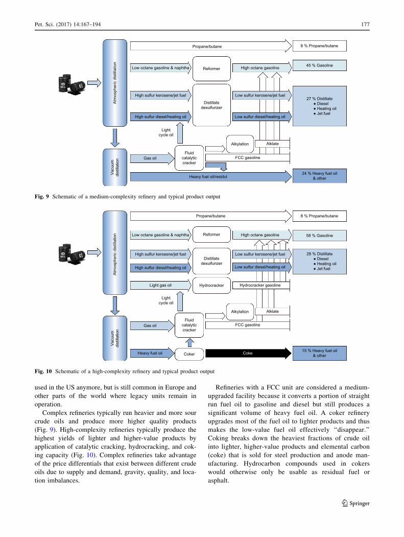
Complex refineries typically run heavier and more sour
crude oils and produce more higher quality products
(Fig. 9). High-complexity refineries typically produce the
highest yields of lighter and higher-value products by
application of catalytic cracking, hydrocracking, and cok-
ing capacity (Fig. 10). Complex refineries take advantage
of the price differentials that exist between different crude
oils due to supply and demand, gravity, quality, and loca-
tion imbalances.
Refineries with a FCC unit are considered a medium-
upgraded facility because it converts a portion of straight
run fuel oil to gasoline and diesel but still produces a
significant volume of heavy fuel oil. A coker refinery
upgrades most of the fuel oil to lighter products and thus
makes the low-value fuel oil effectively ‘‘disappear.’’
Coking breaks down the heaviest fractions of crude oil
into lighter, higher-value products and elemental carbon
(coke) that is sold for steel production and anode man-
ufacturing. Hydrocarbon compounds used in cokers
would otherwise only be usable as residual fuel or
asphalt.
Propane/butane 8 % Propane/butane
45 % Gasoline
27 % Distillate ● Diesel ● Heating oil ● Jet fuel
24 % Heavy fuel oil& other
Atm
osph
eric
dis
tilla
tion
Vac
uum
dist
illat
ion
High octane gasolineReformer
Distillatedesulfurizer
Lightcycle oil
Fluidcatalyticcracker
Low sulfur kerosene/jet fuel
Low sulfur diesel/heating oil
Low octane gasoline & naphtha
High sulfur kerosene/jet fuel
High sulfur diesel/heating oil
Gas oil
Heavy fuel oil/residul
Alkylation
FCC gasoline
Alklate
Fig. 9 Schematic of a medium-complexity refinery and typical product output
Propane/butane 8 % Propane/butane
58 % Gasoline
28 % Distillate ● Diesel ● Heating oil ● Jet fuel
15 % Heavy fuel oil& other
Atm
osph
eric
dis
tilla
tion
Vac
uum
dist
illat
ion
High octane gasolineReformer
Distillatedesulfurizer
Hydrocracker
Lightcycle oil
Fluidcatalyticcracker
Coker
Low sulfur kerosene/jet fuel
Low sulfur diesel/heating oil
Low octane gasoline & naphtha
Light gas oil
High sulfur kerosene/jet fuel
High sulfur diesel/heating oil
Gas oil
Heavy fuel oil
Alkylation
FCC gasoline
Alklate
Hydrocracker gasoline
Coke
Fig. 10 Schematic of a high-complexity refinery and typical product output
Pet. Sci. (2017) 14:167–194 177
123

The pressure of cracking and coking units almost always
indicates additional process technologies within the refin-
ery such as alkylation or polymerization units for con-
verting olefin streams to gasoline and petrochemical
blendstocks, aromatics, asphalt plants, sulfur recovery, and
hydrogen production.
Conversion capacity is a measure of a refinery’s con-
version units relative to atmospheric distillation. It is
defined as the ratio of a plant’s cracking and coking
capacity divided by atmospheric distillation capacity:
Conversion capacity ¼ Cracking capacityþ coking capacity
Atmospheric distillation capacity
Cracking includes thermal cracking, visbreaking, cat-
alytic cracking, and hydrocracking. The conversion
capacity of the most complex US refineries are generally
greater than 75%, and in some cases, can exceed 100%.
Refinery size is not correlated with conversion capacity.
Example
Pasadena Refining’s Pasadena, Texas, and Citgo Petro-
leum’s Corpus Christi, Texas, refineries have complexity
indices of 7.4 and 13.8, respectively (Table 8). Neither
facility has a hydrogen plant. The Corpus Christi refinery
has a greater percentage of more complex units as well as
greater hydrotreating capacity which is responsible for its
higher complexity index. At the Pasadena refinery, the
conversion capacity is 53% (=62/117), and at Corpus
Christ, the conversion capacity is 70% (=110/157).
Example
SK Group’s Ulsan 840-Mbpd refinery in South Korea has a
complexity index of 7.2 and is the third largest refinery in
the world circa 2014 with 147 Mbpd catalytic cracking and
45 Mbpd hydrocracking capacity. The conversion capacity
at Ulsan, however, is only 23% (=192/840), representing
low-upgrading capacity.
6 USA and world statistics
In 2014, world refining capacity was 90 MMbpd, and
approximately half of the 646 refineries were cracking
facilities, 35% were cokers, 10% were hydroskimmers, and
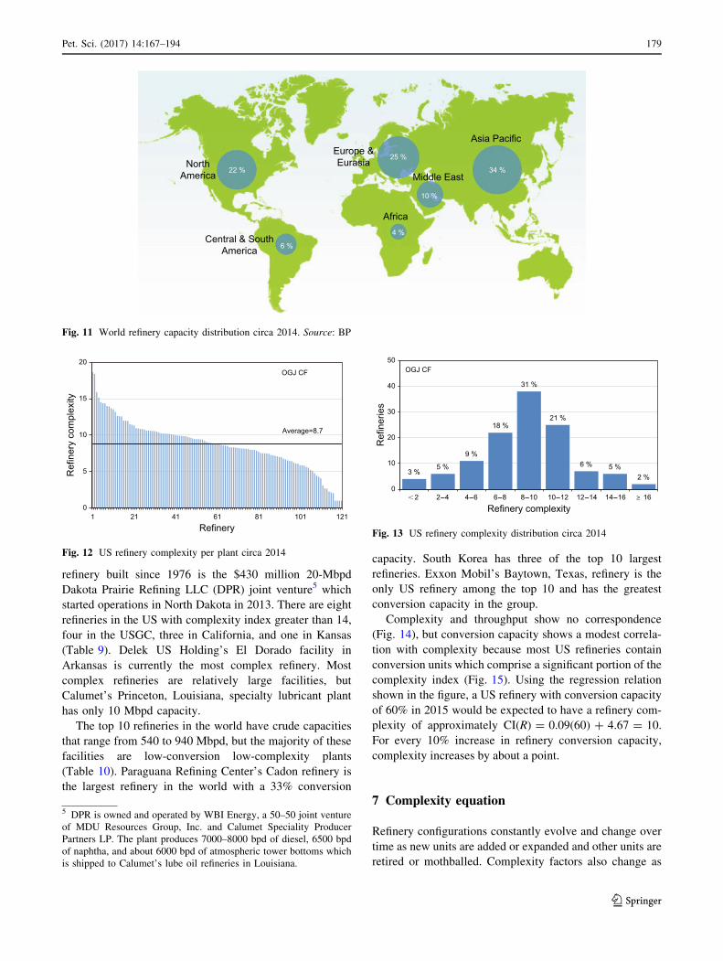
5% were topping plants (OGJ 2014). North America and
Europe held about a quarter of refining capacity each, fol-
lowed by the Middle East, Central and South America
(Fig. 11). The Asia–Pacific region, which includes Russia,
China, India, and Australia, held about a third of global
distillation capacity. In theUnited States, the vastmajority of
refineries are conversion facilities of medium-to-high com-
plexities. In Asia, theMiddle East, and South America, areas
that are experiencing rapid growth for gasoline demand and
light products, almost all new construction is conversion and
deep conversion facilities. In Europe, Japan, and Russia,
hydroskimming refineries are common, and in recent years
several have been shut down or under severe financial dis-
tress due to competition with newly built refineries.
In 2014, 122 refineries in the USA maintained 18.1
MMbpd distillation capacity with an average plant com-
plexity of 8.7 (Fig. 12). There were four refineries (3%)
with complexity index less than 2, 17 refineries (14%) with
complexity between 2 and 6, 96 refineries (70%) with
complexity between 6 and 12, and 15 refineries (13%) with
complexity greater than 12 (Fig. 13). Large variations in
complexity are due to local market requirements, devel-
opment pathways and consolidation trends, and of course,
diverse configurations across plants. About a third of US
refineries have complexity index greater than 10.
Most topping refineries are located in Alaska, but the
most recent topping plant and the first US greenfield
Table 8 Pasadena Refining’s Pasadena, Texas, and Citgo Petroleum’s Corpus Christi, Texas, refinery complexity (2013)
CF Pasadena (TX) CI Corpus Christi (TX) CI
Capacity,
Mbpd
ADU capacity,
%
Capacity,
Mbpd
ADU capacity,
%
Atmospheric distillation 1.0 117 100 1.0 157 100 1.0
Vacuum distillation 2.0 41 35 0.7 74 47 0.9
Delayed coking 6.0 12 10 0.6 38 24 1.4
Catalytic cracking 6.0 50 43 2.6 72 46 2.8
Catalytic reforming 5.0 20 17 0.9 45 29 1.4
Catalytic hydrotreating 2.0 44 38 0.8 148 95 1.9
Alkylation 10.0 11 9 0.9 18 12 1.2
Aromatics 15.0 – – – 30 19 2.9
Oxygenates 10.0 – – – 4 2 0.2
Refinery complexity 7.4 13.8
178 Pet. Sci. (2017) 14:167–194
123
refinery built since 1976 is the $430 million 20-Mbpd
Dakota Prairie Refining LLC (DPR) joint venture5 which
started operations in North Dakota in 2013. There are eight
refineries in the US with complexity index greater than 14,
four in the USGC, three in California, and one in Kansas
(Table 9). Delek US Holding’s El Dorado facility in
Arkansas is currently the most complex refinery. Most
complex refineries are relatively large facilities, but
Calumet’s Princeton, Louisiana, specialty lubricant plant
has only 10 Mbpd capacity.
The top 10 refineries in the world have crude capacities
that range from 540 to 940 Mbpd, but the majority of these
facilities are low-conversion low-complexity plants
(Table 10). Paraguana Refining Center’s Cadon refinery is
the largest refinery in the world with a 33% conversion
capacity. South Korea has three of the top 10 largest
refineries. Exxon Mobil’s Baytown, Texas, refinery is the
only US refinery among the top 10 and has the greatest
conversion capacity in the group.
Complexity and throughput show no correspondence
(Fig. 14), but conversion capacity shows a modest correla-
tion with complexity because most US refineries contain
conversion units which comprise a significant portion of the
complexity index (Fig. 15). Using the regression relation
shown in the figure, a US refinery with conversion capacity
of 60% in 2015 would be expected to have a refinery com-
plexity of approximately CI(R) = 0.09(60) ? 4.67 = 10.
For every 10% increase in refinery conversion capacity,
complexity increases by about a point.
7 Complexity equation
Refinery configurations constantly evolve and change over
time as new units are added or expanded and other units are
retired or mothballed. Complexity factors also change as
NorthAmerica
Central & SouthAmerica
Europe &Eurasia
Middle East
Africa
Asia Pacific
22 %
6 %
25 %
10 %
34 %
4 %
Fig. 11 World refinery capacity distribution circa 2014. Source: BP
0
5
10
15
20
1 21 41 61 81 101 121
Ref
iner
y co
mpl
exity
Refinery
Average=8.7
OGJ CF
Fig. 12 US refinery complexity per plant circa 2014
3 %5 %
9 %
18 %
31 %
21 %
6 % 5 %2 %
0
10
20
30
40
50
<2 2-4 4-6 6-8 8-10 10-12 12-14 14-16 ≥ 16
Ref
iner
ies
Refinery complexity
OGJ CF
Fig. 13 US refinery complexity distribution circa 2014
5 DPR is owned and operated by WBI Energy, a 50–50 joint venture
of MDU Resources Group, Inc. and Calumet Speciality Producer
Partners LP. The plant produces 7000–8000 bpd of diesel, 6500 bpd
of naphtha, and about 6000 bpd of atmospheric tower bottoms which
is shipped to Calumet’s lube oil refineries in Louisiana.
Pet. Sci. (2017) 14:167–194 179
123

technologies change, and the relative cost of construction
change. If the distillation capacity of a plant increases
holding all other process capacities and complexity factors
fixed, for example, refinery complexity will decrease since
the individual weight factors will decline, while if one or
more units are added or expanded for a given crude
capacity, refinery complexity will increase. Refinery
complexity will also change if complexity factors change
over time.
Refinery complexity is a function of the capacity vari-
ables (Q0, Q1, …, Qn) and complexity factors (CF0, CF1,
…, CFn) as expressed in the complexity equation:
Table 9 Most complex US refineries circa 2014. Source: OGJ (2014)
Company Location Capacity,
Mbpd
CI Conversion capacity,
%
Delek US Holdings Inc. El Dorado, AR 80 18.7 76
Total SA Port Arthur, TX 169 18.4 73
Calumet Lubricants Co. Princeton, LA 10 15.9 80
National Cooperative Refining Assoc. McPherson, KS 85 15.1 94
Phillips 66 Los Angeles, CA 139 14.5 85
Shell Oil Products, USA Martinez, CA 145 14.4 105
Valero Energy Corp. Corpus Christi, TX 205 14.4 77
Chevron Corp. Richmond, CA 257 14.0 90
1998 OGJ complexity factors used in the complexity index calculation
Table 10 World’s largest refineries circa 2014. Source: OGJ (2014)
Rank Company Location Capacity,
Mbpd
CI Conversion capacity,
%
1 Paraguana Refining Center Cardon/Judibana, Falcon, Venezuela 940 6.3 33
2 SK Innovation Ulsan, South Korea 840 7.2 23
3 GS Caltex Corp. Yeosu, South Korea 785 7.4 38
4 S-Oil Corp. Onsan, South Korea 669 7.7 29
5 Reliance Industries Ltd. Jamnagar, India 660 3.3 39
6 ExxonMobil Refining & Supply Co. Jurong/Pulau Ayer Chawan, Singapore 593 5.3 10
7 Reliance Petroleum Ltd. Jamnagar, India 580 6.7 54
8 ExxonMobil Refining & Supply Co. Baytown, Texas 561 10.2 57
9 Saudi Arabian Oil Co. Ras Tanura, Saudi Arabia 550 3.2 9
10 Formosa Petrochemical Co. Mailiao, Taiwan 540 7.0 42
1998 OGJ complexity factors used in the complexity index calculation
0
4
8
12
16
20
0 100 200 300 400 500 600 700
Ref
iner
y co
mpl
exity
Capacity, Mbpd
OGJ CF
Fig. 14 Refinery complexity and atmospheric distillation capacity of
US refineries (2014)
y = 0.09x + 4.67R
2 = 0.48
0
4
8
12
16
20
0 20 40 60 80 100 120
Ref
iner
y co
mpl
exity
Conversion capacity, %
OGJ CF
Fig. 15 Refinery complexity and conversion capacity of US refiner-
ies (2014)
180 Pet. Sci. (2017) 14:167–194
123

CIðRÞ ¼ CIðQ0;Q1; . . .;Qn;CF1;CF2; . . .;CFnÞ
¼Xn
i¼0
Qi
Q0
CFi ¼ 1þXn
i¼1
Qi
Q0
CFi
Clearly, refinery complexity is linear in Qi and CFi, and
nonlinear in Q0. The partial derivatives provide predictive
information on the shape of the complexity function, and
its sensitivity to parameter variation when one variable
changes and all other variables are held fixed (Fig. 16):
oCI
oQ0
¼ �1
Q20
Xn
i¼1
QiCFi
oCI
oQi¼ CFi
Q0
; i ¼ 1; 2; . . .; n
oCI
oCFi¼ Qi
Q0
; i ¼ 1; 2; . . .; n
8>>>>>>>>>><
>>>>>>>>>>:
Example
Silver Eagle Refining Inc.’s Woods Cross, Utah, refinery in
2014 had 6.25 Mbpd atmospheric distillation capacity, 6
Mbpd vacuum distillation, 2.2 Mbpd catalytic reforming,
6.2 Mbpd catalytic hydrotreating, and 1.2 Mbpd asphalt
production.
The refinery complexity equation as a function of
atmospheric distillation capacity is written:
CIðQ0Þ ¼ 1þ 6 Mbpd
Q0 MbpdCFVDU þ 2:2 Mbpd
Q0 MbpdCFCCR
þ 6:2 Mbpd
Q0 MbpdCFHT þ
1:2 Mbpd
Q0 MbpdCFASH
Using OGJ complexity factors for the process units
(CFVDU = 2, CFCCR = 5, CFHT = 2, CFASH = 1.5), the
refinery complexity relation simplifies as
CI(Q0) = 1 ? 37.2/Q0 (Fig. 17). For the refinery configu-
ration circa 2014 with 6.25 Mbpd distillation capacity, the
complexity index is 7.0, but if distillation capacity
increased to 9.25 Mbpd holding all the other units and
complexity factors fixed, the complexity index would be
5.0. As ADU capacity increases refinery complexity
decreases nonlinearly, which is related to the slope of the
relation. The slope of the complexity equation at any
capacity along the curve is determined by the first deriva-
tive, oCI/oQ0 = �37:2=Q20.
The refinery complexity equation for variable reformer
capacity holding all other process units and complexity
factors fixed is evaluated as:
CIðQCCRÞ ¼ 1þ 6ð2Þ6:25
þ 5QCCR
6:25þ 6:2ð2Þ
6:25þ 1:2ð1:5Þ
6:25
¼ 5:192 þ 0:8QCCR:
Increasing reformer capacity increases refinery complexity
linearly defined by the 0.8 slope of the equation (Fig. 17).
Similarly, holding all the process capacities fixed and
varying the complexity factor for one unit, say the asphalt
plant, the refinery complexity equation becomes
CI(CFASH) = 6.664 ? 0.192�CFASH and the slope of
complexity equation describes how changes in the asphalt
complexity factor change the complexity index. For
example, if the actual asphalt complexity factor was 4.5
instead of 1.5, the refinery complexity would be 7.5.
Ref
iner
y co
mpl
exity
Capacity, Mbpd
(Qi Variable; CFi , Q0 Fixed)
(Q0 Variable; CFi , Qi Fixed)
i=0
n
CI(R) = ∑ CFi Qi
Q0
Slope =CFi
Q0
Slope = - ∑Qi CFi 1
Q02
Fig. 16 Partial derivatives provide information on the shape of the
refinery complexity equation
10
8
6
4
2
05 7 9
ADU capacity, Mbpd
Ref
iner
y co
mpl
exity
11 13 15 17 19
Slope = - 37.2Q02
16
12
8
4
01 3
CCR capacity, Mbpd
Ref
iner
y co
mpl
exity
5 7 9
Slope = 0.8
(a) (b)
Fig. 17 Woods Cross, Utah, refinery complexity as a function of crude capacity and reforming capacity circa 2014
Pet. Sci. (2017) 14:167–194 181
123

8 Cost estimation
Complexity factors are derived from cost data and are
therefore useful in cost estimation, but to be an accurate
and reliable indicator of cost, they must be up-to-date and
representative for the region of interest. Rearranging the
complexity factor equation yields the cost estimation
relation:
CðUjÞ ¼CFi
CFj
Qi
QjCðUjÞ
The cost of a process unit is estimated using the relation
between complexity factors and capacities and the cost of a
known unit.
Example
A 325-Mbpd atmospheric distillation unit was built in
Texas in 2012 for $300 million. If the complexity factor of
hydrocracking is 22, then the cost to construct a 35-Mbpd
hydrocracker in Texas in 2012 is estimated to be $711
million:
C Hydrocrackerð Þ ¼ 22 35 Mbpdð Þ $300 million
325 Mbpd
� �
¼ $711 million
Example
A 57-Mbpd USGC hydrocracker cost $1000 million to
construct in 2012. If the complexity cross factor for the
hydrocracker and refiner is 2.2, the construction cost of a
40-Mbpd reformer built in the USGC in 2012 is estimated
to be $319 million:
C Reformerð Þ ¼ 1
2:2
� �$1000 million
57 Mbpd
� �40 Mbpdð Þ
¼ $319 million
Example
A 400-Mbpd coking refinery in Jieyang, China, is expected
to be completed in 2017–2018 (Table 11). The 60,000-bpd
catalytic cracking unit cost $406 million, and its normalized
construction cost is computed as $6766/bpd. Using this data
point and normalizing by the USGC complexity factors, the
total cost of the refinery is estimated at $6.6 billion, about
three-quarters of the $9 billion reported estimate. Differ-
ences between the estimated and expected total cost is due to
regional variation in the complexity factors and the first-
order approximation of the estimation equation.
9 Functional complexity
9.1 Cost function formulations
A more precise way to formulate complexity factors is to
process the sample data using cost functions, and then to
apply the cost functions at specified capacities, or to specify
the capacity interval of each unit and create the complexity
factor functional (Kaiser 2016). The cost data are the same in
all three approaches, of course, but how the data are processed
and evaluated are different, and consequently, the resultant
complexity factor values will also be different (Fig. 18).
In the traditional (statistical) approach to complexity
factors, the cost data are normalized by capacity via divi-
sion, and then statistical techniques are applied in pro-
cessing. The computations are easy to perform, but one of
the limitations of the method is the inability to account
directly for the impact of capacity on cost. There is no
‘‘control’’ in the data sample, and since we are not con-
trolling for capacity directly, its impact is unknown.
Capacity is not a control variable, but used as input data to
normalize the complexity factor.
In the reference capacity approach, the use of cost
functions improves the reliability and transparency of the
calculations and accounts for capacity variation, and since
capacity is required in the assessment, it improves speci-
ficity since this term must be specified. Complexity factors
at reference capacity (CFRC) specify ‘‘representative’’
capacities in the cost functions, but the data used in con-
structing cost functions span a wide spectrum of costs and
Table 11 Cost estimation at
the Jieyang, China, coking
refinery (2014)
Capacity,
Mbpd
Units,
#
CFRC Unit cost,
$/bpd
Total cost,
$million
Atmospheric
distillation
200,000 2 1 1828 731
Delayed coker 76,000 2 7.4 12,797 1945
Fluid catalytic cracking 60,000 1 3.9 6766 406
Hydrocracker 60,000 2 11.0 19,195 2303
Catalytic reformer 40,000 1 3.7 6398 256
Naphtha hydrotreater 46,000 1 1.9 3291 151
Diesel hydrotreater 58,000 2 3.3 5667 657
Jet fuel hydrotreater 19,000 1 3.3 5667 108
182 Pet. Sci. (2017) 14:167–194
123

capacities. By selecting two specific capacities in evalua-
tion, the range of capacities and costs are effectively
excluded. Since cost curves describe cost as a function of
capacity, it is natural to employ cost functions directly to
infer the variation in complexity factor from its functional
formulation. In the complexity factor functional approach
(CFFA), the moments of the functional, namely the aver-
age and standard deviation, are evaluated over its param-
eter domain and provide a more nuanced and precise
formulation of complexity factor.
9.2 Complexity factor at reference capacity
The complexity factor for units A and B at reference
capacities Q� and q� are computed in terms of the cost
functions of the units as follows:
CFRCðA;BÞ ¼ CFðA;Q�; B; q�Þ ¼KQa
�=Q�Lqb�=q�
¼ K
LQa�1
� q1�b�
where the cost functions are described by C(A, Q) = KQa
and C(B, q) = Lqb, and the reference capacities Q* and q�are specified. Capacities are denoted by Q and q to rein-
force the notion that the capacities are for different units
and range over different intervals. Reference capacities are
stated explicitly for each unit to specify the measure. One
logical choice for reference capacity is the active average
capacity for all units in the region of interest or for recently
built units in the region (Table 12). Median capacities may
be preferred if the difference in the minimum and maxi-
mum capacities of the sample are significant.
Example
The complexity factor at reference capacity for diesel
hydrotreating (DHT) based on 2014 average capacities in
the US and 2009 USGC cost functions,
C(DHT) = 8.61Q0.63 and C(ADU) = 8.20q0.51, is 3.3:
CFRC DHTð Þ ¼ CFRC DHT; 33; ADU; 149ð Þ
¼ 8:61ð33Þ0:63=338:20ð149Þ0:51=149
¼ 77=33
103=149¼ 3:3
9.3 Complexity factor functional average
The complexity factor functional CF(Q, q) is a two-di-
mensional function of the capacities of the two units A and
B written as follows:
CFðQ; qÞ ¼ KQa=Q
Lqb=q¼ K
LQa�1q1�b
where again the cost functions are described by C(A,
Q) = KQa and C(B, q) = Lqb and parameters (K, a) and
(L, b) are given, but instead of specifying the reference
capacities of evaluation (i.e., Q* and q*), the range of the
capacities of each unit is specified by IA = (c, d) and
IB = (e, f). It is convenient to select a range based on
average capacities plus/minus a fraction of standard devi-
ation. Specification of the capacity intervals is required for
the function definition.
As capacity intervals vary, the complexity functional
will be defined over different domains, which will impact
its size and shape and (derived) properties such as the
average and variance. To compute the average of the
complexity factor function CF(Q, q) over the intervals
Cost data
Adjustment Normalization
Traditional approach
Statisticalprocessing
Costcurves
CF
Adjustment Normalization
Complexityfunctional
Referencecapacities
CFFA
CFRC
Capacityintervals
Complexity factor at reference capacity
Complexity factor functional
Fig. 18 Traditional statistical approach to computing complexity factors and two alternative formulations based on cost functions
Pet. Sci. (2017) 14:167–194 183
123

IA = (c, d) and IB = (e, f), a double integration is
performed:
CFFAðA,BÞ ¼ EðCFÞ ¼R fe
R dc CFðQ; qÞdQdqðd � cÞðf � eÞ
And because the cost functions are power law expressions,
a closed-form (analytic) solution is possible (see Kaiser
2016 for derivation). The mean and variance of the com-
plexity factor function is readily computed:
EðCFÞ ¼ K
L
ðda � caÞðf 2�b � e2�bÞað2� bÞðd � cÞðf � eÞ
� �
VðCFÞ ¼ K
L
� �2 ðf 2a�1 � e2a�1Þðd3�2b � c3�2bÞð3� 2bÞð2a� 1Þðd � cÞðf � eÞ
� 2EðCFÞ K
L
� �ðf a � eaÞðd2�b � c2�bÞað2� bÞðd � cÞðf � eÞ
þ EðCFÞ2
Example
The catalytic reforming complexity factor functional is
constructed using MATLAB based on 2009 USGC cost
curves, C(CCR) = 12.19Q0.55 and C(ADU) = 8.2q0.51,
and capacity intervals defined by average active US
capacities circa 2014 plus/minus one standard deviation,
ICCR = (5, 55) and IADU = (22, 276) Mbpd (Fig. 19). The
function ranges in value from 1.1 to 11.1 over its domain,
increases rapidly for high ADU capacity and low CCR
capacity, and declines as CCR capacity increases.
The distribution of complexity factor values is lognor-
mal, and using an interval of 1 Mbpd, the mean is empir-
ically computed as 4.02 with a standard deviation of 1.71
(Fig. 20). Formula (theoretical) values using the above
equations yield E(CF) = 3.98 and SD(CF) = 1.65. The
complexity factor functional average for catalytic reform-
ing is approximately 4.0, similar to OGJ’s complexity
factor value of 5, but here we have derived additional
useful information on the standard deviation of the statistic
which is not available elsewhere.
9.4 Comparison
Complexity factors at reference capacity were computed
using 2009 USGC cost functions described in Kaiser and
Gary (2009) and average active US capacities circa 2014
(Table 13). Ideally, the reference year of the cost curves
and inventory period should approximately match, but cost
curves are not usually available except on a periodic basis,
and simply adjusting the cost functions through indexing
will not change the complexity factor values since the same
adjustment applies in both the numerator and denominator
and cancel out. To match evaluation periods, the cost
functions need to be updated using recent project cost data.
For delayed coking, gasoline hydrotreating, and lubes,
the complexity factors at reference capacity differ by less
than 20% from OGJ values, but for other units, differences
are greater, and in some cases, far greater. For vacuum
distillation, catalytic cracking, reforming, and alkylation,
the OGJ values are about one-and-a-half times larger than
the complexity factor at average capacity, while for aro-
matics, isomerization, and oxygenates, the OGJ values are
more than two-and-a-half times larger. For polymerization
and hydrogen plants, OGJ complexity factors are notably
smaller than the complexity factor at average capacity.
Complexity factor functional average values appear in the
last column in Table 13 and are slightly larger (about 10%)
than the complexity factor at reference capacity values.
Table 12 US refining unit
capacity statistical
characteristics circa 2014.
Source: OGJ (2014)
Average, Mbpd Median, bpd Standard deviation, bpd
Atmospheric distillation 148,965 117,000 126,669
Vacuum distillation 76,300 60,300 65,349
Delayed coking 43,168 31,500 29,639
Fluid catalytic cracking 58,995 51,800 42,536
Catalytic hydrocracking 35,770 33,000 19,724
Catalytic reforming 29,899 23,600 24,776
Gasoline hydrotreating 21,430 18,900 19,049
Distillate hydrotreating 33,098 26,050 32,171
Alkylation 12,986 11,850 8523
Polymerization 3322 2470 2883
Aromatics 12,224 8100 13,203
Isomerization 9197 7300 7188
Lubes 12,378 9225 9678
Oxygenates 16,206 13,550 6455
Hydrogen (Mcfd) 42,647 24,400 45,525
184 Pet. Sci. (2017) 14:167–194
123

Cost curves are the primary element in the reference
capacity and complexity factor functional approaches,
while in the traditional approach, the complexity factor is
computed directly from the raw data (Fig. 21). In the cost
function approach, cost curves are used which allows the
impact of capacity to be incorporated either directly
through baseline capacity selection or through a more
integrated treatment. Costs are determined at reference
capacities which are a priori specified. In the traditional
approach, capacities are not controlled or specified, and
confound the assessment. Complexity factor functional
average values are considered the most precise of the three
metrics because they incorporate the entire spectrum of the
functional values in an integrated fashion and provide a
natural interpretation of variance for small sample sets. The
introduction of complexity variance in this context is new
and can be applied in various ways as shown in the next
section to compute complexity moments.
CFRC and CFFA values were computed for each US
refinery circa 2014 and compared to the traditional OGJ
complexity factor approach. The three indices are broadly
similar on an aggregate basis (Figs. 22, 23). The average
US refinery complexity circa 2014 is 8.7 using the OGJ
complexity factors, 8.9 using the CFRC formulation, and
9.0 using the CFFA approach.
12
10
8
6
4
2
080
60
CCR capacity, Mbpd
Com
plex
ity fa
ctor
ADU capacity, Mbpd
40
20
0 050
100150
200250
300
2009 USGC ● CCR: (K, a) = (12.19, 0.55) ● ADU: (L, b) = (8.20, 0.51)
2014 US AVG ± 1SD capacities ● CCR: (5, 55) Mbpd ● ADU: (22, 276) Mbpd
12
10
8
6
4
2
0
Fig. 19 Catalytic reforming complexity factor functional
8 %
21 %
29 %
20 %
10 %
6 %3 %
2 % 2 %
0
1,000
2,000
3,000
4,000
<3 3-4 4-5 5-6 6-7 7-8 8-9 9-10 ≥ 10
Cou
nt
Complexity factor
Interval=1 MbpdMean=4.02 SD=1.71
Fig. 20 Catalytic reforming complexity factor distribution
Table 13 Comparison of traditional and alternative complexity fac-
tor formulations. Source: Kaiser (2016)
CF CFRCa,b CFFAa,c
Atmospheric distillation 1 1.0 1.0 (0)
Vacuum distillation 2 1.3 1.5 (0.7)
Delayed coking 6 7.4 7.5 (2.4)
Catalytic cracking 6 3.9 4.1 (1.6)
Catalytic reforming 5 3.7 4.0 (1.6)
Catalytic hydrocracking 6 11.0 10.9 (3.2)
Gasoline hydrotreating 2 1.9 2.1 (0.9)
Distillate hydrotreating 3.3 3.7 (1.9)
Alkylation 10 6.3 6.4 (2.1)
Polymerization 10 16.3 17.5 (7.1)
Aromatics 15 6.7 7.4 (7.0)
Isomerization 15 5.8 6.0 (2.3)
Lubes 10 8.7 9.0 (3.1)
Oxygenates 10 1.6 1.6 (0.5)
Hydrogen (MMcfd) 1 3.2 3.6 (2.1)
a Cost functions based on Kaiser and Gary (2009)b Reference capacity defined by average US refinery capacities circa
2014c Capacity intervals defined by average US refining units plus/minus
one standard deviation circa 2014. Standard deviation denoted in
parenthesis
Pet. Sci. (2017) 14:167–194 185
123

10 Refinery complexity moments
Complexity factors represent stochastic variables with a
mean and variance, and so refinery complexity also
exhibits a mean and variance. The moments of the
refinery complexity index are computed based on the
complexity equation and the linearity of the operators.
Process units are assumed independent. Since Qi is
fixed at a point in time and complexity factors are
independent random variables described by E(CFi) = -
CFFA(CFi) and V(CFi), i = 1, …, n, the expected value
and variance of the refinery complexity is computed as
follows:
E½CIðRÞ� ¼ E 1þXn
i¼1
Qi
Q0
CFi
!¼ 1þ E
Xn
i¼1
Qi
Q0
CFi
!
¼ 1þXn
i¼1
EQi
Q0
CFi
� �¼ 1þ
Xn
i¼1
Qi
Q0
E CFið Þ
V ½CIðRÞ� ¼Xn
i¼1
Qi
Q0
� �2
V CFið Þ
Example
PBF Energy’s 190-Mbpd Delaware City, Delaware, refin-
ery complexity was previously computed as 12.9 using
CFRC(A, B) =C(A, Q*)/Q*
C(B, q*)/q*CFFA(A, B) =
C(A, Q)/Q
C(B, q)/q
Unit B
Unit A
Capacity, Mbpd
Capacity, Mbpd
Capacity, MbpdCapacity, Mbpd
Capacity, Mbpd
C(A, Q*)
C(B, q*)
q* Q*
C(B, q)
CF(Q, q)
Q
IAIB
q
C(A, Q)
Unit A Unit B
CF
CFRC CFFA
Cos
t, $
mill
ion
Cos
t, $
mill
ion
Cos
t, $
mill
ion
CF(A, B) =Ci (A)/Qi (A)
Ci (B)/Qi (B)
Fig. 21 Statistical approach to complexity factor and two new approaches that use cost functions, complexity factor at reference capacity, and
the complexity factor functional average
186 Pet. Sci. (2017) 14:167–194
123

OGJ complexity factors (Table 6). To compute the vari-
ance of the complexity index requires knowledge of the
variance of the complexity factors. Applying the CFFA
values in Table 13 and the variance formula shown above,
the expected value and variance of the refinery complexity
is computed to be 13.0 and 3.6, respectively (Table 14).
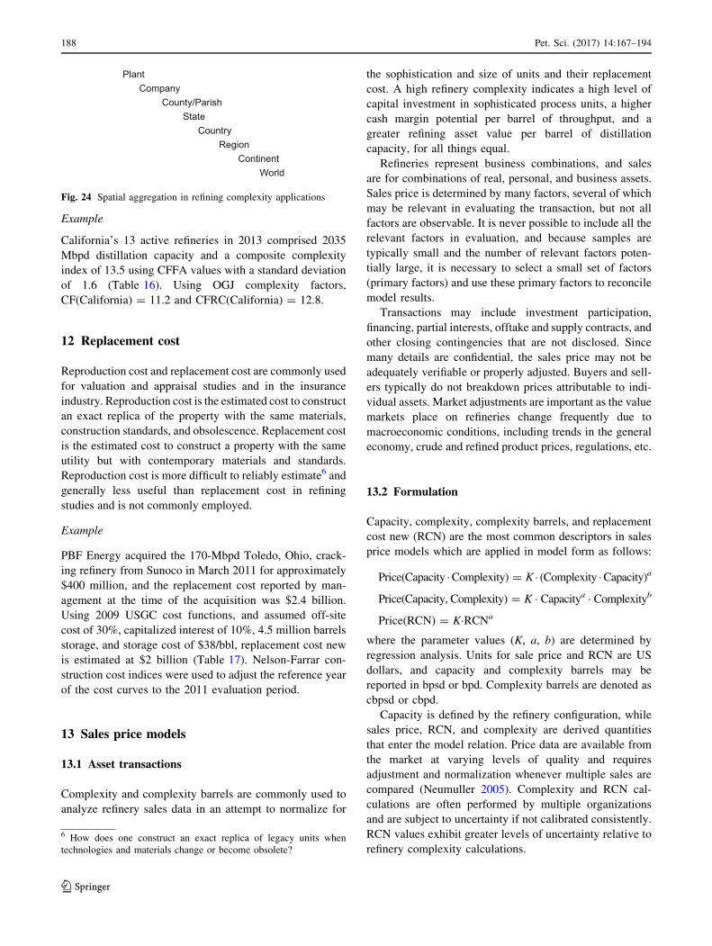
11 Spatial complexity
Refining complexity can be evaluated at any level of spa-
tial aggregation from the plant up through the country level
and beyond (Fig. 24), but as geographic scales expand and
include different states and/or countries, the use of one set
of complexity factors becomes problematic since the data
from which they are derived are typically estimated
regionally. Complexity factors established for the USGC
are not expected to be reliable outside the USA, but
because of the paucity and uncertainty of international
data, it is often used as a proxy. Complexity factors are
computed for a specific region based on regional data, or
adjusted using a location factor (Maples 2000).
Example
Shell Oil Products, USA, operates a 145-MMbpd refinery
in Martinez, California, and a 145-MMbpd refinery in
Anacortes, Washington. Using OGJ 1998 complexity fac-
tors, the complexity index for Shell Oil Products, USA,
combined operations is computed as 12.1 (Table 15).
Using the complexity reference and complexity factor
functional formulations, CFRC(Shell Oil, USA) = 12.2
and CFFA(Shell Oil, USA) = 12.8.
0
5
10
15
20
25
0 20 40 60 80 100
Ref
iner
y co
mpl
exity
Refinery
CF CFRC CFFA
CF
CFRC
CFFA
Fig. 22 Complexity index of US refineries circa 2014 based on OGJ
complexity factors, complexity factor at reference capacity, and
complexity factor functional averages
0
10
20
30
40
<2 2-4 4-6 6-8 8-10 10-12 12-14 14-16 16-18 ≥ 18
Ref
iner
ies
Refinery complexity
CF CFRC CFFA
Fig. 23 Complexity index distribution of US refineries circa 2014
based on OGJ complexity factors, complexity factor at reference
capacities, and complexity factor functional averages
Table 14 PBF Energy’s Delaware City refinery complexity moments (2014)
Capacity, Mbpd Qi/Q0 (Qi/Q0)2 CFFAi SD(CFFAi) E[CI(R)] V(CFFAi)
Atmospheric distillation 190 1.00 1.00 1.0 0.0 1.0 0.0
Vacuum distillation 102 0.54 0.29 1.5 0.7 0.8 0.1
Fluid catalytic cracking 82 0.43 0.19 4.1 1.6 1.8 0.5
Hydrotreating 160 0.84 0.71 2.1 0.9 1.8 0.6
Hydrocracking 18 0.09 0.01 10.9 3.2 1.0 0.1
Catalytic reforming 43 0.23 0.05 4.0 1.6 0.9 0.1
Benzene/toluene extraction 15 0.08 0.01 7.9 7.1 0.6 0.3
Butane isomerization 6 0.03 0.00 6.0 2.3 0.2 0.01
Alkylation 11 0.06 0.00 6.4 2.1 0.4 0.01
Polymerization 16 0.08 0.01 17.5 7.1 1.5 0.4
Fluid coking 47 0.25 0.06 7.5 2.4 1.9 0.4
Hydrogen (MMcfd) 62 0.33 0.11 3.7 3.3 1.2 1.1
Refinery complexity 13.0 3.6
Pet. Sci. (2017) 14:167–194 187
123
Example
California’s 13 active refineries in 2013 comprised 2035
Mbpd distillation capacity and a composite complexity
index of 13.5 using CFFA values with a standard deviation
of 1.6 (Table 16). Using OGJ complexity factors,
CF(California) = 11.2 and CFRC(California) = 12.8.
12 Replacement cost
Reproduction cost and replacement cost are commonly used
for valuation and appraisal studies and in the insurance
industry. Reproduction cost is the estimated cost to construct
an exact replica of the property with the same materials,
construction standards, and obsolescence. Replacement cost
is the estimated cost to construct a property with the same
utility but with contemporary materials and standards.
Reproduction cost is more difficult to reliably estimate6 and
generally less useful than replacement cost in refining
studies and is not commonly employed.
Example
PBF Energy acquired the 170-Mbpd Toledo, Ohio, crack-
ing refinery from Sunoco in March 2011 for approximately
$400 million, and the replacement cost reported by man-
agement at the time of the acquisition was $2.4 billion.
Using 2009 USGC cost functions, and assumed off-site
cost of 30%, capitalized interest of 10%, 4.5 million barrels
storage, and storage cost of $38/bbl, replacement cost new
is estimated at $2 billion (Table 17). Nelson-Farrar con-
struction cost indices were used to adjust the reference year
of the cost curves to the 2011 evaluation period.
13 Sales price models
13.1 Asset transactions
Complexity and complexity barrels are commonly used to
analyze refinery sales data in an attempt to normalize for
the sophistication and size of units and their replacement
cost. A high refinery complexity indicates a high level of
capital investment in sophisticated process units, a higher
cash margin potential per barrel of throughput, and a
greater refining asset value per barrel of distillation
capacity, for all things equal.
Refineries represent business combinations, and sales
are for combinations of real, personal, and business assets.
Sales price is determined by many factors, several of which
may be relevant in evaluating the transaction, but not all
factors are observable. It is never possible to include all the
relevant factors in evaluation, and because samples are
typically small and the number of relevant factors poten-
tially large, it is necessary to select a small set of factors
(primary factors) and use these primary factors to reconcile
model results.
Transactions may include investment participation,
financing, partial interests, offtake and supply contracts, and
other closing contingencies that are not disclosed. Since
many details are confidential, the sales price may not be
adequately verifiable or properly adjusted. Buyers and sell-
ers typically do not breakdown prices attributable to indi-
vidual assets. Market adjustments are important as the value
markets place on refineries change frequently due to
macroeconomic conditions, including trends in the general
economy, crude and refined product prices, regulations, etc.
13.2 Formulation
Capacity, complexity, complexity barrels, and replacement
cost new (RCN) are the most common descriptors in sales
price models which are applied in model form as follows:
Price(Capacity �Complexity) = K � (Complexity �Capacity)a
Price(Capacity, Complexity) = K � Capacitya � Complexityb
Price(RCN) = K�RCNa
where the parameter values (K, a, b) are determined by
regression analysis. Units for sale price and RCN are US
dollars, and capacity and complexity barrels may be
reported in bpsd or bpd. Complexity barrels are denoted as
cbpsd or cbpd.
Capacity is defined by the refinery configuration, while
sales price, RCN, and complexity are derived quantities
that enter the model relation. Price data are available from
the market at varying levels of quality and requires
adjustment and normalization whenever multiple sales are
compared (Neumuller 2005). Complexity and RCN cal-
culations are often performed by multiple organizations
and are subject to uncertainty if not calibrated consistently.
RCN values exhibit greater levels of uncertainty relative to
refinery complexity calculations.
PlantCompany
County/ParishState
CountryRegion
ContinentWorld
Fig. 24 Spatial aggregation in refining complexity applications
6 How does one construct an exact replica of legacy units when
technologies and materials change or become obsolete?
188 Pet. Sci. (2017) 14:167–194
123

Example
A sample7 of refinery transactions between 2010 and 2012
is used to illustrate the computational methods and models
(Table 18). The transaction data includes whether the
refinery was active at the time of sale, and the sales data
excludes pipelines, terminals, and inventory. Replacement
costs new were estimated by the purchaser and were not
reported for all sales.
The weighted average sales price per barrel for the sample
is $1665/bpd, and the weighted average sales price per com-
plexity barrel is $152/cbpd (Table 19). Standard deviations
are the same order as the averages $1591/bpd and $202/cbpd,
respectively, indicating wide variation in market valuations.
Idle (mothballed) refineries at the timeof sale sell at a discount
relative to active refineries. The average sales price for active
refineries is $2723/bpd, and the average sales price per com-
plexity barrel is $238/cbpd; for inactive refineries, the average
sales prices are $1067/bpd and $114/cbpd.
The average replacement cost per capacity barrel is
$16,600/bpd with $9800/bpd standard deviation. Sales
price per replacement cost averaged 12% with a 4.5%
standard deviation. Refinery assets are normally purchased
at a discount to replacement cost, and then, capital is spent
to upgrade and improve the plant equipment and product
slate and crude supply access. The price discount for this
Table 15 Shell Oil Products,
USA, corporate complexity
(2014)
Capacity, Mbpd ADU capacity, % CF CI
Atmospheric distillation 290 100 1 1.0
Vacuum distillation 157 54 2 1.1
Coking 70 24 6 1.4
Catalytic cracking 121 42 6 2.5
Catalytic reforming 62 22 5 1.1
Hydrocracking 37 13 6 0.8
Hydrotreating 249 86 2 1.7
Alkylation 23 8 10 0.8
Isomerization 22 8 15 1.1
Polymerization 6.8 2 10 0.2
Hydrogen (MMcfd) 108 37 1 0.4
Shell Oil Products complexity 12.1
Shell Oil Products, USA, refineries include a 145-Mbpd refinery in Martinez, California, and a 145-Mbpd
refinery in Anacortes, Washington
Table 16 California state
refining complexity (2013)Capacity, Mbpd ADU capacity, % CFFA CI
Atmospheric distillation 2035 100 1.0 1.0
Vacuum distillation 1162 57 1.5 0.8
Delayed coking 458 23 7.5 1.7
Thermal operations 10 0.5 2.8 0.0
Catalytic cracking 660 32 4.1 1.3
Catalytic reforming 416 20 4.0 0.8
Catalytic hydrocracking 484 24 10.9 2.6
Catalytic hydrotreating 1698 83 2.1 1.8
Alkylation 176 9 6.4 0.5
Polymerization 9 0.4 17.5 0.1
Aromatics – – 7.9 –
Isomerization 155 8 6.0 0.5
Lubes 20 1 9.0 0.1
Oxygenates – – 1.6 –
Hydrogen (MMcfd) 1229 60 3.7 2.3
Asphalt 62 3 1.5 0.05
California complexity (SD) 13.5(1.6)
Standard deviation for complexity factor functional specification denoted in parenthesis
7 The results are not intended to be representative of the broader
market.
Pet. Sci. (2017) 14:167–194 189
123

Table 17 PBF Energy’s
Toledo, Ohio, refinery
replacement cost estimate
(2013)
Capacity,
Mbpd
C = KQa 2009 cost,
$million
2011 cost,
$millionK a
Atmospheric distillation 170 8.20 0.51 113 143
Fluid catalytic cracking 79 24.67 0.46 185 235
Gasoline hydtrotreating 95 4.96 0.58 70 88
Catalytic hydrocracking 45 21.45 0.72 329 417
Catalytic reforming 45 12.19 0.55 98 124
Alkylation 10 12.19 0.61 49 62
Polymerization 7.0 18.65 0.60 60 76
BTX 16 12.48 0.61 69 88
Tank farm with storage 4500 171
Total on-sites 1405
Off-site (30%) 421
Total facility cost 1826
Capitalized interest (10%) 183
Replacement cost 2009
Cost functions based on Kaiser and Gary (2009)
Table 18 Select US and one international refinery transaction (2010–2012). Source: Company 10-K, industry press
Buyer Seller Year Location Capacity,
Mbpd
CI Active at
sale
Sales price,
$million
RCN,
$million
Alon Flying J 2010 Bakersfield, CA 68 8.8 ? 40
PBF Valero 2010 Paulsboro, NJ 168 13.2 ? 358 5800
PBF Valero 2010 Delaware City, DE 190 11.3 – 220
PBF Sunoco 2011 Toledo, OH 170 9.2 ? 400 2400
Valero Chevron 2011 Pembroke, Wales 220 11.8 ? 480 3400
Valero Murphy 2011 Meraux, LA 135 10.2 ? 325
Calumet Murphy 2011 Superior, WI 35 8.1 ? 214
Tesoro BP 2012 Carson City, CA 266 13.3 ? 175 1167
Delta Phillips 66 2012 Trainer, PA 185 7.4 – 180 2700
Table 19 Sales metrics for
select refinery transactions
(2010–2012)
Refinery PriceBarrel
,
$/bpd
PriceCBarrel
,
$1000/cbpd
PriceRCN
,
%
RCNBarrel
,
$1000/bpd
Bakersfield, CA 588 67
Toledo, OH 2353 256 17 14.1
Paulsboro, NJ 2131 161 6.2 34.5
Delaware City, DE 1158 102
Pembroke, Wales 2182 185 14 15.5
Meraux, LA 2407 236
Superior, WI 6114 755
Carson City, CA 658 49 15 4.4
Trainer, PA 973 131 6.7 14.6
Average 1665 152 12 16.6
190 Pet. Sci. (2017) 14:167–194
123

sample and time period is relatively steep; earlier in the
decade discounts typically averaged between 25 to 40%.
Using the refinery sales for active units, the parameters
of the sales price models are estimated as follows:
Price = 0.80 (Complexity � Capacity)1.39, R2 = 0.85
Price = 0.11 Capacity1.69 Complexity0.66, R2 = 0.87
Price = 14.7 RCN0.39, R2 = 0.39
13.3 Constraints
Using transactions is a strong indicator of value because it
reflects the actions of buyers and sellers in the market.
Multifactor regression models are limited in their ability to
capture all of the relevant factors of transactions, however,
because sample sizes are usually much smaller than the
factor set, and so a small number of factors are usually
selected for evaluation. The critical ingredient is to select
‘‘comparable’’ sales and to perform ‘‘suitable’’ adjustments
prior to parameter estimation, but these activities are sub-
ject to user preferences and experience. Two transactions
are never the same. Standard practice usually requires the
consideration of actual sales data, if available, in appraising
a property. Complexity and complexity barrels find com-
mon use in reporting market data and transaction metrics.
14 Complexity barrels
Fitch, Moody’s, Standards & Poor (S&P) and other rating
agencies use complexity barrels, also referred to as
equivalent distillation capacity, in their assessment of the
credit rating of companies (Fitch 2012; Moody’s 2013;
S&P 2011). As the name implies, complexity barrels are
simply the product of distillation capacity and refinery
complexity and, because it incorporates both the size of the
refinery and its overall complexity, are considered a useful
measure for comparison and trending purposes. Complex-
ity barrels recognize a company’s throughput capacity and
signal the quality of that capacity via the refining
complexity.
Example
The equivalent distillation capacity of Exxon Mobil’s
Baton Rouge refinery increased by 170 cbpd, or about 4%,
from 2000 to 2013. Exxon Mobil’s Baton Rouge refinery
configuration and complexity has not changed significantly
over the past decade, and therefore, its complexity barrels
have also not changed significantly (Table 20).
The purpose of rating agencies is to assess the likeli-
hood a company will repay its debt, the interest, and
principal on its bonds. Agencies use a letter and number
system to rate corporate bonds, and the lower the bond
rating, the higher the interest required on the bond issue
since ratings correlate with the probability of corporate
default (Table 21). High bond ratings are associated with
lower interest rates and lower risk of default than low
bond ratings. Each rating agency applies different
Table 20 Exxon Mobil’s Baton Rouge refinery data (2000–2013)
Year ADU capacity,
Mbpd
CI Complex barrels,
Mcbpd
2000 485 9.5 4592
2001 489 9.6 4664
2002 489 9.6 4705
2003 492 9.7 4757
2004 494 10.3 5088
2005 494 10.3 5090
2006 501 10.2 5110
2007 503 10.2 5121
2008 503 10.2 5116
2009 503 10.2 5128
2010 505 10.2 5152
2011 504 9.9 4985
2012 503 10.5 5292
2013 503 9.5 4762
Table 21 Moody’s corporate
bond rating system and historic
default rates. Source: Moody’s
(2013)
Rating Description Default rate, %
One year Five years
Aaa Highest quality, referred to as ‘‘gilt edge’’ 0.00 0.09
Aa High quality, known as ‘‘high-grade bonds’’ 0.02 0.32
A Upper medium-grade 0.06 0.78
Baa Currently safe, but could be subject to impairment 0.16 1.5
Ba Speculative bond 1.0 7.6
B Chance of bonds being paid off is small 3.4 17.9
Caa Poor quality and may already be in default 11.8 35.5
Ca/C Highly speculative/lowest quality and poor prospects 37.2 52.7
Pet. Sci. (2017) 14:167–194 191
123

methodologies, thresholds and notation, but they are
broadly similar across the industry.
Rating agencies use a weighted risk index based on
several financial and operational components of the com-
pany, including refinery configuration, capital leverage,
competition, and other factors. Equivalent distillation
capacity is one component of ratings that is taken into
account, and the greater the value the higher the rating.
Complexity barrels, Mcbpd Rating
C9000 Aaa
7500–9000 Aa
5000–7500 A
3500–5000 Baa
2000–3500 Ba
500–2000 B
\500 Caa
Source: Moody’s (2013).
Example
In 2014, Western Refining owned a 122-Mbpd refinery
with a complexity index of 5.2, and a 26-Mbpd refinery
with a complexity index of 9.6. Western Refining’s com-
plexity barrels are computed as (122 Mbpd) (5.2) ? (26
Mbpd) (9.6) = 884 Mcbpd, which would be assigned a B
component rating using Moody’s system. The product of
the corporate complexity index and total capacity is usually
a good proxy if individual plant data are unavailable.
Western Refining’s 5.9 corporate complexity index yields
an equivalent distillation capacity of 873 Mcbpd.
15 Inverse problem
Complexity factors are the key ingredient in computing
refinery complexity and are often sold as part of a com-
mercial database, which explains why they are often
viewed as proprietary. This perspective is misguided,
however, and there is no reason to think of complexity
factors as confidential since they can always be inferred by
solving a system of linear equations using the refinery
complexity relations.
If Q = (Q0, Q1, …, Qn) and CF = (1, CF1, CF2, …,
CFn) are given, the complexity index of refinery R is
computed as the inner product of the vectors divided by
Q0, or CI(R) = Q � CFT/Q0. In the inverse problem, the
complexity factors are unknown, and the task is to infer
their value based on (reported) refinery complexity.
Refinery complexities are frequently reported in company
financial statements and press releases, among other
sources. If there are n complexity factors to infer, there
needs to be n refinery indices available for plants with
roughly similar process units. A three refinery example
illustrates the procedure followed by the general
framework.
15.1 Three refinery example
Three international refineries located in the same country and
containing vacuumdistillation, reforming, and hydrotreating
capacity report complexity indices CI(A) = 3.9,
CI(B) = 4.0, and CI(C) = 5.5 in investor presentations but
do not disclose the complexity factors used in the calculation.
Refinery configurations are as follows:
A, Mbpd B, Mbpd C, Mbpd
Atmospheric distillation 100 80 50
Vacuum distillation 40 45 30
Catalytic reforming 20 15 10
Hydrotreating 30 20 35
Since there are three refining units besides atmospheric
distillation, three equations are needed to estimate the three
complexity factors. First, write the complexity equation for
each refinery:
CIðAÞ ¼ 100 Mbpd
100 MbpdCFADU þ 40 Mbpd
100 MbpdCFVDU þ 20 Mbpd
100 MbpdCFCCR þ 30 Mbpd
100 MbpdCFHT
CIðBÞ ¼ 80 Mbpd
80 MbpdCFADU þ 45 Mbpd
80 MbpdCFVDU þ 15 Mbpd
80 MbpdCFCCR þ 20 Mbpd
80 MbpdCFHT
CIðCÞ ¼ 50 Mbpd
50 MbpdCFADU þ 30 Mbpd
50 MbpdCFVDU þ 10 Mbpd
50 MbpdCFCCR þ 35 Mbpd
50 MbpdCFHT
8>>>>>>><
>>>>>>>:
192 Pet. Sci. (2017) 14:167–194
123

Next, assume CFADU = 1, and solve for the unknowns:
3:9 ¼ ð1Þð1Þ þ 0:4CFVDU þ 0:2CFCCR þ 0:3CFHT
4:0 ¼ ð1Þð1Þ þ 0:56CFVDU þ 0:19CFCCR þ 0:25CFHT
5:5 ¼ ð1Þð1Þ þ 0:6CFVDU þ 0:2CFCCR þ 0:7CFHT
8><
>:
Solving the system of equations yields CFVDU = 2,
CFCCR = 6, and CFHT = 3, the (inferred) complexity
factors used in the evaluation.
15.2 Matrix formulation
Let (Qi0;Q
i1; . . .;Q
inÞ denote the process capacities and
CI(Ri) the complexity index of refinery Ri, i = 1, 2, …,
n. Denote the complexity indices of the n refineries in
vector form as CI = (CI(R1), CI(R2), …, CI(Rn)) and the
complexity factors of the process units as CF = (1, CF1 …,
CFn). The refining equations for the n refineries are
expressed as a matrix, which is readily verified to yield the
refinery equations:
CIðR1ÞCIðR2Þ
..
.
CIðRnÞ
0
BBB@
1
CCCA ¼
1 Q11=Q
10 � � � Q1
n=Q10
1 Q21=Q
20 � � � Q2
n=Q20
..
. ...
� � � ...
1 Qn1=Q
n0 � � � Qn
n=Qn0
0
BBB@
1
CCCA
1
CF1
..
.
CFn
0
BBB@
1
CCCA
or, in matrix form:
CIT = ~M � CFT,
To solve for the complexity factors, invert the matrix
and solve the system of equations. As long as the equations
are well conditioned, which they almost always will be
because of the unique nature of refinery configurations—
literally, no two refineries are alike in process capacities—
the complexity factors are computed thus:
CFT = ~M�1 � CI
Example
Five international refineries located in the same country
report complexity indices CI(A) = 7.1, CI(B) = 6.7,
CI(C) = 6.8, CI(D) = 7.6, and CI(E) = 5.7 in their annual
reports. Refinery configurations are as follows:
A,
Mbpd
B,
Mbpd
C,
Mbpd
D,
Mbpd
E,
Mbpd
Atm. distillation 120 100 80 155 60
Vacuum
distillation
60 40 35 70 25
Thermal
operation
30 20 30 40 10
Cat.
hydrocracking
30 25 15 40 10
Reforming 15 10 12 30 8
Hydrotreating 50 45 30 70 20
Refinery
complexity
7.1 6.7 6.8 7.6 5.7
Set up the refinery equation for the unknown variables
and solve.
CIðAÞCIðBÞCIðCÞCIðDÞCIðEÞ
0BBBBBB@
1CCCCCCA
¼
1 60=120 30=120 30=120 15=120 50=1201 40=100 20=100 25=100 10=100 45=1001 35=80 30=80 15=80 12=80 30=801 70=155 40=155 40=155 30=155 70=1551 25=60 10=60 10=60 8=60 20=60
0BBBB@
1CCCCA
1
CFVDUCFTOCFHCCFCCRCFHT
0BBBBBB@
1CCCCCCA
7:1 ¼ ð1Þð1Þ þ 0:5CFVDU þ 0:25CFTO þ 0:25CFHC þ 0:13CFCCR þ 0:42CFHT
6:7 ¼ ð1Þð1Þ þ 0:4CFVDU þ 0:2CFTO þ 0:25CFHC þ 0:1CFCCR þ 0:45CFHT
6:8 ¼ ð1Þð1Þ þ 0:44CFVDU þ 0:38CFTO þ 0:19CFHC þ 0:15CFCCR þ 0:38CFHT
7:6 ¼ ð1Þð1Þ þ 0:45CFVDU þ 0:26CFTO þ 0:26CFHC þ 0:19CFCCR þ 0:45CFHT
5:7 ¼ ð1Þð1Þ þ 0:42CFVDU þ 0:17CFTO þ 0:3CFHC þ 0:13CFCCR þ 0:33CFHT
8>>>>>><
>>>>>>:
Pet. Sci. (2017) 14:167–194 193
123
Using Excel’s Solver function yields CFVDU = 2,
CFTO = 3, CFHC = 9, CFCCR = 6.5, and CFHT = 3.
Open Access This article is distributed under the terms of the
Creative Commons Attribution 4.0 International License (http://crea
tivecommons.org/licenses/by/4.0/), which permits unrestricted use,
distribution, and reproduction in any medium, provided you give
appropriate credit to the original author(s) and the source, provide a
link to the Creative Commons license, and indicate if changes were
made.
References
BP p.l.c. 2015. BP statistical review of world energy June 2015.
http://www.bp.com/content/dam/bp/pdf/Energy-economics/statis
tical-review-2015/bp-statistical-review-of-world-energy-2015-
full-report.pdf. Accessed 17 Sept 2015.
Farrar GL. How Nelson cost indices are compiled. OGJ.
1985;(65):145.
Farrar GL. Interest reviving in complexity factors. OGJ. 1989;(69):90.
Fitch Ratings Inc. Special report—rating oil refining and marketing
companies. 2012.
Gary JH, Handwerk GE, Kaiser MJ. Petroleum refining: technology
and economics. 5th ed. Boca Raton: CRC Press; 2007. doi:10.
1016/B0-12-227410-5/00556-1.
Kaiser MJ. A new approach to refinery complexity factors. Engi-
neering Economist. 2016;30(4):1–33. doi:10.1080/0013791X.
2016.1202365.
Kaiser MJ, Gary JH. Refinery cost functions in the U.S. Gulf Coast.
Pet Sci Technol. 2009;27(2):168–81. doi:10.1080/
10916460701434704.
Maples RE. Petroleum refining process economics. 2nd ed. Tulsa,
OK: PennWell; 2000.
Meyers RA. Handbook of petroleum refining processes. 3rd ed. New
York: McGraw-Hill; 2004.
Moody’s Investors Service. Global refining and marketing rating
methodology. 2013.
Nelson WL. Guild to refinery operating cost (process costimating).
3rd ed. Tulsa, OK: Petroleum Publishing; 1976a.
Nelson WL. How the Nelson refinery construction-cost indexes
evolved. OGJ. 1976b;(56):68.
Nelson WL. Here’s how operating cost indexes are computed. OGJ.
1977;(57):86.
Neumuller R. Method estimates U.S. refinery fixed costs. OGJ.
2005;(85):43.
Oil and Gas Journal. 2014. Worldwide refining survey. Tulsa, OK:
PennWell. 2015. http://www.ogj.com/ogj-survey-downloads.
html. Accessed 17 Sept 2015.
Parkash S. Refining process handbook. Amsterdam: Elsevier; 2003.
Raseev S. Thermal and catalytic processes in petroleum refining. New
York: Marcel Dekker; 2003. doi:10.1201/9780203912300.
Riazi MR, Eser S, Agrawal SS, Diez JL Pena (Ed). Petroleum refining
and natural gas processing. MNL58, ASTM international, West
Conchohocken; 2013. doi:10.1520/MNL58-EB.
Schobert HJ. Energy and society. New York: Taylor and Francis;
2002.
Speight JG. The chemistry and technology of petroleum. 3rd ed. New
York: Marcel Dekker Inc; 1998. doi:10.1201/9780824742119.
Standard & Poor’s Financial Services LLC. Key credit factors:
criteria for rating the global oil refining industry; 2011.
U.S. Department of Energy, Energy Information Administration
(EIA). U.S. exports of petroleum products. 2015a. http://www.
eia.gov/dnav/pet/pet_move_exp_dc_NUS-Z00_mbbl_m.htm.
Accessed 17 Sept 2015.
U.S. Department of Energy, Energy Information Administration
(EIA). U.S. field production of crude oil. 2015b. http://www.eia.
gov/dnav/pet/hist/LeafHandler.ashx?n=PET&s=
MCRFPUS1&f=M. Accessed 17 Sept 2015.
U.S. Department of Energy, Energy Information Administration
(EIA). U.S. imports of crude oil. 2015c. http://www.eia.gov/
dnav/pet/hist/LeafHandler.ashx?n=pet&s=mcrimus1&f=a.
Accessed 17 Sept 2015.
U.S. Department of Energy, Energy Information Administration
(EIA). U.S. refinery net product. 2015d. http://www.eia.gov/
dnav/pet/pet_pnp_refp2_dc_nus_mbbl_m.htm. Accessed 17 Sept
2015.
U.S. Department of Labor, Occupational Safety and Health Admin-
istration (OSHA), OSHA technical manual, in PetroleumRefining Processes, Washington, D.C., 2005, sec. IV, chap. 2.
194 Pet. Sci. (2017) 14:167–194
123


