
A Revisit to Quadratic Programming with One Inequality
Quadratic Constraint via Matrix Pencil ∗
Yong Hsia∗ Gang-Xuan Lin† Ruey-Lin Sheu†
December 3, 2013
Abstract
The quadratic programming over one inequality quadratic constraint (QP1QC) is a very
special case of quadratically constrained quadratic programming (QCQP) and attracted much
attention since early 1990’s. It is now understood that, under the primal Slater condition,
(QP1QC) has a tight SDP relaxation (PSDP). The optimal solution to (QP1QC), if exists, can
be obtained by a matrix rank one decomposition of the optimal matrix X∗ to (PSDP). In this
paper, we pay a revisit to (QP1QC) by analyzing the associated matrix pencil of two symmetric
real matrices A and B, the former matrix of which defines the quadratic term of the objective
function whereas the latter for the constraint. We focus on the “undesired” (QP1QC) problems
which are often ignored in typical literature: either there exists no Slater point, or (QP1QC) is
unbounded below, or (QP1QC) is bounded below but unattainable. Our analysis is conducted
with the help of the matrix pencil, not only for checking whether the undesired cases do happen,
but also for an alternative way otherwise to compute the optimal solution in comparison with
the usual SDP/rank-one-decomposition procedure.
Keywords: Quadratically constrained quadratic program, matrix pencil, hidden convexity,
Slater condition, unattainable SDP, simultaneously diagonalizable with congruence.
1 Introduction
Quadratically constrained quadratic programming (QCQP) is a classical nonlinear optimization
problem which minimizes a quadratic function subject to a finite number of quadratic constraints.
∗This research was supported by Taiwan National Science Council under grant 102-2115-M-006-010, by National
Center for Theoretical Sciences (South), by National Natural Science Foundation of China under Grants 11001006
and 91130019/A011702, and by the fund of State Key Laboratory of Software Development Environment under grant
SKLSDE-2013ZX-13.∗LMIB of the Ministry of Education; School of Mathematics and System Sciences, Beihang University, Beijing,
100191, P. R. China ([email protected]).†Department of Mathematics, National Cheng Kung University, Taiwan ([email protected]).
1

2
A general (QCQP) problem can not be solved exactly and is known to be NP-hard. The (QCQP)
problems with a single quadratic inequality constraint, however, are polynomially solvable. It carries
the following format
(QP1QC) : inf F (x) = xTAx− 2fTx
s.t. G(x) = xTBx− 2gTx ≤ µ,(1)
where A,B are two n×n real symmetric matrices, µ is a real number and f, g are two n×1 vectors.
The problem (QP1QC) arises from many optimization algorithms, most importantly, from the
trust region methods. See, e.g., [9, 16] in which B � 0 and g = 0. Extensions to an indefinite B
but still with g = 0 are considered in [2, 8, 14, 20, 24]. Direct applications of (QP1QC) having a
nonhomogeneous quadratic constraint can be found in solving an inverse problem via regularization
[6, 10] and in minimizing the double well potential function [5]. Solution methods for the general
(QP1QC) can be found in [7, 15, 18].
As we can see from the above short list of review, it was not immediately clear until rather
recent that the problem (QP1QC) indeed belongs to the class P. Two types of approaches have been
most popularly adopted: the (primal) semidefinite programming (SDP) relaxation and the Lagrange
dual method. Both require the (QP1QC) problem to satisfy either the primal Slater condition (e.g.,
[7, 15, 24, 25]):
Primal Slater Condition: There exists an x0 such that G(x0) = xT0 Bx0 − 2gTx0 < µ;
and/or the dual Slater condition (e.g., [2, 7, 15, 24, 25]):
Dual Slater Condition: There exists a σ′ ≥ 0 such that A+ σ′B � 0.
Nowadays, with all the efforts and results in the literature, (QP1QC) is no longer a difficult problem
and its structure can be comprehended easily by means of a standard SDP method, the conic duality,
the S-lemma, and a rank-one decomposition procedure.
Under the primal Slater condition, the Lagrangian function of (QP1QC) is
d(σ) = infx∈Rn
L(x, σ) := xT (A+ σB)x− 2(f + σg)Tx− µσ, σ ≥ 0, (2)
with which the dual problem of (QP1QC) can be formulated as
(D) supσ≥0
d(σ).
Using Shor’s relaxation scheme [19], the above Lagrange dual problem (D) has a semidefinite pro-
gramming reformulation:
(DSDP) : sup s
s.t.
[A+ σB −f − σg−fT − σgT −µσ − s
]� 0,
σ ≥ 0.
(3)

3
The conic dual of (DSDP) turns out to be the SDP relaxation of (QP1QC):
(PSDP) : inf
[A −f−fT 0
]• Y
s.t.
[B −g−gT −µ
]• Y ≤ 0,
Yn+1,n+1 = 1
Y � 0,
(4)
where X • Y := trace(XTY ) is the usual matrix inner product. Let v(·) denote the optimal value of
problem (·). By the weak duality, we have
v(QP1QC) ≥ v(PSDP) ≥ v(DSDP). (5)
To obtain the strong duality, observe that
v(QP1QC) = infx∈R
{F (x)
∣∣∣∣G(x) ≤ µ}
= sup
{s ∈ R
∣∣∣∣ {x ∈ Rn|F (x)− s < 0, G(x)− µ ≤ 0} = ∅}.
Under the primal Slater condition and by the S-lemma [18], we get
sup
{s ∈ R
∣∣∣∣ {x ∈ Rn|F (x)− s < 0, G(x)− µ ≤ 0} = ∅}
= sup
{s ∈ R
∣∣∣∣∃σ ≥ 0 such that F (x)− s+ σG(x)− σµ ≥ 0, ∀x ∈ Rn}
=
sup s
s.t.
[A+ σB −f − σg−fT − σgT −µσ − s
]•
[xxT x
xT 1
]≥ 0, ∀x ∈ Rn
σ ≥ 0
=
sup s
s.t.
[A+ σB −f − σg−fT − σgT −µσ − s
]� 0
σ ≥ 0,
(6)
where the last equality holds because[A+ σB −f − σg−fT − σgT −µσ − s
]•[
xxT x
xT 1
]≥ 0, ∀x ∈ Rn ⇔
[A+ σB −f − σg−fT − σgT −µσ − s
]� 0.
Combining (3), (5) and (6) together, we conclude that
v(QP1QC) = v(PSDP) = v(DSDP), (7)
which says that the SDP relaxation of (QP1QC) is tight. The strong duality result also appeared,
e.g., in [4, Appendix B].

4
To obtain a rank-one optimal solution of (PSDP) having the format X∗ =[(x∗)
T, 1]T [
(x∗)T, 1],
Sturm and Zhang [21] provides the following rank-one decomposition procedure. Suppose X∗ is a
positive semidefinite optimal matrix obtained from solving (PSDP) and the rank of X∗ is r. First
compute a rank one decomposition X∗ =∑ri=1 pip
Ti . Denote
M(G) =
[B −g−gT −µ
].
If(pT1 M(G)p1
) (pTi M(G)pi
)≥ 0 for all i = 1, 2, . . . , r, set y = p1. Otherwise, set y =
p1 + αpj√1 + α2
where(pT1 M(G)p1
) (pTj M(G)pj
)< 0 and α satisfies (p1 + αpj)
TM(g) (p1 + αpj) = 0. Then, X∗ =
X∗−yyT is an optimal solution for (PSDP) of rank r−1. Repeat the procedure until X∗ is eventually
reduced to a rank one matrix.
Clearly, by the SDP relaxation, first one lifts the (QP1QC) problem into a linear matrix inequality
in a (much) higher dimensional space where a conic (convex) optimization problem (PSDP) is solved,
then followed by a matrix rank-one decomposition procedure to run it back to a solution of (QP1QC).
The idea is neat, but it suffers from a huge computational task should a large scale (QP1QC) be
encountered.
In contrast, the Lagrange dual approach seems to be more natural but the analysis is often sub-
ject to serious assumptions. We can see that the Lagrange function (2) makes a valid lower bound
for the (QP1QC) problem only when A+ σB � 0. Furthermore, the early analysis, such as those in
[2, 7, 15, 24, 25], all assumed the dual Slater condition in order to secure the strong duality result.
Actually, the dual Slater condition is a very restrictive assumption since it implies that, see [13], the
two matrices A and B can be simultaneously diagonalizable via congruence (SDC), which itself is
already very limited:
Simultaneously Diagonalizable via Congruence (SDC): A and B are simultaneously diago-
nalizable via congruence (SDC) if there exists a nonsingular matrix C such that both CTAC and
CTBC are diagonal.
Nevertheless, solving (QP1QC) via the Lagrange dual enjoys a computational advantage over
the SDP relaxation. It has been studied thoroughly in [7] that the optimal solution x∗ to (QP1QC)
problems, while satisfying the dual Slater condition, is either x = limσ→σ∗
(A + σB)−1(f + σg), or
obtained from x + α0x where σ∗ is the dual optimal solution, x is a vector in the null space of
A+ σ∗B and α0 is some constant from solving a quadratic equation. For (QP1QC) problems under
the SDC condition while violating the dual Slater condition, they are either unbounded below or
can be transformed equivalently to an unconstraint quadratic problem. Since the dual problem is
a single-variable concave programming, it is obvious that the computational cost for x∗ using the
dual method is much cheaper than solving a semidefinite programming plus an additional run-down
procedure.

5
Our paper pays a revisit to (QP1QC) trying to solve it by continuing and extending the study
beyond the dual Slater condition A + σB � 0 (or SDC) into the hard case that A + σB � 0. Our
analysis was motivated by an early result by J. J. More [15, Theorem 3.4] in 1993, which states:
Under the primal Slater condition and assuming that B 6= 0, a vector x∗ is a global minimizer
of (QP1QC) if and only if there exists a pair (x∗, σ∗) ∈ Rn × R such that x∗ is primal feasible
satisfying x∗TBx∗ − 2gTx∗ ≤ µ; σ∗ ≥ 0 is dual feasible; the pair satisfies the complementarity
σ∗(x∗TBx∗ − 2gTx∗ − µ) = 0; and a second order condition A+ σ∗B � 0 holds.
Notice that the speciality of the statement is to obtain a strengthening version of the second order
necessary condition A+σ∗B � 0. Normally in the context of a general nonlinear programming, one
can only conclude that A+ σ∗B is positive semidefinite on the tangent subspace of G(x∗) = 0 when
x∗ lies on the boundary. The original proof was lengthy, but it can now be derived from the theory
of semidefinite programming without much difficulty.
In this paper, we first solve (QP1QC) separately without the primal Slater condition in Section
2. In Section 3, we establish new results for the positive semideifinite matrix pencil
I�(A,B) = {σ ∈ R | A+ σB � 0}
with which, in Section 4, we characterize necessary and sufficient conditions for two unsolvable
(QP1QC) cases: either (QP1QC) is unbounded below, or bounded below but unattainable. The
conditions are not only polynomially checkable, but provide a solution procedure to obtain an optimal
solution x∗ of (QP1QC) when the problem is solvable. In Section 5, we use numerical examples to
show why (QP1QC), while failing the (SDC) condition, become the hard case. Conclusion remarks
are made in section 6.
2 (QP1QC) Violating Primal Slater Condition
In this section, we show that (QP1QC) with no Slater point can be separately solved without any
condition. Notice that, if µ > 0, x = 0 satisfies the Slater condition. Consequently, if the primal
Slater condition is violated, we must have µ ≤ 0, and
minx∈Rn
G(x) = xTBx− 2gTx ≥ µ, (8)
which implies that G(x) is bounded from below and thus
B � 0; g ∈ R(B); G(B+g) = −gTB+g ≥ µ
where R(B) is the range space of B, and B+ is the Moore-Penrose generalized inverse of B.
Conversely, if B � 0, then G(x) is convex. Moreover, if g ∈ R(B), the set of critical points
6
{x∣∣Bx = g
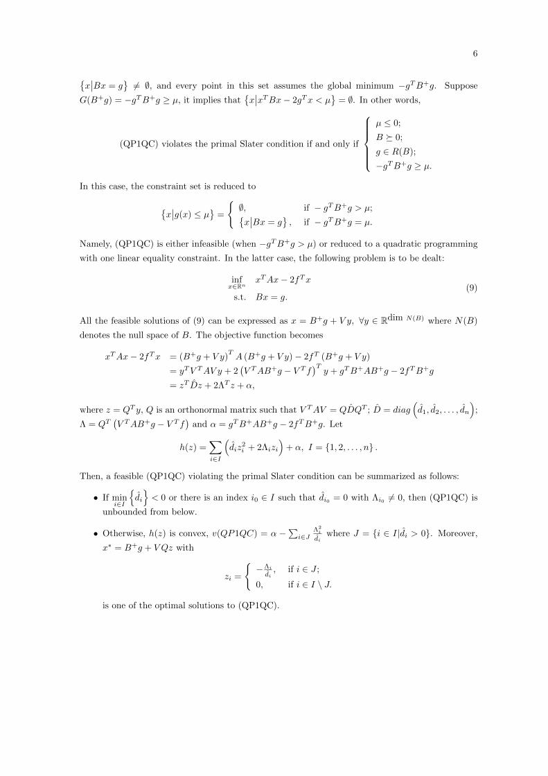
}6= ∅, and every point in this set assumes the global minimum −gTB+g. Suppose
G(B+g) = −gTB+g ≥ µ, it implies that{x∣∣xTBx− 2gTx < µ
}= ∅. In other words,
(QP1QC) violates the primal Slater condition if and only if
µ ≤ 0;
B � 0;
g ∈ R(B);
−gTB+g ≥ µ.
In this case, the constraint set is reduced to
{x∣∣g(x) ≤ µ
}=
{∅, if − gTB+g > µ;{x∣∣Bx = g
}, if − gTB+g = µ.
Namely, (QP1QC) is either infeasible (when −gTB+g > µ) or reduced to a quadratic programming
with one linear equality constraint. In the latter case, the following problem is to be dealt:
infx∈Rn
xTAx− 2fTx
s.t. Bx = g.(9)
All the feasible solutions of (9) can be expressed as x = B+g + V y, ∀y ∈ Rdim N(B) where N(B)
denotes the null space of B. The objective function becomes
xTAx− 2fTx = (B+g + V y)TA (B+g + V y)− 2fT (B+g + V y)
= yTV TAV y + 2(V TAB+g − V T f
)Ty + gTB+AB+g − 2fTB+g
= zT Dz + 2ΛT z + α,
where z = QT y, Q is an orthonormal matrix such that V TAV = QDQT ; D = diag(d1, d2, . . . , dn
);
Λ = QT(V TAB+g − V T f
)and α = gTB+AB+g − 2fTB+g. Let
h(z) =∑i∈I
(diz
2i + 2Λizi
)+ α, I = {1, 2, . . . , n} .
Then, a feasible (QP1QC) violating the primal Slater condition can be summarized as follows:
• If mini∈I
{di
}< 0 or there is an index i0 ∈ I such that di0 = 0 with Λi0 6= 0, then (QP1QC) is
unbounded from below.
• Otherwise, h(z) is convex, v(QP1QC) = α −∑i∈J
Λ2i
diwhere J = {i ∈ I|di > 0}. Moreover,
x∗ = B+g + V Qz with
zi =
{−Λi
di, if i ∈ J ;
0, if i ∈ I \ J.
is one of the optimal solutions to (QP1QC).

7
3 New Results on Matrix Pencil and SDC
As we have mentioned before, we will use matrix pencils, that is, one-parameter families of matrices
of the form A + σB as a main tool to study (QP1QC). An excellent survey for matrix pencils can
be found in [22]. In this section, we first summarize important results about matrix pencils followed
by new findings of the paper.
For any symmetric matrices A,B, define
I�(A,B) := {σ ∈ R | A+ σB � 0}, (10)
I�(A,B) := {σ ∈ R | A+ σB � 0}, (11)
II�(A,B) := {(µ, σ) ∈ R2 | µA+ σB � 0}, (12)
II�(A,B) := {(µ, σ) ∈ R2 | µA+ σB � 0}, (13)
Q(A) := {v | vTAv = 0}, (14)
N(A) := {v | Av = 0}. (15)
The first result characterizes when I�(A,B) 6= ∅ and when II�(A,B) 6= ∅.
Theorem 1 ([22]) If A,B ∈ Rn×n are symmetric matrices, then I�(A,B) 6= ∅ if and only if
wTAw > 0, ∀w ∈ Q(B), w 6= 0. (16)
Furthermore, II�(A,B) 6= ∅ implies that
Q(A) ∩Q(B) = {0}, (17)
which is also sufficient if n ≥ 3.
The second result below extends the discussion in Theorem 1 to the positive semidefinite case
I�(A,B) 6= ∅ assuming that B is indefinite. This result was also used by More to solve (QP1QC)
in [15]. An example shown in [15] indicates that the assumption about the indefiniteness of B is
critical.
Theorem 2 ([15]) If A,B ∈ Rn×n are symmetric matrices and B is indefinite, then I�(A,B) 6= ∅if and only if
wTAw ≥ 0, ∀w ∈ Q(B). (18)
Other known miscellaneous results related to our discussion for (QP1QC) are also mentioned
below. In particular, the proof of Lemma 2 is constructive.
Lemma 1 [15] Both I�(A,B) and I�(A,B) are intervals.

8
Lemma 2 [13, 12] II�(A,B) = {(λ, ν) ∈ R2 | λA + νB � 0} 6= ∅ implies that A and B are
simultaneously diagonalizable via congruence(SDC). When n ≥ 3, II�(A,B) 6= ∅ is also necessary
for A and B to be SDC.
In the following we discuss necessary conditions for I�(A,B) 6= ∅ (Theorem 3) and sufficient
conditions for II�(A,B) 6= ∅ (Theorem 4) without the indefiniteness assumption of B.
Theorem 3 Let A,B ∈ Rn×n be symmetric matrices and suppose I�(A,B) 6= ∅. If I�(A,B) is a
single-point set, then B is indefinite and I�(A,B) = ∅. Otherwise, I�(A,B) is an interval and
• (a) Q(A) ∩Q(B) = N(A) ∩N(B).
• (b) N(A+ σB) = N(A) ∩N(B), for any σ in the interior of I�(A,B).
• (c) A,B are simultaneously diagonalizable via congruence.
Proof. Suppose I�(A,B) = {σ} is a single-point set. Then for any σ1 < σ < σ2, neither A+ σ1B
nor A+ σ2B is positive semidefinite. There are vectors v1 and v2 such that
0 > vT1 (A+ σ1B)v1 = vT1 (A+ σB)v1 + (σ1 − σ)vT1 Bv1 ≥ (σ1 − σ)vT1 Bv1;
0 > vT2 (A+ σ2B)v2 = vT2 (A+ σB)v2 + (σ2 − σ)vT2 Bv2 ≥ (σ2 − σ)vT2 Bv2.
It follows that
vT1 Bv1 > 0 and vT2 Bv2 < 0,
so B is indefinite. Furthermore, suppose there is a σ ∈ I�(A,B) such that A + σB � 0. Then,
A + σB � 0 for σ ∈ (σ − δ, σ + δ) and some δ > 0 sufficiently small, which contradicts to the fact
that I�(A,B) is a singleton.
Now assume that I�(A,B) is neither empty nor a single-point set. According to Lemma 1,
I�(A,B) is an interval. To prove (a), choose σ1, σ2 ∈ I�(A,B) with σ1 6= σ2. If x ∈ Q(A) ∩Q(B),
we have xT (A+ σ1B)x = 0. Since A+σ1B � 0, xT (A+ σ1B)x = 0 implies that (A+ σ1B)x = 0.
Similarly, we have (A+ σ2B)x = 0. Therefore,
0 = (A+ σ1B)x− (A+ σ2B)x = (σ1 − σ2)Bx,
indicating that Bx = 0. It follows also that Ax = 0. In other words, Q(A)∩Q(B) ⊆ N(A)∩N(B).
Since it is trivial to see that N(A) ∩N(B) ⊆ Q(A) ∩Q(B), we have the statement (a).
To prove (b), choose σ1, σ, σ2 ∈ int (I� (A,B)) such that σ1 < σ < σ2. Then, for all x ∈ Rn,
0 ≤ xT (A+ σ1B)x = xT (A+ σB)x+ (σ1 − σ)xTBx,
0 ≤ xT (A+ σ2B)x = xT (A+ σB)x+ (σ2 − σ)xTBx,
which implies that
0 ≤ xTBx ≤ 0,
9
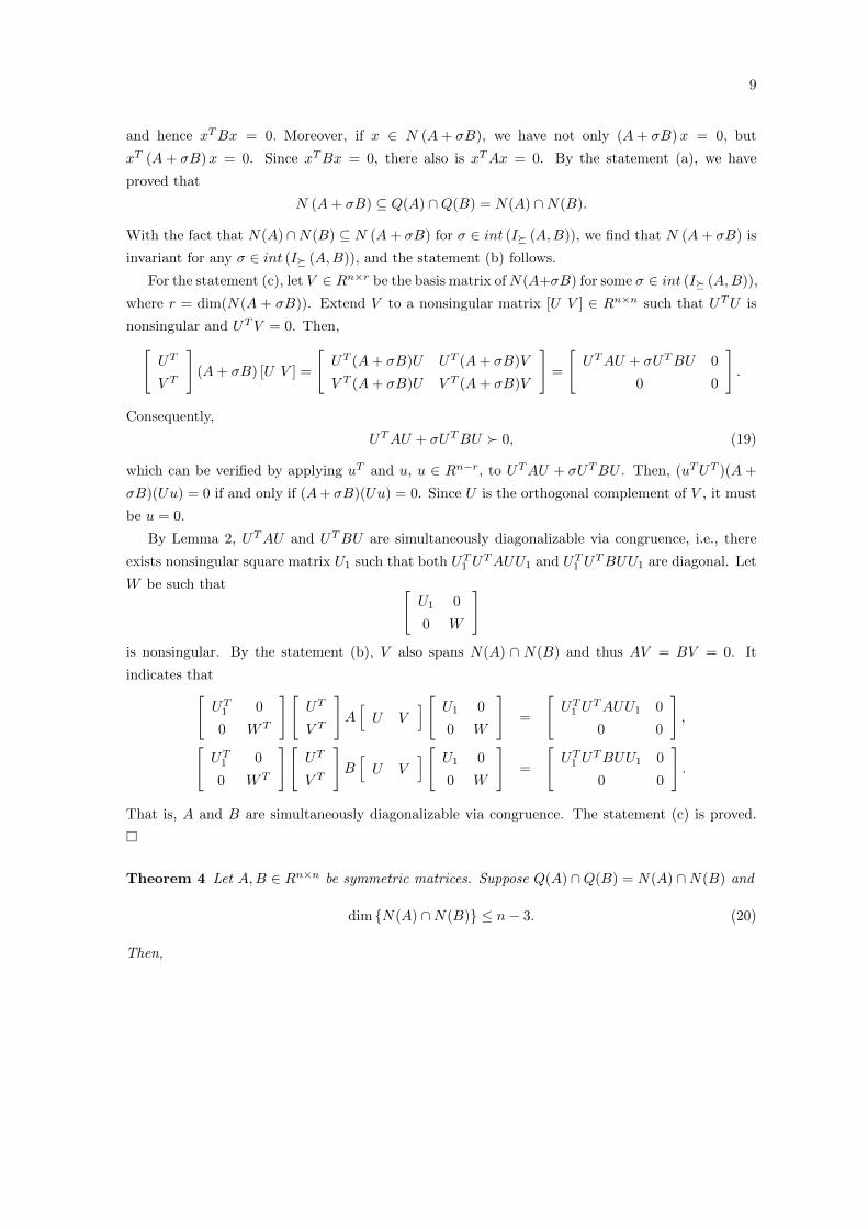
and hence xTBx = 0. Moreover, if x ∈ N (A+ σB), we have not only (A+ σB)x = 0, but
xT (A+ σB)x = 0. Since xTBx = 0, there also is xTAx = 0. By the statement (a), we have
proved that
N (A+ σB) ⊆ Q(A) ∩Q(B) = N(A) ∩N(B).
With the fact that N(A)∩N(B) ⊆ N (A+ σB) for σ ∈ int (I� (A,B)), we find that N (A+ σB) is
invariant for any σ ∈ int (I� (A,B)), and the statement (b) follows.
For the statement (c), let V ∈ Rn×r be the basis matrix ofN(A+σB) for some σ ∈ int (I� (A,B)),
where r = dim(N(A + σB)). Extend V to a nonsingular matrix [U V ] ∈ Rn×n such that UTU is
nonsingular and UTV = 0. Then,[UT
V T
](A+ σB) [U V ] =
[UT (A+ σB)U UT (A+ σB)V
V T (A+ σB)U V T (A+ σB)V
]=
[UTAU + σUTBU 0
0 0
].
Consequently,
UTAU + σUTBU � 0, (19)
which can be verified by applying uT and u, u ∈ Rn−r, to UTAU + σUTBU . Then, (uTUT )(A +
σB)(Uu) = 0 if and only if (A+ σB)(Uu) = 0. Since U is the orthogonal complement of V , it must
be u = 0.
By Lemma 2, UTAU and UTBU are simultaneously diagonalizable via congruence, i.e., there
exists nonsingular square matrix U1 such that both UT1 UTAUU1 and UT1 U
TBUU1 are diagonal. Let
W be such that [U1 0
0 W
]is nonsingular. By the statement (b), V also spans N(A) ∩ N(B) and thus AV = BV = 0. It
indicates that[UT1 0
0 WT
][UT
V T
]A[U V
] [ U1 0
0 W
]=
[UT1 U
TAUU1 0
0 0
],[
UT1 0
0 WT
][UT
V T
]B[U V
] [ U1 0
0 W
]=
[UT1 U
TBUU1 0
0 0
].
That is, A and B are simultaneously diagonalizable via congruence. The statement (c) is proved.
�
Theorem 4 Let A,B ∈ Rn×n be symmetric matrices. Suppose Q(A) ∩Q(B) = N(A) ∩N(B) and
dim {N(A) ∩N(B)} ≤ n− 3. (20)
Then,

10
• (a’) II�(UTAU,UTBU) 6= ∅ where U is the basis matrix spans the orthogonal complement of
N(A) ∩N(B);
• (b’) II�(A,B) 6= ∅; and
• (c’) A,B are simultaneously diagonalizable via congruence.
Proof. Following the same notation in the proof of Theorem 3, we let V ∈ Rn×r be the basis
matrix of N(A) ∩ N(B), r = dim(N(A) ∩ N(B)), and then extend V to a nonsingular matrix
[U V ] ∈ Rn×n such that UTU is nonsingular and UTV = 0. For any x ∈ Q(UTAU) ∩ Q(UTBU),
we have xTUTAUx = xTUTBUx = 0 and thus Ux ∈ Q(A)∩Q(B). By assumption, Q(A)∩Q(B) =
N(A) ∩N(B), there must exist z ∈ Rr such that
Ux = V z.
Therefore,
x = (UTU)−1UTV z = 0,
which shows that
Q(UTAU) ∩Q(UTBU) = {0}. (21)
It follows from Assumption (20) that
dim(UTAU) = dim(UTBU) = n− r ≥ 3.
According to Theorem 1, (21) implies that
II�(UTAU,UTBU) 6= ∅. (22)
Namely, there exists (µ, σ) ∈ R2 such that µ(UTAU) + σ(UTBU) � 0, which proved the statement
(a’). Now, for y ∈ Rn, we can write y = Uu+ V v, where u ∈ Rn−r, v ∈ Rr. Then,
yT (µA+ σB)y
= (uTUT + vTV T )(µA+ σB)(Uu+ V v)
= uT (µUTAU + σUTBU)u ≥ 0,
which proves II�(A,B) 6= ∅. From (22) and Lemma 2, we again conclude that UTAU and UTBU
are simultaneously diagonalizable via congruence. It follows from the same proof for the statement
(c) in Theorem 3 that A,B are indeed simultaneously diagonalizable via congruence. The proof is
complete. �

11
Remark 1 When Q(A)∩Q(B) = {0}, the assumption of Theorem 4 becomes N(A)∩N(B) = {0}.In this case, the dimension condition (20) is equivalent to n ≥ 3 and the basis matrix U is indeed
In, the identical matrix of dimension n. From the statement (a’) in Theorem 4, we conclude that
II�(A,B) 6= ∅. In other words, we have generalized the part of conclusion in Theorem 1 that
“Q(A) ∩Q(B) = {0} and n ≥ 3” implies “II�(A,B) 6= ∅”.
As an immediate corollary of Theorem 4, we obtain sufficient conditions to make A and B
simultaneously diagonalizable via congruence.
Corollary 1 Let A,B ∈ Rn×n be symmetric matrices. Suppose one of the following conditions is
satisfied,
• (S1) I�(A,B) contains more than one point;
• (S2) I�(B,A) contains more than one point;
• (S3) Q(A) ∩Q(B) = N(A) ∩N(B), with dim {N(A) ∩N(B)} 6= n− 2,
then A,B are simultaneously diagonalizable via congruence.
Proof. Conditions (S1) and (S2) directly implies that I�(A,B) (and I�(B,A) respectively) is non-
empty and is not a single point set. The conclusion follows from the statement (c) of Theorem 3.
Condition (S3) is a slight generalization of Theorem 4 where the situation for dim {N(A) ∩N(B)} ≤n− 3 has already been proved. It remains to show that A,B are simultaneously diagonalizable via
congruence when dim {N(A) ∩N(B)} = n ∨ (n − 1). Notice that dim {N(A) ∩N(B)} = n implies
A = B = 0 (in which case the conclusion follows immediately), whereas dim {N(A) ∩N(B)} = n−1
implies that matrices A and B must be expressed as A = αuuT , B = βuuT for some vector u ∈ Rn
and α2 + β2 6= 0. Suppose β 6= 0, then A = αβB so the two matrices are certainly simultaneously
diagonalizable via congruence. �
Example 1 below shows that the non-single-point assumption of I�(A,B) is necessary to assure
statement (a) and (c); and the dimensionality assumption in (S3) is also necessary.
Example 1 Consider
A =
[1 0
0 0
], B =
[0 1
1 0
]. (23)
Then there is only one σ = 0 such that A+ σB � 0, but
Q(A) ∩Q(B) =
{[0
∗
]};
N(A) ∩N(B) = {0} ;
dim {N(A) ∩N(B)} = n− 2.
It is not difficult to verify that here A and B cannot be simultaneously diagonalizable via congruence.
12
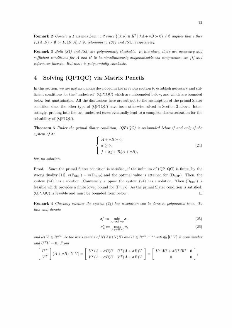
Remark 2 Corollary 1 extends Lemma 2 since {(λ, ν) ∈ R2 | λA+ νB � 0} 6= ∅ implies that either
I�(A,B) 6= ∅ or I�(B,A) 6= ∅, belonging to (S1) and (S2), respectively.
Remark 3 Both (S1) and (S2) are polynomially checkable. In literature, there are necessary and
sufficient conditions for A and B to be simultaneously diagonalizable via congruence, see [1] and
references therein. But none is polynomially checkable.
4 Solving (QP1QC) via Matrix Pencils
In this section, we use matrix pencils developed in the previous section to establish necessary and suf-
ficient conditions for the “undesired” (QP1QC) which are unbounded below, and which are bounded
below but unattainable. All the discussions here are subject to the assumption of the primal Slater
condition since the other type of (QP1QC) have been otherwise solved in Section 2 above. Inter-
estingly, probing into the two undesired cases eventually lead to a complete characterization for the
solvability of (QP1QC).
Theorem 5 Under the primal Slater condition, (QP1QC) is unbounded below if and only if the
system of σ: A+ σB � 0,
σ ≥ 0,
f + σg ∈ R(A+ σB),
(24)
has no solution.
Proof. Since the primal Slater condition is satisfied, if the infimum of (QP1QC) is finite, by the
strong duality [11], v(PSDP) = v(DSDP) and the optimal value is attained for (DSDP). Then, the
system (24) has a solution. Conversely, suppose the system (24) has a solution. Then (DSDP) is
feasible which provides a finite lower bound for (PSDP). As the primal Slater condition is satisfied,
(QP1QC) is feasible and must be bounded from below. �
Remark 4 Checking whether the system (24) has a solution can be done in polynomial time. To
this end, denote
σ∗l := minA+σB�0
σ, (25)
σ∗u := maxA+σB�0
σ, (26)
and let V ∈ Rn×r be the basis matrix of N(A)∩N(B) and U ∈ Rn×(n−r) satisfy [U V ] is nonsingular
and UTV = 0. From[UT
V T
](A+ σB) [U V ] =
[UT (A+ σB)U UT (A+ σB)V
V T (A+ σB)U V T (A+ σB)V
]=
[UTAU + σUTBU 0
0 0
],

13
it can be seen that, if UTBU = 0 and UTAU 6� 0, then I�(A,B) = ∅ and the system (24) has no
solution. It follows that (QP1QC) must be unbounded below in this case.
Assume that I�(A,B) 6= ∅ and σ ∈ I�(A,B). Then, we observe from
A+ σB = (A+ σB) + (σ − σ)B
that σ∗l = −∞ if and only if B � 0. Similarly, σ∗u =∞ if and only if B � 0.
Now suppose −∞ < σ∗l ≤ σ∗u < ∞. From the proof for the statement (c) in Theorem 3 and
(19), if σ ∈ int (I� (A,B)), then UTAU + σUTBU � 0. Conversely, if UTAU + σUTBU � 0, there
must be some ε > 0 such that UTAU + (σ ± ε)UTBU � 0 and thus A + (σ ± ε)B � 0. It holds
that σ ∈ int (I� (A,B)). Consequently, σ∗l and σ∗u, as end points of I� (A,B), must be roots of the
polynomial equation
det(UTAU + σUTBU) = 0. (27)
We first find all the roots of the polynomial equation (27), denoted by r1, . . . , rn−r, which can be
done in polynomial time. Then,
σ∗l = min{ri : UTAU + riUTBU � 0, i = 1, . . . , n− r},
σ∗u = max{ri : UTAU + riUTBU � 0, i = 1, . . . , n− r}.
• Case (a) If σ∗u < 0, (24) has no solution.
• Case (b) σ∗u = 0 or σ∗l = σ∗u > 0. Checking the feasibility of (24) is equivalent to verify
whether the linear equation
(A+ σB)x = f + σg
has a solution for σ = 0 or σ = σ∗l = σ∗u.
• Case (c) σ∗u > 0 and σ∗l < σ∗u. According to Theorem 3, the basis matrix V spans N(A +
σ′B) = N(A) ∩N(B) for any σ′ ∈ (σ∗l , σ∗u).
– Subcase (c1) σ∗l < 0. (24) has a solution if and only if either there is a σ ∈ [0, σ∗u) such
that
V T f + σV T g = 0, (28)
or the linear equation
(A+ σ∗uB)x = f + σ∗ug
has a solution.
– Subcase (c2) σ∗l ≥ 0. (24) has a solution if and only if one of the following three
conditions holds:
V T f + σV T g = 0, for some σ ∈ (σ∗l , σ∗u); (29)
(A+ σ∗l B)x = f + σ∗l g has a solution;
(A+ σ∗uB)x = f + σ∗ug has a solution.

14
We show either (28) or (29) is polynomially solvable. Since V, f, g are fixed, if V T f = V T g = 0,
V T f + σV T g = 0 holds for any σ. If V T f and V T g 6= 0 are linear dependent, there is a unique σ
such that V T f + σV T g = 0. Otherwise, V T f + σV T g = 0 has no solution.
From Theorem 5, it is clear that, if (QP1QC) is bounded from below, the positive semidefinite
matrix pencil I�(A,B) must be non-empty. In solving (QP1QC), we therefore divide into two cases:
I�(A,B) is an interval or I�(A,B) is a singleton.
Theorem 6 Under the primal Slater condition, if the optimal value of (QP1QC) is finite and
I�(A,B) is an interval, the infimum of (QP1QC) is always attainable.
Proof. Let [U V ] ∈ Rn×n be a nonsingular matrix such that V spans N(A) ∩N(B). By Theorem
3, for any σ′ ∈ int (I� (A,B)), V also spans N(A+ σ′B). It follows from (19) that
UTAU + σ′UTBU � 0, ∀σ′ ∈ int (I� (A,B)) . (30)
Since v(QP1QC) > −∞, there is a solution σ to the system (24) such that σ ∈ I�(A,B)∩[0,+∞)
and f + σg ∈ R(A + σB). Since V spans N(A) ∩ N(B), V must span a subspace contained in
N(A+ σB). It follows from f + σg ∈ R(A+ σB) that
V T f + σV T g = 0. (31)
Consider the nonsingular transformation x = Uu + V v which splits (QP1QC) into u-part and
v-part:
min f(u, v) = uTUTAUu− 2fTUu− 2fTV v (32)
s.t. g(u, v) = uTUTBUu− 2gTUu− 2gTV v ≤ µ. (33)
• Case (d) V T f = V T g = 0. Then, (QP1QC) by (32)-(33) is reduced to a smaller (QP1QC)
having only the variable u. Moreover, the smaller (QP1QC) satisfies the dual Slater condition
due to (30). It is hence solvable. See, for example, [15, 25, 7].
• Case (e) V T f = 0, V T g 6= 0. By (31), we have σ = 0 which implies that A � 0 and f ∈ R(A).
In this case, since (33) is always feasible for any u, (32)-(33) becomes an unconstrained convex
quadratic program (32), which is always solvable due to f ∈ R(A).
• Case (f) V T f 6= 0. By (31), V T g 6= 0, σ is unique and nonzero. Thus, σ > 0. Then, the
constraint (33) is equivalent to
σuTUTBUu− 2σgTUu− 2σgTV v ≤ σµ,
or equivalently, by (31),
−2fTV v = 2σgTV v ≥ σuTUTBUu− 2σgTUu− σµ. (34)
15
Therefore, (32)-(33) has a lower bounding quadratic problem with only the variable u such
that
f(u, v) ≥ uT (UTAU + σUTBU)u− 2(fTU + σgTU)u− σµ. (35)
Since A + σB � 0, the right hand side of (35) is a convex unconstrained problem. With
f + σg ∈ R(A + σB), if f + σg = (A + σB)w, we can write w = Uy∗ + V z∗ to make
f + σg = (A + σB)Uy∗ and thus obtain UT (f + σg) ∈ R(UTAU + σUTBU) with y∗ being
optimal to (35). Substituting u = y∗ into (34), due to V T f 6= 0, there is always some v = z∗
such that (u, v) = (y∗, z∗) makes (34) hold as an equality. Then, g(y∗, z∗) ≤ µ and f(y∗, z∗)
attains its lower bound in (35). Therefore, (u, v) = (y∗, z∗) solves (32)-(33).
Summarizing cases (d), (e) and (f), we have thus completed the proof of this theorem. �
What remains to discuss is when the positive semidefinite matrix pencil I�(A,B) is a singleton
{σ∗}. By Theorem 5, (QP1QC) is bounded from below if and only if we must have σ∗ ≥ 0 such
that, with V being the basis matrix of N(A+ σ∗B) and r = dimN(A+ σ∗B), the set
S = {(A+ σ∗B)+(f + σ∗g) + V y | y ∈ Rr} (36)
is non-empty. According to the result (quoted in Introduction) by More in [15], x∗ solves (QP1QC)
if and only if x∗ ∈ S is feasible and (x∗, σ∗) satisfy the complementarity. We therefore have the
following characterization for a bounded below but unattainable (QP1QC).
Theorem 7 Suppose the primal Slater condition holds and the optimal value of (QP1QC) is finite.
The infimum of (QP1QC) is unattainable if and only if I�(A,B) is a single-point set {σ∗} with
σ∗ ≥ 0, and the quadratic (in)equality{g ((A+ σ∗B)+(f + σ∗g) + V y) = µ, if σ∗ > 0,
g (A+f + V y) ≤ µ, if σ∗ = 0,(37)
has no solution in y, where V is the basis matrix of N(A+ σ∗B).
Proof. Since v(QP1QC) is assumed to be finite, by Theorem 5, the system (24) has at least one
solution. By Theorem 6, the problem can be unattainable only when I�(A,B) is a single-point set
{σ∗} with σ∗ ≥ 0. In addition, the set S in (36) can not have a feasible solution which, together
with σ∗, satisfies the complementarity. In other words, the system (37) can not have any solution in
y, which proves the necessity of the theorem. The sufficient part of the theorem which guarantees a
bounded below but unattainable (QP1QC) is almost trivial. �
Remark 5 Under the condition that I�(A,B) is a single-point set, that is, σ∗l = σ∗u in (25)-(26),
we show how (37) can be checked and how (QP1QC) can be solved in polynomial time.
16
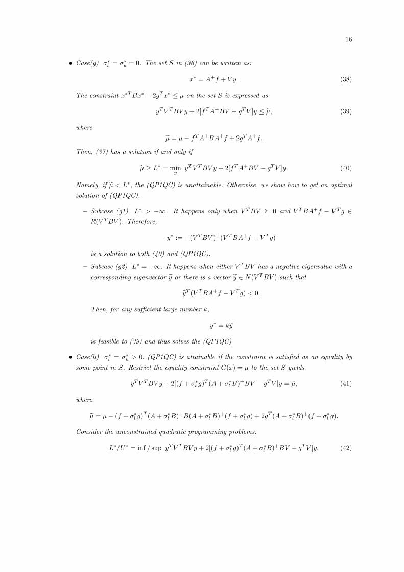
• Case(g) σ∗l = σ∗u = 0. The set S in (36) can be written as:
x∗ = A+f + V y. (38)
The constraint x∗TBx∗ − 2gTx∗ ≤ µ on the set S is expressed as
yTV TBV y + 2[fTA+BV − gTV ]y ≤ µ, (39)
where
µ = µ− fTA+BA+f + 2gTA+f.
Then, (37) has a solution if and only if
µ ≥ L∗ = miny
yTV TBV y + 2[fTA+BV − gTV ]y. (40)
Namely, if µ < L∗, the (QP1QC) is unattainable. Otherwise, we show how to get an optimal
solution of (QP1QC).
– Subcase (g1) L∗ > −∞. It happens only when V TBV � 0 and V TBA+f − V T g ∈R(V TBV ). Therefore,
y∗ := −(V TBV )+(V TBA+f − V T g)
is a solution to both (40) and (QP1QC).
– Subcase (g2) L∗ = −∞. It happens when either V TBV has a negative eigenvalue with a
corresponding eigenvector y or there is a vector y ∈ N(V TBV ) such that
yT (V TBA+f − V T g) < 0.
Then, for any sufficient large number k,
y∗ = ky
is feasible to (39) and thus solves the (QP1QC)
• Case(h) σ∗l = σ∗u > 0. (QP1QC) is attainable if the constraint is satisfied as an equality by
some point in S. Restrict the equality constraint G(x) = µ to the set S yields
yTV TBV y + 2[(f + σ∗l g)T (A+ σ∗l B)+BV − gTV ]y = µ, (41)
where
µ = µ− (f + σ∗l g)T (A+ σ∗l B)+B(A+ σ∗l B)+(f + σ∗l g) + 2gT (A+ σ∗l B)+(f + σ∗l g).
Consider the unconstrained quadratic programming problems:
L∗/U∗ = inf / sup yTV TBV y + 2[(f + σ∗l g)T (A+ σ∗l B)+BV − gTV ]y. (42)

17
We claim that (37) (as well as (QP1QC)) has a solution if and only if µ ∈ [L∗, U∗]. We only
have to prove the “if” part, so µ ∈ [L∗, U∗] is now assumed. Notice that L∗ > −∞ (U∗ < +∞)
if and only if V TBV � (�)0 and V TB(A+ σ∗l B)+(f + σ∗l g)− V T g ∈ R(V TBV ).
– Subcase (h1) L∗ > −∞, U∗ < +∞. This is a trivial case as it happens if and only if
V TBV = 0, V TB(A+ σ∗l B)+(f + σ∗l g)− V T g = 0. Consequently, L∗ = U∗ = 0 and any
vector y is a solution to (37) and solves (QP1QC).
– Subcase (h2) L∗ > −∞, U∗ = +∞. The infimum of (42) is attained at
y = −(V TBV )+[V TB(A+ σ∗l B)+(f + σ∗l g)− V T g].
Furthermore, either V TBV has a positive eigenvalue with a corresponding eigenvector y;
or there is a vector y ∈ N(V TBV ) such that
yT [V TB(A+ σ∗l B)+(f + σ∗l g)− V T g] > 0.
Starting from y and moving along the direction y, we find that
h(α) := (y + αy)TV TBV (y + αy) + 2[(f + σ∗l g)T (A+ σ∗l B)+BV − gTV ](y + αy)
is a convex quadratic function in the parameter α ∈ R with h(0) = L∗. The range of
h(α) must cover all the values above L∗, particularly the value µ ∈ [L∗, U∗]. Then, the
quadratic equation
h(α) = µ
has a root at α∗ ∈ (0,+∞) which generates a solution y∗ = y + α∗y to (41).
– Subcase (h3) L∗ = −∞, U∗ < +∞. Multiplying both sides of the equation (41) by −1,
we turn to Subcase (h2).
– Subcase (h4) L∗ = −∞, U∗ = +∞. Notice that, L∗ = −∞ implies that either V TBV
has a negative eigenvalue with an eigenvector y or there is a vector y ∈ N(V TBV ) such
that
yT [V TB(A+ σ∗l B)+(f + σ∗l g)− V T g] < 0.
Also, U∗ = +∞ implies that either V TBV has a positive eigenvalue with an eigenvector
y or there is a vector y ∈ N(V TBV ) such that
yT [V TB(A+ σ∗l B)+(f + σ∗l g)− V T g] > 0.
Define
h1(α) := yTV TBV yα2 + 2[(f + σ∗l g)T (A+ σ∗l B)+BV − gTV ]yα, (43)
h2(β) := yTV TBV yβ2 + 2[(f + σ∗l g)T (A+ σ∗l B)+BV − gTV ]yβ. (44)

18
where h1(α) is concave quadratic whereas h2(β) convex quadratic. Since h1(0) = h2(0) =
0, the ranges of h1(α) and h2(β), while they are taken in union, cover the entire R.
Therefore, if µ = 0, y∗ = 0 is a solution to (41). If µ < 0, y∗ = α∗y with h1(α∗) = µ is
a solution to (41). If µ > 0, y∗ = β∗y with h2(β∗) = µ is the desired solution.
5 (QP1QC) without SDC
Simultaneously diagonalizable via congruence (SDC) of a finite collection of symmetric matrices
A1, A2, . . . , Am is a very interesting property in optimization due to its tight connection with the
convexity of the cone {(〈A1x, x〉, 〈A2x, x〉, . . . , 〈Amx, x〉)|x ∈ Rn}. See [12] for the reference. In [7],
Feng et al. concluded that (QP1QC) problems under the SDC condition is either unbounded below
or has an attainable optimal solution whereas those having no SDC condition are said to be in the
hard case. In the following, we construct three examples to illustrate why the hard case is complicate.
The examples show that A and B cannot be simultaneously diagonalizable via congruence, while
(QP1QC) could be unbounded below; could have an unattainable solution; or attain the optimal
value.
Example 2 Let
A =
[1 0
0 −1
], B =
[0 1
1 0
], f = g =
[0
0
], µ = 0.
If A and B were simultaneously diagonalizable via congruence, then there would be a nonsingular
matrix P =
[a b
c d
]such that PTAP and PTBP are diagonal matrices. That is,
PTAP =
[a c
b d
][1 0
0 −1
][a b
c d
]=
[a2 − c2 ab− cdab− cd b2 − d2
],
and
PTBP =
[a c
b d
][0 1
1 0
][a b
c d
]=
[2ac ad+ bc
ad+ bc 2bd
]are diagonal matrices. That is, ab − cd = 0, ad + bc = 0, and ad − bc 6= 0 since P is nonsingular.
Since bc = −ad, we have 2ad 6= 0, and hence a, b, c, and d are nonzeros. From ab − cd = 0, we
have a = cdb ; and from ad+ bc = 0, we have a = −bc
d . It implies that cdb + bc
d = 0, which leads to a
contradiction that c(b2 + d2) = 0 and b = d = 0. In other words, A and B cannot be simultaneously
diagonalizable via congruence.
For these A and B, (QP1QC) becomes
(QP1QC) : inf x21 − x2
2
s.t. 2x1x2 ≤ 0.
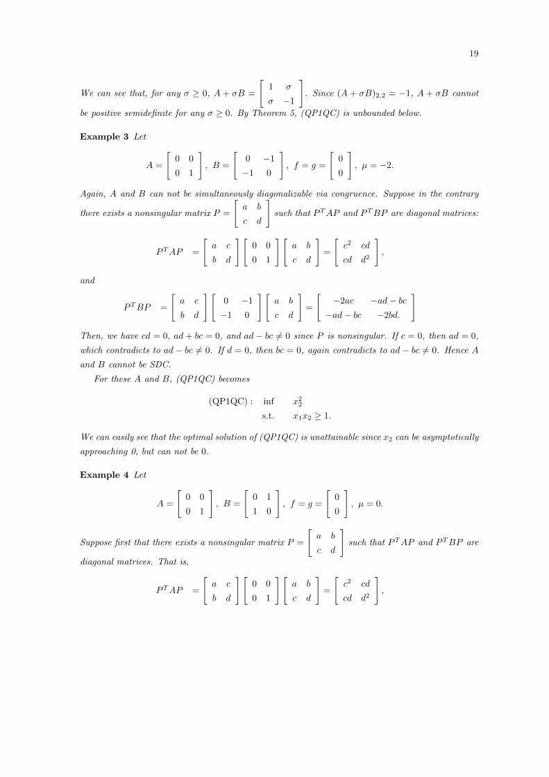
19
We can see that, for any σ ≥ 0, A + σB =
[1 σ
σ −1
]. Since (A + σB)2,2 = −1, A + σB cannot
be positive semidefinite for any σ ≥ 0. By Theorem 5, (QP1QC) is unbounded below.
Example 3 Let
A =
[0 0
0 1
], B =
[0 −1
−1 0
], f = g =
[0
0
], µ = −2.
Again, A and B can not be simultaneously diagonalizable via congruence. Suppose in the contrary
there exists a nonsingular matrix P =
[a b
c d
]such that PTAP and PTBP are diagonal matrices:
PTAP =
[a c
b d
][0 0
0 1
][a b
c d
]=
[c2 cd
cd d2
],
and
PTBP =
[a c
b d
][0 −1
−1 0
][a b
c d
]=
[−2ac −ad− bc−ad− bc −2bd.
]
Then, we have cd = 0, ad+ bc = 0, and ad− bc 6= 0 since P is nonsingular. If c = 0, then ad = 0,
which contradicts to ad− bc 6= 0. If d = 0, then bc = 0, again contradicts to ad− bc 6= 0. Hence A
and B cannot be SDC.
For these A and B, (QP1QC) becomes
(QP1QC) : inf x22
s.t. x1x2 ≥ 1.
We can easily see that the optimal solution of (QP1QC) is unattainable since x2 can be asymptotically
approaching 0, but can not be 0.
Example 4 Let
A =
[0 0
0 1
], B =
[0 1
1 0
], f = g =
[0
0
], µ = 0.
Suppose first that there exists a nonsingular matrix P =
[a b
c d
]such that PTAP and PTBP are
diagonal matrices. That is,
PTAP =
[a c
b d
][0 0
0 1
][a b
c d
]=
[c2 cd
cd d2
],

20
and
PTBP =
[a c
b d
][0 1
1 0
][a b
c d
]=
[2ac ad+ bc
ad+ bc 2bd
]
are diagonal matrices. It follows that cd = 0, ad+ bc = 0, and ad− bc 6= 0 since P is nonsingular.
By bc = −ad, we have 2ad 6= 0, and hence a, b, c, and d are nonzeros, which is contradicts to cd = 0.
Thus A and B cannot be simultaneously diagonalizable via congruence. In this example, (QP1QC)
becomes
(QP1QC) : inf x22
s.t. 2x1x2 ≤ 0
which has the optimal solution set {(x, 0)|x ∈ R}.
6 Conclusions
In this paper, we analyzed the positive semi-definite pencil I�(A,B) for solving (QP1QC) without
any primal Slater condition, dual Slater condition, or the SDC condition. Given any (QP1QC)
problem, we are now able to check whether it is infeasible, or unbounded below, or bounded below
but unattainable in polynomial time. If neither of the undesired cases happened, the solution of
(QP1QC) can be obtained via different relatively simple subproblems in various subcases. In other
words, once a given (QP1QC) problem is properly classified, its solution can be computed readily.
Therefore, we believe that our analysis in this paper has the potential to become an efficient algorithm
for solving (QP1QC) if carefully implemented.
References
[1] R.I. Becker, Necessary and sufficient conditions for the simultaneous diagonability of two
quadratic forms, Linear Algebra and its Applications, 30 129–139 (1980)
[2] A. Ben-Tal and M. Teboulle, Hidden convexity in some nonconvex quadratically constrained
quadratic programming, Mathematical Programming 72, 1996, 51-63.
[3] S. Boyd, L. El Ghaoui, E. Feron, and V. Balakrishnan, Linear Matrix Inequalities in System
and Control Theory. Society for Industrial and Applied Mathematics, 1994.
[4] S. Boyd and L. Vandenberghe. Convex Optimization. Cambridge University Press, 2003.
[5] S.C. Fang, G.X. Lin, R.L. Sheu and W. Xing, Canonical dual solutions for the double well
potential problem, preprint.

21
[6] G. C. Fehmers, L. P. J. Kamp, and F. W. Sluijter, An algorithm for quadratic optimization
with one quadratic constraint and bounds on the variables. Inverse Problems, 14, 1998, 893-901.
[7] J.M. Feng, G.X. Lin, R.L. Sheu and Y. Xia, Duality and Solutions for Quadratic Programming
over Single Non-Homogeneous Quadratic Constraint, Journal of Global Optimization, Vol. 54,
2012, 275 - 293.
[8] C. Fortin and H. Wolkowicz, The trust region subproblem and semidefinite programming. Op-
timization Methods and Software. 19(1), 2004, 41-67.
[9] D. M. Gay, Computing optimal locally constrained steps. SIAM J. Sci. Stat. Comput., 2(2),
1981, 186-197.
[10] G. H. Golub and U. Von Matt, Quadratically constrained least squares and quadratic problems.
Numerische Mathematik, 59, 1991, 186-197.
[11] C. Helmberg. Semidefinite programming. European Journal of Operational Research, 137(3),
2002, 461-482.
[12] J.-B. Hiriart-Urruty, Potpourri of conjectures and open questions in nonlinear analysis and
optimization. SIAM Review, 49(2), 2007, 255-273.
[13] R. Horn and C.R. Johnson, Matrix analysis. Cambridge University Press, Cambridge, UK, 1985.
[14] J.M. Martınez, Local minimizers of quadratic functions on euclidean balls and spheres. SIAM
J. Optimization, 4, 1994, 159-176.
[15] J.J. More, Generalizations Of The Trust Region Problem, Optimization Methods and Software,
2, 1993, 189-209.
[16] J.J. More and D.C. Sorensen, Computing a trust region step. SIAM J. Sci. Statist. Comput.,
4, 1983, 553-572.
[17] Y. Nesterov and A. Nemirovsky, Interior-point polynomial methods in convex programming,
SIAM, Philadelphia, PA, 1994.
[18] I. Polik and T. Terlaky, A survey of the S-lemma. SIAM Review, 49(3), 2007, 371-418.
[19] N. Shor, Quadratic optimization problems. Sov. J. Comput. Syst. Sci., 25: 1–11 (1987)
[20] R.J. Stern and H. Wolkowicz, Indefinite trust region subproblems and nonsymmetric perturba-
tions. SIAM J. Optim., 5(2), 1995, 286-313.
[21] J.F. Sturm and S. Zhang, On cones of nonnegtive quadratic functions. Mathematics of Opera-
tions Research, 28(2), 2003, 246-267.
22
[22] F. Uhlig, A recurring theorem about pairs of quadratic forms and extensions: A survey, Linear
Algebra Appl., 25, 1979, 219-237.
[23] L. Vandenberghe and S. Boyd, Semidefinite programming, SIAM Review 38, 1996, 49-95.
[24] W. Xing, S.C. Fang, D.Y. Gao, R.L. Sheu and L. Zhang, Canonical dual solutions to the
quadratic programming over a quadratic constraint, submitted.
[25] Y. Ye and S. Zhang, New results on quadratic minimization. SIAM J. Optim., 14(1), 2003,
245-267.


![arXiv:2012.14550v1 [math.PR] 29 Dec 2020 · arXiv:2012.14550v1 [math.PR] 29 Dec 2020 Quadratic Transportation Cost Inequality For Scalar Stochastic ConservationLaws Rangrang Zhang1,](https://cdn.vdocuments.net/doc/165x107/610291840fd9ec09fb472cad/arxiv201214550v1-mathpr-29-dec-2020-arxiv201214550v1-mathpr-29-dec-2020.jpg)

