
Journal of Mechanical Science and Technology 23 (2009) 1157~1168 www.springerlink.com/content/1738-494x
DOI 10.1007/s12206-009-0305-8
Journal of Mechanical Science and Technology
A study on reliability centered maintenance planning of a standard
electric motor unit subsystem using computational techniques† Chulho Bae1, Taeyoon Koo1, Youngtak Son1, Kyjun Park2, Jongdeok Jung2,
Seokyoun Han2 and Myungwon Suh3,* 1Graduate School of Mechanical Engineering, Sunkyunkwan University, Suwon, 440-746, Korea
2Urban Transportation R&D Center, Korea Railroad Research Institute, Uiwang, 437- 757, Korea 3School of Mechanical Engineering, Sunkyunkwan University, Suwon, 440-746, Korea
(Manuscript Received February 21, 2008; Revised March 10, 2009; Accepted March 19, 2009)
--------------------------------------------------------------------------------------------------------------------------------------------------------------------------------------------------------------------------------------------------------
Abstract The design and manufacture of urban transportation applications has been necessarily complicated in order to im-
prove its safety. Urban transportation systems have complex structures that consist of various electric, electronic, and mechanical components, and the maintenance costs generally take up approximately 60% of the total operational costs. Therefore, it is essential to establish a maintenance plan that takes into account both safety and cost. In considering safety and cost limitations, this research introduces an advanced reliability centered maintenance (RCM) planning method using computational techniques, and applies the method to a standard electric motor unit (EMU) subsystem. First, this research devises a maintenance cost function that can reflect the current operating conditions, and mainte-nance characteristics, of components by generating essential cost factors. Second, a reliability growth analysis (RGA) is performed, using the Army Material Systems Analysis Activity (AMSAA) model, to estimate reliability indexes such as failure rate, and mean time between failures (MTBF), of a standard EMU subsystem, and each individual component Third, two optimization processes are performed to ascertain the optimal maintenance reliability of each component in the standard EMU subsystem. Finally, this research presents the maintenance time of each component based on the optimal maintenance reliability provided by optimization processesand reliability indexes provided by the RGA method.
Keywords: Failure rate; Maintenance cost function; Maintenance reliability allocation; Maintenance plan; Mean time between failures;
Reliability centered maintenance; Reliability growth analysis; Urban transportation systems --------------------------------------------------------------------------------------------------------------------------------------------------------------------------------------------------------------------------------------------------------
1. Introduction
The design and manufacture of urban transporta-tion systems have been necessarily complicated in order to improve their safety. For this reason, urban transportation systems have complex structures that consist of various electric, electronic, and mechanical components, and the maintenance costs generally take up approximately sixty percent of the total operation
costs [7]. Therefore, an urban transportation based society requires a reliable maintenance structure that can maintain a high level of functionality, without a critical failure, and can also reduce the maintenance costs.
In considering both safety and cost limitations, this research introduces the concept of ‘reliability’ and reliability centered maintenance (RCM). In general, RCM is a systematic approach used to establish a cost-effective maintenance strategy based on the vari-ous components’ reliability of the system in question [11, 14], and reliability is defined as, the probability that an item will perform a required function without
†This paper was recommended for publication in revised form by Associate Editor Dae-Eun Kim
*Corresponding author. Tel.: +82 31 290 7447, Fax.: +82 31 290 5889 E-mail address: [email protected] © KSME & Springer 2009

1158 C. Bae et al. / Journal of Mechanical Science and Technology 23 (2009) 1157~1168
failure under stated conditions for a stated period of time [4]. This concept can be adapted, and applied to urban transit, in order to establish an efficient mainte-nance plan for supporting each subsystem.
There have been many studies following the pro-gress of RCM. Smith [14] defined RCM as a method to determine any reliable operations for physical equipment, and presented a preventive maintenance plan by analyzing functional failures. Richard [11] introduced a practical method of applying the RCM technique, which Smith et al. had presented, to the industrial field. Jacobs [6] studied this method, which reduced maintenance tasks by its use of the RCM. In the field of railway maintenance and safety, the pre-ventive diagnosis, and the predictive maintenance, for railway equipment was studied by Wada [15]. More recently, Mettas [8] demonstrated that optimization methods could minimize the operating function and still satisfy the target system. However, further re-search on the maintenance data and the optimization performance using a quantitative approach for the maintenance phase, is still necessary. This research introduces an advanced RCM planning method using computational techniques and applies the method to urban transit by using a standard electric motor unit (EMU).
The proposed RCM planning method comprises two optimization steps. The first step uses the reliabil-ity matrix to minimize the total maintenance cost while, at the same time, maximize the subsystem reliability. This is achieved by using a multi-objective optimization method. From this the maintenance cost function can reflect the current maintenance charac-teristics of the components by generating essential cost factors defined by the reliability, and maintain-ability, of each component. In addition, this research defines the reliability function of the EMU subsystem by using a reliability network, between appropriate subsystems and components, which mimic an artifi-cial neural network. The second optimization step allocates the maintenance reliability of each compo-nent to the maintenance cost, reliability function, and desired subsystem reliability. In the case of mainte-nance reliability allocation, the optimisation process seeks to minimize the maintenance costs whilst meet-ing the desired subsystem reliability requirements. This research applies an evolutionary algorithm to find the best reliability allocation by searching for the global optimum in the nonlinear domain. Finally, the paper presents an effective maintenance plan, deter-
mined by estimating the maintenance time of the components as derived from the allocated reliability, and reliability indexes, in the inverse analysis of the fundamental reliability function.
2. RCM-based maintenance optimization
This research allocates suitable maintenance reli-ability values to each component by using optimiza-tion techniques. The optimization is used to minimize the maintenance costs, and also to meet the desired reliability requirements of the overall system. There-fore, the optimization problem can be expressed as shown in Eq. (1).
1 : ( )
n
i iR i
Minimize C C R=
=∑
g s
i,min i i,max
: ( ),
1 2
iSubject to R R R
R R Ri , ,.....,n
≤
≤ ≤=
(1)
where , *( )g sR R t= where, C = the total system maintenance cost, n = the number of components, iC = the maintenance cost of the i -th component, iR = the reliability of the i -th component, sR = the system reliability, gR = the desired system reliability, ,maxiR = the maximum reli-ability of the i -th component, and ,miniR = the mini-mum reliability of the i -th component. The inequality constraint is the desired system reliability, gR , which is derived from asub-optimization process as shown in Eq. (2).
*
: ( ): ( )
: 0s
s t t
Minimize C tMaximize R tSubject to t m
=
⎛ ⎞⎜ ⎟⎝ ⎠
≤ ≤ (2)
Where, t = the whole operating time, which means independent variables, 0t = the point of re-pair/exchange time, and sm = the system MTBF.
This demonstrates the probability of a system main-taining a function, without failure, during a desired period of time. The system reliability, ( )s iR R , has been calculated by using equations based on the reli-ability relationship (reliability block diagram (RBD)) between a system and its members. However, this conventional method of calculating the system reli-ability can be difficult to apply as it is almost impossi-ble to construct and define the reliability relationship

C. Bae et al. / Journal of Mechanical Science and Technology 23 (2009) 1157~1168 1159
between a system and its components when used in actual complex structures such as urban transit. In view of this, we propose to use an approximation me-thod to calculate the system reliability. Therefore, our research constructs the relationship through an artifi-cial technique based on neural networks and using approximation methods.
The reliability of each component, iR , is used as the design variables, and its scope is limited by the side constraint condition. The maximum reliability that can be achieved is 0.999, and the minimum reliability is individually determined by the appropriate charac-teristic factors. These factors are estimated by critical-ity analyzing the degree to which system function is affected when a component fails, and the func-tional/structural importance of the component in the system. Thus, as the importance and criticality of a component increases, the minimum required reliabil-ity also increases.
3. Maintenance cost function
In this section we derive the total maintenance cost function of a system with many components. Assum-ing that the total cost is the sum of the operational costs of the individual components, then the system operational cost can be defined as the sum of the initial cost, repair of cost, and the overall management costs. The total cost function can be expressed as shown in Eq. (3).
1 ( )
n
initial repair managei
Total cost(c) C C C=
= + +∑ (3)
Where, initialC = the initial cost function, repairC = the repair cost function, manageC = the management cost function.
Each cost function is defined as follows: First, the initial cost is the total value of the purchase
through to installation, which can be shown as Eq. (4).
11
n
initial i ii
C w n=
=∑ (4)
Where, 1iw = the initial cost weight factor of the i-th component, and n = the number of components.
Second, the individual component repair cost is an approximated cost for repairing failures of each com-ponent (e.g., the i-th component) [12]. This does not
include any costs associated with failures which are not caused by breakdown of the i-th component. The total system repair cost is then obtained as the sum of the individual costs of each component and can be written as Eq. (5).
( )21
(1 )n
repair i s i ii
C w R k R=
= × × −∑ (5)
Where, 2iw = the repair cost weight factor of the i-th component, n = the number of components, and
ik =the redundancy number of the i-th component. Third, the management cost is the total cost of
maintaining, or improving, reliability, as illustrated by Eq. (6) [1].
,min3
1 ,max
ˆ exp (1 )n
i imainte i i i
i i i
R RC w k m
R R=
⎛ ⎞⎛ ⎞−= ⎜ × − ⎟⎜ ⎟⎜ ⎟⎜ ⎟−⎝ ⎠⎝ ⎠∑ (6)
Where, ˆ im = the maintainability of the i-th component. The maintainability of a component is the ease by which a component can be modified to correct faults or improve performance. The maintainability ˆ im is expressed in Eq. (7). In this, the mean time to repair (MTTR) is defined as the average time a component will take to recover from a non-terminal failure, and can be obtained by analyzing historical failure data.
1ˆ expim t
MTTR⎛ ⎞= − ×⎜ ⎟⎝ ⎠
(7)
Where, t = the elapsed operation time.
The maintenance cost function complies with the following rules: 1) the cost of maintaining the desired level of reliability for a component is very high, 2) the cost of maintaining a low level of reliability for a component is very low, and 3) the curve of the main-tenance cost function increases in direct proportion to the required reliability of a component, as can be seen in Fig. 1. In the region where reliability is low, the maintenance cost is also low, and its slope seems to be almost uniform. In contrast, in the region where reli-ability is high, the maintenance cost is increased by the increase in reliability. Notice that in the region where reliability is greater than 0.95, an exponential growth of the maintenance cost value is seen. Fig. 1 also shows the effect of ˆ im in the maintenance cost func-tion where ˆ im has a value ranging from 0 to 1, and when ˆ im equals 1, the maintainability of the i -th

1160 C. Bae et al. / Journal of Mechanical Science and Technology 23 (2009) 1157~1168
component is 100%. Although some components have the same reliability, a component having a high ˆ im has a higher maintenance cost than a component hav-ing low ˆ im .
4. Sample model definition - door & door con-trol system
This research applies the proposed RCM method to a variable voltage variable frequency (VVVF) EMU subsystem. The proposed RCM method requires a model definition, such as bill of materials (BOM) and/or function block diagram (FBD), and operation data. This paper describes the application of the pro-posed RCM method, by taking a door and door con-trol (DDC) system as a sample model as this system has the highest failure rate out of fourteen standard
Fig. 1. The effect of ˆ im , iR in maintenance cost function.
EMU subsystems. The operational data contains historical failure data
of each component, obtained over a period of 5 years (2000~’04), and is composed of the failed part com-ponent code, cumulative failure number, and opera-tional time. The operational data is based on two sup-positions: first, that the components are not exchanged for 5 years, and second, if the components are repaired because of failure, their functionality is restored to their original 100% reliability.
A DDC system is composed of a passenger door, a driver door, and an aisle door. Failures in the driver or an aisle door show simple failure modes such as wear, corrosion, and cracking, because they consist of a mechanical rocking device and a door panel. There-fore, we construct a model for the passenger door hav-ing electric and mechanical characteristics, as these are important to secure both reliability and safety.
A DDC system consists of 5 main components: cylinder, magnetic valve, belt assembly, door panel, and door control device. The primary functional fail-ures of a DDC system are due to piston cap wear, cylinder leakage due to pollution of the head part, magnetic valve breakdown due to oil leakage and the damage caused as a result of the leakage, belt assem-bly damage due to wear, deformation of the door panel, etc. These primary functional failures lead to the breakdown of a DDC system and, hence, affect the operation of a standard EMU. Therefore, the reli-ability is affected by the cylinder, the magnetic valve, belt assembly, the door panel, and the door controller. The functional block diagram (FBD) and historical
Fig. 2. A functional block diagram of a DDC system.
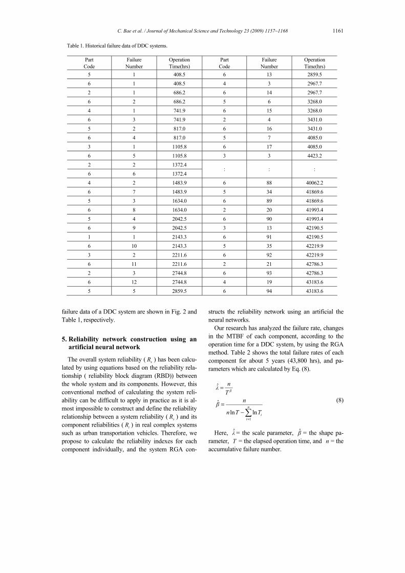
C. Bae et al. / Journal of Mechanical Science and Technology 23 (2009) 1157~1168 1161
failure data of a DDC system are shown in Fig. 2 and Table 1, respectively.
5. Reliability network construction using an artificial neural network The overall system reliability ( sR ) has been calcu-
lated by using equations based on the reliability rela-tionship ( reliability block diagram (RBD)) between the whole system and its components. However, this conventional method of calculating the system reli-ability can be difficult to apply in practice as it is al-most impossible to construct and define the reliability relationship between a system reliability ( sR ) and its component reliabilities ( iR ) in real complex systems such as urban transportation vehicles. Therefore, we propose to calculate the reliability indexes for each component individually, and the system RGA con-
structs the reliability network using an artificial the neural networks.
Our research has analyzed the failure rate, changes in the MTBF of each component, according to the operation time for a DDC system, by using the RGA method. Table 2 shows the total failure rates of each component for about 5 years (43,800 hrs), and pa-rameters which are calculated by Eq. (8).
1
ˆ
ˆln ln
β
n
ii
nλT
nβn T T
=
=
=−∑
(8)
Here, λ̂ = the scale parameter, β̂ = the shape pa-
rameter, T = the elapsed operation time, and n = the accumulative failure number.
Table 1. Historical failure data of DDC systems.
Part Code
Failure Number
Operation Time(hrs)
Part Code
Failure Number
Operation Time(hrs)
5 1 408.5 6 13 2859.5
6 1 408.5 4 3 2967.7
2 1 686.2 6 14 2967.7
6 2 686.2 5 6 3268.0
4 1 741.9 6 15 3268.0
6 3 741.9 2 4 3431.0
5 2 817.0 6 16 3431.0
6 4 817.0 5 7 4085.0
3 1 1105.8 6 17 4085.0
6 5 1105.8 3 3 4423.2
2 2 1372.4
6 6 1372.4 : : :
4 2 1483.9 6 88 40062.2
6 7 1483.9 5 34 41869.6
5 3 1634.0 6 89 41869.6
6 8 1634.0 2 20 41993.4
5 4 2042.5 6 90 41993.4
6 9 2042.5 3 13 42190.5
1 1 2143.3 6 91 42190.5
6 10 2143.3 5 35 42219.9
3 2 2211.6 6 92 42219.9
6 11 2211.6 2 21 42786.3
2 3 2744.8 6 93 42786.3
6 12 2744.8 4 19 43183.6
5 5 2859.5 6 94 43183.6

1162 C. Bae et al. / Journal of Mechanical Science and Technology 23 (2009) 1157~1168
The failure rates of each component are analyzed by applying parameters ( β , λ ) to Eq. (9) and the results are illustrated in Figs. 3-4.
1 11 ,β βc cm T λ λT
λ− −= = (9)
Where, cm = the cumulative MTBF and cλ = the cumulative failure rate.
Fig. 3 shows that the historical failure rate assumes the form of a bath-curve and converges into a unique constant. The convergent values of Fig. 3, give the failure rates of each component at the current op-
Table 2. Analysis results of DDC subsystems using the AMSAA model.
Part Time ln_t Failure Number β̂ λ̂
Cylinder 37,973 10.5446 6 0.994684 0.000167
Magnet valve 42,786 10.6639 21 0.834487 0.002867
Belt ass’y 42,190 10.6499 13 0.784095 0.003071
Door panel 43,183 10.6732 19 0.856501 0.002035
Door control 42,219 10.6506 35 0.777023 0.008911
Fig. 3. Historical failure rates for each component of the DDC system.

C. Bae et al. / Journal of Mechanical Science and Technology 23 (2009) 1157~1168 1163
erating time. The values are: for the cylinder 6158 10Cylλ −= × , for the magnetic valve
6491 10MVVλ −= × , for the belt assem-bly 6308 10Beltλ −= × , for the door panel
6440 10Leafλ −= × , and for the door control-ler 6829 10Conλ −= × . In case of MTBF, the respective convergence values in Fig. 4 are 6,328Cylm = ,
2,037MVVm = , 3,245Beltm = , 2,273Leafm = , 1,206Conm = . The result is shown in Table 3, which
also reiterates the result that the error rate is the mean 1.78% when comparing our result with the reliability analysis result [7] based on MIL-HDBK-217F. The reliability change graph of a DDC system based on the reliability index, such as the failure rate and MTBF, is shown in Fig. 5. At the current time, Fig. 5 shows that the door panel, out of the five components considered,
has been having the lowest breakdown probability, and the door controller has been having the highest gradient of reliability reduction.
We can conclude that a DDC system needs a more powerful preventive maintenance strategy than one simply based on MTBF. This is due to the fact that the MTBF (449 hrs/vehicle) does not meet the re-quired 719 hrs/vehicle [7] maintenance regulations for urban transportation vehicles. It is straightforward to realize the relationship between the reliability of each component and the whole DDC system, at the same time, by using the result illustrated in Table 3. This is used for training the neural network; the reli-abilities of the 5 components which comprise the input layer, and the reliability of a DDC system is the target layer.
Fig. 4. Historical MTBF for each component of the DDC system.

1164 C. Bae et al. / Journal of Mechanical Science and Technology 23 (2009) 1157~1168
Fig. 5. Predicted reliability for each component of the DDC subsystem.
(a) History of neural network training
(b) Comparison of target value with network output value
Fig. 6. Neural network training results.
We extracted the reliability data for a DDC system and the 5 components from the reliability change graph over a period of 449 hrs. The number of the extracted reliability data points was 1,024 for all the various operating times. The number of neurons in the hidden layer used was 10. The neural network was trained for 100,000 iterations by using 1,024 patterns according to various operating times. During training of the neural network, the error rate was 0.001, and the learning rate was 1.05.
The neural network training result between the tar-get value and output value is shown in Fig. 6. The final Sum Square Error (SSE) of the trained neural network was 2.569E-3. It can be verified that the relative error rate between the output value and target value was a very small value, which confirms that the training result of the neural network was good.
6. Maintenance time estimation using evolu-tionary algorithm Fig. 7 shows the optimization flow for the estima-
tion of the proper maintenance time. The optimal reliability is allocated to individual components by using an evolutionary algorithm within the range satisfying the desired system reliability. The tech-nique can search a flexible optimum in the nonlinear domain. The neural network can be trained to find the solution of a nonlinear problem, and the evolutionary algorithm can find the global minimum of a compli-cated optimisation problem. Finally, this research estimates the proper maintenance time that uses the optimal reliability, and reliability indexes, from the inverse analysis of the fundamental reliability func-tion. This research allocates the maintenance reliabil-ity of each component, as was defined in chapter 4, through two optimization processes.
Table 3. Current failure rates & MTBF estimations of a DDC system.
Developed system Reference(KRRI report) Part
Failure rate MTBF(hr) Failure rate MTBF (hr) Error (%)
Cylinder 158 E-6 6,328 155 E-6 6,452 1.94
Magnet valve 491 E-6 2,037 486 E-6 2,057 1.03
Belt ass’y 308 E-6 3,245 301 E-6 3,322 2.33
Door panel 440 E-6 2,273 449 E-6 2,227 2.01
Door control 829 E-6 1,206 816 E-6 1,225 1.59
DDC 2,226 E-6 449 2,208 E-6 453 0.82

C. Bae et al. / Journal of Mechanical Science and Technology 23 (2009) 1157~1168 1165
Fig. 8. The maintenance cost and DDC system reliability sR vs. t .
6.1 Determination of the desired subsystem reliabil-
ity (step 1) The change of the maintenance cost and the sub-
system reliability, according to the operating time, t , is shown in Fig. 8. The values were defined as a func-tion by approximating into the polynomial. The opti-mization problem for determining the desired subsys-tem reliability is defined as follows:
( )( )
*
: ( ) 110.1exp 0.04331
24.51exp 0.002247: ( ) 99.82exp( 0.002204 )
: 0 449DDC
t t
Minimize C t t
tMaximize R t t
Subject to t =
⎛ = − × ⎞⎜ ⎟
+ − ×⎜ ⎟⎜ ⎟⎜ ⎟= − ×⎝ ⎠
≤ ≤
(10)
Where, ( )C t = the maintenance cost function accord-ing to the operating time t , ( )DDCR t = the subsystem reliability function according to the operating time t , and *t = the optimal operating time. The scope of the operating time t is from 0 to the subsystem MTBF (449 hrs).
The optimal operating time *t was obtained through a neighborhood cultivation genetic algorithm (NCGA). For determining the optimal operating time out of many optimum values in a multi-objective problem, we defined the weighting factor of objective functions (the maintenance cost and the system reli-ability function) as 0.5, respectively, because they have the same scale values and both of them are im-portant for this research. As a result, the reliability values at the optimal operating time *t were
CylR =0.9873, MVVR =0.9607, BeltR =0.9755, LeafR =0.9651, ConR =0.9353, and DDCR =0.8356,
which is the desired subsystem reliability. Therefore, this research set up the desired subsystem reliability to 83.56%
6.2 Maintenance reliability allocation (step 2)
The optimization problem (step 2) can be expressed as shown in Eq. (11) by using the desired subsystem reliability obtained by step 1. The design variables are the reliability of each component, eg. CylR , MVVR ,
BeltR , LeafR , and ConR . The objective function is the maintenance cost function as stated in section 3,
Fig. 7. The optimization flow for estimation of the proper maintenance time.

1166 C. Bae et al. / Journal of Mechanical Science and Technology 23 (2009) 1157~1168
which also acts as the fitness function of the evolu-tionary algorithm. In constraints, the subsystem target reliability is determined as 0.8356, every ,maxiR is 0.999 and ,miniR are 0.93, 0.7983, 0.8681, 0.8171, and 0.6835, respectively. To complete the cost func-tion, we have to determine the constant values. The constant values are the weight factor of each cost of the cost function and maintainability. To focus on the effect of the reliabilities, we used the weight factor and maintainability set up to constant 1.
: R
Minimize C = ( )1 21 1
(1 )n n
i i s ii i
w w R R= =
+ × × −∑ ∑
,min3
1 ,max
exp (1 )n
i ii i
i i i
R Rw m
R R=
⎛ ⎞⎛ ⎞−+ ⎜ × − ⎟⎜ ⎟⎜ ⎟⎜ ⎟−⎝ ⎠⎝ ⎠∑
DDC
MVV
Belt
Leaf
: 0.8356, 0 93 0 999
0.7983 0.999 0.8681 0.999 0.8171 0.999 0.81
Cyl
Subject to R. R .
RRR
≥≤ ≤
≤ ≤≤ ≤≤ ≤
Con71 0.999 ( i 1, 2, 3, 4,5)
R≤ ≤=
(11)
The evolutionary algorithm for this research was
set up as follows: population size was 100, crossover rate cp was 0.25, and mutation rate mp was 0.01. Each parameter was represented as a 25-bit binary number, and a roulette wheel selection method was adopted for the selection process. We can estimate the DDC subsystem reliability sR from a trained reli-ability network as defined in section 5.
Table 4 shows the converged reliability results of each component by using the evolutionary algorithm.
We can keep a check on convergence at the 48-rd iteration from the total of 100 iterations. The esti-mated subsystem reliability (0.8356), obtained by using the optimized reliability of each component, satisfied the desired subsystem reliability (0.8356), and reliability of the 5 components, individually, also satisfied the side constraints.
To compare the results, we also added the results of 2 cases (normal step and step 1) in Table 4. Although the DDC subsystem structure was the same, its main-tenance cost values were different according to each step due to the components’ maintenance reliabilities. Put another way, in the case of the normal step with-out reliability allocation, the reliabilities of each com-ponent are 0.9924, 0.9767, 0.9853, 0.9791, and 0.9610, which satisfies DDC subsystem reliability of 0.9 (90 %; typical target reliability), and the value of the objective function (DDC subsystem cost function) is equal to 37.94. For the applied optimal operating time *t , obtained by using only step 1, the reliabil-ities of each component are 0.9873, 0.9607, 0.9755, 0.9651, and 0.9353. In this case, the values of the objective functions (DDC subsystem cost function and the desired reliability) are equal to 25.69 and 0.8356, respectively. In the case of using step 2, the reliabilities of each component are 0.9894, 0.9967, 0.9761, 0.9626, and 0.9312, which satisfies DDC subsystem reliability of 0.8356 (83.56 %; determined by step 1), and the value of the objective function is equal to 25.32.
When this value (25.32) is compared with the nor-mal step (37.94), we can see that 23.25 % mainte-nance cost can be saved by using the proposed RCM method. Finally, the optimal maintenance time of each component can be acquired by substituting the
Table 4. The optimization results.
Components
CylR MVVR BeltR LeafR ConR Rs Cost
Reliability 0.9924 0.9767 0.9853 0.9791 0.9610 Normal (Rs=0.90) Maintenance
Time(hrs) 47.99 0.9000 37.94
Reliability 0.9873 0.9607 0.9755 0.9651 0.9353 Multi-Opt. (step 1) Maintenance
Time(hrs) 80.69 0.8356 25.69
Reliability 0.9894 0.9667 0.9761 0.9626 0.9312 Reli-Opt. (step 2) Maintenance
Time(hrs) 67.45 68.98 78.54 86.63 85.98 0.8356 25.32
Cost reduction Step 1 vs Normal : 22.29 % Step 2 vs Normal: 23.25 %

C. Bae et al. / Journal of Mechanical Science and Technology 23 (2009) 1157~1168 1167
optimized reliability and the current failure rate esti-mated from RGA. The optimal maintenance time is shown in Table 4.
7. Conclusion To consider both safety and cost limitations, this
paper has introduced an advanced RCM planning method using computational techniques, and applied the method to urban transportation systems, in par-ticular, to a standard EMU subsystem. The main con-cept of the proposed RCM method is the optimization of the RCM-based maintenance time.
To construct an RCM-based optimization problem, we first constructed the maintenance cost function, which can reflect the current operating conditions and the maintenance characteristic of the main compo-nents by generating essential cost factors. Second, the RGA method, together with the AMSAA model, was used to estimate reliability indexes, such as failure rate and MTBF, of a standard EMU subsystem and each component. Third, two optimization processes were constructed to allocate the optimal maintenance reliability of each component in a standard EMU subsystem. Finally, we presented a reasonable main-tenance time of each component, based on the allo-cated reliability shown by the optimization problem and reliability indexes by an RGA method.
As a result of the application to a DDC subsystem of a standard EMU, 23.25% of maintenance costs were saved when comparing the final optimization result with a normal step. This saving indicates that the maintenance works have been carried uniformly, without reflecting the system operation conditions and the characteristics of individual components.
In conclusion, this research has presented a useful methodology for obtaining an effective maintenance plan while considering both safety and economical efficiency. These two factors are essential conditions in constructing and maintaining a reliable system, and their importance is ever increasing when used in com-plex modern systems such urban transportation. Therefore, we hope that the new method presented will be a valuable tool for obtaining an effective maintenance plan.
Acknowledgment
This work was supported by the second Brain Ko-rea 21 project and Research & Development on the
Standardization of Urban Railway Transit System.
References
[1] M. Adamantios, Reliability and Optimization for Complex Systems, Proceedings Annual Reliability and Maintainability symposium, (2000) 216-221.
[2] S. E. Fahlman and C. Lebiere, 1990, The cascade-correlation learning architecture, Advances in Neu-ral Information Processing Systems II, Morgan Kaufmann, (1990).
[3] L. J. Fogel, A. J. Owens and M. J. Walsh, Artificial intelligence through simulated evolution, Wiley Publishing, New York, (1966).
[4] F. P. Garcia Marquez, F. Schnid and J. C. Collado, A reliability centered approach to remote condition monitoring, Reliability Engineering and System Safety, (1993) 33-40.
[5] J. H. Holland, Adaptation in natural and artificial systems, The University of Michigan Press, Ann Arbor, Michigan, (1975).
[6] K. S. Jacobs, Reducing maintenance workload through reliability-centered maintenance (RCM), American Society of Naval Engineers, 110 (4) (1998) 88-95.
[7] H. Y. Lee, K. J. Park, T. K. Ahn, G. D. Kim, S. K. Yoon and S. I. Lee, A Study on the RAMS for Maintenance CALS system for Urban transit, Ko-rean Society for Railway, 6 (2) (2003) 108-113.
[8] M. Adamantios, Reliability Allocation and Optimi-zation for Complex Systems, Proceedings Annual Reliability and Maintainability Symposium, (2000) 216-221.
[9] ReliaSoft, Reliability Growth & Repairable Sys-tems Data Analysis Reference, (2005) 37-77.
[10] I. Rechenberg, Evolutions strategie: Optimierung technischer systeme nach prinzipien der biologischen evolution, Frommann-Holzboog, Stuttgart, (1973).
[11] B. J. Richard, Risk-based management: a reliabil-ity-centered approach, Houston US: Gulf Publish-ing Company, (1995).
[12] C. S. Ronald, Reliability and Cost: Question for the Engineer, Microelectron Reliability, 37 (2) (1997) 289-295.
[13] D. E. Rumelhart, G. E. Hinton and R. J. Williams, Learning internal representations by error propaga-tion, Parallel Distributed Processing: Explorations in the Microstructure of Cognition, The MIT Press , 1 (1986) 318-362.

1168 C. Bae et al. / Journal of Mechanical Science and Technology 23 (2009) 1157~1168
[14] A. M. Smith, Reliability-centered maintenance, McGraw-Hill Inc.,(1993).
[15] Y. Wada, T. Yamanashi, Preventive maintenance technology for old hydro-electric power generation equipment, Hitachi Review, 70 (8) (1998) 49-54.
Myung-Won Suh is a professor of Mechanical Engineering. Dur-ing 1986-1988, he worked for Ford motor company as re-searcher. During 1989-1995, he worked in the technical center of KIA motors. He earned a BS degree in Mechanical Engineer-
ing from Seoul National University and an MS degree in Mechanical Engineering from KAIST, South Korea. He obtained his Doctorate at the University of Michigan, USA, in 1989. His research areas include structure and system optimization, advanced safety vehicle and reli-ability analysis & optimization.
Chul-Ho Bae is a PhD candi-date at Sungkyunkwan Uni-versity in Suwon, South Korea. He ac-complished fellowship work as researcher at Missi-ssippi State University, USA, in 2003 and 2005. He worked in Institute of Advanced Ma-
chinery and Technology (IMAT) as a Research Assis-tant in 2004. He was a part time Lecturer in computer aided Mechanical Engineering of Ansan College of Technology, Suwon Science College, and Osan Col-lege during 2004–2005. He took a BS Degree in Me-chanical Design and an MS Degree in Mechanical Engineering from the Sungkyunkwan University. His research interests include computer aided engineering, reliability engineering, and optimization.


