
Bureau of Land Management, New Mexico State
Office, March 2017
AIR RESOURCES
TECHNICAL REPORT
FOR OIL AND GAS
DEVELOPMENT
NEW MEXICO, OKLAHOMA,
TEXAS AND KANSAS
July 2015
1
CONTENTS
Air Resources ................................................................................................................................................................. 3
Air Quality .................................................................................................................................................................. 3
Criteria Air Pollutants ............................................................................................................................................ 4
Hazardous Air Pollutants ..................................................................................................................................... 14
Hydrogen Sulfide (H2S) ........................................................................................................................................ 15
Air Quality Related Values (AQRVs) ......................................................................................................................... 18
Visibility ............................................................................................................................................................... 19
Wet and Dry Pollutant Deposition ....................................................................................................................... 23
Terrestrial Effects of Ozone ................................................................................................................................. 24
Climate, Climate change & Greenhouse Gases ....................................................................................................... 26
Methodology and Assumptions for Analysis of Air Resources .................................................................................... 31
Calculators ............................................................................................................................................................... 31
Uncertainties Of GHG Calculations ...................................................................................................................... 32
Assumptions ........................................................................................................................................................ 33
Air Quality Modeling ................................................................................................................................................ 37
Methodology for analysis of GHGs .......................................................................................................................... 37
Cumulative Effects ....................................................................................................................................................... 38
Current and Foreseeable Contributions to Cumulative Effects ............................................................................... 38
Electrical Generating Units .................................................................................................................................. 44
Fossil Fuel Production .......................................................................................................................................... 46
Transportation ..................................................................................................................................................... 51
Climate Change and GHG Emissions .................................................................................................................... 51
Direct GHG Emissions .......................................................................................................................................... 52
Indirect GHG Emissions........................................................................................................................................ 53

July 2015
2
End Uses .............................................................................................................................................................. 53
Global, National And State GHG Emissions ......................................................................................................... 54
Potential Mitigation Strategies .................................................................................................................................... 60
Four Corners Air Quality Task Force ........................................................................................................................ 61
IR Cameras ............................................................................................................................................................... 61
Four Corners Methane Hotspot ............................................................................................................................... 62
Kansas, Oklahoma and Texas ....................................................................................................................................... 62
Kansas ...................................................................................................................................................................... 63
Oklahoma................................................................................................................................................................. 63
Texas ........................................................................................................................................................................ 63
Non-Attainment Areas And Conformity Analysis ................................................................................................ 63
Air Quality Modeling for Texas ............................................................................................................................ 64
References ................................................................................................................................................................... 64

July 2015
3
AIR RESOURCES TECHNICAL REPORT FOR OIL AND GAS
DEVELOPMENT IN NEW MEXICO, OKLAHOMA, TEXAS AND KANSAS
The purpose of this document is to summarize the technical information on air quality and climate
change relative to all Environmental Assessment (EAs) for Application for Permit to Drill (APD) and Lease
sales. The intent of this document is to collect and present the data and information needed for air
quality and climate change analysis pertaining to oil and gas development. This information can then be
incorporated by reference into the site-specific National Environmental Policy Act (NEPA) documents as
necessary. In addition, data is included in the appendices which can be incorporated into the site
specific analysis included in the APD EAs.
While much of the information in this document is generic and applies to all areas of the United States,
some sections refer specifically to New Mexico. Because the Bureau of Land Management (BLM)
manages extensive land holdings in New Mexico, far more of its activities are centered there. The New
Mexico State Office also has jurisdiction over development of federal mineral rights in Kansas, Texas,
and Oklahoma. Wherever possible, information for those states is included. In addition, separate
sections have been added for each state outside New Mexico at the end of the report in order to ensure
completeness.
In March 2017, an update to this document was completed that incorporates the latest available air
quality data, and information about regulatory changes that have occurred since February 2016 and new
scientific data that is relevant to air quality and climate change. New information was added about
Kansas, Texas and Oklahoma air quality data to comprehensively address air quality in all areas where
the BLM New Mexico State Office has jurisdiction.
AIR RESOURCES
Air quality and climate are components of air resources which may be affected by BLM applications,
activities, and resource management. Therefore, the BLM must consider and analyze the potential
effects of BLM and BLM-authorized activities on air resources as part of the planning and decision
making process. In particular, the activities surrounding oil and gas development are likely to have
impacts related to air resources.
AIR QUALITY
The Clean Air Act, as amended, is the primary authority for regulation and protection of air quality in the
United States. The Federal Land Policy and Management Act (FLPMA) also charges BLM with the
responsibility to protect air and atmospheric values.

July 2015
4
All areas of the United States not specifically classified as Class I by the Clean Air Act are considered to
be Class II for air quality. Class I areas are afforded the highest level of protection by the Clean Air Act
and include all international parks, national wilderness areas and national memorial parks >5,000 acres,
and national parks >6,000 acres in size which were in existence on August 7, 1977. Moderate amounts
of air quality degradation are allowed in Class II areas. While the Clean Air Act allows for designation of
Class III areas where greater amounts of degradation would be allowed, no areas have been successful
in receiving such designation by the EPA. Air quality in a given area is determined by levels and
chemistry of atmospheric pollutants, dispersion meteorology, and terrain.
CRITERIA AIR POLLUTANTS
The U.S. Environmental Protection Agency (EPA) has the primary responsibility for regulating
atmospheric emissions, including six nationally regulated air pollutants defined in the Clean Air Act.
These pollutants, referred to as “criteria pollutants,” include carbon monoxide (CO), nitrogen dioxide
(NO2), ozone (O3), particulate matter (PM10 & PM2.5), sulfur dioxide (SO2) and lead (Pb). The Clean Air
Act charges EPA with establishing and periodically reviewing National Ambient Air Quality Standards
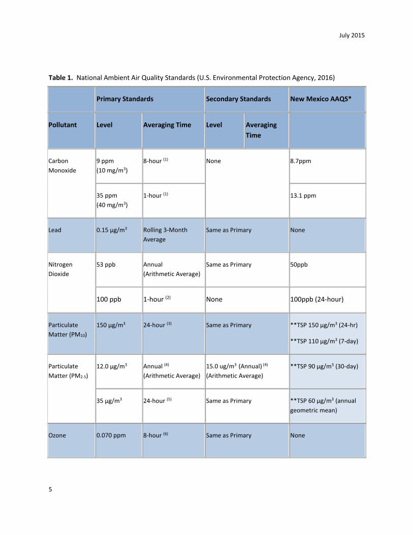
(NAAQS) for each criteria pollutant. Table 1 shows the current NAAQS for each pollutant. Regulation
and enforcement of the NAAQS has been delegated to the states by the EPA. New Mexico Ambient Air
Quality Standards (NMAAQS) are also shown. Oklahoma, Kansas and Texas do not have state standards
for criteria pollutants that differ from the NAAQS.
July 2015
5
Table 1. National Ambient Air Quality Standards (U.S. Environmental Protection Agency, 2016)
Primary Standards Secondary Standards New Mexico AAQS*
Pollutant Level Averaging Time Level Averaging
Time
Carbon
Monoxide
9 ppm
(10 mg/m3)
8-hour (1) None 8.7ppm
35 ppm
(40 mg/m3)
1-hour (1) 13.1 ppm
Lead 0.15 µg/m3 Rolling 3-Month
Average
Same as Primary None
Nitrogen
Dioxide
53 ppb Annual
(Arithmetic Average)
Same as Primary 50ppb
100 ppb 1-hour (2) None 100ppb (24-hour)
Particulate
Matter (PM10)
150 µg/m3 24-hour (3) Same as Primary **TSP 150 µg/m3 (24-hr)
**TSP 110 µg/m3 (7-day)
Particulate
Matter (PM2.5)
12.0 µg/m3 Annual (4)
(Arithmetic Average)
15.0 ug/m3 (Annual) (4)
(Arithmetic Average)
**TSP 90 µg/m3 (30-day)
35 µg/m3 24-hour (5) Same as Primary **TSP 60 µg/m3 (annual
geometric mean)
Ozone 0.070 ppm
8-hour (6) Same as Primary None
July 2015
6
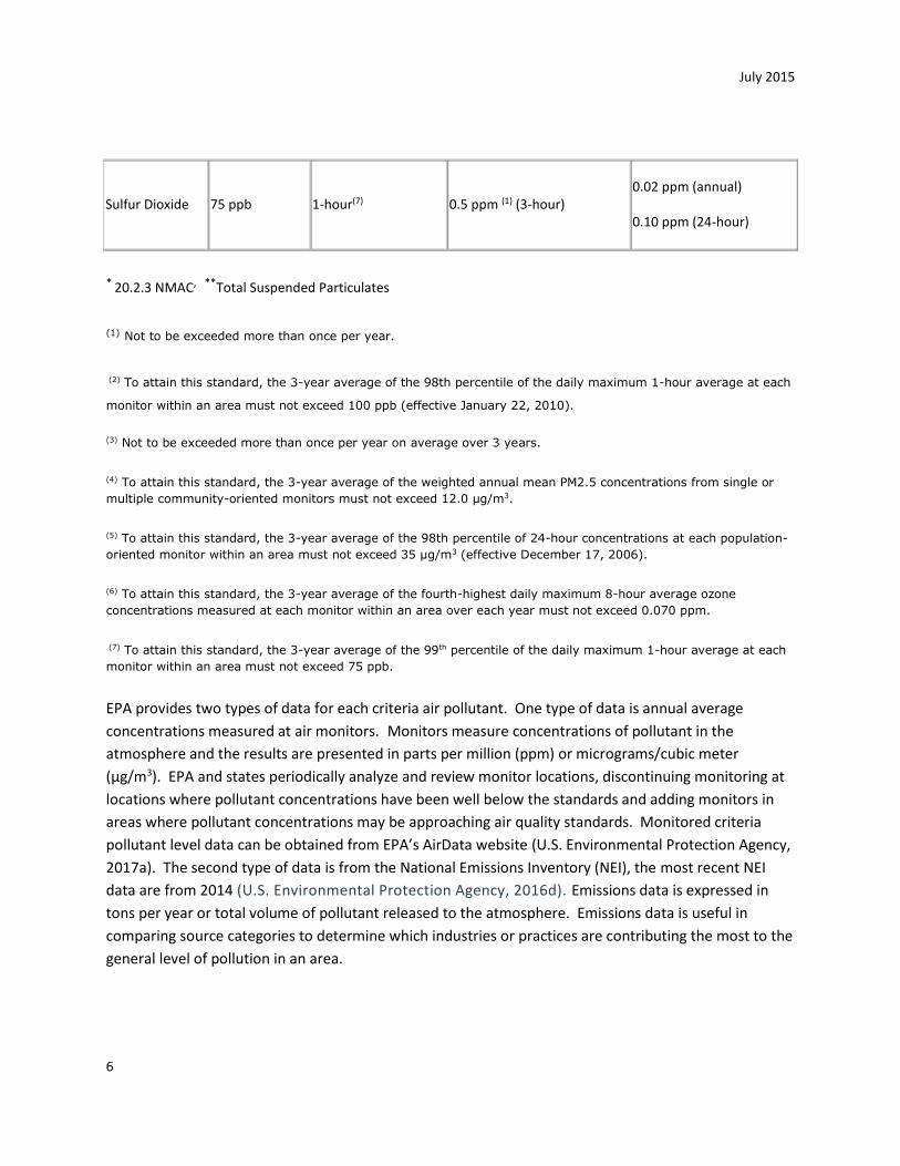
Sulfur Dioxide 75 ppb 1-hour(7) 0.5 ppm (1) (3-hour) 0.02 ppm (annual)
0.10 ppm (24-hour)
* 20.2.3 NMAC, **Total Suspended Particulates
(1) Not to be exceeded more than once per year.
(2) To attain this standard, the 3-year average of the 98th percentile of the daily maximum 1-hour average at each
monitor within an area must not exceed 100 ppb (effective January 22, 2010).
(3) Not to be exceeded more than once per year on average over 3 years.
(4) To attain this standard, the 3-year average of the weighted annual mean PM2.5 concentrations from single or
multiple community-oriented monitors must not exceed 12.0 µg/m3.
(5) To attain this standard, the 3-year average of the 98th percentile of 24-hour concentrations at each population-
oriented monitor within an area must not exceed 35 µg/m3 (effective December 17, 2006).
(6) To attain this standard, the 3-year average of the fourth-highest daily maximum 8-hour average ozone
concentrations measured at each monitor within an area over each year must not exceed 0.070 ppm.
(7) To attain this standard, the 3-year average of the 99th percentile of the daily maximum 1-hour average at each
monitor within an area must not exceed 75 ppb.
EPA provides two types of data for each criteria air pollutant. One type of data is annual average
concentrations measured at air monitors. Monitors measure concentrations of pollutant in the
atmosphere and the results are presented in parts per million (ppm) or micrograms/cubic meter
(μg/m3). EPA and states periodically analyze and review monitor locations, discontinuing monitoring at
locations where pollutant concentrations have been well below the standards and adding monitors in
areas where pollutant concentrations may be approaching air quality standards. Monitored criteria
pollutant level data can be obtained from EPA’s AirData website (U.S. Environmental Protection Agency,
2017a). The second type of data is from the National Emissions Inventory (NEI), the most recent NEI
data are from 2014 (U.S. Environmental Protection Agency, 2016d). Emissions data is expressed in
tons per year or total volume of pollutant released to the atmosphere. Emissions data is useful in
comparing source categories to determine which industries or practices are contributing the most to the
general level of pollution in an area.
July 2015
7
The NEI data present the emissions of each criteria pollutant by county for major source sectors.
National emissions trends are reported in the 2014 NEI Report (U.S. Environmental Protection Agency,
2017b). Details of the sectors mentioned in the report are:
(1) Electricity generation is fuel combustion from electric utilities;
(2) Fossil fuel combustion is fuel combustion from industrial boilers, internal combustion engines, and
commercial/institutional or residential use;
(3) Industrial processes include manufacturing of chemicals, metals, and electronics, storage and transfer
operations, pulp and paper production, cement manufacturing, petroleum refineries, and oil and gas
production;
(4) On-road vehicles category includes both gasoline- and diesel-powered vehicles for on-road use;
(5) Non-road equipment includes gasoline- and diesel-powered equipment for non-road use, as well as
planes, trains, and ships;
(6) Road dust includes dust from both paved and unpaved roads. Presentation of emissions data by source
sector provides a better understanding of the activities that contribute to criteria pollutant emissions.
NEI data for New Mexico, Kansas, Oklahoma and Texas can be found in Appendix A.
OZONE (O3)
Ground level ozone is not emitted directly into the air, but is created by chemical reactions between NOx
(oxides of nitrogen) and volatile organic compounds (VOC) in the presence of sunlight. Emissions from
industrial facilities and electric utilities, motor vehicle exhaust, gasoline vapors, and chemical solvents
are some of the major sources of NOx and VOC (U.S. Environmental Protection Agency, 2014a). VOCs
refer to “volatile” organic chemical compounds which participate in atmospheric photochemical
reactions to form secondary pollutants such as ozone which can affect the environment and human
health. VOCs are emitted from a variety of sources, such as refineries, oil and gas production equipment,
industrial processes, automobiles, consumer products and natural (or biogenic) sources, such as trees
and plants. While ozone and NO2 are criteria air pollutants, VOCs are not.
Nationally, ozone concentrations at urban and rural sites have decreased 22% from 1990 to 2015.
Weather conditions have a significant role in the formation of ozone. Ozone is most readily formed on
warm summer days when there is stagnation. Because of this role that weather plays in ozone
production, EPA uses a model to account for weather-related variability of ozone concentrations and
provide a more accurate assessment of the underlying trend in ozone precursor emissions. Removing
the effects of weather, national ozone concentrations in rural areas have decreased approximately 11%
from 2000 to 2015. In Carlsbad, NM, removing the effects of weather, ozone concentrations increased
July 2015
8
8% between 2000 and 2012, while ozone concentrations in Farmington, NM decreased 6% from 2000 to
2012. Ozone concentrations in Tulsa, Oklahoma decreased 23% from 2000 to 2015 and in Oklahoma
City decreased 18% from 2000 to 2015.Removing the effects of weather, ozone concentrations in Kansas
were the same in 2012 as in 2000. In Texas, ozone concentrations decreased substantially removing the
effects of weather, especially in large urban areas. Houston, Longview and Dallas ozone concentrations
decreased from 11-27% between 2000 and 2012, while concentrations in Austin and El Paso decreased
by 2-3%. San Antonio’s ozone concentrations increased 5% between 2000 and 2015, removing the
effects of weather (U.S. Environmental Protection Agency, 2016a).
VOCs are emitted during well drilling and operations as exhaust from internal combustion engines.
VOCs may be emitted from hydraulically fractured oil and gas wells during the fracturing and re-
fracturing of the wells. In the hydraulic fracturing process, a mixture of water, chemicals and proppant
is pumped into a well at extremely high pressures to fracture rock and allow oil and gas to flow from the
geological formation. During one stage of well completion, fracturing fluids, water and reservoir gas
come to the surface at high velocity and volume (flowback). This flowback mixture contains VOCs,
methane, benzene, ethylbenzene and n-hexane; some or all of the flowback mixture may be vented,
flared or captured. The typical flowback process lasts from 3 to 10 days, so there is potential for
significant VOC emissions from this stage of the well completion process. Most new oil and gas wells
drilled today use the hydraulic fracturing process. VOCs are also a component of natural gas and may be
emitted from equipment leaks, valves, pipes and pneumatic devices. NOx emissions are discussed
below under NO2.
An emissions inventory conducted for the Carlsbad Field Office for calendar year 2007 and including
Chaves, Lea, and Eddy counties (Applied Enviro Solutions, 2011) shows that VOC emissions from
biogenic (natural) sources are far greater than those from anthropogenic (human) sources and account
for 91% of VOCs inventoried. Point source emissions (which might include such industrial sources as
power plants, gas plants and oil refineries) account for 40% of anthropogenic VOC emissions in the area,
solvent use accounts for 15%, and fire (including wildland, structure, and open burning) accounts for 8%.
Oil and gas area sources produce only 1.4% of VOCs in the area while pipeline transport of oil and gas
accounts for 1.7%.
An emissions inventory conducted for the Four Corners region for calendar year 2005, including counties
in northwestern New Mexico, southwestern Colorado, southeastern Utah and northeastern Arizona,
estimates VOC emissions from biogenic sources account for 55% of total VOCs (Environ, 2009). In this
study, biogenic VOC emissions were calculated not measured. Oil and gas area and point sources
accounted for 28% of VOCs inventoried.
The 2014 NEI for the entire state of New Mexico estimates VOC emissions from biogenic sources
account for 82% of total VOCs in the state. VOCs from fire account for 2% and industrial processes
account for 12% of total VOCs. According to the 2014 NEI, Texas biogenic emissions account for 72% of

July 2015
9
total VOC emissions, while industrial processes account for 17% of VOC emissions. VOC emissions from
fire account for 2% of Texas VOC emissions, mobile sources account for 3% of total VOC emissions, and
solvents account for 4% of total VOC emissions. In Oklahoma, biogenic emissions are estimated to be
69% of total VOC emissions, industrial processes account for 14%, fire accounts for 7% of total VOC
emissions, and mobile sources account for 4% of total VOC emissions. In Kansas, biogenics account for
64% of total VOC emissions, fire accounts for 9% of VOC emissions, industrial processes account for 14%
of VOC emissions, mobile sources account for 5% of VOC emissions, and solvents account for 6% of VOC
emissions (U.S. Environmental Protection Agency, 2016d).
The current NAAQS for ozone is the three-year average of the annual fourth-highest daily maximum 8-
hour average ozone concentration, which for simplicity is sometimes referred to as the “design value.”
Between 1997 and 2008, the NAAQS for ozone was 0.08 ppm. To attain this standard, the design value
for ozone at any monitor in the U.S. could not exceed 0.084 ppm. In 2008, the NAAQS for ozone was
lowered to 0.075 ppm. In 2015, the NAAQS for ozone was lowered to 0.070 ppm.
In 2009, a photochemical modeling analysis was completed for the Four Corners Air Quality Task Force
(FCAQTF). Potential ozone impacts and the usefulness of certain mitigation measures were analyzed.
This modeling showed that the Four Corners region would continue to meet the current ozone standard
in 2018 with continued oil and gas development and population growth. The analysis showed that
emissions reductions would be required for both power plants and oil and gas sources in order to
achieve measurable reductions in ozone concentrations. The best achievable ozone reductions from the
modeling scenarios implementing control measures to reduce emissions were on the order of 5 ppb
(Environ, 2009).
The modeling analysis completed for FCAQTF also used source apportionment modeling, which
indicated that, in general, transport from outside the region and naturally occurring VOCs from
vegetation were large contributors to 2005 ozone levels. However it was also shown that on days with
high ozone concentrations, oil and gas sources and electricity generation units (EGUs) both contributed
significantly to the total modeled ozone concentrations.
In 2013, the Western Regional Air Partnership (WRAP) completed a regional technical analysis for ozone
(WestJump) that includes information about ozone impacts and sources that contribute to the
formation of ozone for calendar year 2008. The analysis demonstrated that the largest contributor to
ozone concentrations in the western U.S. was international transport and stratospheric ozone. State-to-
state ozone transport was important, as well. For example, New Mexico sources significantly contribute
to elevated ozone concentrations in Texas, Arizona and Colorado. Texas is a significant contributor to
elevated ozone in Oklahoma, Louisiana, New Mexico, Missouri and Arizona. Kansas sources significantly
contribute to elevated ozone in Missouri and Texas, while Oklahoma sources significantly contribute to
elevated ozone in Missouri, Texas and New Mexico (ENVIRON International Corporation, Alpine
Geophysics, LLC and University of North Carolina, 2013).

July 2015
10
NITROGEN DIOXIDE (NO2)
NO2 is both a criteria pollutant and an indicator for the NOx family of nitrogen oxide compounds that are
ground-level ozone precursors. The nitrogen oxide family of compounds includes nitric oxide (NO),
nitrogen dioxide (NO2), nitrous acid (HN02), and nitric acid (HNO3). The primary sources of NOx nationally
are motor vehicles and fuel combustion. The excess air required for complete combustion of fuels in
these processes introduces atmospheric nitrogen into the combustion reactions at high temperatures
and produces nitrogen oxides. NO2 has been shown to cause adverse respiratory impacts in both healthy
people and those with asthma, and is also an important contributor to the formation of ground-level
ozone (U.S. Environmental Protection Agency, 2014b).
Nationally, NO2 concentrations have decreased substantially (47% reduction) from 2000 to 2015. In the
southwest (Arizona, New Mexico, Colorado and Utah), NO2 concentrations have decreased 32%
between 2000 and 2015; in the south (Texas, Oklahoma, Kansas, Arkansas, Louisiana and Mississippi),
NO2 concentrations have decreased 27% between 2000 and 2015. EPA expects NO2 concentrations will
continue to decrease because of a number of motor vehicle standards that are taking effect (U.S.
Environmental Protection Agency, 2016b).
NOx emissions in the Carlsbad area are largely anthropogenic (88%). Of the total human-caused NOx
emissions, industrial point sources account for 84%, on-road mobile sources account for 7%, oil and gas
area sources account for 5%, non-road mobile sources account for 2%, and residential heating with
natural gas and propane account for 1% (Applied Enviro Solutions, 2011).
The top three sources of NOx emissions in the Farmington area in 2005 were electricity generation
(72,668 tons; 33%), oil and gas (68,830 tons; 31%) and on-road mobile sources (39,340 tons; 18%)
(Environ, 2009).
The 2014 National Emissions Inventory data for the Farmington area (San Juan County), indicates that
fuel combustion accounts for 56% of total NOx emissions, industrial sources account for 34% of total
NOx emissions, and mobile sources account for 9% of total NOx emissions in the area (U.S.
Environmental Protection Agency, 2016d).
The 2014 National Emissions Inventory data for the state of New Mexico indicate mobile sources
account for 44%, fuel combustion accounts for 22%, industrial processes account for 19%, biogenics
account for 13% and fire accounts for less than 1% of total NOx emissions in the state. For Texas, the
2014 National Emissions Inventory data indicate mobile sources account for 47%, fuel combustion
accounts for 19%, industrial processes account for 25%, biogenics account for 8% and fire accounts for
less than 1% of total NOx emissions in the state. In Oklahoma, mobile sources account for 35%, fuel
combustion accounts for 29%, industrial processes account for 24%, biogenics account for 10% and fire
accounts for 2% of total Oklahoma NOx emissions. In Kansas, mobile sources account for 41%, fuel
July 2015
11
combustion accounts for 20%, industrial processes account for 20%, biogenics account for 16% and fire
accounts for 3% of total Kansas NOx emissions (U.S. Environmental Protection Agency, 2016d).
CARBON MONOXIDE (CO)
Carbon monoxide is produced from the incomplete burning of carbon-containing compounds such as
fossil fuels; it forms when there is not enough oxygen to produce carbon dioxide (CO2). Nationally, 86%
of CO emissions come from transportation sources. CO is associated with negative health effects to
human cardiovascular, central nervous, and respiratory systems (U.S. Environmental Protection Agency,
2014c). There are currently no non- attainment areas for CO in the United States (U.S. Environmental
Protection Agency, 2016e).
Nationally, CO concentrations have decreased 77% from 2000 to 2015. Monitored CO concentrations in
the “southwest” region (New Mexico, Arizona, Colorado and Utah) have decreased 60% between 2000
and 2015. Monitored CO concentrations in the “south” region (Texas, Oklahoma, Kansas, Arkansas,
Louisiana and Mississippi) have decreased 64% between 2000 and 2013 (U.S. Environmental Protection
Agency, 2016c).
The 2007 emissions inventory for Chaves, Eddy, and Lea Counties shows that anthropogenic sources
account for 65% of CO emissions and biogenic sources 35%. Of the anthropogenic emissions 47% are
from on road mobile sources, 24% from industrial point sources, 14% from non-road mobile sources, 9%
from fire, and 2% each from oil and gas area sources and waste disposal burning (Applied Enviro
Solutions, 2011).
For San Juan County, New Mexico (Farmington area), the 2014 National Emissions Inventory data
indicate fires contribute 32%, mobile sources contribute 18%, fuel combustion contributes 15%,
industrial processes contribute 21% and biogenics contribute 13% of total CO emissions in the county
(U.S. Environmental Protection Agency, 2016d).
For New Mexico, the 2014 National Emissions Inventory data indicate mobile sources account for 34%,
industrial processes account for 8%, fuel combustion accounts for 5%, fire accounts for 14% and
biogenics account for 37% of total state CO emissions. The 2014 National Emissions inventory data for
Texas indicate mobile sources account for 50%, fuel combust accounts for 6%, industrial processes
account for 5%, fire accounts for 14% and biogenics account for 21% of total Texas CO emissions. In
Oklahoma, mobile sources account for 38%, fuel combustion accounts for 6%, industrial processes
account for 7%, fire accounts for 36% and biogenics account for 11% of total CO emissions in the state.
In Kansas, mobile sources account for 38%, fuel combustion accounts for 6%, industrial processes
account for 9%, fire accounts for 33% and biogenics account for 13% of total CO emissions in the state
(U.S. Environmental Protection Agency, 2016d).

July 2015
12
PARTICULATE MATTER (PM)
Particulate matter, also known as particle pollution or PM, is a complex mixture of extremely small
particles and liquid droplets. PM is made up of a number of components, including acids (such as
nitrates and sulfates), organic chemicals, metals, and soil or dust particles. PM is measured and
regulated according to particle size. PM10 refers to all particles with a diameter of 10 microns or less.
PM2.5 is made up of particles with diameters of 2.5 microns or less. Smaller particles are associated with
more negative health effects, including respiratory and cardiovascular problems because they can
become more deeply embedded in the lungs (U.S. Environmental Protection Agency, 2013).
Nationally, PM2.5 concentrations have decreased 37% from 2000 to 2015. In that same time period,
PM10 concentrations decreased 36% nationally. In the Four Corners region (New Mexico, Arizona,
Colorado and Utah), PM2.5 concentrations have decreased 24% from 2000 to 2015, and PM10
concentrations have decreased 16% in the same time period. For the southern region encompassing
Texas, Oklahoma, Kansas, Arkansas, Louisiana and Mississippi, PM2.5 concentrations have decreased 31%
and PM10 concentrations have decreased 10% between 2000 and 2015 (U.S. Environmental Protection
Agency, 2016g) & (U.S. Environmental Protection Agency, 2016f).
A 2007 emissions inventory for Chaves, Eddy, and Lea Counties shows that the bulk of emission for both
PM10 and PM2.5 are from dust from unpaved roads (88 and 65% respectively). For PM10, the next
three highest categories are point sources at 2.8%, tilling and harvesting 2.6% and paved roads 2.4%. Oil
and gas area sources account for only 0.1% of PM10 emissions. For PM2.5, the next three highest
categories are point sources at 17%, fire at 4.3% and tilling and harvesting at 2.8%. Oil and gas area
sources account for 0.8% of PM2.5 emissions in this area (Applied Enviro Solutions, 2011).
For the Farmington area (San Juan County), the 2014 National Emissions Inventory data show that most
particulate matter emissions are from dust (PM2.5: 5,062 tons, 56%; PM10: 48,187 tons, 87%) (U.S.
Environmental Protection Agency, 2016d).
According to the 2014 National Emissions Inventory, for the entire state of New Mexico, dust accounts
for 68% and fire accounts for 12% of PM2.5 emissions statewide. For PM10, dust accounts for 91% and
fire accounts for 2% of emissions in New Mexico. For Texas, the 2014 National Emissions Inventory data
indicate that dust accounts for 45%, fire accounts for 13%, agriculture accounts for 18%, mobile sources
account for 6%, fuel combustion accounts for 6% and industrial processes accounts for 6% of statewide
PM2.5 emissions. Dust accounts for 75%, agriculture accounts for 16% and fire accounts for 3% of Texas
PM10 emissions. In Oklahoma, fire accounts for 27%, dust accounts for 37%, agriculture accounts for
21%, fuel combustion accounts for 5%, industrial processes account for 4% and mobile sources account
for 3% of Oklahoma PM2.5 emissions. Dust accounts for 69%, agriculture accounts for 21% and fire
accounts for 6% of Oklahoma PM10 emissions. In Kansas, dust accounts for 25%, agriculture accounts for
41%, fire accounts for 21%, mobile sources account for 4%, industrial sources account for 3% and fuel

July 2015
13
combustion accounts for 4% of Kansas PM2.5 emissions. Agriculture accounts for 42%, dust accounts for
49% and fire accounts for 6% of Kansas PM10 emissions (U.S. Environmental Protection Agency, 2016d).
The WestJump analysis also provides information about PM2.5 impacts and contributing sources for
calendar year 2008. Interstate transport is significant for PM2.5. New Mexico significantly contributes to
annual PM2.5 exceedances in Arizona; Texas significantly contributes to exceedances in Arkansas,
Missouri, Mississippi, Illinois and Alabama; Oklahoma significantly contributes to exceedances in
Arkansas and Missouri, and Kansas significantly contributes to exceedances in Iowa, Missouri, Illinois,
Arkansas and Wisconsin. For the 24-hour PM2.5 standard, New Mexico significantly contributes to
exceedances in California, Texas and Oklahoma significantly contribute to exceedances in Iowa, and
Kansas significantly contributes to exceedances in Iowa and Wisconsin (ENVIRON International
Corporation, Alpine Geophysics, LLC and University of North Carolina, 2013).
SULFUR DIOXIDE (SO2)
Sulfur dioxide (SO2) is one of a group of highly reactive gases known as “oxides of sulfur,” commonly
referred to as SOx. The largest sources of SO2 emissions nationwide are from fossil fuel combustion at
power plants (73%) and other industrial facilities (20%). Smaller sources of SO2 emissions include
industrial processes, such as extracting metal from ore, and the burning of high sulfur-containing fuels
by locomotives, large ships, and non-road equipment. SO2 is linked with a number of adverse effects on
the respiratory system (U.S. Environmental Protection Agency, 2015a).
Nationally, SO2 concentrations have decreased 81% from 2000 to 2015, but substantial decreases (76%
reduction) have occurred since 1980 due to implementation of federal rules requiring reductions in SO2
emissions from power plants and other large sources of SO2. In the Four Corners region, SO2
concentrations decreased 24% between 2000 and 2015. In the southern region of Texas, Oklahoma,
Kansas, Arkansas, Louisiana and Mississippi, SO2 concentrations decreased 76% between 2000 and 2015
(U.S. Environmental Protection Agency, 2016i).
The Carlsbad area, the 2007 emissions inventory does not differentiate SO2 from SOx but it can be
assumed that the percentage of emissions by category is similar. In this region, oil and gas area sources
account for 74% of all SOx emissions with most of the remainder, 25% accounted for by industrial point
sources (Applied Enviro Solutions, 2011).
In the Farmington area nearly all SO2 emissions come from fuel combustion (5,038 tons; 93%), while 4%
of SO2 emissions come from fires and 3% from industrial sources, according to the 2014 National
Emissions Inventory (U.S. Environmental Protection Agency, 2016d).
The 2014 National Emissions Inventory data indicate industrial sources account for 46%, fuel
combustion accounts for 44%, fires account for 5%, and mobile sources account for 4%, of New Mexico

July 2015
14
SO2 emissions. Fuel combustion accounts for 78% and industrial processes account for 20% of Texas SO2
emissions. Fuel combustion accounts for 73%, industrial processes account for 22% and fire accounts
for 4% of Oklahoma SO2 emissions. Fuel combustion accounts for 79%, fire accounts for 8% and
industrial processes account for 11% of Kansas SO2 emissions (U.S. Environmental Protection Agency,
2016d).
LEAD
With the elimination of lead from gasoline and regulation of industrial sources, levels of lead in the
atmosphere decreased 94% nationwide between 1980 and 1999. Lead concentrations decreased 60%
nationally between 2000 and 2013. While still regulated as a criteria pollutant, the major sources of
lead pollution are lead smelters and leaded aviation gasoline. In 2014, EPA proposed to retain the
NAAQS for lead without revision (U.S. Environmental Protection Agency, 2014d).
According to the 2014 National Emissions Inventory, aircraft account for 77% of the lead emissions in
New Mexico. In Texas, 79% of the lead emissions are from aircraft. In Oklahoma, 47% of lead emissions
are from aircraft and 29% are from waste disposal. In Kansas, 81% of lead emissions are from aircraft
(U.S. Environmental Protection Agency, 2016d).
HAZARDOUS AIR POLLUTANTS
The U.S. Congress amended the Federal Clean Air Act in 1990 to address a large number of air pollutants
that are known to cause or may reasonably be anticipated to cause adverse effects to human health or
adverse environmental effects. Congress initially identified 188 specific pollutants and chemical groups
as hazardous air pollutants (HAPs) and has modified the list over time.
The Clean Air Act requires control measures for hazardous air pollutants. National emissions standards
for hazardous air pollutants (NESHAPs) are issued by EPA to limit the release of specified HAPs from
specific industrial sectors. These standards are technology based, meaning that they represent the
maximum achievable control technology that is economically feasible for an industrial sector.
The CAA defines a major source for HAPs to be one emitting 10 tons per year of any single HAP or 25
tons per year of any combination of HAPs. Under state regulations, a construction or operating permit
may be required for any major source though some exceptions apply. In New Mexico, these regulations
are 20.2.70 and 20.2.73 NMAC, in Texas the regulation is 30 TAC 122, in Kansas, the regulation is K.A.R.
28-19-500 and in Oklahoma, the regulation is OAR 252-100-7. Within its definition of a major source in
the above referenced regulations the state of New Mexico includes the following language:
…hazardous emissions from any oil or gas exploration or production well (with its
associated equipment) and hazardous emissions from any pipeline compressor or pump

July 2015
15
station shall not be aggregated with hazardous emissions from other similar units,
whether or not such units are in a contiguous area or under common control, to determine
whether such units or stations are major sources…
In other words, in determining a major source, each oil and gas exploration and production well must be
considered singularly. Kansas, Texas and Oklahoma regulations include similar language.
NESHAPs for Oil and Natural Gas Production and Natural Gas Transmission and Storage were published
by EPA on June 17, 1999. These NESHAPs were directed toward major sources and intended to control
benzene, toluene, ethyl benzene, mixed xylenes and n-hexane. An additional NESHAP for Oil and
Natural Gas Production Facilities directed toward area sources was published on January 3, 2007 and
specifically addresses benzene emissions from triethylene glycol dehydrations units. The EPA issued a
final rule revising the NESHAP effective October 15, 2012. The final rule includes revisions to the
existing leak detection and repair requirements and established emission limits reflecting maximum
achievable control technology for currently uncontrolled emission sources in oil and gas production and
natural gas transmission and storage (Fed. Reg. 77(159): 49490-49600, August 16, 2012).
The state of New Mexico incorporates federal NESHAPs for pollutants through updates to 20.2.78
NMAC, which adopts 40 CFR Part 61, and federal NESHAPs for source categories through updates to
20.2.82 NMAC, which adopts 40 CFR Part 63. Similarly, Texas incorporates federal NESHAPs for both 40
CFR 61 and 40 CFR 63 through updates to 30 TAC 113. Kansas incorporates federal NESHAPs by
adopting 40 CFR 61 through updates to K.A.R. 28-19-735 and incorporates NESHAP source categories at
40 CFR 63 through updates to K.A.R. 28-19-750. Oklahoma incorporates both 40 CFR 61 and 40 CFR 63
through O.A.R. 252-100-41-2 and Appendix Q.
In March 2011, EPA published the fourth in a series of National Scale Air Toxics Assessments (NATA).
Based on 2005 data including the National Emissions Inventory, the NATA is intended to be a tool to
help focus emissions reduction strategies (U.S. Environmental Protection Agency, 2013a). Computer
models are used to develop estimates of risk of cancer or other health impacts from air toxic emissions.
NATA presents risk hazard indexes for cancer, neurological and respiratory problems for each county
and census tract. Because techniques have changed over the years, each NATA is not comparable to
those previously issued. EPA also cautions that because data availability varies from state to state, the
results are not necessarily comparable from one geographic area to another. NATA data for New
Mexico, Kansas, Oklahoma, and Texas can be found in Appendix B.
HYDROGEN SULFIDE (H2S)
H2S is a colorless flammable gas with a rotten egg smell which is a naturally occurring byproduct of oil
and gas development in some areas, including the New Mexico portion of the Permian Basin. Hydrogen
sulfide is both an irritant and a chemical asphyxiant with effects on both oxygen utilization and the
July 2015
16
central nervous system. Its health effects can vary depending on the level and duration of exposure.
Effects may range from eye, nose and throat irritation to dizziness, headaches and nausea. High
concentrations can cause shock, convulsions, inability to breathe, extremely rapid unconsciousness,
coma and death. Effects can occur within a few breaths, and possibly a single breath.
H2S was originally included in the list of Toxic Air Pollutants defined by Congress in the 1990
amendments to the Clean Air Act. It was later determined that H2S was included through a clerical error
and it was removed by Congress from the list. H2S was addressed under the accidental release
provisions of the Clean Air Act. Congress also tasked EPA with assessing the hazards to public health and
the environment from H2S emissions associated with oil and gas extraction. That report was published
in October 1993 (U.S. Environmental Protection Agency, 1993).
EPA found that while there was a potential for human and environmental exposure from routine
emissions of H2S from oil and gas wells, there was insufficient evidence to suggest that these exposures
were a significant threat. H2S is present in some oil and gas production zones. Flaring is used to reduce
the H2S emissions and the CFO has developed a series of standard conditions of approval for high H2S
areas in order to mitigate the risk of H2S exposure.
Hydrogen Sulfide was added to the Emergency Planning and Community Right-to-Know Act list of toxic
chemicals in 1993. In 1994, EPA issued an administrative stay of reporting requirements for H2S while
further analysis was conducted. The administrative stay was lifted recently, and TRI reporting due in
July 2013 for calendar year 2012 emissions required reporting of H2S.
While there are no national ambient air quality standards for H2S, a number of states, especially those
with significant oil and gas production, have set standards at the state level. Table 2 summarizes these
standards for states under BLM New Mexico State Office jurisdiction.

July 2015
17
Table 2. State Ambient Air Quality Standards for H2S (Skrtic, 2006)
State Standard Averaging time Remarks
Kansas None
Oklahoma 200 ppb*
(0.2 ppm) 24 hr
New Mexico
0.010 ppm**
(10 ppb) 1 hr
Statewide except Pecos-Permian Basin Intrastate Air
Quality Control Region***
0.100 ppm
(100 ppb) ½ hr
Pecos-Permian Basin Intrastate Air Quality Control
Region
0.030ppm
(30 ppb) ½ hr
Within municipal boundaries and within five miles of
municipalities with population >20,000 in Pecos-
Permian Basin AQ Control Region
Texas 0.08ppm
(80 ppb) ½ hr
If downwind concentration affects a property used
for residential business or commercial purposes
0.12 ppm
(120 ppb) ½ hr
If downwind concentration affects only property not
normally occupied by people
*parts per billion **parts per million *** The Pecos-Permian Basin Intrastate Air Quality Control Region is composed of Quay, Curry, De Baca,
Roosevelt, Chaves, Lea, and Eddy Counties in New Mexico.
The New Mexico Environment Department (NMED) has no routine monitors for H2S. However, a one-
time study done in 2002 (Skrtic, 2006) sheds some light on the levels which can be expected near oil and
gas facilities. These readings are averaged over 3 minute periods so are not comparable with the
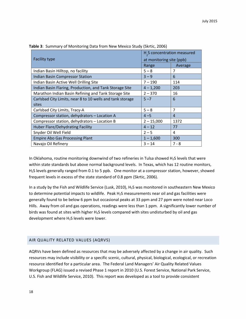
standard which has longer averaging periods. The monitoring data is presented in Table 3.
July 2015
18
Table 3: Summary of Monitoring Data from New Mexico Study (Skrtic, 2006)
Facility type
H2S concentration measured
at monitoring site (ppb)
Range Average
Indian Basin Hilltop, no facility 5 – 8 7
Indian Basin Compressor Station 3 – 9 6
Indian Basin Active Well Drilling Site 7 – 190 114
Indian Basin Flaring, Production, and Tank Storage Site 4 – 1,200 203
Marathon Indian Basin Refining and Tank Storage Site 2 – 370 16
Carlsbad City Limits, near 8 to 10 wells and tank storage sites
5 –7 6
Carlsbad City Limits, Tracy-A 5 – 8 7
Compressor station, dehydrators – Location A 4 –5 4
Compressor station, dehydrators – Location B 2 – 15,000 1372
Huber Flare/Dehydrating Facility 4 – 12 77
Snyder Oil Well Field 2 – 5 4
Empire Abo Gas Processing Plant 1 – 1,600 300
Navajo Oil Refinery 3 – 14 7 - 8
In Oklahoma, routine monitoring downwind of two refineries in Tulsa showed H2S levels that were
within state standards but above normal background levels. In Texas, which has 12 routine monitors,
H2S levels generally ranged from 0.1 to 5 ppb. One monitor at a compressor station, however, showed
frequent levels in excess of the state standard of 0.8 ppm (Skrtic, 2006).
In a study by the Fish and Wildlife Service (Lusk, 2010), H2S was monitored in southeastern New Mexico
to determine potential impacts to wildlife. Peak H2S measurements near oil and gas facilities were
generally found to be below 6 ppm but occasional peaks at 33 ppm and 27 ppm were noted near Loco
Hills. Away from oil and gas operations, readings were less than 1 ppm. A significantly lower number of
birds was found at sites with higher H2S levels compared with sites undisturbed by oil and gas
development where H2S levels were lower.
AIR QUALITY RELATED VALUES (AQRVS)
AQRVs have been defined as resources that may be adversely affected by a change in air quality. Such
resources may include visibility or a specific scenic, cultural, physical, biological, ecological, or recreation
resource identified for a particular area. The Federal Land Managers’ Air Quality Related Values
Workgroup (FLAG) issued a revised Phase 1 report in 2010 (U.S. Forest Service, National Park Service,
U.S. Fish and Wildlife Service, 2010). This report was developed as a tool to provide consistent

July 2015
19
approaches to the analysis of the effects of air pollution on AQRVs. The FLAG report focuses on three
areas of potential impact: visibility, aquatic and terrestrial effects of wet and dry pollutant deposition,
and terrestrial effects of ozone. This report is structured to address these same three areas of potential
impact.
VISIBILITY
Visibility is of greatest concern in Class I areas which are afforded the highest level of air quality
protection by the Clean Air Act. Visibility impairment is a result of regional haze which is caused by the
accumulation of pollutants from multiple sources in a region. Emissions from industrial and natural
sources may undergo chemical changes in the atmosphere to form particles of a size which scatter or
absorb light and result in reductions in visibility.
In 1985, the EPA initiated a network of monitoring stations to measure impacts to visibility in Class I
Wilderness Areas. These monitors are known as the Interagency Monitoring for the Protection of Visual
Environments (IMPROVE) monitors and exist in some, but not all, Class I wilderness areas. Table 4
shows the Class I areas in the BLM New Mexico State Office area of responsibility and whether they have
an IMPROVE monitor and, if not, which monitor is considered representative for that area. There are no
Class I areas in Kansas.
Table 4. Class I areas and IMPROVE monitors
State Class I Area Agency IMPROVE
New Mexico Bandelier National Park Service Yes
Bosque del Apache Fish and Wildlife Yes
Carlsbad Caverns National Park Service Guadalupe Mtns
Gila Forest Service Yes
Pecos Forest Service Wheeler Peak
Salt Creek Fish and Wildlife Yes
San Pedro Parks Forest Service Yes
Wheeler Peak Forest Service Yes
White Mountain Forest Service Yes
Texas Big Bend National Park Service Yes
Guadalupe Mtns National Park Service Yes
Oklahoma Wichita Mountains Fish and Wildlife Yes
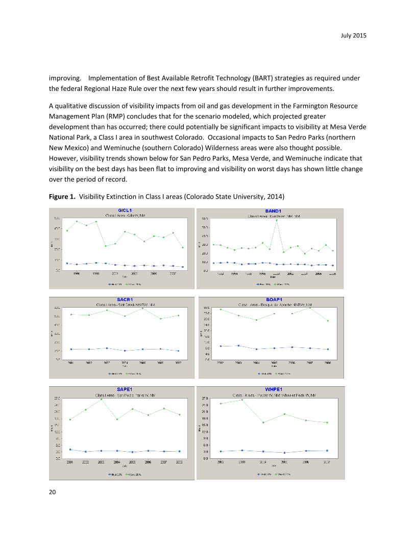
Figure 1 shows visibility extinction trends for each of the IMPROVE monitors in the BLM New Mexico
State Office area of responsibility. The top line on each graph is for the 20% worst days and the bottom
line is for the 20% best days. Note that peaks such as that seen for Bandelier National Monument in
2000 may be accounted for by the occurrence of large wildfires. A downward sloping line means less
reduction of visibility and therefore an improvement. In most cases visibility trends have been flat or
July 2015
20
improving. Implementation of Best Available Retrofit Technology (BART) strategies as required under
the federal Regional Haze Rule over the next few years should result in further improvements.
A qualitative discussion of visibility impacts from oil and gas development in the Farmington Resource
Management Plan (RMP) concludes that for the scenario modeled, which projected greater
development than has occurred; there could potentially be significant impacts to visibility at Mesa Verde
National Park, a Class I area in southwest Colorado. Occasional impacts to San Pedro Parks (northern
New Mexico) and Weminuche (southern Colorado) Wilderness areas were also thought possible.
However, visibility trends shown below for San Pedro Parks, Mesa Verde, and Weminuche indicate that
visibility on the best days has been flat to improving and visibility on worst days has shown little change
over the period of record.
Figure 1. Visibility Extinction in Class I areas (Colorado State University, 2014)

July 2015
21
Trend lines for Class I areas affected by sources in Northwestern New Mexico (Figure 2) are similar to
trend lines for Class I areas in New Mexico. While visibility on worst days at Guadalupe Mountains
National Park may have diminished, a careful analysis of fire activity in the area would be necessary in
order to draw conclusions about the cause of some peaks in recent years (Colorado State University,
2014).
A recent study of Air Pollutant Emissions and Cumulative Air Impacts done for the Carlsbad Field Office
indicates that pollutants contributing to reductions in visibility are largely coming from outside the
region (Applied Enviro Solutions, 2011).

July 2015
22
Figure 2. Visibility trends at Class I areas affected by sources in Northwestern New Mexico (Colorado State University, 2014)
The WestJump analysis (ENVIRON International Corporation, Alpine Geophysics, LLC and University of
North Carolina, 2013) provides a wealth of information about visibility impairment at Class I areas and the
source categories and states that contribute to impairment at each Class I area. There are two pie charts
for each of IMPROVE sites in New Mexico, Texas, Oklahoma and Kansas. These pie charts are presented
in Appendix F. The first pie chart displays the contributions of the 17 western states by source category
and species to visibility impairment for the IMPROVE site for the average of the worst 20% days. The
second pie chart displays contributions by the 17 western states to visibility impairment for the IMPROVE
site for the average of the worst 20% days. The pie chart data is from the CAMx 2006 36 km state-specific
PM source apportionment modeling. The source category codes in the pie charts are:
CON=controllable emissions (anthropogenic and Rx and Ag fires);
NAT=natural emissions (biogenic, lightning, sea salt and windblown dust);
WLF=wildfires.
The species codes in the pie charts are:
PMC=Crustal
PEC=elemental carbon
PNO3=nitrate
POM=organic PM
PSO4=sulfate
SSL=salt
SSR=Rayleigh
Soil=Soil
July 2015
23
WET AND DRY POLLUTANT DEPOSITION
Deposition of pollutants through precipitation can result in acidification of water and soil resources in
areas far removed from the source of the pollution, as well as causing harm to terrestrial and aquatic
species. Some pollutants can also damage vegetation through direct or dry deposition. In general, the
soils in New Mexico have a high acid neutralizing capacity and surface water is scarce, resulting in
minimal impacts in this area. Also, the Acid Rain Program has resulted in greatly reduced levels of the
most damaging pollutants. There are currently four wet deposition monitors in New Mexico including
Gila Cliff Dwellings, Mayhill, Bandelier National Monument, and Capulin Volcano National Monument.
In addition monitors near the border at Mesa Verde and Guadalupe Mountains National Parks may shed
some light on conditions in New Mexico. Data can be accessed through the National Atmospheric
Deposition Network (NADP) at http://nadp.sws.uiuc.edu/NTN/ntnData.aspx. Wet deposition data is also
available for monitoring sites in Kansas, Oklahoma, and Texas at this site.
The EPA has operated the Clean Air Status and Trends Network (CASTNET) since 1991 to provide data to
assess trends in air quality, deposition and ecological effects due to changes in air emissions. Sites are
located in areas where urban influences are minimal. There are currently no CASTNET observation sites
in New Mexico but there are three in Texas and one each in Oklahoma and Kansas. There is a CASTNET
site at Mesa Verde National Park in the Four Corners region. National maps of pollutant concentrations
can be found at http://www.epa.gov/castnet/javaweb/airconc.html. These maps show that New
Mexico and most of the western United States have much lower concentrations of all monitored
pollutants than the eastern states and southern California. Nitrates are somewhat elevated in eastern
Kansas and eastern Oklahoma but this is likely associated with agricultural activities rather than oil and
gas development. The maps also show that the trend over the past 20 years has been for decreases in
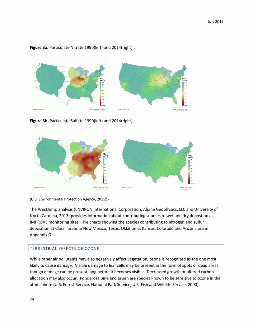
all pollutants in most areas of the country. As an example, Figure 3 shows particulate nitrate and sulfate
levels for 1990 and 2011. Maps of wet deposition data from NADP monitors are also available from the
National Atmospheric Deposition Program (National Atmospheric Deposition Program, 2014). Total dry
and wet sulfur deposition decreased by 63% from 1990 through 2012 in the eastern U.S. and decreased
by 39% from 1996 through 2012 in the west. Total nitrogen deposition decreased by 24% from 1990
through 2012 in the eastern U.S. and decreased by 20% in the western U.S. between 1996 through 2012;
however, total nitrogen deposition increased significantly in the eastern U.S. from 2010 to 2011. These
trends in deposition levels are discussed in depth in the CASTNET annual report (AMEC Environment and
Infrastructure, Inc., 2014).
July 2015
24
Figure 3a. Particulate Nitrate 1990(left) and 2014(right)
Figure 3b. Particulate Sulfate 1990(left) and 2014(right)
(U.S. Environmental Protection Agency, 2015b)
The WestJump analysis (ENVIRON International Corporation, Alpine Geophysics, LLC and University of
North Carolina, 2013) provides information about contributing sources to wet and dry depostion at
IMPROVE monitoring sites. Pie charts showing the species contributing to nitrogen and sulfur
deposition at Class I areas in New Mexico, Texas, Oklahoma, Kansas, Colorado and Arizona are in
Appendix G.
TERRESTRIAL EFFECTS OF OZONE
While other air pollutants may also negatively affect vegetation, ozone is recognized as the one most
likely to cause damage. Visible damage to leaf cells may be present in the form of spots or dead areas,
though damage can be present long before it becomes visible. Decreased growth or altered carbon
allocation may also occur. Ponderosa pine and aspen are species known to be sensitive to ozone in the
atmosphere (U.S. Forest Service, National Park Service, U.S. Fish and Wildlife Service, 2000).

July 2015
25
An index has been developed to express cumulative seasonal impacts to vegetation. This is known as
the W126 value. W126 is a cumulative metric that sums weighted hourly ozone concentrations during
daylight hours in the summer ozone season. Figure 4 shows national W126 values for 2012 (AMEC
Environment and Infrastructure, Inc., 2014). Higher W126 values were measured during 2012 in
California, at high terrain sites in the west and at eastern sites with high daily 8-hour ozone
concentrations. At high elevations, moderate ozone concentrations persist into the night due to lack of
nighttime dry deposition and lack of fresh nitric oxide, both of which typically react with ozone at night
to reduce ozone concentrations. The persistent, moderate ozone concentrations at high elevation sites
result in higher W126 levels, indicative of steady ozone exposure for vegetation. In 2012, W126 values
were higher than in 2011 because of higher ambient ozone concentrations measured in 2012.
Figure 4. W126 values for 2012 in ppm-hour (AMEC Environment and Infrastructure, Inc., 2014)
July 2015
26
CLIMATE, CLIMATE CHANGE & GREENHOUSE GASES
Climate is the composite of generally prevailing weather conditions of a particular region throughout the
year, averaged over a series of years. Climate averages for 1981-2010, known as the current normal as
defined by the World Meteorological Organization, are 30 year averages of temperature and
precipitation for the previous three decades and are included in Appendix C.
Climate change is a statistically-significant and long-term change in climate patterns. The terms climate
change and “global warming” are often used interchangeably, although they are not the same thing.
Climate change is any deviation from the average climate, whether warming or cooling, and can result
from both natural and human (anthropogenic) sources. Natural contributors to climate change include
fluctuations in solar radiation, volcanic eruptions, and plate tectonics. Global warming refers to the
apparent warming of climate observed since the early-twentieth century and is primarily attributed to
human activities such as fossil fuel combustion, industrial processes, and land use changes.
Climate change may reinforce (positive feedback) or reduce (negative feedback) an expected
temperature increase. A feedback is the process by which changing one quantity results in the
amplification or diminishment of another. An example of a positive feedback is the reduced albedo
(reflectivity) of land surfaces from the melting of snow and ice. A warming climate is also expected to
increase methane release from hydrates, thereby reinforcing the warming trend. There are also
feedbacks related to carbon, water, and geochemical cycles. The results of most climate feedbacks are
expected to amplify warming, but the exact magnitudes of these effects are difficult to quantify
(Intergovernmental Panel on Climate Change (IPCC), 2013).
The natural greenhouse effect is critical to the discussion of climate change. The greenhouse effect
refers to the process by which greenhouse gases (GHGs) in the atmosphere absorb heat energy radiated
by earth’s surface. Water vapor is the most abundant GHG, followed by carbon dioxide (CO2), methane
(CH4), nitrous oxide (N2O), and several trace gases. These GHGs trap heat that would otherwise be
radiated into space, causing earth’s atmosphere to warm and making temperatures suitable for life on
earth. Without the natural greenhouse effect, the average surface temperature of the earth would be
about zero degrees Fahrenheit. Water vapor is often excluded from the discussion of GHGs and climate
change since its atmospheric concentration is largely dependent upon temperature rather than being
emitted by specific sources.
Atmospheric concentrations of naturally-emitted GHGs have varied for millennia and earth’s climate
fluctuated accordingly. However, since the beginning of the industrial revolution around 1750, human
activities have significantly increased GHG concentrations and introduced man-made compounds that
act as GHGs in the atmosphere. The atmospheric concentrations of carbon dioxide (CO2), methane (CH4),
and nitrous oxide (N2O) have increased to levels unprecedented in at least the last 800,000 years. From
pre-industrial times until today, the global average concentrations of CO2, CH4, and N2O in the

July 2015
27
atmosphere have increased by around 40%, 150%, and 20%, respectively (Intergovernmental Panel on
Climate Change (IPCC), 2013). Table 5 shows the average global concentrations of CO2, CH4, and N2O in
1750 and in 2011. Atmospheric concentrations of GHGs are reported in parts per million (ppm) and
parts per billion (ppb).
Table 5. Average global concentrations of greenhouse gases in 1750 and 2011 (Intergovernmental Panel
on Climate Change (IPCC), 2013)
Greenhouse Gas 1750 Concentration 2011 Concentration Increase 1750 – 2011
Carbon dioxide, CO2 278 ppm 390.5 ppm 40%
Methane, CH4 722 ppb 1803 ppb 150%
Nitrous oxide, N2O 270 ppb 324 ppb 20%
Human activities emit billions of tons of carbon dioxide (CO2) every year. Carbon dioxide is primarily
emitted from fossil fuel combustion, but has a variety of other industrial sources. Methane (CH4) is
emitted from oil and natural gas systems, landfills, mining, agricultural activities, and waste and other
industrial processes. Nitrous oxide (N2O) is emitted from anthropogenic activities in the agricultural,
energy-related, waste and industrial sectors. The manufacture of refrigerants and semiconductors,
electrical transmission, and metal production emit a variety of trace GHGs (including
hydrofluorocarbons, HFCs, perfluorocarbons, PFCs, and sulfur hexafluoride, SF6). These trace gases have
no natural sources and come entirely from human activities. Carbon dioxide, methane, nitrous oxide,
and the trace gases are considered well-mixed and long-lived GHGs.
Several gases do not have a direct effect on climate change, but indirectly affect the absorption of
radiation by impacting the formation or destruction of GHGs. These gases include carbon monoxide
(CO), oxides of nitrogen (NOX), and non-methane volatile organic compounds (NMVOCs). Fossil fuel
combustion and industrial processes account for the majority of emissions of these indirect GHGs.
Unlike other GHGs, these gases are short-lived in the atmosphere.
Atmospheric aerosols, or particulate matter (PM), also contribute to climate change. Aerosols directly
affect climate by scattering and absorbing radiation (aerosol-radiation interactions) and indirectly affect
climate by altering cloud properties (aerosol-cloud interactions). Particles less than 10 micrometers in
diameter (PM10) typically originate from natural sources and settle out of the atmosphere in hours or
days. Particles smaller than 2.5 micrometers in diameter (PM2.5) often originate from human activities
such as fossil fuel combustion. These so-called “fine” particles can exist in the atmosphere for several
weeks and have local short-term impacts on climate. Aerosols can also act as cloud condensation nuclei
(CCN), the particles upon which cloud droplets form.
July 2015
28
Light-colored particles, such as sulfate aerosols, reflect and scatter incoming solar radiation, having a
mild cooling effect, while dark-colored particles (often referred to as “soot” or “black carbon”) absorb
radiation and have a warming effect. There is also the potential for black carbon to deposit on snow and
ice, altering the surface albedo (or reflectivity), and enhancing melting. There is high confidence that
aerosol effects are partially offsetting the warming effects of GHGs, but the magnitude of their effects
contribute the largest uncertainly to our understanding of climate change (Intergovernmental Panel on
Climate Change (IPCC), 2013).
Our current understanding of the climate system comes from the cumulative results of observations,
experimental research, theoretical studies, and model simulations. Climate change projections are
based on a hierarchy of climate models that range from simple to complex, coupled with comprehensive
Earth System Models. For The IPCC Fifth Assessment Report (AR5) (Intergovernmental Panel on Climate
Change (IPCC), 2013), AR5, scientists estimated future climate impacts based on a range of
Representative Concentration Pathways (RCPs) for well-mixed GHGs in model simulations carried out
under the Coupled Model Intercomparison Project Phase 5 (CMIP5) of the World Climate Research
Programme. The RCPs represent a range of mitigation scenarios that are dependent upon socio-
economic and geopolitical factors and have different targets for radiative forcing (RF) in 2100 (2.6, 4.5,
6.0, and 8.5 W m-2). The scenarios are considered to be illustrative and do not have probabilities
assigned to them.
AR5 uses terms to indicate the assessed likelihood of an outcome ranging from exceptionally unlikely (0
– 1% probability) to virtually certain (99 – 100% probability) and level of confidence ranging from very
low to very high. The findings presented in AR5 indicate that warming of the climate system is
unequivocal and many of the observed changes are unprecedented over decades to millennia. It is
certain that Global Mean Surface Temperature (GMST) has increased since the late 19th century and
virtually certain (99 – 100% probability) that maximum and minimum temperatures over land have
increased on a global scale since 1950. The globally averaged combined land and ocean surface
temperature data show a warming of 0.85°C (1.5°F) (NOAA National Climate Data Center, 2013)
(Intergovernmental Panel on Climate Change (IPCC), 2013). Human influence has been detected in
warming of the atmosphere and the ocean, in changes in the global water cycle, in reductions in snow
and ice, in global mean sea level rise, and in changes in some climate extremes. It is extremely likely (95
– 100% probability) that human influence has been the dominant cause of the observed warming since
the mid-20th century (Intergovernmental Panel on Climate Change (IPCC), 2013).
Additional near-term warming is inevitable due to the thermal inertia of the oceans and ongoing GHG
emissions. Assuming there are no major volcanic eruptions or long-term changes in solar irradiance,
global mean surface temperature increase for the period 2016 – 2035 relative to 1986-2005 will likely be
in the range of 0.3 – 0.7°C (0.5 – 1.3°F). Global mean temperatures are expected to continue rising over
the 21st century under all of the projected future RCP concentration scenarios. Global mean
temperatures in 2081 – 2100 are projected to be between 0.3 – 4.8°C (0.5 – 8.6°F) higher relative to
July 2015
29
1986 – 2005 (Intergovernmental Panel on Climate Change (IPCC), 2013). The IPCC projections are
consistent with reports from other organizations (e.g. (NASA Goddard Institute for Space Studies, 2013);
(Joint Science Academies, 2005)).
Climate change will impact regions differently and warming will not be equally distributed. Both
observations and computer model predictions indicate that increases in temperature are likely to be
greater at higher latitudes, where the temperature increase may be more than double the global
average. Warming of surface air temperature over land will very likely be greater than over oceans
(Intergovernmental Panel on Climate Change (IPCC), 2013). There is also high confidence that warming
relative to the reference period will be larger in the tropics and subtropics than in mid-latitudes.
Frequency of warm days and nights will increase and frequency of cold days and cold nights will
decrease in most regions. Warming during the winter months is expected to be greater than during the
summer, and increases in daily minimum temperatures are more likely than increases in daily maximum
temperatures. Models also predict increases in duration, intensity, and extent of extreme weather
events. The frequency of both high and low temperature events is expected to increase. Near- and
long-term changes are also projected in precipitation, atmospheric circulation, air quality, ocean
temperatures and salinity, and sea ice cover.
Findings from AR5 and reported by other organizations (NASA Goddard Institute for Space Studies,
2013), (NOAA National Climate Data Center, 2013) also indicate that changes in the climate system are
not uniform and regional differences are apparent. Some regions will experience precipitation increases,
and other regions will have decreases or not much change. The contrast in precipitation between wet
and dry regions and between wet and dry seasons is expected to increase. The high latitudes are likely
(66 – 100% probability) to experience greater amounts of precipitation due to the additional water
carrying capacity of the warmer troposphere. Many mid-latitude arid and semi-arid regions will likely (66
– 100% probability) experience less precipitation (Intergovernmental Panel on Climate Change (IPCC),
2013).
Climate change is a global process that is impacted by the sum total of GHGs in the Earth’s atmosphere.
The incremental contribution to global GHGs from a proposed land management action cannot be
translated into effects on climate change globally or in the area of any site-specific action. Currently,
Global Climate Models are unable to forecast local or regional effects on resources (Intergovernmental
Panel on Climate Change (IPCC), 2013). However, there are general projections regarding potential
impacts to natural resources and plant and animal species that may be attributed to climate change
from GHG emissions over time; however these effects are likely to be varied, including those in the
southwestern United States (Karl, 2009). For example, if global climate change results in a warmer and
drier climate, increased particulate matter impacts could occur due to increased windblown dust from
drier and less stable soils. Cool season plant species’ spatial ranges are predicted to move north and to
higher elevations, and extinction of endemic threatened or endangered plants may be accelerated. Due
to loss of habitat or competition from other species whose ranges may shift northward, the populations
July 2015
30
of some animal species may be reduced or increased. Less snow at lower elevations would likely impact
the timing and quantity of snowmelt, which, in turn, could impact water resources and species
dependent on historic water conditions (Karl, 2009).
In the region encompassing southern Colorado and New Mexico, average temperatures rose just under
0.7 degrees Fahrenheit per decade between 1971 and 2011, which is approximately double the global
rate of temperature increase (Rahmstorf, 2012). These rates of warming are unprecedented over the
past 11,300 years (Marcott, 2013). Climate modeling suggests that average temperatures in this region
may rise by 4-6 degrees Fahrenheit by the end of the 21st century, with warming increasing from south
to north. By 2080-2090, the southwestern U.S. will see a 10-20% decline in precipitation, primarily in
winter and spring, with more precipitation falling as rain (Cayan, 2013).
In a recent report, the Bureau of Reclamation (Bureau of Reclamation, Sandia National Laboratories, U.S.
Army Corps of Engineers, 2013) made the following projections through the end of the 21st century for
the Upper Rio Grande Basin (Southern Colorado to central southern New Mexico) based on the current
and predicted future warming:
There will be decreases in overall water availability by one quarter to one third.
The seasonality of stream and river flows will change with summertime flows decreasing.
Stream and river flow variability will increase. The frequency, intensity and duration of both
droughts and floods will increase.
Texas, Oklahoma and Kansas are part of the Great Plains region, which will see increases in
temperatures and more frequent drought in the future. Temperature increases and precipitation
decreases will stress the region’s primary water supply, the Ogallala Aquifer. Seventy percent of the
land in this area is used for agriculture. Threats to the region associated with climate change include:
Pest migration as ecological zones shift northward;
Increases in weeds; and
Decreases in soil moisture and water availability (U.S. Environmental Protection Agency, 2013b).
The IPCC concludes in AR5 that “cumulative emissions of CO2 largely determine global mean surface
warming by the late 21st century and beyond. Most aspect of climate change will persist for many
centuries even if emissions of CO2 are stopped. This represents a substantial multi-century climate
change commitment created by past, present and future emissions of CO2” (Intergovernmental Panel on
Climate Change (IPCC), 2013). Increasing concentrations may accelerate the rate of climate change in
the future.
July 2015
31
METHODOLOGY AND ASSUMPTIONS FOR ANALYSIS OF AIR RESOURCES
Air resource impacts can be analyzed on a number of different levels. First and most basic is to compare
monitored pollutant levels with National Ambient Air Quality Standards. This generally applies only to
criteria pollutants and provides a basis for determining whether the emissions of any specific pollutant
are significant in a local area. Secondly, and necessary before further analysis can be done is an
estimate of actual emissions, or an emissions inventory. This may be done for all emissions in a
geographic area and for a project to provide a comparison. EPA completes a National Emissions
Inventory at the county level every three years which provides a baseline for determining whether
project emissions will cause a substantial increase in emissions or materially contribute to potential
adverse cumulative air quality impacts. Finally, if impacts are anticipated to be significant, it may be
necessary to apply air quality modeling to analyze the extent and geographic distribution of impacts.
Further discussion of calculators used for emissions inventory and modeling which may be required for
air resource analysis is presented in the following sections. Also, discussed below are methodologies
appropriate to GHG analysis which may be very different from those appropriate for air pollutant
analysis.
CALCULATORS
Emissions calculators were developed by air quality specialists at the BLM National Operations Center in
Denver, Colorado. The calculators use an Excel spreadsheet for computation and are based on
emissions factors from EPA and the American Petroleum Institute (API). The calculators were quality
assured and improved by the URS Corporation under contract with the BLM. Methodology for
computing greenhouse gases is documented in The Climate Change Supplementary Information Report
for the Montana, North Dakota and South Dakota Bureau of Land Management (URS Corporation,
2010). More recently, Kleinfelder West, Inc. developed a calculator for a representative oil and gas well
in the western United States (Kleinfelder West, Inc., 2013). Other air pollutant computations have not
yet been described in a published document but are based on methods recommended in the EPA
publication AP-42 Compilation of Air Pollutant Emissions Factors (U.S. Environmental Protection Agency,
1995), (U.S. Environmental Protection Agency, 2006).
The calculators account for a number of variables, including access and construction requirements,
equipment and other infrastructure needs, and expected production volumes. Because the algorithms
used by the calculators to quantify emissions are based on averages and numerous assumptions must
be made about construction, the calculators provide an approximation of emissions levels. Actual
project emissions may be greater or less than those projected by the calculators. Emissions for oil and
gas development assume that wells will be hydraulically fractured; if a well is not fractured, emissions
will be less than calculated.

July 2015
32
The BLM in NM has modified the calculators and assumptions for use in analyzing a single well and to
more closely represent oil and gas wells in the state of New Mexico; specifically the San Juan and
Permian Basins. However, it must be understood that the calculators were originally designed to make
estimations of emissions at the RMP level which would result in some averaging and smoothing of
assumptions. At the single well level, the uncertainty in emissions projections increases substantially.
The BLM has determined that well production typically declines over time and has assumed that
declining production would result in reduced emissions over time. A production history may vary from a
straight line to a hyperbolic curve. The object of decline curve analysis is to model the production
history. Assuming a certain abandonment pressure or gas rate, the decline curve is used to determine
the productive life of the well. Well life can vary from a few years to many decades depending on the
reservoir and the year it was drilled. Production is also dependent on the price of oil and gas. Since
initial development in the San Juan Basin in the 1920s, all reservoirs have had significant reservoir
pressure declines. Subsequent infill drilling will encounter reduced pressure reservoirs with limited well
life spans compared to wells drilled earlier in the development of the field.
It should be noted that the calculations are based on recently drilled wells and tend to overestimate the
average emissions over the lifetime of the well. It is not possible to estimate the lifespan of an
individual well, nor is the calculator able to incorporate the decline curve into results, so we have
computed one-time (construction, completion, workover and reclamation) emissions and annual
(operations and maintenance) emissions. However, the annual emissions do not take into account the
declining production rates over the lifetime of the well.
Uncertainties Of GHG Calculations
Although a NEPA document may present a quantified estimate of potential GHG emissions associated
with reasonably foreseeable oil and gas development, there is significant uncertainty in GHG emission
estimates due to uncertainties with regard to eventual production volumes and variability in flaring,
construction, and transportation.
Also, there is uncertainty with regard to the net effects of reasonably foreseeable oil and gas
development on climate – that is, while BLM actions may contribute to the climate change
phenomenon, the specific effects of those actions on global climate are speculative given the current
state of the science. Inconsistencies in the results of scientific models designed to predict climate
change on regional or local scales limits the ability to quantify potential future impacts of decisions
made at this level and determining the significance of any discrete amount of GHG emissions is beyond
the limits of existing science at the present time.

July 2015
33
ASSUMPTIONS
As mentioned above, the calculators account for a number of variables or inputs that are used to
calculate the overall emissions of the different stages of oil and gas development. At the time of an
Application for Permit to Drill, not all of these variables may be known. In order to populate the
calculators with the different variables, the BLM Carlsbad Field Office (CFO) and the Farmington Field
Office (FFO) each developed a set of assumptions pertaining to development in their respective areas.
These assumptions address variables such as well depth, production, road development/maintenance,
travel to and from well sites, construction times, and need for workovers. The following sections
summarize the assumptions made for each field office area in order to populate the calculators.
ASSUMPTIONS - FARMINGTON FIELD OFFICE
There are several geologic formations within the FFO boundary that are known to produce natural gas.
The Fruitland is the shallowest routinely produced formation at approximately 2,000 ft. deep. The
Dakota is the deepest formation routinely-produced at approximately 6,000 ft. deep. The Mancos Shale
formation is approximately 2,500 feet deep. Several formations produce various amounts of water
during the production phase of the well. The preferred method of disposing of the produced water is
via an injection well drilled into the geologically isolated Entrada formation, which is approximately
7,500 ft. deep. Although wells are not drilled to these precise depths, these generalized depths were
used for the purpose of estimation in the emissions calculator.
Between 2015 and 2030, it is estimated that most of the oil and gas drilling in FFO will be within the
Mancos Shale formation. The formation is thought to contain gas on the northern end (southern
Colorado and northwestern New Mexico) and oil on the southern end (towards Gallup and Grants, NM).
Due to unfavorable natural gas prices in the near-term, no gas well development in the Mancos Shale
formation is expected until at least 2019. Starting in 2019, it is estimated that approximately 100-200
gas wells could be drilled per year. It is likely that central collection and shipping facilities for oil will be
developed, too. Oil well development in the Mancos Shale formation is expected to proceed at 100-200
wells per year, although little development is currently occurring due to unfavorable oil prices. Recent
oil well drilling has used horizontal rather than vertical wells.
BLM specialists and engineers were consulted to develop a range of values to insert into the calculator
to estimate the emissions from construction, completion, interim reclamation, annual operation, and
final reclamation. Pad construction, interim reclamation, and final reclamation processes are generally
the same across the basin. The range of values was designed to address the requirements of about
95% of the wells developed in the San Juan Basin. Unforeseen or unpredictable events may cause
approximately 5% of wells to fall outside of the range.

July 2015
34
The calculator includes construction of a “frac pond”, as future wells in the region will most likely be
accomplished with hydraulic fracturing. The calculator has options for diesel-fired or natural gas-fired
drill rigs. More commonly in 2014 in the region, drill rigs were diesel-fired. Many of the well pads have
associated man camps where drilling personnel are housed during well drilling. Since most pads will
now accommodate more than one well, the man camps allow employees to avoid commuting during
the time the wells on the pad are drilled.
The ancillary activities associated with the production phase of a well such as workovers, road
maintenance, and road traffic are somewhat difficult to predict. Calculations for Mancos Shale drilling
recently have assumed one well workover per year. Existing gas wells in the FFO area do not require
workover on a regular schedule. Three to six years between workovers is typical, and the nature of the
work required during a workover is variable.
FFO and the oil and gas industry have established a road committee to identify collector roads (main
travel corridors) and have established procedures to maintain collector roads as necessary. However, no
regular maintenance schedule exists. Most new wells are drilled along existing resource roads that are
not covered by the road committee and are maintained as needed. Although road maintenance within
the FFO varies, a reasonable assumption is that the resource roads will be maintained once a year. The
average length of new road required to drill a new well during the past two years has been 800 ft.
Emissions are calculated based on this average assuming that an 800 ft. resource road is maintained
once a year and the maintenance work would require about 6 hours of work.
The majority of producing wells in the San Juan Basin utilize remote telemetry powered by solar panels
to transmit well production data to centralized office locations. While the frequency of well site visits is
not predictable, the need for well site visits during the production phase of the well is greatly reduced
by the telemetry systems. Typically, a field technician will drive a light truck and will visit multiple wells
per trip along an established service route. To estimate the miles required for each site visit, an
additional 4.5 miles of travel along an existing driving route was added to the typical 800 ft. of new road
for a total of 5 miles. Emissions are calculated for weekly visits during the year for a light truck. For
various servicing needs, heavy duty vehicles over 8,500 lbs. gross vehicle weight rating (U.S.
Environmental Protection Agency, 2015c), are required on-site during drilling and workovers. Heavy
duty vehicles typically do not visit multiple sites per day. Emissions are calculated for driving 50 miles
round trip for five trips per year.
The average San Juan Basin gas well produces at a rate of 100 mcfd (thousand cubic feet per day). For
analysis purposes, the initial production rate is assumed to be 100 mcfd. The volume of gas and oil is
normally the greatest following the completion of the well. Oil and gas production rates decline as a
function of time, reservoir pressure drop, or the changing relative volumes of the produced fluids.

July 2015
35
The FFO RMP (U.S. Department of Interior Bureau of Land Management, 2003) addressed air quality
based on the Air Quality Modeling Analysis Technical Report prepared by Science Applications
International Corporation (SAIC, 2003). The 2003 FFO RMP modeling is considered here because it was
used to characterize air quality for the purpose of land use planning, and this environmental assessment
tiers to the 2003 FFO RMP. The 2003 SAIC modeling was based on the highest level of oil and gas
development proposed based on the RFD and identified a potential for exceeding the NAAQS for NO2.
The alternative selected for the RMP proposed a lower level of development than that modeled. Lower
levels of development and NOx limits placed on engines have resulted in lower impacts than were
modeled.
ASSUMPTIONS – CARLSBAD FIELD OFFICE
The CFO area of responsibility contains 28 different geologic zones that produce oil, natural gas and
water. The complex geology, variety of drilling techniques used (horizontal, vertical), uncertainty of
production, and variation of the drilling time and equipment required makes it difficult to approximate
the emissions for a proposed well. In order to provide a basis for extrapolation, the CFO selected a
random sample of seventy wells out of a population of 1836 wells drilled within the last 4 years (2007-
2010). These recently drilled wells were selected to incorporate the latest technology, the latest trends
in oil and gas development, and the most recent production data. This sample of newer wells will
overestimate average annual production (and therefore emissions) as production drops with the age of
the well. The sample size was selected to insure that it was representative of 95% of the recently drilled
wells.
The 70 wells were reviewed to ensure accurate production data was available and to eliminate older
wells that had been re-drilled into a new formation. Sixty-eight wells remained after the review. This
was still a sufficient sample size to ensure statistical accuracy, so no additional wells were selected. The
annual production values for oil, gas, and water, length of road constructed, well pad size and travel
distances to reach the well from the nearest town were calculated for each well. The lowest, highest,
and mean values were then calculated for each parameter and used to create three emissions scenarios
(maximum, minimum, and average). These values represent the maximum, minimum and average
emissions for 95% of the new wells in the CFO. Unforeseen or unpredictable events may cause 5% of
wells to fall outside of the range. Because the minimum scenario has no production, it can be used to
estimate the emissions from a salt-water disposal well.
Other values required for the calculator were conservatively estimated by BLM resource staff. It is not
possible to predict the exact amount of time or equipment required for the development and operation
of a well in the Permian Basin due to the varied geological formations, numerous operators and other
variables. Therefore, BLM specialists and engineers were consulted to develop a range of values to
insert into the calculator to estimate the emissions from construction, completion, interim reclamation,

July 2015
36
annual operation, and final reclamation. The range was designed to include the requirements of 95% of
the wells that may be developed in the Permian Basin. Where no information was available, the default
values from the calculator were used. The calculator will be updated as additional information becomes
available.
The ancillary activities associated with the production phase of a well such as workovers, road
maintenance, and road traffic are difficult to predict. Oil and gas wells in the CFO do not require
workover on a regular basis and when these activities occur, they generally are not reported to the BLM.
Three to six years between workovers is routine, and the nature of the work required during a workover
is variable. It is assumed that any gas released during the completion process will be flared. The
calculator assumes 100 percent combustion efficiency.
The emissions calculator can be used to estimate PM as a result of construction and drilling activities
related to pad building and road traffic. The amount of PM emissions depends on the length, surface
condition; soil types traversed, and soil moisture conditions of the road to the site. Because site visit
frequencies vary and are difficult to predict, varying numbers of site visits were input into the calculator,
which had almost no impact on the total tons of PM emitted. Most gas wells in the Permian Basin utilize
remote telemetry powered by solar panels to transmit well production data to centralized office
locations. The need for well site visits during the production phase at these wells is greatly reduced. Oil
wells require site visits, and the frequency of well visits is not predictable.
While the frequency of well site visits is not predictable, the need for well site visits during the
production phase of the well is greatly reduced by the telemetry systems. Typically, a field technician
will drive a light truck and will visit multiple wells per trip along an established service route. It was
estimated that an average trip distance consists of two miles 3 times per week. This information is used
in calculating the annual operation emissions. Heavy trucks are required on site less often than light
trucks for various servicing needs. Heavy trucks typically do not visit multiple sites per day. Distances to
the wells were determined from the statistical sample including the total distances traveled on dirt and
paved roads to reach the well from the nearest town (Carlsbad, Artesia, Hobbs, etc.). Emissions include
maintenance and inspection of the well. Reclamation of the well site and road will be conducted when
the well has finished producing and is plugged and abandoned. Emissions from reclamation of the well
pad and road are also estimated.
County roads in the CFO have established procedures for maintenance but no regular maintenance
schedule exists. Most new wells are drilled along oil and gas lease roads that are only maintained by oil
and gas operators as needed. Therefore, road maintenance within the CFO is not predictable. The
average length of new road required to drill a new well during the past four years based on the random
sample has been 570 ft. Emissions are calculated based on this average assuming that a 570 ft. resource
road is maintained once a year.
July 2015
37
Maximum, minimum and average emissions for construction, completion/recompletion, workover,
annual operations, annual road maintenance, and reclamation have been calculated and are presented
in project APD EAs. Note that these estimates are based on hypothetical scenarios and it is unlikely that
the maximum emissions scenario would ever occur.
AIR QUALITY MODELING
The calculators may be considered a type of model in that they use emissions factors, mathematical
algorithms, and assumptions to arrive at some approximation of reality. However, their primary purpose
is to compute an emissions inventory which is a necessary ingredient to any modeling effort.
Traditional air quality modeling generally falls into three categories. 1) Near-field dispersion modeling is
applied to criteria pollutants, HAPs and AQRVs where a small to medium number of sources are
involved to cover an area within 50km of a proposed project. 2) Far-field or transport modeling is used
to provide regional assessments of cumulative and incremental impacts at distances greater than 50km.
3) Photochemical modeling is necessary for large scale projects with a large number of sources or with
complex issues including ozone and secondary particulate impacts. An Air Quality Memorandum of
Understanding (MOU) signed by the Department of Agriculture, Department of the Interior, and
Environmental Protection Agency contains an Appendix which describes the air quality models available
and their advantages, disadvantages and applications. The MOU and Appendix are included as Appendix
E of this document.
METHODOLOGY FOR ANALYSIS OF GHGS
Air quality models used to predict concentrations and transport of air pollutants are not applicable to
well-mixed, long-lived greenhouse gases (GHGs) which impact the atmosphere on a global scale. Global
Climate Models cannot currently be downscaled to accurately relate GHG emissions to regional or local-
scale impacts. The GHG emissions data derived from analytical tools (such as emission calculators) may
be used to compare project level emissions with state, national and global emissions. However, such a
comparison may not always be useful information since project level emissions are often orders of
magnitude less than national level emissions. Comparisons of GHG emissions among project
alternatives and an analysis of the resiliency of different project alternatives to the effects of climate
change may provide more useful information. When modeling and analyzing GHG emissions, the
primary sources of GHG emissions include:
Carbon dioxide (CO2) is generated by the combustion of fossil fuels used to power the various
engines required for the drilling and production of natural gas. These produce CO2 in quantities
that vary depending on the age, types, and conditions of the equipment as well as the targeted
formation, locations of wells with respect to processing facilities and pipelines, and other site-
specific factors. Estimated emissions for CO2 are obtained from the calculator for the drilling and
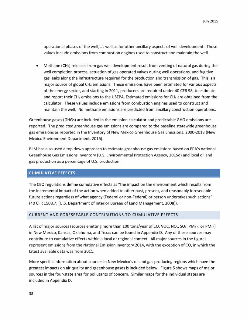
July 2015
38
operational phases of the well, as well as for other ancillary aspects of well development. These
values include emissions from combustion engines used to construct and maintain the well.
Methane (CH4) releases from gas well development result from venting of natural gas during the
well completion process, actuation of gas operated valves during well operations, and fugitive
gas leaks along the infrastructure required for the production and transmission of gas. This is a
major source of global CH4 emissions. These emissions have been estimated for various aspects
of the energy sector, and starting in 2011, producers are required under 40 CFR 98, to estimate
and report their CH4 emissions to the USEPA. Estimated emissions for CH4 are obtained from the
calculator. These values include emissions from combustion engines used to construct and
maintain the well. No methane emissions are predicted from ancillary construction operations.
Greenhouse gases (GHGs) are included in the emission calculator and predictable GHG emissions are
reported. The predicted greenhouse gas emissions are compared to the baseline statewide greenhouse
gas emissions as reported in the Inventory of New Mexico Greenhouse Gas Emissions: 2000-2013 (New
Mexico Environment Department, 2016).
BLM has also used a top down approach to estimate greenhouse gas emissions based on EPA’s national
Greenhouse Gas Emissions Inventory (U.S. Environmental Protection Agency, 2015d) and local oil and
gas production as a percentage of U.S. production.
CUMULATIVE EFFECTS
The CEQ regulations define cumulative effects as “the impact on the environment which results from
the incremental impact of the action when added to other past, present, and reasonably foreseeable
future actions regardless of what agency (Federal or non-Federal) or person undertakes such actions”
(40 CFR 1508.7; (U.S. Department of Interior Bureau of Land Management, 2008)).
CURRENT AND FORESEEABLE CONTRIBUTIONS TO CUMULATIVE EFFECTS
A list of major sources (sources emitting more than 100 tons/year of CO, VOC, NOx, SO2, PM2.5, or PM10)
in New Mexico, Kansas, Oklahoma, and Texas can be found in Appendix D. Any of these sources may
contribute to cumulative effects within a local or regional context. All major sources in the figures
represent emissions from the National Emission Inventory 2014, with the exception of CO, in which the
latest available data was from 2011.
More specific information about sources in New Mexico’s oil and gas producing regions which have the
greatest impacts on air quality and greenhouse gases is included below. Figure 5 shows maps of major
sources in the four-state area for pollutants of concern. Similar maps for the individual states are
included in Appendix D.

July 2015
39
Figure 5a. Major Emissions Sources (CO), New Mexico, Kansas, Oklahoma and Texas (U.S. Environmental
Protection Agency, 2016d)
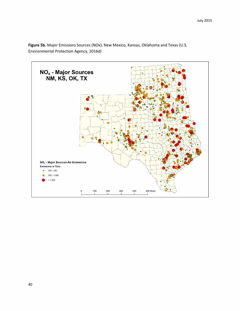
July 2015
40
Figure 5b. Major Emissions Sources (NOx), New Mexico, Kansas, Oklahoma and Texas (U.S.
Environmental Protection Agency, 2016d)

July 2015
41
Figure 5c. Major Emissions Sources (PM2.5), New Mexico, Kansas, Oklahoma and Texas (U.S.
Environmental Protection Agency, 2016d)
July 2015
42
Figure 5d. Major Emissions Sources (PM10), New Mexico, Kansas, Oklahoma and Texas (U.S.
Environmental Protection Agency, 2016d)
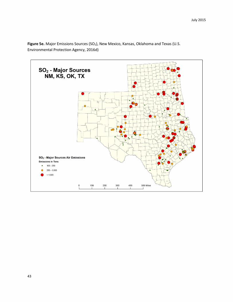
July 2015
43
Figure 5e. Major Emissions Sources (SO2), New Mexico, Kansas, Oklahoma and Texas (U.S.
Environmental Protection Agency, 2016d)

July 2015
44
Figure 5f. Major Emissions Sources (VOC), New Mexico, Kansas, Oklahoma and Texas (U.S.
Environmental Protection Agency, 2016d)
ELECTRICAL GENERATING UNITS
There are two coal-fired electrical generation units (EGUs) in the Four Corners area: the San Juan
Generating Station, located 15 miles west of Farmington, NM; and the Four Corners Power Plant,
located on Navajo Nation land in Fruitland, NM. These EGUs are the primary source of several criteria air
pollutants in the FFO area, including SO2 (85%), NOx (41%), and PM2.5 (3%) (U.S. Environmental
Protection Agency, 2016d). EGUs are responsible for 31% of New Mexico GHG emissions (New Mexico
Environment Department, 2016) and 31% of U.S. GHG emissions (U.S. Environmental Protection Agency,
2015d).
July 2015
45
In 2013, the New Mexico Environment Department, Public Service Company of New Mexico and EPA
agreed to meet the requirements of the federal regional haze rule through the shutdown of two units at
the San Juan Generating Station by the end of 2017. The agreement also requires the installation of
selective non-catalytic reduction technology on the remaining two units. This will result in significant
reductions from current emissions levels of many pollutants: a 67% reduction in SO2, 62% reduction in
NOx, 50% reduction in particulate matter, 44% reduction in CO, 51% reduction in VOC, 50% reduction in
CO2 and 50% reduction in mercury. The New Mexico Environmental Improvement Board approved a
revision to the State Implementation Plan containing the agreement requirements in the fall of 2013.
In December 2013, three coal-fired generators were shut down at the Four Corners Power Plant as part
of a plan to meet the requirements of the federal regional haze rule. The remaining two coal-fired
generators will have selective catalytic reduction technology installed by 2018. These changes satisfy
Best Available Retrofit Technology requirements from EPA. This will result in significant reductions from
current emissions levels of many pollutants: a 36% reduction in NOx, a 61% reduction in mercury, a 43%
reduction in particulate matter, a 30% reduction in CO2, and a 24% reduction in SO2.
In Texas, NOx emissions from EGUs in ozone nonattainment areas (Beaumont-Port Arthur, Dallas-Fort
Worth and Houston-Galveston-Brazoria) are required to limit NOx emissions from utility boilers,
auxiliary steam boilers, stationary gas turbines and duct burners under 30 TAC Chapter 117, Subchapter
C. The Texas proposed regional haze SIP did not require BART-eligible EGUs to install controls because
the state of Texas determined impact of each plant’s emissions did not significantly degrade visibility in
a Class I area, or facilities had already reduced emissions or shut down units. On December 16, 2014,
EPA proposed to partially disapprove the Texas regional haze SIP and also propose a Federal
Implementation Plan to require SO2 emissions reductions at fifteen Texas BART-eligible sources.
In Oklahoma, Tulsa Public Service Company of Oklahoma will retire one coal-fired unit at Oologah by
April 2016 and install a dry sorbent injection system on a second coal-fired unit at the same time. The
second unit will be shut down by December 31, 2026 to meet the requirements of the federal regional
haze rule. In 2016, SO2 emissions will be reduced by 78% and NO2 emissions will be reduced by 81%. In
2011, EPA disapproved the Oklahoma SIP revision plan for controls at Oklahoma Gas and Electric’s
Sooner and Muskogee Units and the AEP/PSO Northeastern Units 3 and 4. EPA determined that dry
scrubber control technology was needed at these units to meet federal haze rule requirements. The
disapproval has been challenged by the State of Oklahoma, upheld by the courts and has now been
appealed to the Supreme Court by the State of Oklahoma. Oklahoma submitted a SIP revision in 2013
that was approved by EPA in March 2014 that revises the BART determination for AEP/PSO Units 3 and
4. The revised determination included short-term compliance with emissions limits, shut down of one
of the units by April 16, 2016, and shut down of the other unit by December 31, 2026.
In Kansas, emissions at four coal-fired units were significantly reduced as a result of the federal regional
haze rule. At Kansas City Power and Electric’s La Cygne plant, SCR was installed on both units and

July 2015
46
scrubbers were installed. This resulted in 83% reduction in NOx emissions and 82% reduction in SO2
emissions. At Westar’s Jeffrey coal-fired units, low-NOx burner installation and switching to natural gas
combustion resulted in an 82% reduction in NOx emissions and a 34% reduction in SO2 emissions.
FOSSIL FUEL PRODUCTION
Fossil fuel production contributes to air pollutants and GHG emissions in the Farmington and Carlsbad
Field Office areas, especially San Juan, Northwestern Sandoval, Eddy, Lea, and Chaves counties as well as
in parts of Oklahoma, Kansas and Texas. This includes oil and gas production, natural gas compressor
stations and pipelines, gas plants, and petroleum refining. Coal mining is also occurring in the FFO and
Oklahoma Field Office (OFO) areas. Potash mining in the CFO area also contributes to air contaminant
and GHG emissions.
The BLM has jurisdiction over federal oil and gas exploration and production on Federal and Indian
mineral estate. Once produced oil or gas leaves the well location (via pipeline or tanker truck), the BLM
no longer has jurisdiction over these products.
There are currently approximately 16,289 oil and gas wells on federal mineral estate in the counties
within FFO (San Juan, Rio Arriba, Sandoval, and McKinley) that are categorized as active, new or
temporarily abandoned (Petroleum Recovery Research Center, 2015). If oil and gas wells with private
(fee), state-owned, or Indian mineral estate in these counties are included, there is a total of 23,364
active, producing, and inactive (shut in or temporarily abandoned) wells in the area. Table 6 shows 2012
oil and gas production on federal leases by state and as a percentage of U.S. production.
There are currently approximately 17,798 oil and gas wells on federal mineral estate in the counties
within CFO (Eddy, Lea and Chavez) that are categorized as active, new or temporarily abandoned
(Petroleum Recovery Research Center, 2015). If oil and gas wells with private (fee), state-owned, or
Indian mineral estate in these counties are included, there are approximately 40,488 active, producing,
and inactive (shut in or temporarily abandoned) wells in the area.
BLM’s Automated Fluid Minerals Support System (AFMSS) provides information about federal mineral
estate in Kansas, Oklahoma and Texas for fiscal year 2014 (U.S. Department of the Interior, 2015). There
were approximately 413 oil and gas wells on federal mineral estate and 78,131 total oil and gas wells in
Kansas (calendar year 2012) (Kansas Geological Survey, 2015); 469 oil and gas wells on federal mineral
estate and 180,000 total oil and gas wells in Oklahoma (calendar year 2011) (Oklahoma Corporation
Commission, 2011); there were 556 oil and gas wells on federal mineral estate and 319,604 total active
oil and gas wells in Texas (calendar year 2012) (Railroad Commission of Texas, 2015).

July 2015
47
Table 6: 2014 Oil and Gas Production (Petroleum Recovery Research Center, 2015), (U.S. Department of Interior Office of Natural Resources Revenue, 2015), (U.S. Energy Information Administration, 2015), (U.S. Energy Information Administration, 2015a)
*2014 data
Table 7 shows the estimated GHG emissions for oil and gas field production for the U.S., New Mexico,
Kansas, Oklahoma and Texas and for Federal leases in those states including New Mexico portions of the
San Juan and Permian Basins. Because oil and gas leaves the custody and jurisdiction of the BLM after
the production phase and before processing or refining, only emissions from the production phases are
considered here. It should also be remembered that following EPA protocols, these numbers do not
Location
Oil (bbl)
% U.S. Total
Gas (MMcf)
% U.S. Total
United States 3,161,866,000 100 27,271,326 100
New Mexico 121,206,000 3.83 1,267,646 4.65
Federal leases NM 64,889,645 2.05 770,572 2.83
San Juan Basin 4,494,909 0.14 524,408 1.92
Permian Basin 60,394,736 1.91 246,164 0.90
Kansas 49,521,000 1.57 292,467* 1.07
Federal leases KS 267,542 0.01 4,807 0.02
Oklahoma 128,026,000 4.05 2,310,114 8.47
Federal leases OK 253,262 0.01 12,267 0.04
Texas (onshore) 1,154,855,000 36.52 8,627,615 31.64
Federal leases TX 411,954 0.01 35,086 0.13
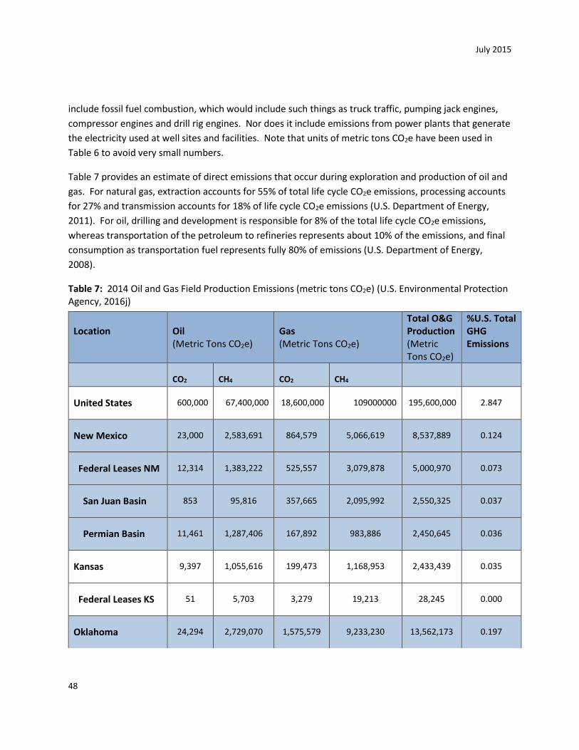
July 2015
48
include fossil fuel combustion, which would include such things as truck traffic, pumping jack engines,
compressor engines and drill rig engines. Nor does it include emissions from power plants that generate
the electricity used at well sites and facilities. Note that units of metric tons CO2e have been used in
Table 6 to avoid very small numbers.
Table 7 provides an estimate of direct emissions that occur during exploration and production of oil and
gas. For natural gas, extraction accounts for 55% of total life cycle CO2e emissions, processing accounts
for 27% and transmission accounts for 18% of life cycle CO2e emissions (U.S. Department of Energy,
2011). For oil, drilling and development is responsible for 8% of the total life cycle CO2e emissions,
whereas transportation of the petroleum to refineries represents about 10% of the emissions, and final
consumption as transportation fuel represents fully 80% of emissions (U.S. Department of Energy,
2008).
Table 7: 2014 Oil and Gas Field Production Emissions (metric tons CO2e) (U.S. Environmental Protection Agency, 2016j)
Location Oil
(Metric Tons CO2e) Gas (Metric Tons CO2e)
Total O&G Production (Metric Tons CO2e)
%U.S. Total GHG Emissions
CO2 CH4 CO2 CH4
United States 600,000 67,400,000 18,600,000 109000000 195,600,000 2.847
New Mexico 23,000 2,583,691 864,579 5,066,619 8,537,889 0.124
Federal Leases NM 12,314 1,383,222 525,557 3,079,878 5,000,970 0.073
San Juan Basin 853 95,816 357,665 2,095,992 2,550,325 0.037
Permian Basin 11,461 1,287,406 167,892 983,886 2,450,645 0.036
Kansas 9,397 1,055,616 199,473 1,168,953 2,433,439 0.035
Federal Leases KS 51 5,703 3,279 19,213 28,245 0.000
Oklahoma 24,294 2,729,070 1,575,579 9,233,230 13,562,173 0.197

July 2015
49
The New Mexico Greenhouse Gas Inventory and Reference Case Projection 1990-2020 (New Mexico
Environment Department, 2006) estimates that approximately 17.3 million metric tons of GHGs from
the natural gas industry and 2.3 million metric tons of GHGs from the oil industry were projected in 2010
as a result of oil and natural gas production, processing, transmission and distribution. As of June 9,
2015, there were 20,339 active oil wells and 26,387 active gas wells in New Mexico (Petroleum Recovery
Research Center, 2015).
Compressor engines link the natural gas pipeline infrastructure that transports natural gas from its
source to points of consumption. Table 8 shows the greenhouse gas emissions from compressor
stations and gas plants for each state from the 2013 Greenhouse Gas Facility Level Information on
Greenhouse Gases Tool (FLIGHT). Some gas plants and compressor stations’ emissions may not be
reported to FLIGHT because emissions from the plant or station do not exceed EPA’s GHG reporting
threshold.
Table 8: 2014 Greenhouse gas emissions from gas plants and compressor stations (U.S. Environmental
Protection Agency, 2016h)
State Number of
reporting
compressor
stations
Total GHG
emissions
from
reporting
compressor
stations
(MMT CO2e)
%U.S.
Total
reported
Compressor
Station
GHG
Emissions
Number of
reporting
gas plants
Total GHG
emissions
from
reporting
gas plants
(MMT
CO2e)
%U.S.
Total
reported
Gas Plant
GHG
Emissions
New Mexico 6 0.33 1.5 26 5.3 8.83
Texas 49 2.3 10.4 207 21.0 35.0
Oklahoma 15 0.50 2.27 49 2.8 4.67
Federal Leases OK 48 5,399 8,367 49,030 62,843 0.001
Texas 219,147 24,617,497 5,884,336 34,483,473 65,204,453 0.949
Federal Leases TX 78 8,781 23,930 140,234 173,024 0.003

July 2015
50
Kansas 24 1.1 5.0 5 0.60 1.0
Emissions from processing, transmission and storage and distribution in the U.S. totaled 98 million
metric tons of CO2e in 2013, which was about 3% of total U.S. GHG emissions reported to EPA in 2013
(U.S. Environmental Protection Agency, 2016h).
In 2015, EPA Natural Gas Star partner companies operate 51% of the active federal wells in the New
Mexico portion of the San Juan Basin and 13% of the active federal wells in the New Mexico portion of
the Permian Basin. In Kansas, Natural Gas Star partner companies operate 5% of the active federal
wells; in Oklahoma, Natural Gas Star partner companies operate 11% of the active federal wells and in
Texas, Natural Gas Star partner companies operate 33% of the active federal wells (Petroleum Recovery
Research Center, 2015) (U.S. Department of Interior Bureau of Land Management, 2014). EPA has
found Natural Gas Star partners’ actions to result in measurable decreases in GHG emissions since the
program’s implementation.
Crude oil produced throughout the BLM-NM area is transported by pipeline and/or tanker truck to
refineries where the oil is processed into various types of fuel. Table 9 shows the greenhouse gas
emissions from refineries in each BLM-NM state.
Table 9: 2014 Greenhouse gas emissions from refineries (U.S. Environmental Protection Agency, 2016h)
State Number of Reporting
Refineries
Total GHG emissions
from reporting
compressor stations
(MMT CO2e)
%U.S. Total reported
Refinery GHG
Emissions
New Mexico 3 0.95 0.54
Texas 29 55 31.4
Oklahoma 5 4.7 2.7
Kansas 3 2.8 1.6
July 2015
51
There are two refineries in the CFO area, one in Artesia and one in Lovington. There is one refinery near
Gallup, NM operating in the FFO area. In Kansas, there are three refineries, Oklahoma has five refineries
and Texas has twenty-eight refineries. Transportation and processing of crude oil and petroleum
products result in emissions of various hazardous air pollutants, criteria pollutants, and GHGs. In 2013,
greenhouse gas emissions from refineries accounted for 177 million metric tons CO2e emitted (U.S.
Environmental Protection Agency, 2016h), which is 5.6% of the total GHG emissions reported to EPA.
Potash mining is another major industry in the CFO area. There are two mining companies operating 4
potash processing plants in the CFO area. Potash production produces emissions of various hazardous
air pollutants and criteria pollutants. In 2013, potash mines in southeastern New Mexico emitted
97,726 metric tons of CO2e cumulatively. This is 0.001% of total greenhouse gas emissions (U.S.
Environmental Protection Agency, 2016h).
Coal mining is another major industry in San Juan County. BHP Billiton operates two coal mines in
northwestern New Mexico that provide coal to the San Juan Generating Station and the Four Corners
Power Plant. Coal production produces emissions of various hazardous air pollutants, criteria pollutants,
and CH4. In 2013, coal mining in the U.S. contributed 63.2 million metric tons CO2e, which is 10.8% of
total U.S. CH4 emissions, and 1.1% of total U.S. GHG emissions (U.S. Environmental Protection Agency,
2016j).
TRANSPORTATION
Another primary source of emissions that impact air quality is vehicular travel. The number of vehicles,
miles traveled, types of vehicles in use, and the condition of road surfacing, all factor into the emissions
from vehicular travel. On and off-road vehicles produce exhaust which contains NOx, VOCs, CO, PM and
HAPs.
In 2013, fossil fuel combustion associated with transportation contributed 1,801.7 million metric tons
CO2e to total U.S. GHG emissions, which accounted for 27% of U.S. GHG emissions that year (U.S.
Environmental Protection Agency, 2016j). Over 90% of the fuel used for transportation is petroleum
based. Although it is expected that vehicle fuel efficiency and increased use of public transportation will
reduce vehicle emissions, these reductions may eventually be offset by an increased number of vehicles
in use due to population growth in the region.
CLIMATE CHANGE AND GHG EMISSIONS
Secretarial Order 3289, issued on September 14, 2009, established a Department-wide approach for
applying scientific tools to increase understanding of climate change and to coordinate an effective
response to its impacts on tribes, and on the land, water, ocean, fish and wildlife, and cultural heritage
resources the Department manages. The Secretarial Order states that one must “consider and analyze
July 2015
52
potential climate change impacts when undertaking long-range planning exercises, setting priorities for
scientific research and investigations, and/or when making major decisions affecting DOI resources.”
BLM does recognize the importance of climate change and the potential effects it could have on natural
and socioeconomic environments. Since the assessment of GHG emissions and climate change is in its
formative phase it is currently not feasible to predict the exact impacts the Proposed Action would have
on climate and projected
For the purpose of NEPA analysis, EPA emission factors can be used to include a qualitative and
quantitative analysis of possible greenhouse gas emissions that could occur as a result of reasonably
foreseeable coal, oil, gas or other development connected to federal land and resource management
use. Estimates are made based on readily available data and reasonable assumptions about potential
future development. More detailed emissions would be available and calculated at a site specific level of
analysis such as those that occur at an APD stage.
Existing conditions of air resources in any given location are the result of numerous complex factors,
both natural and human caused. Natural factors contributing to the current condition of air resources
include existing climate resulting from long-term atmospheric weather patterns, soil types, and
vegetation types. Anthropogenic factors contributing to the current condition of air resources include
long-term human habitation, growing human populations, transportation methods and patterns,
recreational activities, economic patterns, the presence of power plants and other industrial sources.
The presence of natural resource (i.e. oil and natural gas) extraction and processing on some BLM lands
also impact air quality and greenhouse gas emissions.
The primary sources of greenhouse gas emissions could include the following:
● Fossil fuel combustion for construction and operation of oil and gas facilities – vehicles driving to
and from production sites, engines that drive drill rigs, etc. These produce CO2 in quantities that
vary depending on the age, types, and conditions of the equipment as well as the targeted
formation, locations of wells with respect to processing facilities and pipelines, and other site-
specific factors.
● Fugitive CH4 – CH4 that escapes from wells (both gas and oil), oil storage, and various types of
processing equipment. This is a major source of global CH4 emissions. These emissions have
been estimated for various aspects of the energy sector, and starting in 2011, producers are
required under 40 C.F.R. §98, to estimate and report their CH4 emissions to the EPA.
● Combustion of produced oil and gas – it is expected that operations will produce marketable
quantities of oil and/or gas. Combustion of the oil and/or gas would release CO2 into the
atmosphere. Fossil fuel combustion is the largest source of global CO2.
Direct GHG Emissions
July 2015
53
Direct greenhouse gas emissions from speculative future oil and gas well production and associated
activities of the proposed action are summarized in the respective NEPA document. Total Greenhouse
Gas Warming Potential (GWP), which includes direct emissions of carbon dioxide, methane, and nitrous
oxide from an oil or gas producing well is calculated.
Indirect GHG Emissions
Indirect GHG emissions are estimated based on speculative annual oil, gas, and/or natural gas liquids
from the proposed action. Indirect GHG emissions are calculated only for carbon dioxide based on
combustion of the product. Emission factors are applied to the per-barrel or per-cubic foot unit of the
reasonably foreseeable development estimates. Emission factors used in BLM GHG Indirect Greenhouse
Gas Emissions are included below.
Oil indirect emission factor: 0.43 MT CO2 per Barrel (EIA, 2006),
Gas indirect emission factor: 0.054717 MT of CO2 per Mcf (U.S. Environmental Protection Agency,
2016k)
Natural Gas Liquids indirect emission factor 13.7 pounds of CO2 per gallon of Prop/Buta mix (EIA, 2006)
End Uses
Estimating direct and indirect GHG emissions attempt to provide a complete GHG lifecycle of a well from
site inspection to possible emissions through combustion. A rough estimate was possible using publicly
available information and using estimates from future production for reasonably foreseeable
development. With respect to the rough estimates of indirect CO2 emissions, it should be noted that it is
a difficult to discern with certainty what end uses for the fuels extracted from a particular leasehold
might be reasonably foreseeable. For instance, some end uses of fossil fuels extracted from Federal
leases include: combustion of transportation fuels, fuel oils for heating and electricity generation, as
well as production of asphalt and road oil, and the feedstocks used to make chemicals, plastics, and
synthetic materials. At this time, there is some uncertainty with regard to the actual development that
may occur.
It is important to note that the BLM does not exercise control over the specific end use of the oil and gas
produced from any individual federal lease. The BLM has no authority to direct or regulate the end use
of the produced oil and/or gas. As a result, the BLM can only provide an estimate of potential GHG
emissions using national approximations of where or how the end use may occur because coal, oil,
condensate, and natural gas could be used for combustion of transportation fuels, fuel oils for heating
and electricity generation, as well as production of asphalt and road oil, and the feedstocks used to
make chemicals, plastics, and synthetic materials.

July 2015
54
Global, National And State GHG Emissions
It is useful to compare the relative and absolute contributions to climate change of different GHG
emissions, as well as emissions from different regions/countries or sources/sectors. There are several
different metrics that can be used for this comparison. The most common is Global Warming Potential
(GWP), a relative measure that compares the heat absorbing ability of a certain mass of a gas relative to
the same mass of carbon dioxide (CO2). A second metric that is gaining prominence is Global
Temperature change Potential (GTP). GTP is based on the change in global mean surface temperature at
a chosen point in time, relative to that caused by CO2. A number of other metrics may also be used, but
no single metric accurately compares all consequences and the choice of metric is a value judgment
(Intergovernmental Panel on Climate Change (IPCC), 2013).
Global Warming Potential (GWP) is dependent both upon the heat-absorbing ability of a particular gas
and its atmospheric lifetime. A gas that is quickly removed from the atmosphere may have a high GWP
over a short period of time, but a lower impact over a longer time period. For example, methane gas
(CH4) has a GWP of 56 over a 20-year time horizon and a GWP of 21 over a 100-year time horizon
(Intergovernmental Panel on Climate Change (IPCC), 1996). This means that CH4 is 56- and 21-times
more potent than CO2 over these time periods. The most potent GHG ever evaluated is sulfur
hexafluoride (SF6). Although trace gases such as SF6 are present in low concentrations, they have high
GWPs because they are both very effective at trapping heat and have very long atmospheric lifetimes.
In accordance with international GHG reporting standards under the United Nations Framework
Convention on Climate Change (UNFCCC) and in order to maintain consistent comparisons over the
years, official GHG emission estimates for the United States are reported based on the GWP values given
in the IPCC Second Assessment Report (SAR) (Intergovernmental Panel on Climate Change (IPCC), 1996).
These values have been revised in the IPCC Third (Intergovernmental Panel on Climate Change (IPCC),
2001), Fourth (Intergovernmental Panel on Climate Change (IPCC), 2007), and Fifth (Intergovernmental
Panel on Climate Change (IPCC), 2013) Assessment Reports as our level of scientific understanding
increases. The atmospheric lifetimes and GWPs for the major GHGs over a 100-year time horizon from
the Second Assessment Report (SAR) are listed below in Table 10.
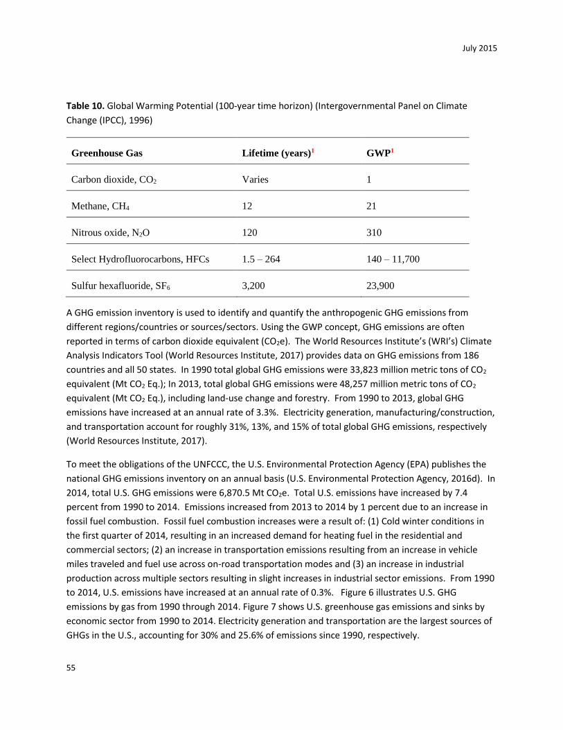
July 2015
55
Table 10. Global Warming Potential (100-year time horizon) (Intergovernmental Panel on Climate
Change (IPCC), 1996)
Greenhouse Gas Lifetime (years)1 GWP1
Carbon dioxide, CO2 Varies 1
Methane, CH4 12 21
Nitrous oxide, N2O 120 310
Select Hydrofluorocarbons, HFCs 1.5 – 264 140 – 11,700
Sulfur hexafluoride, SF6 3,200 23,900
A GHG emission inventory is used to identify and quantify the anthropogenic GHG emissions from
different regions/countries or sources/sectors. Using the GWP concept, GHG emissions are often
reported in terms of carbon dioxide equivalent (CO2e). The World Resources Institute’s (WRI’s) Climate
Analysis Indicators Tool (World Resources Institute, 2017) provides data on GHG emissions from 186
countries and all 50 states. In 1990 total global GHG emissions were 33,823 million metric tons of CO2
equivalent (Mt CO2 Eq.); In 2013, total global GHG emissions were 48,257 million metric tons of CO2
equivalent (Mt CO2 Eq.), including land-use change and forestry. From 1990 to 2013, global GHG
emissions have increased at an annual rate of 3.3%. Electricity generation, manufacturing/construction,
and transportation account for roughly 31%, 13%, and 15% of total global GHG emissions, respectively
(World Resources Institute, 2017).
To meet the obligations of the UNFCCC, the U.S. Environmental Protection Agency (EPA) publishes the
national GHG emissions inventory on an annual basis (U.S. Environmental Protection Agency, 2016d). In
2014, total U.S. GHG emissions were 6,870.5 Mt CO2e. Total U.S. emissions have increased by 7.4
percent from 1990 to 2014. Emissions increased from 2013 to 2014 by 1 percent due to an increase in
fossil fuel combustion. Fossil fuel combustion increases were a result of: (1) Cold winter conditions in
the first quarter of 2014, resulting in an increased demand for heating fuel in the residential and
commercial sectors; (2) an increase in transportation emissions resulting from an increase in vehicle
miles traveled and fuel use across on-road transportation modes and (3) an increase in industrial
production across multiple sectors resulting in slight increases in industrial sector emissions. From 1990
to 2014, U.S. emissions have increased at an annual rate of 0.3%. Figure 6 illustrates U.S. GHG
emissions by gas from 1990 through 2014. Figure 7 shows U.S. greenhouse gas emissions and sinks by
economic sector from 1990 to 2014. Electricity generation and transportation are the largest sources of
GHGs in the U.S., accounting for 30% and 25.6% of emissions since 1990, respectively.
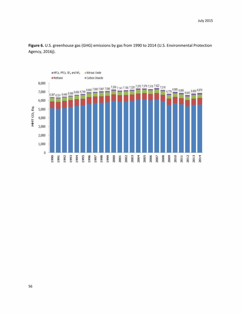
July 2015
56
Figure 6. U.S. greenhouse gas (GHG) emissions by gas from 1990 to 2014 (U.S. Environmental Protection
Agency, 2016j).

July 2015
57
Figure 7. U.S. greenhouse gas (GHG) emissions and sinks by economic sector from 1990 to 2014 (U.S.
Environmental Protection Agency, 2016j).
Globally, emissions of CO2 from flaring of unused gas during oil production decreased by about a quarter
between 2003 and 2011; however, flaring emissions for the U.S. are on the rise and increased by 50% in
2011 because of the significant increase in fracking for shale oil production and the flaring of co-
produced natural gas (Olivier, 2012).
The Inventory of New Mexico Greenhouse Gas Emissions: 2000-2013 (New Mexico Environment
Department, 2016) lists total statewide gross GHG emissions in 2013 as 80.9 Mt CO2 Eq. For 2013, New
Mexico’s Environment Department reported that the primary contributors to the state’s GHG emissions
were electricity generation (35%), the fossil fuel industry (26%), and transportation (17%) (New Mexico
Environment Department, 2016). In 2012, WRI’s CAIT reports that New Mexico’s GHG emissions were
75.5 Mt CO2 Eq. (World Resources Institute, 2017). Electricity generation, transportation, and fugitive
sources account for around 29%, 14%, and 11% of New Mexico’s GHG emissions in 2012 (World

July 2015
58
Resources Institute, 2017). According to the New Mexico Greenhouse Gas Inventory and Reference Case
Projections, 1990-2020, GHG emissions were expected to continue increasing (New Mexico Environment
Department, 2006). From 1990 to 2012, New Mexico’s GHG emissions have decreased at an annual
rate of 0.45% (New Mexico Environment Department, 2016).
With respect to GHGs emitted by oil and gas development, carbon dioxide (CO2) is produced during the
burning of fossil fuels to run internal combustion engines which may be used in drilling, transportation,
pumping and compression. Carbon dioxide may be a significant component of natural gas, especially
coalbed methane, and is vented during field operations or processing. Carbon dioxide is also used in
enhanced oil production processes and may be released or escape to the atmosphere during those
processes. Methane (CH4) is the primary component of natural gas and is released to the atmosphere
during both oil and gas production either intentionally during production when it cannot be captured, or
accidentally through leaks and fugitive emissions.
The EPA’s national GHG emissions inventory describes “Natural Gas Systems” and “Petroleum Systems”
as two of the major sources of U.S. GHG emissions. The inventory identifies the contributions of natural
gas and petroleum systems to total carbon dioxide (CO2) and methane (CH4) emissions (natural gas and
petroleum systems do not produce noteworthy amounts of any other GHGs). Within the larger category
of “Natural Gas Systems”, the EPA identifies emissions occurring during distinct stages of operation,
including field production, processing, transmission and storage, and distribution.
Table 11. U.S. Inventory of Greenhouse Gas Emissions for oil and gas subsectors 2014 (U.S.
Environmental Protection Agency, 2016j)
Sector Subsector
2014 GHG Emissions (MMTCO2e) % of U.S.
Total
GHGs
CO2 CH4 N20
Total
GHGs
Natural Gas
Systems
Total 42.4
176.1
*
218.2
3.18%
Field production 18.6 109.0 * 127.6 1.86%
Processing 23.7 24.0 * 47.7 0.69%
Transmission and storage * 32.1 * 32.1 0.47%
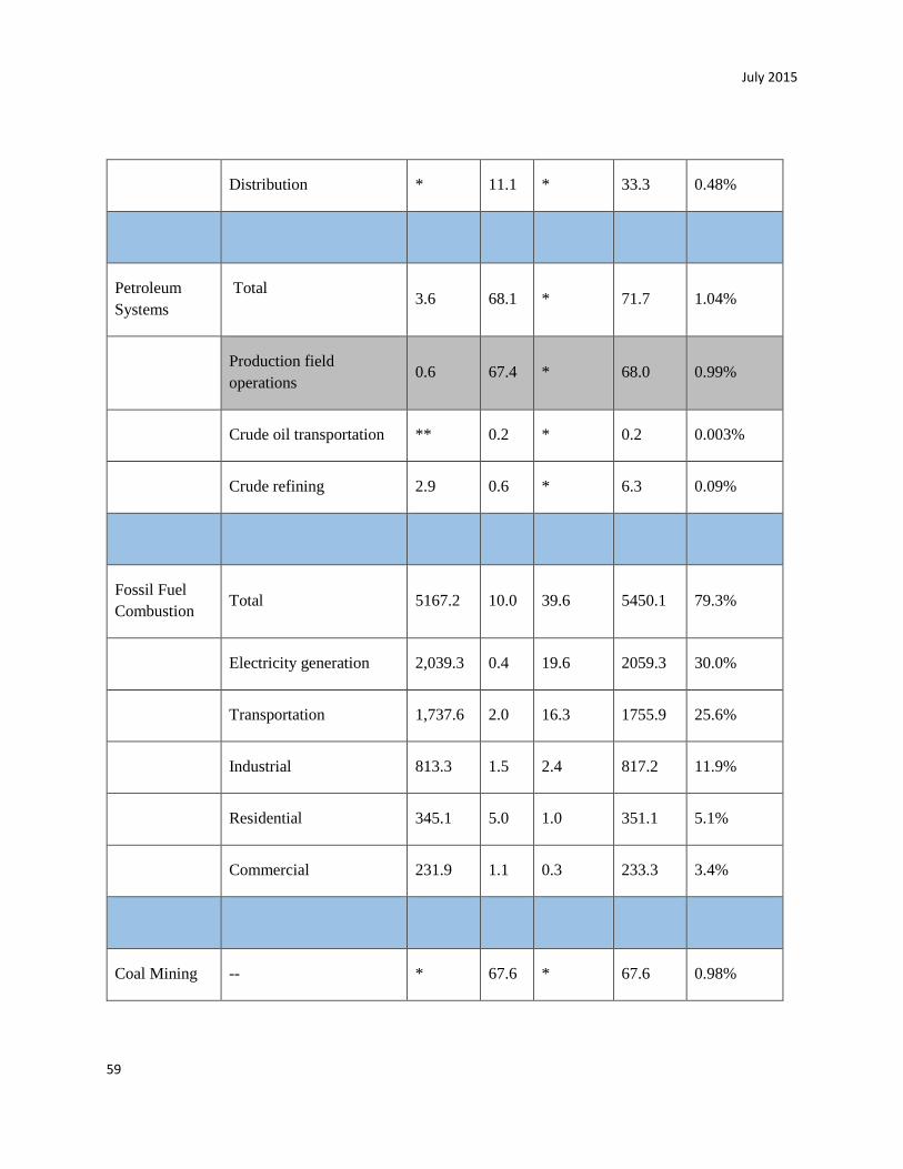
July 2015
59
Distribution * 11.1 * 33.3 0.48%
Petroleum
Systems
Total 3.6 68.1 * 71.7 1.04%
Production field
operations 0.6 67.4 * 68.0 0.99%
Crude oil transportation ** 0.2 * 0.2 0.003%
Crude refining 2.9 0.6 * 6.3 0.09%
Fossil Fuel
Combustion Total 5167.2 10.0 39.6 5450.1 79.3%
Electricity generation 2,039.3 0.4 19.6 2059.3 30.0%
Transportation 1,737.6 2.0 16.3 1755.9 25.6%
Industrial 813.3 1.5 2.4 817.2 11.9%
Residential 345.1 5.0 1.0 351.1 5.1%
Commercial 231.9 1.1 0.3 233.3 3.4%
Coal Mining -- * 67.6 * 67.6 0.98%
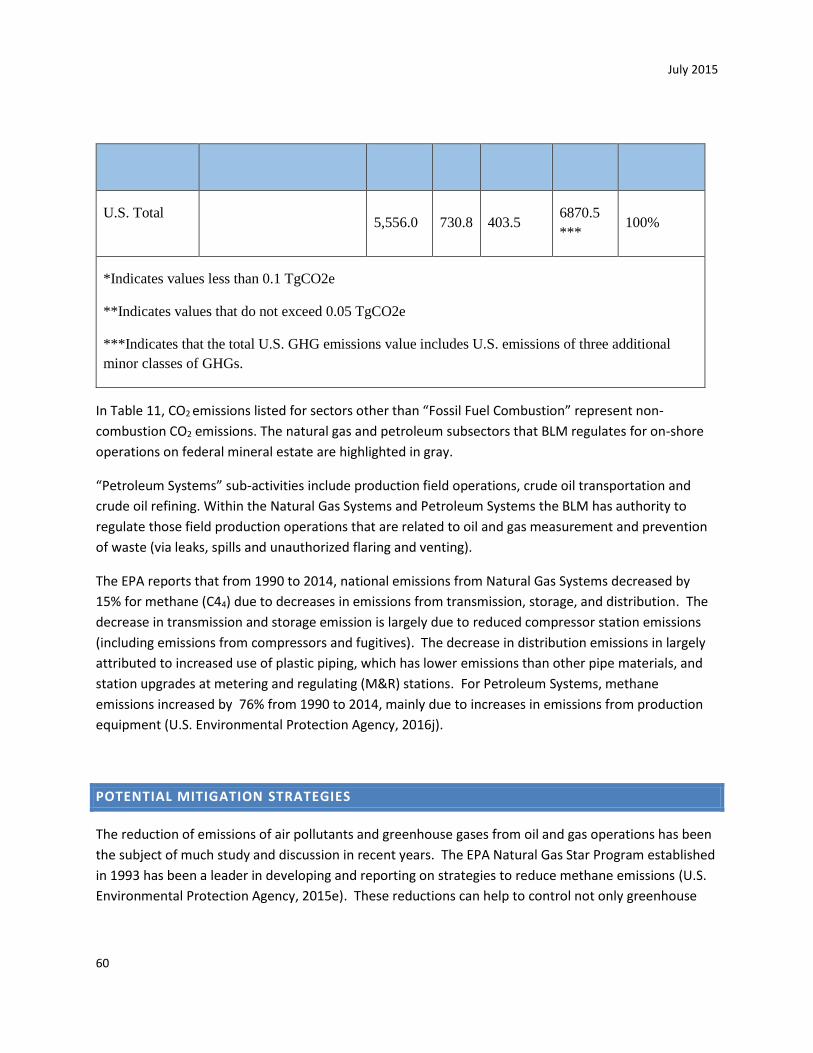
July 2015
60
U.S. Total 5,556.0 730.8 403.5
6870.5
*** 100%
*Indicates values less than 0.1 TgCO2e
**Indicates values that do not exceed 0.05 TgCO2e
***Indicates that the total U.S. GHG emissions value includes U.S. emissions of three additional
minor classes of GHGs.
In Table 11, CO2 emissions listed for sectors other than “Fossil Fuel Combustion” represent non-
combustion CO2 emissions. The natural gas and petroleum subsectors that BLM regulates for on-shore
operations on federal mineral estate are highlighted in gray.
“Petroleum Systems” sub-activities include production field operations, crude oil transportation and
crude oil refining. Within the Natural Gas Systems and Petroleum Systems the BLM has authority to
regulate those field production operations that are related to oil and gas measurement and prevention
of waste (via leaks, spills and unauthorized flaring and venting).
The EPA reports that from 1990 to 2014, national emissions from Natural Gas Systems decreased by
15% for methane (C44) due to decreases in emissions from transmission, storage, and distribution. The
decrease in transmission and storage emission is largely due to reduced compressor station emissions
(including emissions from compressors and fugitives). The decrease in distribution emissions in largely
attributed to increased use of plastic piping, which has lower emissions than other pipe materials, and
station upgrades at metering and regulating (M&R) stations. For Petroleum Systems, methane
emissions increased by 76% from 1990 to 2014, mainly due to increases in emissions from production
equipment (U.S. Environmental Protection Agency, 2016j).
POTENTIAL MITIGATION STRATEGIES
The reduction of emissions of air pollutants and greenhouse gases from oil and gas operations has been
the subject of much study and discussion in recent years. The EPA Natural Gas Star Program established
in 1993 has been a leader in developing and reporting on strategies to reduce methane emissions (U.S.
Environmental Protection Agency, 2015e). These reductions can help to control not only greenhouse
July 2015
61
gases but also VOCs, which contribute to ozone formation. Numerous opportunities for emissions
reduction, including costs to implement, are documented on EPA’s the Natural Gas Star website.
A report by the Government Accountability Office (GAO) noted that opportunities exist for capturing
fugitive emissions from venting and flaring of natural gas on wells under federal jurisdiction (U.S.
Government Accountability Office, 2010). A report prepared for BLM in Montana includes an entire
chapter on reduction of emissions of greenhouse gases (URS Corporation, 2010a). Another report
recently issued by the U.S. Forest Service summarizes and builds on work originally done by BLM to
identify Best Management Practices for protection of air quality during oil and gas development and
production (U.S. Forest Service, 2011).
While it is beyond the scope of this report to detail the wide range of mitigation strategies available it
must be understood that for the most part these strategies must be applied on a case by case basis at
the project level. Some broader range strategies applied within the BLM New Mexico State Office
jurisdiction are discussed below.
FOUR CORNERS AIR QUALITY TASK FORCE
In 2002, the State of New Mexico Environment Department and local governments convened to sign an
Early Action Compact (EAC) for ozone under a US EPA program that required commitment for state and
local action to resolving ozone issues prior to a nonattainment designation. In 2005, the states of
Colorado and New Mexico convened a group of stakeholders, then known as the Four Corners Air
Quality Task Force (Task Force), to address air quality issues in the Four Corners region in light of
continued energy development and growth in the region and consider options for mitigating air
pollution. A report detailing a wide range of mitigation options was published in November 2007 (Four
Corners Air Quality Task Force, 2007).
In 2008, its task complete, the group became known as the Four Corners Air Quality Group (FCAQG) and
continued on as a forum for discussion of existing air quality issues and potential solutions. The FCAQG
is currently comprised of more than 100 members and 150 interested parties representing a wide range
of perspectives on air quality in the Four Corners region. Members include private citizens,
representatives from public interest groups, universities, industry, state, tribal and local governments,
and federal agencies. The BLM has been an active participant from the beginning and maintains a
representative on the steering committee.
IR CAMERAS
The BLM has two Infrared Cameras which are being used to detect leaks and fugitive emissions. BLM
inspectors carry these cameras into the field and have been able to alert operators of equipment

July 2015
62
requiring repair or maintenance. At this time the cameras are being used in an advisory rather than a
regulatory role.
FOUR CORNERS METHANE HOTSPOT
Very recently, pioneering research using space-borne (satellite and aircraft) determination of methane
concentrations has indicated anomalously large methane concentrations may occur in the Four Corners
region (Kort, et al., 2014). A subsequent study (Schneising, et al., 2014) indicated larger anomalies over
other oil and gas basins in the U.S. Methane is 34 times more potent at trapping greenhouse gas
emissions than CO2 when considering a time horizon of 100 years (Intergovernmental Panel on Climate
Change, 2013). While space-borne studies can determine the pollutant concentration in a column of air,
these studies cannot pinpoint the specific sources of air pollution. Further study is required to
determine the sources responsible for methane concentrations in the Four Corners region; however, it is
known that a significant amount of methane is emitted during oil and gas well completion (Howarth,
Santoro, & A.Ingraffea, 2011). Methane is also emitted from process equipment, such as pneumatic
controllers and liquid unloadings, at oil and gas production sites. Ground-based, direct source
monitoring of pneumatic controllers conducted by the Center for Energy and Environmental Resources
(Allen, et al., 2014) show that methane emissions from controllers exhibit a wide range of emissions and
a small subset of pneumatic controllers emitted more methane than most. Emissions measured in the
study varied significantly by region of the U.S., the application of the controller and whether the
controller was continuous or intermittently venting. The Center for Energy and Environmental
Resources had similar findings of variability of methane emissions from liquid unloading (Allen, et al.,
2014a). In October 2012, USEPA promulgated air quality regulations controlling VOC emissions at
hydraulically fractured gas wells. These rules require air pollution mitigation measures that reduce the
emissions of volatile organic compounds. These same mitigation measures have a co-benefit of
reducing methane emissions. In April 2015, several researchers conducted further ground-based and
space-borne studies utilizing emerging pollutant measurement technology. The results of these studies
may help to pinpoint significant, specific sources of methane emissions in the region.
KANSAS, OKLAHOMA AND TEXAS
The BLM has jurisdiction over mineral rights on federal lands managed by other agencies and on split
estate lands in Kansas, Texas and Oklahoma. A review of Table 6 above will show that oil and gas
production on federal leases is fairly small compared to production on other lands in these states. The
purpose of this chapter is to address air quality concerns and regulations that are unique to these states
and not already covered above.
July 2015
63
KANSAS
The regulatory authority for air quality in Kansas is the Kansas Department of Health and Environment,
Bureau of Air (http://www.kdheks.gov/bar/). The state does not have any ambient air quality standards
that differ from the NAAQS (Table 1). There are currently no non-attainment areas for any criteria
pollutant in the state of Kansas.
OKLAHOMA
The regulatory authority for air quality in Oklahoma is the Oklahoma Department of Environmental
Quality, Air Quality Division (http://www.deq.state.ok.us/AQDnew/ ). Oklahoma’s ambient air quality
standards are identical with the NAAQS (Table 1). There are currently no nonattainment areas in the
state of Oklahoma.
TEXAS
The regulatory authority for air quality in Texas is the Texas Commission on Environmental Quality
(TCEQ), Air Division. The state does not have any ambient air quality standards that differ from the
NAAQS (Table 1).
Non-Attainment Areas And Conformity Analysis
There are currently four non-attainment areas in Texas, one for PM10 (El Paso), two for ozone (Houston
area, Dallas-Fort Worth area) and a portion of Collin County is non-attainment for lead, according to the
TCEQ website (http://www.tceq.texas.gov). EPA’s conformity rule requires that all federal actions in a
non-attainment area must demonstrate conformity with the State Implementation Plan (SIP) for the
pollutant in question. If the agency can demonstrate that emissions for the action will fall below certain
established levels, known as de minimus, then no further analysis is necessary. In order to establish de
minimus an emissions inventory for the project is required. In the case of ozone, the emissions
inventory would include NOx and VOCs. If emissions are projected to be above de minimus levels
further analysis should be coordinated with the EPA and Texas CEQ.
The Houston-Galveston-Brazoria area was designated as severe nonattainment for 8 hour ozone based
on the 1997 standard in October 2008 and includes the following counties: Brazoria, Chambers, Fort
Bend, Galveston, Harris, Liberty, Montgomery, and Waller. De minimus values for both NOx and VOC in
this area are 25 tons/year.
The Dallas-Fort Worth ozone nonattainment area was designated in June 2004, is classified as moderate
and includes the following counties: Collin, Dallas, Denton, Tarrant, Ellis, Johnson, Kaufman, Parker, and
Rockwall. De minimus values in this area are 100 tons/yr for NOx and 50 tons/yr for VOC.

July 2015
64
AIR QUALITY MODELING FOR TEXAS
Numerous reports on air quality modeling projects done by and for the TCEQ, including modeling done
for the Dallas and Houston non-attainment areas can be accessed on the Air Division website
(http://www.tceq.texas.gov/airquality/airmod/am). The TCEQ has convened advisory groups in
southeastern Texas and Dallas-Fort Worth to assist the agency in addressing photochemical modeling
issues.
REFERENCES
Allen, D., Pacsi, A., Sullivan, D., Araiza, D. Z., Harrison, M., Keen, K., . . . Seinfeld, J. (2014). Methane Emissions from
Process Equipment at Natural Gas Production Sites in the United States: Pneumatic Controllers.
Environmental Science and Technology, es5040156.
Allen, D., Sullivan, D., Araiza, D. Z., A.Pacsi, Harrison, M., Keen, K., . . . Seinfeld, J. (2014a). Methane Emissions from
Process Equipment at Natural Gas Production Sites in the United States: Liquid Unloadings. Environmental
Science and Technology, es504015.
AMEC Environment and Infrastructure, Inc. (2014). Clean Air Status and Trends Network: 2012 Annual Report.
Research Triangle Park: USEPA.
Applied Enviro Solutions. (2011). Southeast New Mexico Inventory of Air Pollutant Emissions and Cumulative Air
Impact Analysis 2007. Carlsbad: BLM Carlsbad Field Office.
Bureau of Reclamation, Sandia National Laboratories, U.S. Army Corps of Engineers. (2013). West-Wide Climate
Risk Assessment: Upper Rio Grande Impact Assessment. Albuquerque: Bureau of Reclamation.
Cayan, D. (2013). The Southwest Cimate of the Future-Projections of Mean Climate. Washington, D.C.: National
Climate Assessment.
Colorado State University. (2014). VIEWS 2.0. Retrieved January 3, 2014, from Visibility Information Exchange
Website: http://views.cira.colostate.edu/web/Trends/
Council on Environmental Quality (CEQ). (2016). Final Guidance on Consideration of Greenhouse Gas Emissions and
the Effects of Climate Change in National Environmental Policy Act Reviews. Washington, D.C.: Council on
Environmental Quality.
EIA. (2006). Carbon Dioxide Coefficients. Retrieved from Energy Information Agency (EIA) Volume 2, Energy:
http://www.eia.gov/tools/faqs/faq.cfm?id=7&t=7
Environ. (2009). Air Quality Modeling Study for the Four Corners Region. Santa Fe: New Mexico Environment
Department Air Quality Bureau.

July 2015
65
ENVIRON International Corporation, Alpine Geophysics, LLC and University of North Carolina. (2013). Western
Regional Air Partnership (WRAP) West-wide Jump-start Air Quality Modeling Study (WestJumpAQMS). Fort
Collins: Western Regional Air Partnership.
Four Corners Air Quality Task Force. (2007). Report of Mitigation Options. Santa Fe: New Mexico Environment
Department.
Howarth, R., Santoro, R., & A.Ingraffea. (2011). Methane and the greenhouse-gas footprint of natural gas from
shale formations. Climate Change, 679-690.
Intergovernmental Panel on Climate Change (IPCC). (1996). Climate Change 1995: The Science of Climate Change,
Contribution of Working Group I to the Second Assessment Report of the Intergovernmental Panel on
Climate Change. Cambridge and New York: Cambridge University Press.
Intergovernmental Panel on Climate Change (IPCC). (2001). Climate Change 2001: The Scientific Basis, Contribution
of Working Group I to the Third Assessment Report of the Intergovernmental Panel on Climate Change.
Cambridge and New York: Cambridge University Press.
Intergovernmental Panel on Climate Change (IPCC). (2007). Climate Change 2007: The Physical Basis. Cambridge
and New York: Cambridge University Press.
Intergovernmental Panel on Climate Change (IPCC). (2013). Climate Change 2013: The Physical Science Basis,
Contribution of Working Group I to the Fifth Assessment Report of the Intergovernmental Panel on Climate
Change. Cambridge and New York: Cambridge University Press.
Intergovernmental Panel on Climate Change. (2013). Climate Change 2013: The Physical Science Basis. Cambridge:
Cambridge University Press.
Joint Science Academies. (2005). Joint Science Academies' Statement: Global Response to Climate Change. National
Academy of Sciences.
Kansas Geological Survey. (2015, April 21). State Production and Historical Info. Retrieved May 7, 2015, from KU
Kansas Geological Survey: http://www.kgs.ku.edu/PRS/petro/state.html
Karl, T. L. (2009). Global Climate Change Impacts in the United States. Cambridge: Cambridge University Press.
Kleinfelder West, Inc. (2013). Air Emissions Inventory Estimates for a Representative Oil and Gas Well in the
Western United States. Littleton: Kleinfelder.
Kort, E., Frankenberg, C., Costigan, K., Lindenmaier, R., Dubey, M., & Wunch, D. (2014). Four corners: The largest
US methane anomaly viewed from space. Geophysical Research Letters, 6898-6903.
Lusk, J. E. (2010). Hydrogen Sulfide Monitoring at Oil and Gas Production Facilities in Southeastern New Mexico and
Potential Effects of Hydrogen Sulfide to Migratory Birds and Other Wildlife. Albuquerque: U.S. Fish and
Wildlife Service.

July 2015
66
Marcott, S. J. (2013). A Reconstruction of Regional and Global Temperature for the Past 11,300 Years. Science,
339:1198-1201.
NASA Goddard Institute for Space Studies. (2013, January 15). NASA Finds 2012 Sustained Long-Term Climate
Warming Trend. Retrieved February 5, 2013, from NASA:
http://www.nasa.gov/topics/earth/features/2012-temps.html
National Atmospheric Deposition Program. (2014). Annual Maps. Retrieved May 7, 2015, from National
Atmospheric Deposition Program: http://nadp.sws.uiuc.edu/data/annualmaps.aspx
New Mexico Environment Department. (2006). New Mexico Greenhouse Gas Inventory and Reference Case
Projections, 1990-2020. Santa Fe: New Mexico Environment Department.
New Mexico Environment Department. (2016). Inventory of New Mexico Greenhouse Gas Emissions: 2000-2007.
Santa Fe: New Mexico Environment Department.
New Mexico Environment Department. (2016). Inventory of New Mexico Greenhouse Gas Emissions: 2000-2013.
Santa Fe: New Mexico Environment Department.
NOAA National Climate Data Center. (2013, December). State of the Climate: Global Analysis for Annual 2013.
Retrieved January 2014, from NOAA National Climate Data Center:
http://www.ncdc.noaa.gov/sotc/global/2013/13
Oklahoma Corporation Commission. (2011). 2011 Report on OIl and Natural Gas Activity Within the State of
Oklahoma. Oklahoma City: Oklahoma Corporation Commission.
Olivier, J. G.-M. (2012). Trends in global CO2 emissions. The Hague: PBL Netherlands Environmental Assessment
Agency.
Petroleum Recovery Research Center. (2015, May 7). All Wells Data. Retrieved May 7, 2015, from Go-Tech:
http://octane.nmt.edu/gotech/Petroleum_Data/allwells.aspx
Rahmstorf, S. G. (2012). Comparing Climate Projections to Observations up to 2011. Environmental Reseach
Letters, 7:044035.
Railroad Commission of Texas. (2015). Weell Information. Retrieved May 7, 2015, from Railroad Commission of
Texas: http://www.rrc.state.tx.us/oil-gas/research-and-statistics/well-information/well-distribution-
tables-well-counts-by-type-and-status/
SAIC. (2003). Final Air Quality Modeling Analysis Technical Report: Revision to the BLM Farmington Resource
Management Plan and Amendment of the Rio Puerco Resource Management Plan. Farmington: Bureau of
Land Management Farmington Field Office.
Schneising, O., Burrows, J. P., Dickerson, R. R., Buchwitz, M., Reuter, M., & Bovensmann, H. (2014). Remote sensing
of fugitive methane emissions from oil and gas production in North American tight geologic formations.
Earth's Future, 548-558.
July 2015
67
Skrtic, L. (2006). Hydrogen Sulfide, Oil and Gas, and People's Health. Berkeley: University of California.
U.S. Department of Energy. (2008, November 26). Development of Baseline Data and Analysis of Life Cycle
Greenhouse Gas Emissions of Petroleum-Based Fuels. Washington, D.C.: U.S. Department of Energy.
Retrieved February 4, 2013, from Department of Energy, NETL: http://www.netl.doe.gov/energy-
analyses/pubs/NETL%20LCA%20Petroleum-Based%20Fuels%20Nov%202008.pdf
U.S. Department of Energy. (2011). Life Cycle Greenhouse Gas Inventory of Natural Gas Extraction, Delivery and
Electricity Production. Washington, D.C.: U.S. Department of Energy.
U.S. Department of Interior Bureau of Land Management. (2003). Farmington Resource Management Plan with
Record of Decision. Farmington: U.S. Department of Interior.
U.S. Department of Interior Bureau of Land Management. (2008, January). National Environmental Policy Act
Handbook H-1790-1. Retrieved January 27, 2014, from U.S. Department of Interior Bureau of Land
Management:
http://www.blm.gov/pgdata/etc/medialib/blm/wo/Information_Resources_Management/policy/blm_ha
ndbook.Par.24487.File.dat/h1790-1-2008-1.pdf
U.S. Department of Interior Bureau of Land Management. (2014). Automated Fluid Minerals Support System.
Retrieved from http://www.blm.gov/wo/st/en/prog/energy/oil_and_gas/automated_fluid_minerals.html
U.S. Department of Interior Office of Natural Resources Revenue. (2015). Statistical Information. Retrieved May 7,
2015, from Office of Natural Resources Revenue: http://statistics.onrr.gov/ReportTool.aspx
U.S. Department of the Interior. (2015, January 6). Oil and Gas Statistics. Retrieved May 7, 2015, from Bureau of
Land Management: http://www.blm.gov/wo/st/en/prog/energy/oil_and_gas/statistics.html
U.S. Energy Information Administration. (2015, April 29). Crude Oil Production. Retrieved May 7, 2015, from U.S.
Energy Information Administration: http://www.eia.gov/dnav/pet/pet_crd_crpdn_adc_mbblpd_a.htm
U.S. Energy Information Administration. (2015a, April 30). Natural Gas. Retrieved May 7, 2015, from U.S. Energy
Information Administration: http://www.eia.gov/dnav/ng/hist/n9050us2a.htm
U.S. Environmental Protection Agency. (1993). Report to Congress on Hydrogen Sulfide Air Emissions Associated
with the Extraction of Oil and Gas. Research Triangle Park: U.S. Environmental Protection Agency.
U.S. Environmental Protection Agency. (1995). Ap-42 Compilation of Air Pollution Emissions Factors. Research
Triangle Park: U.S. Environmental Protection Agency.
U.S. Environmental Protection Agency. (2006). Supplements to the Compilation of Air Pollution Emissions Factors
(AP-42). Research Triangle Park: U.S. Environmental Protection Agency.
U.S. Environmental Protection Agency. (2013). Particulate Matter. Retrieved May 7, 2015, from U.S. Environmental
Protection Agency: http://www.epa.gov/airquality/particlepollution
July 2015
68
U.S. Environmental Protection Agency. (2013a). National Air Toxics Assessments. Retrieved May 7, 2015, from U.S.
Environmental Protection Agency: http://www.epa.gov/nata/
U.S. Environmental Protection Agency. (2013b, September 9). Climate Change Impacts and Adaption: Great Plains.
Retrieved January 13, 2014, from U.S. Environmental Protection Agency:
http://www.epa.gov/climatechange/impacts-adaptation/greatplains.html
U.S. Environmental Protection Agency. (2014a). Ground-Level Ozone. Retrieved December 23, 2015, from U.S.
Environmental Protection Agency: http://www.epa.gov/air/ozonepollution/
U.S. Environmental Protection Agency. (2014b). Nitrogen Dioxide. Retrieved May 7, 2015, from U.S. Environmental
Protection Agency: http://www.epa.gov/air/nitrogenoxides
U.S. Environmental Protection Agency. (2014c). Carbon Monoxide: Health. Retrieved May 7, 2015, from U.S.
Environmental Protection Agency: http://www.epa.gov/airquality/carbonmonoxide/health.html
U.S. Environmental Protection Agency. (2014d). Lead in Air. Retrieved May 7, 2015, from U.S. Environmental
Protection Agency: http://www.epa.gov/airquality/lead
U.S. Environmental Protection Agency. (2015a). Sulfur Dioxide. Retrieved February 15, 2017, from U.S.
Environmental Protection Agency: http://www.epa.gov/airquality/sulfurdioxide/index.html
U.S. Environmental Protection Agency. (2015b). Clean Air Status and Trends Network (CASTNET). Retrieved May 7,
2015, from U.S. Environmental Protection Agency: http://www.epa.gov/castnet/javaweb/airconc.html
U.S. Environmental Protection Agency. (2015c, May 11). Heavy Trucks, Buses and Engines. Retrieved June 1, 2015,
from U.S. Environmental Protection Agency: http://www.epa.gov/otaq/hd-hwy.htm
U.S. Environmental Protection Agency. (2015d, May 1). National Greenhouse Gas Emissions Data. Retrieved May 7,
2015, from U.S. Environmental Protection Agency:
http://www.epa.gov/climatechange/ghgemissions/usinventoryreport.html
U.S. Environmental Protection Agency. (2015e, June 19). Natural Gas Star Program. Retrieved June 30, 2015, from
U.S. Environmental Protection Agency: http://www.epa.gov/gasstar/
U.S. Environmental Protection Agency. (2016, December 20). National Ambient Air Quality Standards (NAAQS).
Retrieved January 19, 2016, from U.S. Environmental Protection Agency: https://www.epa.gov/criteria-
air-pollutants/naaqs-table
U.S. Environmental Protection Agency. (2016a). Trends in Ozone Adjusted for Weather Conditions. Retrieved
February 15, 2017, from U.S. Environmental Protection Agency: https://www.epa.gov/air-trends/trends-
ozone-adjusted-weather-conditions
U.S. Environmental Protection Agency. (2016b). Air Trends: Nitrogen Dioxide. Retrieved March 13, 2017, from U.S.
Environmental Protection Agency: https://www.epa.gov/air-trends/nitrogen-dioxide-trends

July 2015
69
U.S. Environmental Protection Agency. (2016c). Carbon Monoxide Trends. Retrieved February 15, 2017, from U.S.
Environmental Protection Agency: https://www.epa.gov/air-trends/carbon-monoxide-trends
U.S. Environmental Protection Agency. (2016d). The 2014 National Emissions Inventory. Retrieved February 15,
2017, from U.S. Environmental Protection Agency: https://www.epa.gov/air-emissions-inventories/2014-
national-emissions-inventory-nei-data
U.S. Environmental Protection Agency. (2016e). United States Environmental Protection Agency. Retrieved May 7,
2015, from Carbon Monoxide: Basic Information:
http://www.epa.gov/airquality/carbonmonoxide/basic.html
U.S. Environmental Protection Agency. (2016f). Particulate Matter (PM10) Trends. Retrieved from U.S.
Environmental Protection Agency: https://www.epa.gov/air-trends/particulate-matter-pm10-trends
U.S. Environmental Protection Agency. (2016g). Particulate Matter (PM2.5) Trends. Retrieved February 15, 2017,
from U.S. Environmental Protection Agency: https://www.epa.gov/air-trends/particulate-matter-pm25-
trends
U.S. Environmental Protection Agency. (2016h). Facility Level Information on Greenhouse Gases Tool. Retrieved
February 15, 2017, from U.S. Environmental Protection Agency:
http://ghgdata.epa.gov/ghgp/main.do#/facility/?q=Find%20a%20Facility%20or%20Location&st=NM&fc=3
5015&bs=&et=undefined&fid=&sf=11001000&lowE=0&highE=23000000&g1=1&g2=1&g3=1&g4=1&g5=1
&g6=0&g7=1&g8=1&g9=1&g10=1&s1=0&s2=0&s3=0&s4=1&s5=0&s6=0&s7=0&s8=1&s9=0&s20
U.S. Environmental Protection Agency. (2016i). Sulfur Dioxide Trends. Retrieved February 15, 2017, from U.S.
Environmental Protection Agency: https://www.epa.gov/air-trends/sulfur-dioxide-trends
U.S. Environmental Protection Agency. (2016j). Inventory of U.S. Greenhouse Gas Emissions and Sinks: 1990-2014.
Washington, DC: U.S. EPA.
U.S. Environmental Protection Agency. (2016k). Greenhouse Gas Equivalencies Calculator. Retrieved from U.S.
Environmental Protection Agency: https://www.epa.gov/energy/greenhouse-gases-equivalencies-
calculator-calculations-and-references
U.S. Environmental Protection Agency. (2017a, March 13). Air Data: Reports. Retrieved February 19, 2017, from
U.S. Environmental Protection Agency: https://www.epa.gov/outdoor-air-quality-data
U.S. Environmental Protection Agency. (2017b, February 15). 2014 National Emissions Inventory (NEI)
Documentation. Retrieved February 15, 2017, from U.S. Environmental Protection Agency:
https://www.epa.gov/air-emissions-inventories/2014-national-emissions-inventory-nei-documentation
U.S. Forest Service. (2011). Emissions Reductions Techniques for Oil and Gas Activities. U.S. Forest Service.
U.S. Forest Service, National Park Service, U.S. Fish and Wildlife Service. (2000). Federal Land Managers Air Quality
Related Values Workgroup Phase I Report. Denver: U.S. Forest Service.
July 2015
70
U.S. Forest Service, National Park Service, U.S. Fish and Wildlife Service. (2010). Federal Land Managers Air Quality
Related Values Workgroup Phase I Report-Revised. Denver: NPS/NRPC/NRR.
U.S. Government Accountability Office. (2010). Report to Congressional Requestors: Federal Oil and Gas Leases;
Opportunities Exist to Capture Vented and Flared Natural Gas, Which Would Increase Royalty Payments
and Reduce Greenhouse Gases. Washington, D.C.: U.S. Government Accountability Office.
URS Corporation. (2010). Climate Change SIR for Montana, North Dakota, and South Dakota, Bureau of Land
Management. URS Corporation.
URS Corporation. (2010a). Report on Greenhouse Gas Emissions and Climate Change for Montana, North Dakota
and South Dakota. Billings: URS.
World Resources Institute. (2017). Climate Analysis Indicators Tool (CAIT2.0). Retrieved January 2014, from World
Resources Institute: http://cait2.wri.org


