
1
An Analysis of Transit Bus Driver Distraction Using Multinomial Logistic
Regression Models
Kelwyn A. D’Souza, Ph.D.
Professor of Management Science, and Director of Eastern Seaboard Intermodal Transportation
Applications Center (ESITAC), Hampton University, Hampton, VA 23668, U. S. A.
Email: [email protected]. Telephone: (757) 727-5037.
Sharad K. Maheshwari, Ph.D.
Associate Professor, Department of Business Administration, Hampton University, Hampton,
VA 23668, U. S. A. Email: [email protected]. Telephone: (757) 727-5605.
ABSTRACT
This paper explores the problem of distracted driving at a regional bus transit agency to identify
the sources of distraction and provide an understanding of factors responsible for driver
distraction. A risk range system was developed to classify the distracting activities into four risk
zones. The high risk zone distracting activities were analyzed using multinomial logistic
regression models to determine the impact of various factors on the multiple categorical levels of
driver distraction. The models demonstrated that the highest source of driver distractions was
due to passenger-related activities and the level of distraction was influenced by driver
demographics, driving hours, and location. The model results were validated by simulation over
an entire range of random input variables. The model and results could assist in mitigating
distraction and improving transit performance.
BACKGROUND AND LITERATURE REVIEW
According to the National Highway Traffic Safety Administration (NHTSA), distracted driving
claimed over 3,000 lives across the U.S. in 2010 (Daily Press Newspaper, 2012). A study of
more than 20,000 drivers in the transit industry (all transit types) identified the statistically
significant distractions and found that transit drivers who have been involved in a collision are
twice as likely to regularly use a handheld cell phone compared to those drivers who have not
been involved in a collision (Metro Magazine 2011). Government regulators have responded by
proposing policies such as the recent National Transportation Safety Board’s (NTSB)
recommendation to ban all cell phone usage including hand-free devices while driving, except in
emergency situations (U.S. DOT 2011). Such policies are inconsistent because sufficient
information on the activities and factors that cause transit bus driver distraction is not available.
This study explores the problems of distracted driving for bus drivers at a regional transit
agency that provides service to seven cities and surrounding suburbs in the region. It is one of
only a few studies to examine the full range of distractions and associated risk in transit buses.
The reason for undertaking this study was to get a better understanding of distracting activities in
transit operations since most published research on distracted driving focus on personal and
commercial truck drivers. Research on transit bus driver distraction is very limited (D’Souza and
Maheshwari 2012 and Salmon et al. 2011), although injuries from transit vehicle accidents are
generally higher due to larger number of passengers. The accident reports filed by transit bus
drivers rarely document distraction as the cause of accidents. Such accidents are possibly recorded

2
in Virginia Traffic Crash Facts under the category of No Violation (Department of Motor Vehicles
2008). Yang (2007) analyzed trends in transit bus accidents and related factors such as road
design, weather, lighting condition, etc, recorded by the National Transit Database (NTD), but no
analysis was reported on driver distraction. Due to lack of reporting distractions by transit drivers,
the associated risks and impact on performance is difficult to study and hence, not been well-
understood.
Driver distraction represents a significant problem in the personal and public transport
sector, and has been studied by several researchers. A study funded by the AAA Foundation
(2003) identified the major sources of distraction for personal vehicles contributing to crashes,
developed taxonomy of driver distractions for the U.S. driving population, and examined the
potential consequences of these distractions on driving performance. The source of bus driver
distractions at a major Australian public transport company was investigated using ergonomics
methods through which, a taxonomy of the sources of bus driver distraction was developed,
along with countermeasures to remove/mitigate their effects on driver performance (Salmon et
al. 2011). In an earlier study, Salmon et al. (2006) developed taxonomy of distraction sources
and duration for bus drivers at the State Transit Authority New South Wales, Australia, but
provided insufficient inferential statistical analysis.
Factors such as location, driving hours/week; and driver age, gender, and experience have
an impact on transit bus driver distraction. The location of the driving route in a densely
populated area would have greater number of passengers and higher external sources of
distraction due to more frequent stops and more other road users or pedestrians (AAA
Foundation 2003). A driver less familiar with the driving routes is more likely to be involved in
rear-end accidents at signalized intersections (Yan et al. 2005). Studies on the impact of age,
gender, driving experience, and driving demands on driving performance suggests that younger
(below 25 years) and older (above 70 years) drivers tend to be more vulnerable to the effects of
distraction than middle-aged drivers (U. S. DOT 2009; Owens and Lehman 2001; Oxley et al.
2005). Blower et al. (2008) reported that age, sex, hours driving, trip type, method of
compensation, and previous driving records are related to driver error. The multivariate model
applied by Yan et al. (2009) to study accidents in trucks, identified driver age and gender among
the several other factors related to rear-end crashes.
Multinomial logistic regression (MLR) models are widely used in transportation to study
the relationship between the categorical dependent variable and a set of continuous and
categorical independent predictor variables collected through surveys. Washington et al. (2011)
developed a MLR model consisting of 18 independent variables covering driver factors, traffic
flow, distance, and number of signals etc. to study factors that influence driver’s selection of
route on their morning commute to work. Yan et al. (2009) utilized MLR to study the impact of
potential factors such as driver factors, road layout, and environmental conditions on rear-end
truck to car, car to truck, and car to car crashes. A MLR model was developed by Morfoulaki et
al. (2007) to identify the factors contributing to service quality and customer satisfaction (very
satisfied, satisfied, somewhat dissatisfied, and very dissatisfied) with a public transit service in
Greece. Gkritza et al. (2006) conducted an empirical study using multinomial logit models to
investigate the socio-economic and demographic factors that significantly affect passenger
satisfaction with airport security screening process. Bhadra (2005) applied multinomial logistic
regression to determine the choice of aircraft in the U. S, National Airspace System and could
predict exact choices 51% of the time. Petrucci (2009) and Hickman et al. (2010) computed the
odds ratios for the tasks/variables, along with 95 percent confidence intervals (CI) to identify the

3
high risk tasks/variables. An odds ratio for an event is the probability of the event occurring
divided by the probability of the event not occurring (Yan et al. 2005) thus indicating the
strength of association between the categorical dependent variable and independent variables.
The Monte Carlo simulation method (Bonate 2001) is often applied to validate empirical
results obtained from conceptual models. Carlson (1972) demonstrated the application of Monte
Carlo simulation to evaluate proposed component changes on highway crash reduction. The
impact of age and cognitive functions on driving performance has been studied extensively to
predict cognitive distraction with a computational cognitive model and validating the results
through simulation (Salvucci et al. 2004). A simulation approach was developed by Smith et al.
(2005) to evaluate the safety impacts of driver getting distracted by secondary tasks.
METHODOLOGY
A self-administered survey instrument developed by Salmon et al., (2006) was redesigned to
collect distraction data from a sample of drivers employed by the regional transit agency. The
driver location was recorded according to the geographical districts covered while driving the
bus: Northside and Southside. Data was collected on 18 sources of driver distraction and
perceived risks associated with a particular distracting activity along with independent factors
including location, driving hours/week, age, gender, and driving experience. The ratings and
durations for each activity were averaged and then each activity was ranked based on average
rating as well as average duration (Salmon et al. 2006 and Cross et al. 2010). The activities
involving perceived visual, manual, and cognitive effects risk to drivers were ranked based on
the aggregate count. The activities belonging to the top five average distraction rating, average
distraction duration, and driver’s perception of risk were formulated into a risk range system that
was used to classify distracting activities into respective risk zone.
Multinomial logistic regression (MLR) was utilized to model the seven risk zone
distracting activity using levels of distraction as the dependent variable and correlating it with the
factors as independent/predictor variables. The categorical dependent variable (driver
distraction) had four levels: Not Distracted, Slightly Distracted, Distracted, and Very Distracted.
This is similar to the categorical dependent variable used for studying customer satisfaction in
public transport systems (Morfoulaki et al. 2007). The independent variables included
categorical variables such as gender and location, and continuous variables such as age, driving
experience, and driving hours per week. The MLR was modeled as an extension of the binary
logistic regression (Moutinho and Hutcheson 2011 and Field 2009) by comparing each level of
distraction (Slightly Distracted, Distracted, Very Distracted) with a reference level of distraction
(Not Distracted), thus producing three binary logistic regression outputs. A stepwise procedure
included all the selected factors in the model initially; non-significant factors were eliminated
until a good fit was achieved with significant factors. The model’s goodness of fit was
statistically tested and verified graphically (Landwehr et al. 1984).
Furthermore, the model’s output were validated by Monte Carlo simulation with the
random input variables assuming values expected under actual driving environment. A
spreadsheet simulation model (Albright and Winston 2005) was constructed with cumulative
probability distribution for each input variable, formulas and logic for computing the distraction
probabilities, and the outputs containing the average probability of 1,000 random drivers. The
RAND function was embedded into each input variable cell providing a set of random numbers

4
equally likely to be between 0 and 1 for replication. Each input variable was replicated for 1,000
drivers keeping the remaining input variables fixed.
The levels of each dependent variable appear to be ordered (ranging from Not Distracted
to Very Distracted); hence one might consider using the ordinal logistic regression model. An
ordinal logistic regression test model developed for Passenger Using Mobile Phone activity
exhibited a poor fit (p = 0.381) with no significant independent variables. In addition, the
ordinal logistic regression models place a restriction on how the variables affect outcome
probabilities (Washington et al. 2011). Due to the poor fit, the reported problems with the
ordinal logistic regression model restriction (Gkritza et al. 2006 and Washington et al. 2011), and
the MLR for multiple types of distraction was modeled as a series of binary logistic regression
models, the widely used MLR was adopted in this study although the dependent variable appears
to be ordered.
ANALYSIS OF TRANSIT BUS DRIVER DISTRACTIONS
The Hampton University Transportation Center Bus Driver Distraction Survey collected
information on the source, extent, and duration of distraction. The transit bus drivers rated how
distracting they found the listed activities and the approximate duration they experience the
distracting activities in a typical 8-hour shift. The ratings and durations for each activity was
averaged and ranked from highest to lowest. The five highest distracting activities listed in
Table 1 were graded relative to the highest rating (2.48). The range of rating for Risk zone I was
set at above 90% of the highest rating [ > 2.2]. Similarly, the range for Risk Zone II was set at
between 70% and 90% of the highest rating [1.8 – 2.2], and the range for Risk Zone III was for
50% to 70% of the highest rating [1.2 – 1.8]. The range for Risk Zone IV was set below 50% of
the highest rating [< 1.2]. The five highest distracting durations listed in Table 2 were graded
relative to the highest duration (2.66 hrs). The range of duration for Risk Zone I was set at above
90% of the highest duration [ > 2.4 Hrs]. Similarly, Risk Zone II was set at between 70% and
90% of the highest duration [1.9 – 2.4 Hrs], and Risk Zone III was for 50% to 70% of the highest
duration [1.3 – 1.9 Hrs]. The range for Risk Zone IV was set below 50% of the highest duration
[< 1.3 Hrs]
The U. S. DOT (2010) has categorized distractions as Visual, Manual, and Cognitive —
the severity of distractions increases as it involves more number of categories. The bus drivers
were asked to categorize each distracting activity according to their perception. The total
responses from the bus drivers were ranked from highest to lowest. The five highest number of
driver responses for each category listed in Table 3 were graded relative to the highest visual (19
driver responses), cognitive (33 driver responses), and manual (11 driver responses). The range
of rating for Risk Zone I was set at above 90% of the highest visual [ > 17 driver responses],
highest cognitive [> 30 driver responses], and highest manual [> 10 driver responses]. Similarly,
the range for Risk Zone II was set at 70% of the highest driver responses, and the range for Risk
Zone III was set at 50% of the highest driver responses. The range for Risk Zone IV was set
below 50% of the highest driver responses.
The estimated ranges for average rating, average duration, and perceived effects of
distraction were combined to develop a risk range system (Table 4) for classifying all the
distracting activities into respective risk zones.. The risk range system considered the rating,
duration, and perceptions of each distracting activity resulting in classification of seven high risk

5
activities into Risk Zones I, II, and III, and remaining 11 activities classified in Zone IV (Figure
1).
Table 1: The Top Five Distracting Activities (Rating)
Rank Activity Average Distraction
Rating
Distraction Category
1 Passengers using a mobile phone 2.48 Passenger
2 Passengers not following etiquette (eating, drinking,
smoking, noisy)
2.35 Passenger
3 Passengers trying to talk to driver 2.23 Passenger
4 Fatigue/Sickness 2.1 Personal
5 Passengers 2.08 Passenger
Table 2: The Top Five Distracting Activities (Duration).
Rank Activity Avg Distraction Duration/Shift (Hrs) Distraction Category
1 Passengers using a mobile phone 2.66 Passenger
2 Other Road Users 2.24 External
3 Passengers 2.23 Passenger
4 Passengers trying to talk to driver 1.96 Passenger
5 Passengers not following etiquette
(eating, drinking, smoking, noisy)
1.84 Passenger
Table 3: Top Five Distraction Activities (Driver Perception)
Activity Rank Visual
Effects of
Distraction
Rank Manual
Effects of
Distraction
Rank Cognitive
Effects of
Distraction
Distraction
Category
Passengers using a mobile phone - 1 Passenger
Reading (eg Route Sheet) 1 - - Operational
Ticket Machine 2 3 - Technology
Climate Control 3 4 - Technology
Passengers 4 - 3 Passenger
Disabled Passengers 5 5 5 Passenger
Fatigue/Sickness - 1 - Personal
Pedestrians - 2 - Infrastructure
Passengers not following etiquette
(eating, drinking, smoking, noisy)
- - 5 Passenger
Passengers trying to talk to driver - 2 Passenger
General Broadcast - - 4 Operational
Table 4: Risk Range System.
Average Rating Average Duration Number of Driver’s Perception (out of total 48 drivers) Risk Zone
> 2.2 > 2.4 hrs visual > 17; cognitive > 30; manual > 10 I
1.8 - 2.2 1.9 - 2.4 hrs visual 13-17; cognitive 23-30; manual 8-10 II
1.2 - 1.8 1.3 - 1.9 hrs visual 10-13; cognitive 17-23; manual 6-8 III
< 1.2 < 1.3 hrs visual < 10; cognitive < 17 manual < 6 IV

6
Figure 1: Classification of Distracting Activities into Risk Zones
R = Distracting Rating; D = Distracting Duration; V = Visual Perception; C = Cognitive Perception; M = Manual/Physical
Perception. Bolding indicates the scores meet or exceed range of the assigned risk zone.
Modeling High Risk Activities
Multinomial logistic regression (MLR) was applied as an extension of binary logistic regression
to model distracting activities in Risk Zone I, II, and III, where, each response variable level is
compared to a reference level providing three binary logistic regression models. The general
MLR model proposed by Moutinho and Hutcheson (2011) is expressed as:
(1) +
Where j is the identified distraction level, and j’ is the reference distraction level.
Risk Levels
Non-Etiquette
Passenger
[R=2.35,D=1.84,
V=9,C=27,M=5]
Passenger Talk to
Driver
[R=2.23,D=1.96,
V=4,C=33,M=5]
Risk Zone II High Risk
Risk Zone III Moderate Risk Risk Zone I Very High Risk
Ticket Machine
[R=1.52,D=1.48,
V=17,C=19,M=7]
Passengers
[R=2.08,D=2.23,
V=11,C=29,M=5]
Climate Control
[R=1.38,D=0.90,
V=11,C=17,M=7
]
,
Fatigue/Sick
[R=2.3, D=1.32,
V=4, C=21,M=11]
Risk Zone IV Low Risk
Other Distracting
Activities
Passengers Using
Mobile Phones
[R=2.48, D=2.66,
V=5, C=33, M=5]
V=11,C=29,M=5]
Ris
k L
evel
s
7
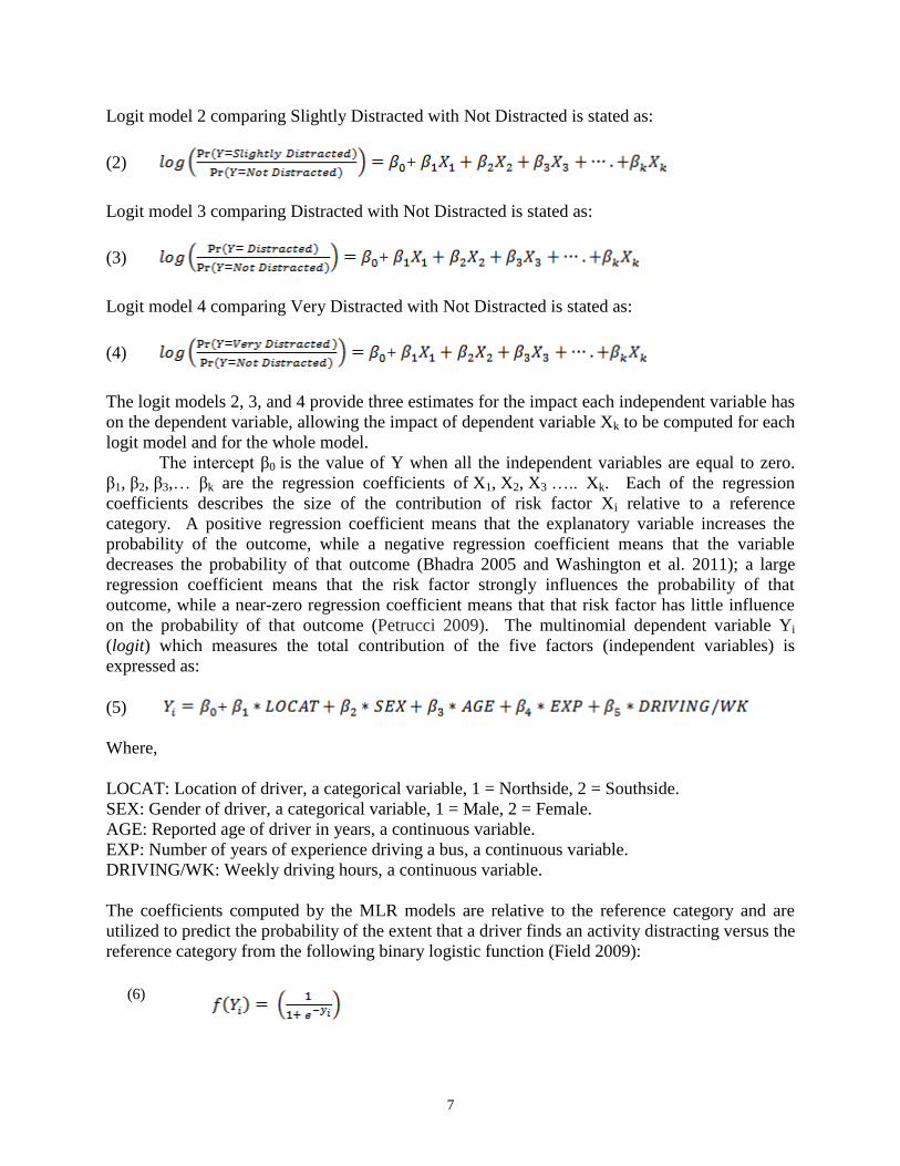
Logit model 2 comparing Slightly Distracted with Not Distracted is stated as:
(2) +
Logit model 3 comparing Distracted with Not Distracted is stated as:
(3) +
Logit model 4 comparing Very Distracted with Not Distracted is stated as:
(4) +
The logit models 2, 3, and 4 provide three estimates for the impact each independent variable has
on the dependent variable, allowing the impact of dependent variable Xk to be computed for each
logit model and for the whole model.
The intercept β0 is the value of Y when all the independent variables are equal to zero.
β1, β2, β3,… βk are the regression coefficients of X1, X2, X3 ….. Xk. Each of the regression
coefficients describes the size of the contribution of risk factor Xi relative to a reference
category. A positive regression coefficient means that the explanatory variable increases the
probability of the outcome, while a negative regression coefficient means that the variable
decreases the probability of that outcome (Bhadra 2005 and Washington et al. 2011); a large
regression coefficient means that the risk factor strongly influences the probability of that
outcome, while a near-zero regression coefficient means that that risk factor has little influence
on the probability of that outcome (Petrucci 2009). The multinomial dependent variable Yi
(logit) which measures the total contribution of the five factors (independent variables) is
expressed as:
(5) +
Where,
LOCAT: Location of driver, a categorical variable, 1 = Northside, 2 = Southside.
SEX: Gender of driver, a categorical variable, 1 = Male, 2 = Female.
AGE: Reported age of driver in years, a continuous variable.
EXP: Number of years of experience driving a bus, a continuous variable.
DRIVING/WK: Weekly driving hours, a continuous variable.
The coefficients computed by the MLR models are relative to the reference category and are
utilized to predict the probability of the extent that a driver finds an activity distracting versus the
reference category from the following binary logistic function (Field 2009):
(6)

8
Where, f (Yi) is the probability of a driver getting Slightly Distracted, Distracted, or Very
Distracted.
Each level is referenced versus Not Distracted. The event Y is very unlikely to occur if f
(Yi) is close to 0 and very likely to occur if it is close to 1. The output is split into three tables
since the dependent categorical variables are compared in pairs. Due to space restriction, the
statistical test ratios and parameter estimates for Passenger Using Mobile Phone (Risk Zone I)
has been presented in Table 5. The statistical package (SPSS 17.0 2008) includes direct entry of
all variables in the MLR model. It is not necessary to create dummy variables for categorical
variables LOCAT and SEX since the software will do this automatically when these variables are
inputted as “factors” in the software package. The analysis was conducted for each of the seven
distracting activity in the Risk Zone I, II, and III (Figure 1) to estimate the utility function Yij
(logit) of the MLR model that best fits the data for each distracting activity. Out of seven MLR
models developed for the Risk Zone activities, six were found to be highly significant and
exhibiting a good fit (Table 6). The utility function Yij (logit) for distracting levels included
independent variable coefficients that were not-significant (N/S) at the 0.05 level.
Table 5: MLR Model Outputs for Passenger Using Mobile Phone.
Model Chi-Square (χ2) =
71.56 (24)****
Pearson Stat (NS)
Deviance Stat(NS)
R2 = 0.833 (Cox &
Snell); 0.897
(Nagelkerke);
0.678(McFadden)
AIC initial/final values: 119.76/87.93
BIC initial/final values: 150.16/133.53
Independent Predictor
Variables and Interactions
Coeff β (SE)
Wald
Statistic
Odds Ratio
Exp (B)
95% CI includes
1
Slightly distracting vs. Not distracting
Intercept -105.49 (47.85)** 4.86
LOCAT = 1 -9.48 (3.05)*** 9.64 < 1 No
LOCAT = 2 0.00
SEX =1 82.41 (21.78)**** 14.31 > 1 No
SEX = 2 0.00
AGE 1.65 (0.82)** 4.01 > 1 No
EXP 2.57 (1.23)** 4.34 > 1 No
DRIVING/WK 1.89 (1.01)* 3.49 > 1 Yes
AGE*DRIVING/WK -0.03 (0.02)* 2.90 < 1 Yes
SEX=1*DRIVING/WK -1.70 (0.45)**** 14.45 < 1 No
AGE*EXP -0.04 (0.02)* 3.46 < 1 Yes
Distracting vs. Not distracting
Intercept +156.58
(51.15)***
9.37
LOCAT = 1 -5.82 (2.02)*** 8.29 < 1 No
LOCAT = 2 0.00
SEX =1 20.06 (9.68)** 4.29 > 1 No
SEX = 2 0.00
AGE -2.72 (0.88)*** 9.51 < 1 No
EXP 3.69 (1.38)*** 7.09 > 1 No
DRIVING/WK -3.79 (1.23)*** 9.54 < 1 No
AGE*DRIVING/WK 0.070 (0.02)*** 9.80 > 1 No
SEX=1*DRIVING/WK 0.36 (0.20)* 3.16 < 1 Yes
AGE*EXP -0.06 (0.02)** 6.55 < 1 Yes
Very distracting vs. Not distracting N/S
*p < 0.10; **p < 0.05; ***p < 0.01; ****p < 0.001. N/S = Not Significant.

9
MLR Model Results. The magnitude and direction of each constant term and significant
independent variable coefficient of the MLR utility functions in Table 6 along with odds ratios
were used to identify the impact of each change on the categorical dependent variable (UCLA
2007 and Washington et al. 2011). A higher or positive amount of a coefficient of the
independent variable would result in a higher dependent variable outcome and vice versa.
Where the confidence interval does not include 1.0 and odds ratio is greater than 1 indicates a
greater likelihood for a driver to get distracted versus not getting distracted by the risk zone
activity for a unit increase in the independent variable. Similarly, where the confidence interval
does not include 1.0 and odds ratio is less than 1 indicates a lower likelihood for a driver to get
distracted versus not getting distracted by the risk zone activity for a unit increase in the
independent variable.
CONSTANT TERM: The logit Y12 for Passenger Using Mobile Phone has a negative constant
term and Y13 has a positive constant term. Hence, keeping everything else the same, the driver
is less likely to get slightly distracted than distracted. The logit Y23 for Passenger has a negative
constant term. Hence, keeping everything else the same, the driver is less likely to get distracted
than slightly distracted followed by very distracted. The logit Y43 for activity Passenger Not
Following Etiquette has a positive constant term. Hence, keeping everything else the same, the
driver is more likely to get distracted than slightly distracted followed by very distracted. Some
of the logit Yij have missing constant terms resulting in rescaling of the remaining constants
(Washington et al. 2011).
Table 6: MLR Utility Functions for Risk Zone Activities.
Activity Slightly Distracting (2) Distracting (3) Very Distracting (4)
Passenger Using
Mobile Phone (1)
(Y12) = -105.49 – 9.48LOCAT +
82.41SEX+1.65AGE
+2.57EXP+1.89DRIVING/WK
(Y13) = 156.58 – 5.82LOCAT + 20.06SEX –
2.72AGE +3.67EXP – 3.79DRIVING/WK
N/S**
Passengers (2) (Y22) = – 2.20LOCAT +
16.05SEX+0.13DRIVING/WK
(Y23) = -224.35 + 235.99SEX
+0.20EXP+4.53DRIVING/WK
(Y24) =
0.47DRIVING/WK
Fatigue/Sick (3) N/S N/S (Y34) = 137.74SEX
Passenger Not
Following
Etiquette (4)
(Y42) = – 4.47LOCAT + 53.49SEX (Y43) = 323.22 – 6.52LOCAT -6.26AGE -
7.99DRIVING/WK
(Y44) = 152.61SEX
Ticket Machine
(5)
(Y52) = 1050.21 – 11.51LOCAT - 68.67SEX-
20.30AGE +23.86EXP-26.51DRIVING/WK
N/S N/S
Climate
Control(6)
(Y62) = -1.46LOCAT - 0.05DRIVING/WK N/S N/S
Passenger Trying
to Talk to Driver
(7)
Model N/S Model N/S Model N/S
Note: SPSS 17.0 sets the reference level Not Distracted = 0 with Slightly Distracting (2), Distracting (3), and Very
Distracting (4) set = 1; Peninsula = 1 and Southside = 0; Male = 1 and Female = 0.
(Yij) is the estimated utility function that measures the total contribution of each significant factor where, column i =
1 to 6, and row j = 2 to 4. N/S = MLR Final Model or individual independent variables were not significant.

10
LOCATION: The driving location had a significant impact on the level at which a driver would
find the risk zone activity distracting. The multinomial independent variable LOCAT compares
Northside driving routes to Southside driving routes for the dependent variable. Since, the
coefficient of the variable LOCAT is consistently negative and odds ratios are < 1, one could
conclude that Southside drivers are more likely to get Slightly Distracted followed by Distracted
than Northside drivers by the passenger and technology related risk zone activities. It appears
that the higher distraction could possibly lead to increased safety hazard thereby confirming
occurrence of higher accident rate in the Southside (62 accident/million miles) compared to the
Northside (54 accident/million miles).
SEX: The literature reports mixed results for the impact of gender on driver distraction. The
multinomial independent variable SEX compares male drivers to female drivers for the
dependent variable. Since, the coefficient of the variable SEX is consistently positive and odds
ratios are > 1, one could conclude that male drivers are more likely than female drivers to get
Slightly Distracted followed by Distracted and Very Distracted by any of the passenger related
activities. Other studies have shown that male truck drivers are more likely to be involved in
rear-ended crashes (possibly due to distraction) compared to female drivers (Yan, et. al. 2009).
Female drivers are more likely than male drivers to get Slightly Distracted with the Ticket
Machine.
AGE: Age is an important factor related to accidents with younger drivers more prone to
distracted driving and accidents. The average age of the regional transit bus driver is 49 years
with Southside drivers slightly older (51 years) compared to Northside drivers (47 years).
Earlier studies conducted on passenger vehicle concluded that age of a driver had a significant
impact on distraction, with younger and older drivers more prone to distraction. This study
reveals positive and negative impact of age on distraction. The coefficient of the variable AGE
for technology-related activities such as Ticket Machine is a negative value and odds ratio is < 1
indicating that as age of the driver increases, drivers are less likely to get Slightly Distracted by
the ticket machine. The coefficient of the variable AGE for passenger-related distractions are
negative (except for slightly distracted) and odds ratio < 1 indicating that as age of the driver
increased, drivers are less likely to get slightly distracted followed by distracted due to
passenger-related activities.
EXPERIENCE: The transit bus drivers had an average of 12 years experience driving buses.
There was a significance difference in driving experience in both locations with drivers on the
Southside (15 years) having more driving experience as compared to the Northside drivers (8
years). It is believed that experienced drivers would get less distracted by the distracting
activities. The coefficient of EXP variables are consistently positive values and the odds ratios
are > 1, indicating that added experience increases the likelihood of getting Slightly Distracted
followed by Distracted due to passenger and ticket machine related activities. This appears
contrary to popular belief, where experience made a driver better at handling distraction and
possibly due to the more experienced Southside drivers also has a high accident rate.
DRIVING HOURS/WEEK: The bus drivers reported that they drive a bus for an average of 43
hours per week and that they typically drive the buses mostly during the day (65%) peak and
non-peak times and during the night (35%). The driving hours per week has been found to be
related to driver error although it was not reported as driver distraction. This study finds positive
and negative impact of driving load on distraction. The coefficients of the variable
DRIVING/WEEK for technology-related distraction such as Ticket Machine and Climate
Control are negative values and odds ratios < 1 indicating that as drivers with higher driving load

11
are less likely to get slightly distracted by technology related activities. The coefficient of the
variable DRIVING/WEEK for passenger-related activities is negative and positive values, hence
no conclusions could be drawn.
MODEL ASSESSMENT AND VALIDATION OF RESULTS
The likelihood ratio test using model fitting information for Passenger Using Mobile Phone is
presented in Table 5. It shows that the difference in the -2Log Likelihood between the intercept
only (without any independent variables) and the final model (with all the independent variables)
provides the chi-square (χ2) = 71.56 (24) signifying a good improvement in the model fit. It
follows that the independent variables contribute significantly to the outcome of the distraction
level. The values of the AIC (119.76/87.93) and the BIC (150.16/133.53) gets smaller during the
stepwise process indicating a good fit for the final model. Table 5 shows the model’s Goodness
of Fit as indicated by the multiple statistics. The p values for Pearson and Deviance (both test
the same results) chi-square (χ2) = 1.00 (p = 1) proving no significance. Hence, the predicted
values of the model are not significantly different from the observed values at all outcome levels
– the model fits the data well. The measures of Pseudo R2 (0,833, 0.897, and 0.678) are
reasonably similar and high values resulting in a good fit. The impact of each coefficient is
summarized in Table 7.
Table 7: Impact of Independent Variable Coefficients on Risk Zone Activities.
High Risk
Activity
Location Sex Age Driving Exp Driving Hrs/Wk
Passenger
Using
Mobile
Southside Drivers are
more likely to get
Slightly Distracted
followed by Distracted
Male Drivers are
more likely to get
Slightly Distracted
followed by
Distracted.
Older Drivers
are more likely
to get Slightly
Distracted but
less likely to
get Distracted.
Drivers with more
driving experience
are more likely to
get Slightly
Distracted followed
by Distracted
Drivers doing more
driving hours are
more likely to get
Slightly Distracted
but less likely to get
Distracted
Passenger Southside Drivers are
more likely to get
Slightly Distracted.
Male Drivers are
more likely to get
Distracted followed
by Slightly
Distracted.
N/S Drivers having more
driving experience
are more likely to
get Distracted
Drivers doing more
driving hours are
more likely to get
Distracted followed
by Very Distracted,
or Slightly Distracted.
Fatigue/Sick N/S Male Drivers are
more likely to get
Very Distracted.
N/S N/S N/S
Passenger
Not
Following
Etiquette
Southside Drivers are
more likely to get
Slightly Distracted
followed by Distracted
Male Drivers are
more likely to get
Very Distracted
followed by Slightly
Distracted
Older Drivers
are less likely
to get
Distracted.
N/S Drivers doing more
driving hours are less
likely to get
Distracted
Ticket
Machine
Southside Drivers are
more likely to get
Slightly Distracted.
Female Drivers are
more likely to get
Slightly Distracted
Older Drivers
are less likely
to get Slightly
Distracted.
Drivers having more
driving experience
are more likely to
get Slightly
Distracted.
Drivers doing more
driving hours are less
likely to get Slightly
Distracted
Climate
Control
Southside Drivers are
more likely to get
Slightly Distracted.
N/S N/S N/S Drivers doing more
driving hours are less
likely to get Slightly
Distracted

12
The graphical methods were found suitable to assess the best fit of the binary logistic regression
model (Landwehr et al. 1984), since model inadequacies are generally reflected in the pattern of
residuals generated by the statistical package (SPSS 17.0 2008). The model’s output data was
analyzed by plotting the Pearson residuals versus the Predicted Probability. The residuals are
scattered randomly above and below the line without any pattern over the entire range of the
predicted values (Figure 2).
Figure 2: Scatter plot of Pearson residuals
The MLR models developed for the risk zone activities provide estimates of the current levels of
distraction at the transit agency. Are the results generated from the MLR models for each risk
zone activity listed in Table 7 valid for a large random population of transit bus drivers?
Simulation of the models using probabilistic distributions generates driver distraction events that
would occur in practice over a range of random factors. Monte Carlo simulation using discrete
distribution that incorporate random variability into the model was applied to validate a model’s
output results. The MLR model for each risk zone activity was repeatedly simulated by a
different random set of values (inputs) drawn from the cumulative probability distribution of the
independent variable coefficients resulting in a set of possible distraction outcomes (outputs).
Each MLR logit in Table 6 were validated for 1,000 drivers by Monte Carlo simulation. The
simulated outputs presented graphically were compared to the MLR results in Table 7.
The Simulation Spreadsheet Model
The MLR model for each risk zone activity was defined along with their probability functions.
The probability function f(Yi) represented by Equation 6, for binary logistic regression models is
applicable to MLR models by breaking down the dependent variable into a series of pair wise
comparisons between two categories (Moutinho and Hutcheson 2011 and Field 2009). Each of
the MLR utility function Yij (Table 6) for the risk zone activities was simulated for 1,000
replications (bus drivers) with randomly selected location, age, sex, driving experience, and
driving hours/week. The cumulative probability distributions for each independent variable used
by the simulation model to generate the pseudorandom numbers were developed from the survey
data.

13
Following the approach of Smith et al. (2005), the five independent variable were
simulated for 1,000 replications one at a time, keeping the remaining variables constant (Albright
and Winston 2005). For each set of 1,000 replications, the simulation spreadsheet model
generated average probability values for Yij. The impact of independent variable coefficients on
high risk activities (Table 7) were validated by comparison with the simulated outputs.
MLR Model Validation
For each risk zone activity, the simulation spreadsheet model generated average probability
values for 1,000 drivers getting Slightly Distracted, Distracted, and Very Distracted by the
impact of the factors. They are presented as follows:
LOCATION. The MLR results for the five risk zone activities in Table 8 indicates that the
Southside drivers have a higher chance of getting Slightly Distracted and Distracted versus Not
Distracted. The simulation output in Figure 3 validates these results for all the passenger-related
activities and Climate Control. In the case of Ticket Machine, the probability of getting Slightly
Distracted is the same for Southside and Northside drivers.
SEX. The MLR results for the five risk zone activities in Table 9 indicates that male drivers
have a higher chance of getting Slightly Distracted, Distracted, and Very Distracted versus Not
Distracted. The simulation output in Figure 4 validates these results for all the passenger-related
activities and Fatigue/Sickness. In the case of Ticket Machine, the probability of getting Slightly
Distracted is the same for male and female drivers.
AGE. The MLR results for the three risk zone activities in Table 10 indicates that older drivers
have a higher chance of getting Slightly Distracted but less chance of getting Distracted by
Passenger Using Mobile Phone, Passenger Not Following Etiquette, and Ticket Machine. The
simulation output in Figure 5 validates these results for all the passenger-related activities. In the
case of Ticket Machine, the probability of getting Slightly Distracted is the same for older and
younger drivers.
DRIVING EXP. The MLR results for the three risk zone activities in Table 11 indicates that
more experienced drivers have a higher chance of getting Slightly Distracted and Distracted by
Passenger-related activities and Ticket Machine. The simulation output in Figure 6 validates
these results for Passenger Using Mobile Phone. In the case of Passenger and Ticket Machine,
the probability of getting Slightly Distracted and Distracted is the same for more experienced and
less experienced drivers.
DRIVING/WEEK. The MLR results for the five risk zone activities in Table 12 indicates that
drivers with more driving hours/week have a higher chance of getting Slightly Distracted and
Distracted by Passenger Using Mobile Phone but less Distracted by Passenger Not Following
Etiquette, Ticket Machine, and Climate Control. The simulation output in Figure 7 validates
these results for Passenger Using Mobile Phone and Passenger. In the case of Passenger Not
Following Etiquette and Ticket Machine, the probability of getting Slightly Distracted and
Distracted is the same for drivers with > 40 hours/week or < 40 hours/week.

14
Table 8: MLR Results for Location Risk Zone
Activity
MLR Results – Location Simulation Results (Fig. 3)
Passenger
Using Mobile
Phone
Southside Drivers are more
likely to get Slightly
Distracted followed by
Distracted
Probability of Slightly
Distracted and Distracted is
higher for Southside Drivers
Passenger Southside Drivers are more
likely to get Slightly
Distracted.
Probability of Slightly
Distracted is higher for
Southside Drivers
Passenger Not
Following
Etiquette
Southside Drivers are more
likely to get Slightly
Distracted followed by
Distracted
Probability of Slightly
Distracted and Distracted is
higher for Southside Drivers
Ticket Machine Southside Drivers are more
likely to get Slightly
Distracted.
Probability of Slightly
Distracted Equal for both
locations
Climate Control Southside Drivers are more
likely to get Slightly
Distracted.
Probability of Slightly
Distracted is higher for
Southside Drivers
Figure 3: Simulation Results for Location.
Table 9: MLR Results for Sex Risk Zone Activity MLR Results – Sex Simulation Results (Fig.
4)
Passenger Using
Mobile Phone
Male Drivers are more
likely to get Slightly
Distracted followed by
Distracted.
Probability of Slightly
Distracted and Distracted
is higher for Male Drivers
Passenger Male Drivers are more
likely to get Distracted
followed by Slightly
Distracted.
Probability of Slightly
Distracted and Distracted
is higher for Male Drivers
Fatigue/Sick Male Drivers are more
likely to get Very
Distracted.
Probability of Very
Distracted is higher for
Male Drivers
Passenger Not
Following Etiquette
Male Drivers are more
likely to get Very
Distracted followed by
Slightly Distracted
Probability of Slightly
Distracted and Very
Distracted is higher for
Male Drivers
Ticket Machine Female Drivers are more
likely to get Slightly
Distracted
Probability of Slightly
Distracted Equal for both
locations
Figure 4: Simulation Results for Sex

15
Table 10: MLR Results for Age Risk Zone Activity MLR Results – Age Simulation Results
(Fig. 5)
Passenger Using
Mobile Phone
Older Drivers are
more likely to get
Slightly Distracted
but less likely to get
Distracted.
Probability of Slightly
Distracted increases
with age and
Probability of
Distracted reduces
with age
Passenger Not
Following Etiquette
Older Drivers are less
likely to get
Distracted.
Probability of
Distracted reduces for
older drivers
Ticket Machine Older Drivers are less
likely to get Slightly
Distracted.
Probability of Slightly
Distracted Equal for
all ages
Figure 5: Simulation Results for Age.
Table 11: MLR Results for Driving Experience Risk Zone
Activity
MLR Results – Driving
Exp
Simulation Results (Fig. 6)
Passenger Using
Mobile Phone
Drivers with more driving
experience are more likely
to get Slightly Distracted
followed by Distracted
Probability of Slightly
Distracted and Distracted
increases with Driving
Experience
Passenger Drivers having more
driving experience are
more likely to get
Distracted
Probability of Distracted
Equal for all driving
experience
Ticket Machine Drivers having more
driving experience are
more likely to get Slightly
Distracted.
Probability of Slightly
Distracted Equal for all
driving experience
Figure 6: Simulation Results for Driving Experience
16
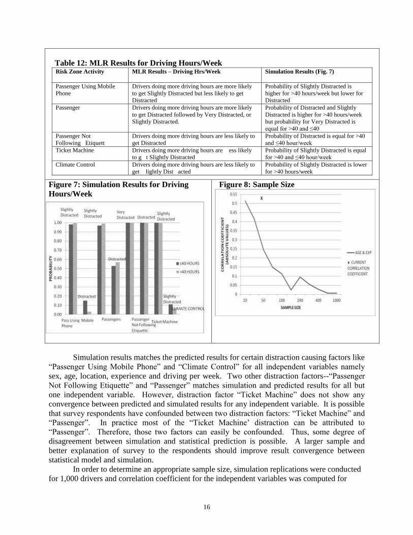
Table 12: MLR Results for Driving Hours/Week Risk Zone Activity MLR Results – Driving Hrs/Week Simulation Results (Fig. 7)
Passenger Using Mobile
Phone
Drivers doing more driving hours are more likely
to get Slightly Distracted but less likely to get
Distracted
Probability of Slightly Distracted is
higher for >40 hours/week but lower for
Distracted
Passenger Drivers doing more driving hours are more likely
to get Distracted followed by Very Distracted, or
Slightly Distracted.
Probability of Distracted and Slightly
Distracted is higher for >40 hours/week
but probability for Very Distracted is
equal for >40 and ≤40
Passenger Not
Following Etiquett
Drivers doing more driving hours are less likely to
get Distracted
Probability of Distracted is equal for >40
and ≤40 hour/week
Ticket Machine Drivers doing more driving hours are ess likely
to g t Slightly Distracted
Probability of Slightly Distracted is equal
for >40 and ≤40 hour/week
Climate Control Drivers doing more driving hours are less likely to
get lightly Dist acted
Probability of Slightly Distracted is lower
for >40 hours/week
Figure 7: Simulation Results for Driving
Hours/Week
Figure 8: Sample Size
Simulation results matches the predicted results for certain distraction causing factors like
“Passenger Using Mobile Phone” and “Climate Control” for all independent variables namely
sex, age, location, experience and driving per week. Two other distraction factors--“Passenger
Not Following Etiquette” and “Passenger” matches simulation and predicted results for all but
one independent variable. However, distraction factor “Ticket Machine” does not show any
convergence between predicted and simulated results for any independent variable. It is possible
that survey respondents have confounded between two distraction factors: “Ticket Machine” and
“Passenger”. In practice most of the “Ticket Machine’ distraction can be attributed to
“Passenger”. Therefore, those two factors can easily be confounded. Thus, some degree of
disagreement between simulation and statistical prediction is possible. A larger sample and
better explanation of survey to the respondents should improve result convergence between
statistical model and simulation.
In order to determine an appropriate sample size, simulation replications were conducted
for 1,000 drivers and correlation coefficient for the independent variables was computed for

17
various sample sizes. The current sample size of 48 results in a high correlation coefficient of
0.54 for variables Age and Experience. The correlation coefficient reduces as the sample size is
increased (Figure 8). A larger sample size would result in low standard error; and will be above
the preferred a case-to-variable ratio of 20:1 recommended by researchers (Petrucci 2009).
CONCLUSION
The results of the MLR models indicate that passenger-related activities which are beyond the
control of the driver are most distracting to the driver. It is therefore a challenge for the transit
agency to develop effective policies for handling passenger behavior, so that they are less likely
to engage in using cell phones, non etiquette behavior, noisy behavior etc. For example,
personal electronic devices could be allowed to be used beyond the middle section of the bus to
avoid distracting the driver. The front section of the bus could be designated as cell phone free.
Drivers must avoid unnecessary communications with passengers and if conversation cannot be
avoided, it must be done with caution while concentrating on the road ahead, or when the bus is
stopped. Training should focus on male drivers who are more likely to get distracted by
passengers.
Educational training program on the proper use of technological devices mounted in the
cab or issued to the driver, and hazards associated with utilizing these devices while driving
should focus on older and female drivers who are likely to get distracted with technological
devices. The design of ticket machine, control panel, and other devices must be user-friendly,
and not require long glances away from the forward roadway.
How could the transit agency use the MLR models developed in this study? They could
be applied to predict distraction for varying driver characteristics and driving patterns. It is
observed that drivers with differing factors are affected differently by distracting activities which
may be possibly corrected through proper training. The transit agency could develop driver
MLR models for each risk zone activity from its existing driver database. These models could be
used for predicting the probability of a new driver getting distracted by the risk zone activities. If
the probability value is high, the new driver could be scheduled for related training. Other
transit agencies could use this study as a framework for distraction analysis of their drivers.
The relatively small number of surveys completed (48 drivers) out of a total of 265
surveys distributed to bus drivers’ results in a low response rate of 18%. This amounts to a
number of cases per independent variable of 9.6 which is below the preferred a case-to-variable
ratio of 20:1. In addition to the five independent variables, other variables such as
environmental, vehicle, roadway designs etc could also have an impact on driver distraction but
have not been included in the MLR model. (Washington et al. 2011; Morfoulaki et al. 2007; Yan
et al. 2009; Gkritza et al. 2006). The classification of risk zone activities is somewhat subjective
and could be replaced by an objective index system similar to the Hazard Index developed by
Smith et al. (2005).
The presence of Multicollinearity that was detected from the Pearson Correlation analysis
makes it difficult to determine the relative importance of each independent variable on the
regression model and the effects on the dependent variable (Washington et al. 2011).
Furthermore, there may be curvilinear relationship between age and driving experience, resulting
in the violation of the linear assumption. There is no strong evidence at this point in the analysis
for adding or deleting any of the interactions. The increase in sample size (Figure 8) may reduce
the standard error, thereby mitigating the threat of multicollinearity. Furthermore, the MLR data

18
was not tested to show it meets the Independence of Irrelevant Alternative (IIA) specifications
which require the ratio of probabilities of selecting any two alternatives to be independent of the
third choice (Small and Hsiao 1985).
This exploratory study is one of only a few to examine the full range of distractions and
associated risk in transit buses. It has limited applications due to localized sample size and
limitations discussed above; hence inferences may not be drawn for the larger population of bus
drivers in the Commonwealth of Virginia or the United States. It should be followed by an
expanded study covering a larger sample of drivers form other agencies. Knowing the activities
that cause a high risk of distraction as well as the related factors may provide additional inputs to
law and policy makers while crafting legislations and regulations statewide or nationwide.
REFERENCES
AAA Foundation for Traffic Safety. “Distraction in Everyday Driving.” University of North
Carolina at Chapel Hill, Highway Safety Research Center, June, 2003. www.aaafoundation.org.
Albright, S. C, and W. L. Winston. “Introduction to Simulation Modeling.” Spreadsheet
Modeling and Applications: Essentials of Practical Management Science. Thomson
Brooks/Cole (2005): 423 – 488.
Bhadra, Dipasis. “Choice of Aircraft Fleets in the U. S. Domestic Scheduled Air Transportation
System: Findings from a Multinomial Logit Analysis.” Journal of the Transportation Research
Forum 44 (3), (2005): 143 – 162.
Blower, D., P. E. Green, and A. Matteson. “Bus Operator Types and Driver Factors in Fatal Bus
Crashes: Results from the Buses Involved in Fatal Accidents Survey.” U. S. DOT Federal Motor
Carrier Safety Administration. University of Michigan Transportation Research Institute, Ann
Arbor Michigan, June, 2008.
Bonate, Peter L. “A Brief Introduction to Monte Carlo Simulation.” Clin Pharmacokinetics 40
(1), (2001): 15-22.
Carlson, William L. “Application of Simulation to Assessment of Component Changes on rear
End Highway Accidents.” Transportation Science 6 (1), (February, 1972): 1 – 14.
Cross, G. W., H. Hanna, T. Garrison, and C. McKee. “Distracted Driving in Mississippi: A
Statewide Survey and Summary of Related Research and Policies.” Final Report by Family and
Children Research Unit, MSU. The Center for Mississippi Health Policy, September, 2010.
Daily Press Newspaper. “In States Across U. S. New Traffic Laws Gain Traction.” Nation &
World, January 02, 2012.
D’Souza, K. A. and S. K. Maheshwari. “Improving Performance of Public Transit Buses by
Minimizing Driver Distraction.” Urban Transport 2012 Conference, Coruňa, Spain,
(forthcoming) May 13-16, 2012.

19
Field, Andy. “Logistic Regression.” Discovering Statistics Using SPSS. SAGE Publications
Ltd., 3rd
Edition, (2009): 264 - 315.
Gkritza, K., D. Niemeier, and F. Mannering. “Airport Security Screening and Changing
Passenger Satisfaction: An Exploratory Assessment.” Journal of Air Transport Management 12,
(2006): 213 – 219.
Hickman, J. S., R. J. Hanowski, and J. Bocanegra. “Distraction in Commercial Trucks and
Buses: Assessing Prevalence and Risk in Conjunction with Crashes and Near-Crashes.” U.S.
DOT, Federal Motor Carrier Safety Administration, Office of Analysis, Research and
Technology, Washington, D.C., September, 2010.
Landwehr, J. M., D. Pregibon, and A. C. Shoemaker. “Graphical Methods for Assessing
Logistic Regression Models.” Journal of the American Statistical Association 79(385), (March,
1984): 61 – 71.
Metro Magazine. “Study: Transit Drivers Involved in Collisions Twice as Likely to Use Phone
While Driving.” Industry News. January 18, 2011.
Morfoulaki, M., Y. Tyrinopoulos, and G. Aifadopoulou. “Estimation of Satisfied Customers in
Public Transport Systems: A New Methodological Approach.” Journal of the Transportation
Research Forum 46(1), (Spring, 2007): 63-72.
Moutinho, L., and G. Hutcheson. “Multinomial Logistic Regression.” The SAGE Dictionary of
Quantitative Management Research. SAGE Publications Ltd. (2011): 208 -212.
Owens, J. M., and R. Lehman. “The Effects Of Age And Distraction On Reaction Time In A
Driving Simulator.” 1st International Driving Symposium on Human Factors in Driver
Assessment, Training and Vehicle Design, Aspen, CO, August 14 – 17, (2001): 147-152.
Oxley, J., J. Charlton, B. Fildes, S. Koppel, J. Scully, M. Congiu, and K. Moore. “Crash Risk of
Older Female Drivers.” Report No. 245. Monash University Accident Research Center,
Victoria, Australia, November, 2005.
Petrucci, Carrie J. “A Primer for Social Worker Researchers on How to Conduct a Multinomial
Logistic Regression. Journal of Social Service Research 35(2), (2009): 193 – 205.
Salmon, P. M., K. L. Young, and M. A. Regan. “Distraction ‘On the Buses’: A Novel
Framework of Ergonomics Methods for Identifying Sources and Effects of Bus Driver
Distraction.” Applied Ergonomics 42, (2011): 602-610.
Salmon, P.M., K. L. Young, and M. A. Regan. “Bus Driver Distraction Stage 1: Analysis of
Risk for State Transit Authority New South Wales Bus Drivers..” Final Report. Monash
University Accident Research Center, Victoria, Australia, June, 2006.

20
Salvucci, D. D., A. K. Chavez, and F. J. Lee. “Modeling Effects of Age in Complex Tasks: A
Case Study in Driving.” 26th
Annual Conference of the Cognitive Science Society, 2004.
Small, K. A. and Hsiao, C. “Multinomial Logit Specification Tests.” International Economic
Review 26 (3), (October, 1985): 619-627.
Smith, D. I., J. Chang, D. Cohen, J. Foley, and R. Glassco. “A Simulation Approach for
Evaluating the Relative Safety Impact of Driver Distraction During Secondary Tasks.” 12th
World Congress on ITS, San Francisco, 6 – 10 November, (2005): Paper 4340.
SPSS 17.0. SPSS Inc., Chicago, IL 60606-6412, 2008.
UCLA Annotated SPSS Output. “Multinomial Logistic Regression.” Academic Technology
Services, Statistical Consulting Group. http://www.ats.ucla.edu/stat/sas/notes2/ , 2007.
U. S. Department of Transportation. “An Examination of Driver Distraction as Recorded in
NHSTA Databases.” DOT HS 811 216, September 2009.
U. S. Department of Transportation. “Highway Accident Report: Gray Summit, MO Collision
Involving Two School Buses, a Bobtail, and a Passenger Vehicle, August 5, 2010.” National
Transportation Safety Board, http://www.ntsb.gov/news/events/2011/gray_summit_mo, 2011.
U. S. Department of Transportation. “Statistics and Facts About Distracted Driving.”
www.distraction.gov/stats-and-facts, 2010.
Virginia Department of Motor Vehicle. “Virginia Traffic Crash Facts.” Virginia Crashes
Involving Buses. Virginia Highway Safety Office, (2008): 58.
Washington, S. P., M. G. Karlaftis, and F. L. Mannering. “Logistic Regression, Discrete
Outcome Models and Ordered Probability Models.” Statistical and Econometric Methods for
Transportation Data Analysis. Chapman & Hall/CRC, (2011): 303 - 359.
Yan, X., E. Radwan, and M. Abdel–Aty. “Characteristics of Rear-End Accidents at Signalized
Intersections Using Multiple Logistic Regression Model.” Accident Analysis and Prevention 37,
(2005): 983-995.
Yan, X., E. Radwan, and K. K. Mannila. “Analysis of Truck-Involved Rear-End Crashes Using
Multinomial Logistic Regression.” Advances in Transportation Studies an International Journal
Section A 17, (2009): 39 – 52.
Yang, C. Y. D. “Trends in Transit Bus Accidents and Promising Collision Countermeasures.”
Journal of Public Transportation 10(3), (2007): 119 – 136.


![Improving performance of public transit buses by minimizing … · 2014. 5. 13. · 2005, transit buses accounted for one third fatal crashes among all bus types [6]. In the case](https://cdn.vdocuments.net/doc/165x107/601c08c282934163663cb9cb/improving-performance-of-public-transit-buses-by-minimizing-2014-5-13-2005.jpg)
