An Immersed Boundary Method forSuspensions of Rigid Bodies
Aleksandar Donev, CIMS&
Bakytzhan Kallemov and Florencio Balboa Usabiaga, CIMSBoyce Griffith and Amneet Bhalla, UNC
Courant Institute, New York University
Numerical Analysis SeminarDec 5th 2014
A. Donev (CIMS) RigidIBM 12/2014 1 / 42
Introduction
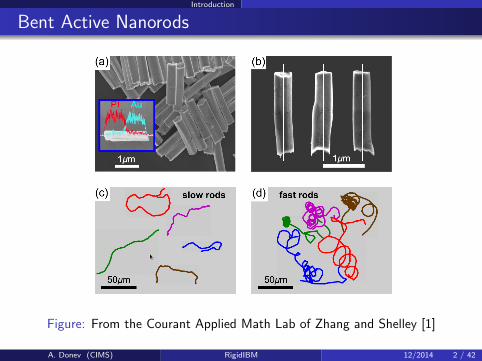
Bent Active Nanorods
Figure: From the Courant Applied Math Lab of Zhang and Shelley [1]
A. Donev (CIMS) RigidIBM 12/2014 2 / 42
Introduction
Thermal Fluctuation Flips
QuickTime
A. Donev (CIMS) RigidIBM 12/2014 3 / 42
Introduction
Steady Stokes Flow (Re→ 0)
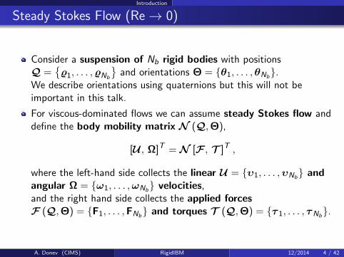
Consider a suspension of Nb rigid bodies with positionsQ =
%1, . . . ,%Nb
and orientations Θ = θ1, . . . ,θNb
.We describe orientations using quaternions but this will not beimportant in this talk.
For viscous-dominated flows we can assume steady Stokes flow anddefine the body mobility matrix N (Q,Θ),
[U , Ω]T = N [F , T ]T ,
where the left-hand side collects the linear U = υ1, . . . ,υNb and
angular Ω = ω1, . . . ,ωNb velocities,
and the right hand side collects the applied forcesF (Q,Θ) = F1, . . . ,FNb
and torques T (Q,Θ) = τ 1, . . . , τNb.
A. Donev (CIMS) RigidIBM 12/2014 4 / 42

Introduction
Brownian Motion
The Brownian dynamics of the rigid bodies is given by theoverdamped Langevin equation[
dQ/dtdΘ/dt
]=
[UΩ
]= N
[FT
]+ (2kBTN )
12 W (t) .
How to compute (the action of) N and N12 and simulate the
Brownian motion of the bodies?
This talk focuses on the deterministic aspects of computing N andnot on the stochastic aspects; but it all works together!
We will also focus on passive rigid bodies but activity in the form ofactive slip or active kinematics can easily be incorporated.
A. Donev (CIMS) RigidIBM 12/2014 5 / 42
Introduction
Goals / Preview
Our methods are unique in that they:
Work for the steady Stokes regime (Re = 0) as well as finiteReynolds numbers because there is no time splitting.
Strictly enforce the rigidity constraint: no penalty parameters.
Require no Green’s functions, but rather, use a finite-volumestaggered-grid fluid solver to include hydrodynamics.
Ensure fluctuation-dissipation balance even in the presence ofnontrivial boundary conditions.
A. Donev (CIMS) RigidIBM 12/2014 6 / 42

Semi-continuum rigid-body formulation
Immersed Rigid Body
In the immersed boundary method we extend the fluid velocityeverywhere in the domain,
ρ∂tv + ∇π = η∇2v +
∫Ωλ (q) δ (r − q) dq + ∇ ·
(√2ηkBT W
)∇ · v = 0 everywhere
me u = F−∫
Ωλ (q) dq
Ieω = τ −∫
Ω
[(q− %0
)× λ (q)
]dq
v (q, t) = υ +(q− %0
)× ω for all q ∈ Ω
=
∫v (r, t) δ (r − q) dr,
where the induced fluid-body force [2] λ (q) is a Lagrangemultiplier enforcing the final no-slip condition (rigidity).
A. Donev (CIMS) RigidIBM 12/2014 7 / 42
Semi-continuum rigid-body formulation
Immersed-Boundary Method
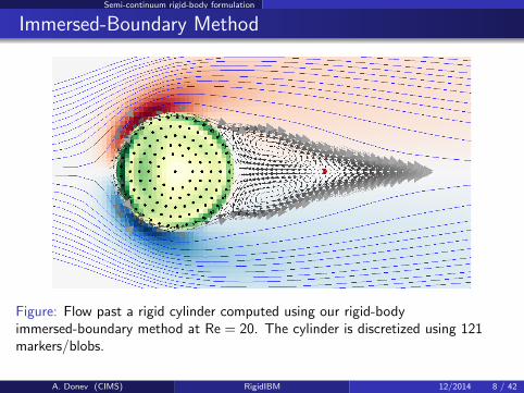
Figure: Flow past a rigid cylinder computed using our rigid-bodyimmersed-boundary method at Re = 20. The cylinder is discretized using 121markers/blobs.
A. Donev (CIMS) RigidIBM 12/2014 8 / 42

Semi-continuum rigid-body formulation
Blob/Bead Models
Figure: Blob or “raspberry”models of: a spherical colloid, and a lysozyme [3].
The rigid body is discretized through a number of “markers” or“blobs” [4] with positions Q = q1, . . . ,qN.Composite velocity U = u1, . . . ,uN and rigidity forcesΛ = λ1, . . . ,λN.
A. Donev (CIMS) RigidIBM 12/2014 9 / 42

Semi-continuum rigid-body formulation
Blob Model
Take an Immersed Boundary Method (IBM) approach and describethe fluid-blob interaction using a localized smooth kernel δa(r) withcompact support of size a (regularized delta function).
Define composite local averaging linear operator J (Q) operator, isthe composite spreading linear operator, S (Q) = J ? (Q),
ui = (J v)i = Jiv =
∫δa (qi − r) v (r, t) dr
λ (r) = (SΛ) (r) =N∑i=1
λiδa (qi − r) =N∑i=1
Siλi .
In reality these are sums over grid points and δa is the Peskin 6-ptkernel.
A. Donev (CIMS) RigidIBM 12/2014 10 / 42
Semi-continuum rigid-body formulation
Rigid-Body Immersed-Boundary Method
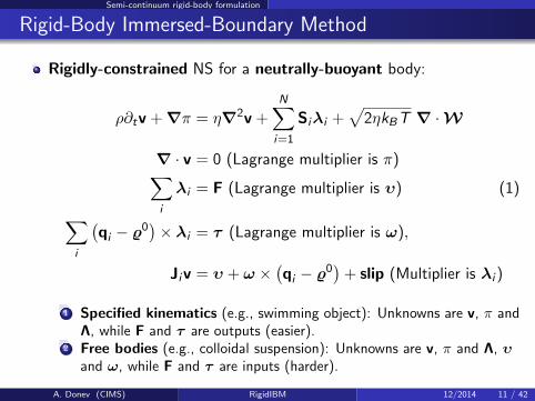
Rigidly-constrained NS for a neutrally-buoyant body:
ρ∂tv + ∇π = η∇2v +N∑i=1
Siλi +√
2ηkBT ∇ ·W
∇ · v = 0 (Lagrange multiplier is π)∑i
λi = F (Lagrange multiplier is υ) (1)∑i
(qi − %0
)× λi = τ (Lagrange multiplier is ω),
Jiv = υ + ω ×(qi − %0
)+ slip (Multiplier is λi )
1 Specified kinematics (e.g., swimming object): Unknowns are v, π andΛ, while F and τ are outputs (easier).
2 Free bodies (e.g., colloidal suspension): Unknowns are v, π and Λ, υand ω, while F and τ are inputs (harder).
A. Donev (CIMS) RigidIBM 12/2014 11 / 42

Spatio-Temporal Discretization
Fluid Solver
Discretize the fluid equation using the staggered-grid (MAC)second-order scheme on a uniform Cartesian grid with grid spacing h,using the discrete gradient G, the discrete divergence D = −G?, andthe velocity Laplacian L.
After temporal discretization of the fluid equations, using backwardEuler or Crank-Nicolson, we get
ρ
∆tI− ηLv
Denote β = ν∆t/h2 = η∆t/(ρh2)
is the viscous CFL number,β →∞ for Steady stokes, β = 0 for inviscid, and define
A = ηh−2(β−1I− h2L
).
The dimensionless matrix β−1I− h2L is essentially a discretization ofan imaginary Helmholtz or screened Poisson equation and theaction of A−1 can be obtained using geometric multigrid.
A. Donev (CIMS) RigidIBM 12/2014 12 / 42

Spatio-Temporal Discretization
Saddle-Point Problem
Define the geometric matrix K that converts body kinematics tomarker kinematics,
KY = K [U ,Ω]T = U + Ω×(Q−Q0
).
After temporal discretization of the constrained NS equations, we getthe free-kinematics constrained Stokes saddle-point problem,
A G −S 0−D 0 0 0−J 0 0 K
0 0 K? 0
vπΛY
=
g00R
,where Y = [U , Ω]T and R = [F , T ]T , and recall that S = J ?.
A. Donev (CIMS) RigidIBM 12/2014 13 / 42
Spatio-Temporal Discretization
Fluid Solver
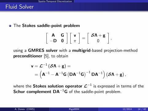
The Stokes saddle-point problem[A G−D 0
] [vπ
]=
[SΛ + g
0
],
using a GMRES solver with a multigrid-based projection-methodpreconditioner [5], to obtain
v = L−1 (SΛ + g) =
=(
A−1 − A−1G(DA−1G
)−1DA−1
)(SΛ + g) ,
where the Stokes solution operator L−1 is expressed in terms of theSchur complement DA−1G of the saddle-point problem.
A. Donev (CIMS) RigidIBM 12/2014 14 / 42
Spatio-Temporal Discretization
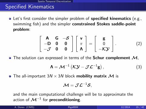
Specified Kinematics
Let’s first consider the simpler problem of specified kinematics (e.g.,swimming fish) and the simpler constrained Stokes saddle-pointproblem: A G −S
−D 0 0−J 0 0
vπΛ
=
g0−KY
. (2)
The solution can expressed in terms of the Schur complement M,
Λ = M−1(KY −JL−1g
), (3)
The all-important 3N × 3N block mobility matrix M is
M = JL−1S,
and the main computational challenge will be to approximate theaction of M−1 for preconditioning.
A. Donev (CIMS) RigidIBM 12/2014 15 / 42
Spatio-Temporal Discretization
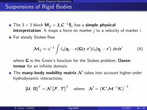
Suspensions of Rigid Bodies
The 3× 3 block Mij = JiL−1Sj has a simple physicalinterpretation: It maps a force on marker j to a velocity of marker i .
For steady Stokes flow
Mij ≈ η−1
∫δa(qi − r)G(r, r′)δa(qj − r′) drdr′ (4)
where G is the Green’s function for the Stokes problem; Oseentensor for an infinite domain.
The many-body mobility matrix N takes into account higher-orderhydrodynamic interactions,
[U , Ω]T = N [F , T ]T where N =(K?M−1K
)−1.
A. Donev (CIMS) RigidIBM 12/2014 16 / 42

Spatio-Temporal Discretization
Brownian Motion
By adding the stochastic forcing ∇ ·(√
2ηkBT W)
to the fluidequation we obtain the correct fluctuating velocities (Brownianmotion), [
UΩ
]= N
[FT
]+ (2kBTN )
12 W ,
where the “square root” of the mobility is explicitly constructed as
N12 =
√2kBT NKM−1JL−1DvW .
Observe that discrete fluctuation-dissipation balance isguaranteed,
N12
(N
12
)?= NKM−1
(JL−1LL−1S
)M−1K?N ,
= N(KM−1K
)N = N .
This works for confined systems, non-spherical particles, and evenactive particles. Can also be extended to semi-rigid structures(e.g., bead-link polymer chains).
A. Donev (CIMS) RigidIBM 12/2014 17 / 42
Preconditioning
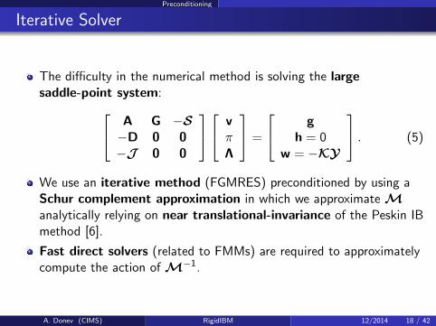
Iterative Solver
The difficulty in the numerical method is solving the largesaddle-point system: A G −S
−D 0 0−J 0 0
vπΛ
=
gh = 0
w = −KY
. (5)
We use an iterative method (FGMRES) preconditioned by using aSchur complement approximation in which we approximate Manalytically relying on near translational-invariance of the Peskin IBmethod [6].
Fast direct solvers (related to FMMs) are required to approximatelycompute the action of M−1.
A. Donev (CIMS) RigidIBM 12/2014 18 / 42
Preconditioning
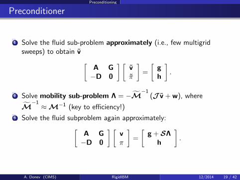
Preconditioner
1 Solve the fluid sub-problem approximately (i.e., few multigridsweeps) to obtain v [
A G−D 0
] [vπ
]=
[gh
].
2 Solve mobility sub-problem Λ = −M−1
(J v + w), where
M−1≈M−1 (key to efficiency!)
3 Solve the fluid subproblem again approximately:[A G−D 0
] [vπ
]=
[g + SΛ
h
].
A. Donev (CIMS) RigidIBM 12/2014 19 / 42

Preconditioning
Well-Posedness
The constrained Stokes system will be well-conditioned if the mobilitymatrix M has a controlled conditioning number.
We find that M is ill-conditioned if markers come closerthan two grid cells apart.
This is not unexpected at all but it is different from usual IB wisdomfor elastic bodies (markers half a grid cell apart).
If markers are too far apart the flow “leaks” through the body.
So for now we keep markers two grid cells apart and refine bothfluid grid and marker grid in unison.This should ensure a sort of LBB-like condition (?).
We can do better if we combine with a finite-element method for therigid body (see Outlook section)...
A. Donev (CIMS) RigidIBM 12/2014 20 / 42

Preconditioning
Spectrum of M
0 0.1 0.2 0.3 0.4 0.5 0.6 0.7 0.8 0.9 1
Eigenvalue rank
1×10⁻⁷
1×10⁻⁶
1×10⁻⁵
1×10⁻⁴
1×10⁻³
1×10⁻²
1×10⁻¹
1×100
Eig
enval
ue
N=42 (h=0.5)
N=162N=642N=2562N=42 (h=1.0)
N=42 (h=0.75)
Spherical shells (marker distance = 1)solid h=0.5, dash-dotted h=0.75, dashed h=1.0
A. Donev (CIMS) RigidIBM 12/2014 21 / 42
Preconditioning
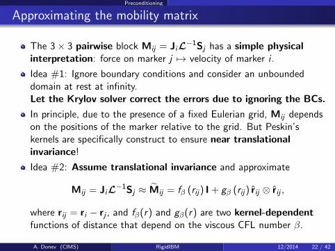
Approximating the mobility matrix
The 3× 3 pairwise block Mij = JiL−1Sj has a simple physicalinterpretation: force on marker j 7→ velocity of marker i .
Idea #1: Ignore boundary conditions and consider an unboundeddomain at rest at infinity.Let the Krylov solver correct the errors due to ignoring the BCs.
In principle, due to the presence of a fixed Eulerian grid, Mij dependson the positions of the marker relative to the grid. But Peskin’skernels are specifically construct to ensure near translationalinvariance!
Idea #2: Assume translational invariance and approximate
Mij = JiL−1Sj ≈ Mij = fβ (rij) I + gβ (rij) rij ⊗ rij ,
where rij = ri − rj , and fβ(r) and gβ(r) are two kernel-dependentfunctions of distance that depend on the viscous CFL number β.
A. Donev (CIMS) RigidIBM 12/2014 22 / 42
Preconditioning
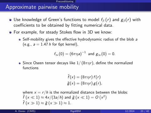
Approximate pairwise mobility
Use knowledge of Green’s functions to model fβ (r) and gβ(r) withcoefficients to be obtained by fitting numerical data.
For example, for steady Stokes flow in 3D we know:
Self-mobility gives the effective hydrodynamic radius of the blob a(e.g., a = 1.47 h for 6pt kernel),
f∞(0) = (6πηa)−1 and g∞(0) = 0.
Since Oseen tensor decays like 1/ (8πηr), define the normalizedfunctions
f (x) = (8πηr) f (r)
g(x) = (8πηr) g(r),
where x = r/h is the normalized distance between the blobs:f (x 1) ≈ 4x/(3a/h) and g (x 1) = O
(x2)
f (x 1) ≈ g (x 1) ≈ 1.
A. Donev (CIMS) RigidIBM 12/2014 23 / 42

Preconditioning
Rotne-Prager-Yamakawa Mobility
The numerical data is well-fitted by the well-knownRotne-Prager-Yamakawa tensor commonly used in Brownian dynamicssimulations:
f (r) =1
6πηa
3a4r + a3
2r3 , r > 2a
1− 9r32a , r ≤ 2a
(6)
and
g(r) =1
6πηa
3a4r −
3a3
2r3 , r > 2a3r
32a , r ≤ 2a(7)
An important property of the RPY mobility is that M is guaranteed to besymmetric positive semidefinite.
A. Donev (CIMS) RigidIBM 12/2014 24 / 42
Preconditioning
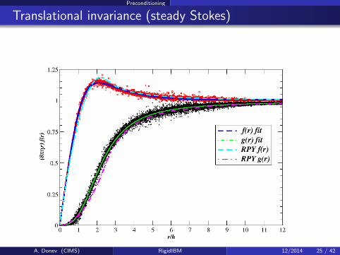
Translational invariance (steady Stokes)
A. Donev (CIMS) RigidIBM 12/2014 25 / 42
Preconditioning
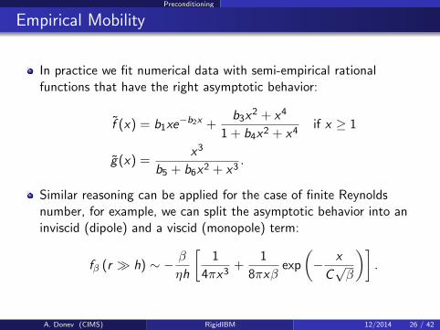
Empirical Mobility
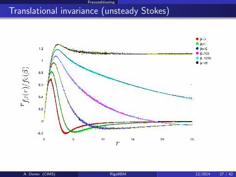
In practice we fit numerical data with semi-empirical rationalfunctions that have the right asymptotic behavior:
f (x) = b1xe−b2x +
b3x2 + x4
1 + b4x2 + x4if x ≥ 1
g(x) =x3
b5 + b6x2 + x3.
Similar reasoning can be applied for the case of finite Reynoldsnumber, for example, we can split the asymptotic behavior into aninviscid (dipole) and a viscid (monopole) term:
fβ (r h) ∼ − β
ηh
[1
4πx3+
1
8πxβexp
(− x
C√β
)].
A. Donev (CIMS) RigidIBM 12/2014 26 / 42
Preconditioning
Translational invariance (unsteady Stokes)
A. Donev (CIMS) RigidIBM 12/2014 27 / 42

Preconditioning
Fast Solvers
After we approximate M analytically, we still need to solve the linearsystem approximately
MΛ = U.
For smallish number of markers we just use dense direct linearsolvers (LAPACK). For large number of markers we needapplication-specific approaches.
We have also had some success with the HODLR low-rankapproximation fast solvers of Sivaram Ambikasaran (CIMS).
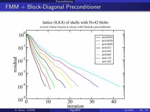
An alternative is to use an iterative solver with Fast MultipoleMethod (we are using Leslie Greengard’s codes) for the matrixvector-product, and a body-block-diagonal preconditioner (onedense diagonal block per rigid body).
Presently working with the group of Eric Darve (Stanford) to developbetter low-rank (HODLR) approximate factorizations to be used as apreconditioner for the FMM-based iterative solver...
A. Donev (CIMS) RigidIBM 12/2014 28 / 42
Preconditioning
FMM + Block-Diagonal Preconditioner
0 10 20 30 40iteration
10-5
10-4
10-3
10-2
10-1
100
resi
dual
φ=0.0010
φ=0.0029
φ=0.0089
φ=0.023
φ=0.044
φ=0.065
φ=0.125
φ=0.185
lattice (8,8,8) of shells with N=42 blobsseveral volume fraction φ, always with Cholesky-preconditioner
A. Donev (CIMS) RigidIBM 12/2014 29 / 42
Numerical Tests
Convergence
We have implemented this method using the IBAMR softwareframework developed by Boyce Griffith: RigidIBAMR.
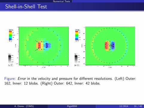
We have tested the solver on some examples of zero and finiteReynolds number flows in 2D and 3D for which analytical answers areknown, e.g., a moving sphere inside a stationary fixed shell(shell-in-shell or sphere-in-shell test) for steady Stokes.
We observe strong convergence of the force density on the surfaceof the inner sphere as we refine the grid but the convergence is onlyfirst-order (as expected) and quite slow, and very sensitive to themarker spacing due to ill-conditioning.
It appears weak convergence (of stress moments) is much morerobust and rapid: most important for suspensions and obtainingqualitatively correct physics for minimally-resolved orcoarsely-resolved models.
A. Donev (CIMS) RigidIBM 12/2014 30 / 42
Numerical Tests
Shell-in-Shell Test
Figure: Error in the velocity and pressure for different resolutions. (Left) Outer:162, Inner: 12 blobs. (Right) Outer: 642, Inner: 42 blobs.
A. Donev (CIMS) RigidIBM 12/2014 31 / 42

Numerical Tests
Steady Stokes Test
Figure: Error in the velocity and pressure for different resolutions. (Left) Outer:2562, Inner: 162 blobs. (Right) Outer: 10242, Inner: 642 blobs.
A. Donev (CIMS) RigidIBM 12/2014 32 / 42
Numerical Tests
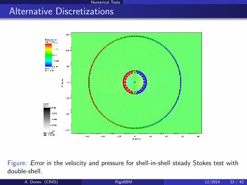
Alternative Discretizations
Figure: Error in the velocity and pressure for shell-in-shell steady Stokes test withdouble-shell.
A. Donev (CIMS) RigidIBM 12/2014 33 / 42
Numerical Tests
Strong Accuracy
0 0.5 1 1.5 2 2.5 3−0.5
0
0.5
θ
σn
10242−642 h=0.52562−162 h=1642−42 h=2theory
0 0.5 1 1.5 2 2.5 3
−0.8
−0.6
−0.4
−0.2
0
θ
σθ
10242−642 h=0.52562−162 h=1642−42 h=2theory
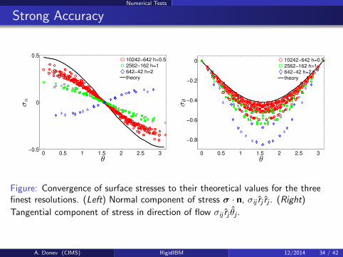
Figure: Convergence of surface stresses to their theoretical values for the threefinest resolutions. (Left) Normal component of stress σ · n, σij rj rj . (Right)
Tangential component of stress in direction of flow σij rj θj .
A. Donev (CIMS) RigidIBM 12/2014 34 / 42
Numerical Tests
Sphere in Shear Flow
The low-order moments of the fluid-particle stress convergerelatively rapidly.
The total drag (zeroth moment) and torque (antisymmetric part ofthe second moment),
F =∑i
Λi and τ =∑i
λi × ri .
These are nonzero and consistent even for a single blob.
But to get a nonzero stresslet (symmetric part of the secondmoment) we need a raspberry-type model,
S = SymmTraceless
∑i
λi ⊗ ri
.
A. Donev (CIMS) RigidIBM 12/2014 35 / 42

Numerical Tests
Weak Accuracy
Compare to theoretical formulae to derive an effective hydrodynamicradius:
T = 8πµR3ω where ω = (∇× v) /2 (8)
S =10π
3ηR3γ where γ = ∇v + ∇Tv.
# blobs Drag Rh Torque Rτ Stresslet Rs Geom Rg
12 1.4847 1.3774 1.4492 1
42 1.2152 1.1671 1.2474 1
162 1.0864 1.0730 1.0959 1
642 1.0377 1.0343 1.0405 1
2562 1.0172 1.0163 1.0184 1
Table: Hydrodynamic radii for several resolutions of shell sphere models.
A. Donev (CIMS) RigidIBM 12/2014 36 / 42

Numerical Tests
Lubrication forces
10−2
10−1
100
100
102
104
106
ε
F µU
41−cyl221−cyl121−cyl834−cyl39−shellTheory(dense)
Figure: The drag coefficient for a periodic array of cylinders in steady Stokes flowfor close-packed arrays with inter-particle gap ε, showing the correct asymptoticε−
52 lubrication force divergence.
A. Donev (CIMS) RigidIBM 12/2014 37 / 42
Numerical Tests
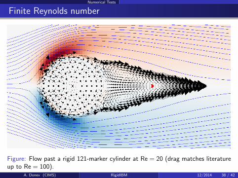
Finite Reynolds number
Figure: Flow past a rigid 121-marker cylinder at Re = 20 (drag matches literatureup to Re = 100).
A. Donev (CIMS) RigidIBM 12/2014 38 / 42
Outlook
Comparison to other methods
At the level of the formulation, for steady Stokes flow this is verysimilar to existing methods, e.g., Regularized Stokeslets.Main difference is that the mobility matrix in our formulation is SPD.
It also looks like a regularized first-kind boundary-elementformulation (so not very good!).Leslie Greengard and Manas Rachh are developing better second-kindmethods but thermal fluctuations require a bit more work.
The main difference with above is that we do not use Green’sfunctions but rely on a fluid solver; this works with various boundaryconditions, finite Reynolds numbers, variable viscosity flows.
Unlike Stokesian dynamics and related multipole-based methodssuch as Force Coupling Method this approach has controlledaccuracy (no ad hoc lubrication), but also more expensive.
The treatment of thermal fluctuations is similar to that in the popularLattice Boltzmann Method but the fluid solver here is verydifferent (allowing zero Reynolds and Mach numbers, for example).
A. Donev (CIMS) RigidIBM 12/2014 39 / 42

Outlook
FEM (Filtering)
We are presently working on using a Finite Element method torepresent the rigid body and the induced force density λ (q) usingstandard FEM basis functions.
In this approach by Boyce Griffith the IB markers are placed at theGauss nodes of the FEM mesh.
Algebraically this amounts to transforming the Schur complementfrom M to the filtered mobility
MFE = ΨMΨT ,
where Ψ is a sparse FEM assembly matrix that connects nodes of thegrid to Gauss points.
This filtering decreases the number of DOFs and improves theconditioning dramatically, and may lead to much improved strongconvergence (but still first order).
Effective preconditioning needs to be developed...
A. Donev (CIMS) RigidIBM 12/2014 40 / 42
Outlook
Future Directions
Develop fast solvers for RPY-like kernels (with Eric Darve)
Incorporate thermal fluctuations and develop stochastic integrationalgorithms (in progress).
Develop formulations more akin to (regularized) second-kind integralequations to get improved accuracy and conditioning.
Do active-body suspension applications (volunteers?).
A. Donev (CIMS) RigidIBM 12/2014 41 / 42
Outlook
References
Daisuke Takagi, Adam B Braunschweig, Jun Zhang, and Michael J Shelley.
Dispersion of self-propelled rods undergoing fluctuation-driven flips.Phys. Rev. Lett., 110(3):038301, 2013.
D. Bedeaux and P. Mazur.
Brownian motion and fluctuating hydrodynamics.Physica, 76(2):247–258, 1974.
Jose Garcıa de la Torre, Marıa L Huertas, and Beatriz Carrasco.
Calculation of hydrodynamic properties of globular proteins from their atomic-level structure.Biophysical Journal, 78(2):719–730, 2000.
F. Balboa Usabiaga, R. Delgado-Buscalioni, B. E. Griffith, and A. Donev.
Inertial Coupling Method for particles in an incompressible fluctuating fluid.Comput. Methods Appl. Mech. Engrg., 269:139–172, 2014.Code available at https://code.google.com/p/fluam.
M. Cai, A. J. Nonaka, J. B. Bell, B. E. Griffith, and A. Donev.
Efficient Variable-Coefficient Finite-Volume Stokes Solvers.16(5):1263–1297, 2014.Comm. in Comp. Phys. (CiCP).
B. Kallemov, A. Pal Singh Bhalla, B. E. Griffith, and A. Donev.
An immersed boundary method for suspensions of rigid bodies.In preparation, to be submitted to Comput. Methods Appl. Mech. Engrg., 2015.
A. Donev (CIMS) RigidIBM 12/2014 42 / 42


![A Fluctuating Boundary Integral Method for Brownian ...donev/FluctHydro/FBIM.pdf · possibility is to regularize the singularity, as done in the method of regularized Stokeslets [38]](https://cdn.vdocuments.net/doc/165x107/5f6439f8a6f41c720a53e1d3/a-fluctuating-boundary-integral-method-for-brownian-donevflucthydrofbimpdf.jpg)