
AN OPTIMIZATION STUDY ON CAVITY MAGNETRON
A THESIS SUBMITTED TO
THE GRADUATE SCHOOL OF NATURAL AND APPLIED SCIENCES
OF
MIDDLE EAST TECHNICAL UNIVERSITY
BY
MERVE KAYAN
IN PARTIAL FULFILLMENT OF THE REQUIREMENTS
FOR
THE DEGREE OF MASTER OF SCIENCE
IN
PHYSICS
JANUARY 2018

Approval of the thesis:
AN OPTIMIZATION STUDY ON CAVITY MAGNETRON
submitted by MERVE KAYAN in partial fulfillment of the requirements for the
degree of Master of Science in Physics Department, Middle East Technical
University by,
Prof. Dr. Gülbin Dural Ünver ________________
Dean, Graduate School of Natural and Applied Sciences
Prof. Dr. Altug Özpineci ________________
Head of Department, Physics
Assoc. Prof. Dr. Serhat Çakır ________________
Supervisor, Physics Department, METU
Examining Committee Members:
Prof. Dr. Enver Bulur ________________
Physics Department, METU
Assoc. Prof. Dr. Serhat Çakır ________________
Physics Department, METU
Assoc. Prof. Dr. İsmail Rafatov ________________
Physics Department, METU
Assoc. Prof. Dr. Alpan Bek ________________
Physics Department, METU
Assoc. Prof. Dr. Kemal Efe Eseller ________________
Electrical& Electronics Engineering Department,
Atilim University
Date: ________________

iv
I hereby declare that all information in this document has been obtained and
presented in accordance with academic rules and ethical conduct. I also
declare that, as required by these rules and conduct, I have fully cited and
referenced all material and results that are not original to this work.
Name, Last Name: MERVE KAYAN
Signature :

v
ABSTRACT
AN OPTIMIZATION STUDY ON CAVITY MAGNETRON
Kayan, Merve
M.S., Department of Physics
Supervisor: Assoc. Prof. Dr. Serhat Çakır
January 2018, 83 pages
We studied structure of cavity magnetrons and physics behind it deeply in this
thesis. The main purpose of this study is to observe parameters which affect
generated power of magnetron negatively or positively. Basically, they are crossed-
field devices and electrons generate RF power with the help of both electric and
magnetic field. We analyzed the physics of electron motion in magnetron and came
up with a power equation. Then, we studied a cylindrical hole-slot-type magnetron
with specific sizes and plotted curves to visualise which parameters have an effect
on power and how. It was determined as a result of analyzes that applied voltage
between the anode and cathode parts, resonator number, cathode radius and angular
resonant frequency are directly proportional with generated power. Contrary to
this, increase in gap factor and loaded quality factor decreases the generated power.
After all, for used magnetron and value range of parameters that we used, the
working values which give the maximum power generation are 0.5 for gap factor, 5
for the loaded quality factor and 2.2 cm for cathode radius. Moreover, much more

vi
number of resonator and higher angular resonant frequency provide much more
power generation.
Keywords: cavity magnetron, crossed-field devices, Helmholtz resonance
frequency

vii
ÖZ
OYUKLU MAGNETRON ÜZERİNDE OPTİMİZASYON ÇALIŞMASI
Kayan, Merve
Yüksek Lisans, Fizik Bölümü
Tez Yöneticisi: Doç. Dr. Serhat Çakır
Ocak 2018, 83 sayfa
Bu tezde, oyuklu magnetronların yapısını ve arkasındaki fiziği derinlemesine
inceledik. Bu çalışmanın asıl amacı magnetronun ürettiği gücü olumlu ya da
olumsuz etkileyen değişkenleri incelemek. Temel olarak magnetronlar çapraz
alanlı cihazlardır. Elektrik ve manyetik alanların yardımıyla elektronlar radyo
frekanslı güç üretirler. Magnetrondaki elektronların hareketini fiziksel olarak
çözümledik ve bir güç denklemine ulaştık. Sonra silindir biçiminde, belli ölçülere
sahip bir magnetron tasarladık ve hangi değişkenlerin çıkış gücünü etkilediğini ve
nasıl etkilediğini görselleştirmek için grafikler çizdik. Analizler sonucunda anot ve
katot kısımları arasında uygulanan voltajın, çınlayıcıların sayısının, katot
yarıçapının ve açısal rezonant frekansının çıkış gücüyle doğru orantılı olduğunu
belirlendi. Bunun aksine açıklık faktörü ve yüklü kalite faktöründeki artış çıkış
gücünü azalttı. Sonuç olarak kullandığımız magnetron ve parametrelerin değer
aralıkları için en yüksek güç üretimini sağlayan çalışma değerleri açıklık faktörü
için 0.5, yüklü kalite faktörü için 5 ve katot yarıçapı için 2.2 santimetredir. Ayrıca,

viii
daha fazla sayıda çınlayıcı ve daha yüksek açısal resonant frekansı daha fazla güç
üretimi sağlar.
Anahtar kelimeler: oyuklu magnetron, çapraz alanlı cihazlar, Helmholtz rezonans
frekansı

ix
To my family

x
ACKNOWLEDGMENTS
Above all, I owe my supervisor Assoc. Prof. Dr. Serhat Çakır a great debt of
gratitude for his guidance, incredible patience, criticism, endless support, advice
and continuous encouragement that enabled me to make this study. It would be
impossible to finish this thesis without him so I consider myself lucky to be able to
have worked under his mentorship.
I would also like to thank my unique family; my mother Belma Kayan, my father
Ömer Kayan and my brother Mustafa Barış Kayan for their endless support,
patience, compassionate and unconditional love. They were right beside me to
support like as they did always. To have them is the best side of me.
Additional thanks to all my colleagues and friends for their continuous support.
Especially, I am greatful to Mertcan Genç for his presence in my life for the last 8
years and for his endless love and support. He has always been there to make me
smile and happy.

xi
TABLE OF CONTENT
ABSTRACT ............................................................................................................... v
ÖZ ............................................................................................................................ vii
ACKNOWLEDGMENTS ........................................................................................ x
TABLE OF CONTENTS ......................................................................................... xi
LIST OF TABLES ................................................................................................. xiv
LIST OF FIGURES ................................................................................................ xv
CHAPTERS
1. INTRODUCTION ....................................................................................... 1
2. BASIC PHYSICS OF MAGNETRON ....................................................... 9
2.1 Impacts of Different Fields on Charged Particles .................................. 9
2.1.1 Motion in Electric Field .................................................................. 11
2.1.1.1 Cartesian Coordinate System .............................................. 11
2.1.1.2 Cylindrical Coordinate System ............................................ 17
2.1.2 Motion in Magnetic Field ............................................................... 21
2.1.2.1 Cartesian Coordinate System .............................................. 21
2.1.2.2 Cylindrical Coordinate System ............................................ 27

xii
2.1.3 Motion in both Magnetic and Electric Field ................................... 28
2.1.4 Motion in Magnetic, Electric and an AC Field ............................... 31
2.1.4.1 Cartesian Coordinate System ............................................... 32
2.1.4.2 Cylindrical Coordinate System ............................................ 38
2.2 Electron Motion in Magnetron ............................................................. 40
2.3 Hull Cutoff Equation for Magnetron ................................................... 42
2.4 Cyclotron Angular Frequency for an Electron ..................................... 42
2.5 Equivalent Circuit ................................................................................ 44
2.6 Quality Factor ...................................................................................... 45
2.7 Power and Efficiency ........................................................................... 46
3. PARAMETERS WHICH AFFECT THE GENERATED POWER .......... 49
3.1 Derivations of Some Important Parameters ......................................... 49
3.1.1 Electric Field ................................................................................... 50
3.1.2 The Capacitance at Vane Tips ........................................................ 50
3.1.3 Angular Resonant Frequency .......................................................... 51
3.1.4 Electrical Conductivity ................................................................... 55
3.2 Observations of Change in Power about Effects of Some Parameters 59
3.2.1 Effect of Cavity Number on Generated Power .............................. 61
3.2.2 Effect of Gap Factor on Generated Power ..................................... 63

xiii
3.2.3 Effect of Loaded Quality Factor on Generated Power .................. 66
3.2.4 Effect of Cathode Radius on Generated Power ............................. 69
3.2.5 Effect of Angular Resonant Frequency on Generated Power ........ 72
4. CONCLUSIONS & DISCUSSION .......................................................... 75
REFERENCES ....................................................................................................... 81

xiv
LIST OF TABLES
TABLES
Table 1 Conductivity values of different materials ................................................ 56
Table 2 Values of variables for cavity number-power graph ................................. 62
Table 3 Values of variables for gap factor-power graph ....................................... 63
Table 4 Values of variables for loaded quality factor-power graph ...................... 66
Table 5 Values of variables for cathode radius-power graph ................................ 69

xv
LIST OF FIGURES
FIGURES
Figure 1 Hull’s magnetron model ............................................................................ 2
Figure 2 Habann’s split-anode magnetron ............................................................... 2
Figure 3 Multi-cavity magnetron of Hollmann ....................................................... 3
Figure 4 Randall and Boot’s multi-cavity magnetron ............................................ 3
Figure 5 Basic construction of magnetron ............................................................... 4
Figure 6 One of the resonant cavities ...................................................................... 4
Figure 7 Common cavity types ................................................................................ 5
Figure 8 Strapping alternate segments ..................................................................... 6
Figure 9 Influence of magnetic field on path of electron ........................................ 6
Figure 10 Microwave oven structure ....................................................................... 7
Figure 11 Radar system .......................................................................................... 8
Figure 12 (a) E field between the parallel plates (b) direction of electron ........... 12
Figure 13 (a) Geometry of cylindrical diode and potentials (b) crosscut and
electric field .......................................................................................... 17
Figure 14 Straight motion of electron in magnetron .............................................. 21
Figure 15 (a) B field between the parallel plates (b) direction of electrons with
different velocities ................................................................................ 21
Figure 16 (a) Geometry of cylindrical diode and field (b) direction of electrons
with different velocities ......................................................................... 28

xvi
Figure 17 Electron motion in both magnetic and electric fields ............................ 30
Figure 18 (a) View of cavity in the magnetron (b) equivalent parallel resonant
circuit of magnetron cavity ................................................................... 31
Figure 19 E, B and an AC field between the parallel plates .................................. 32
Figure 20 Movement of the point on the circumference of the wheel ................... 36
Figure 21 Charged particle motion in the combined field .................................... 38
Figure 22 Electron paths in magnetron ................................................................. 39
Figure 23 Force lines of an 8-cavity magnetron in π-mode .................................. 43
Figure 24 Equivalent circuit for magnetrons resonator ......................................... 44
Figure 25 Capacitor and parallel plates with E field .............................................. 50
Figure 26 Cavity resonant ...................................................................................... 51
Figure 27 View of simple example of cavity resonator ......................................... 52
Figure 28 Equivalent spring-mass system ............................................................. 52
Figure 29 Simple circuit ......................................................................................... 57
Figure 30 View of resistor ..................................................................................... 57
Figure 31 Used 8 cavity magnetron for our work ................................................. 60
Figure 32 Cavity Number versus Generated Power Graph .................................... 62
Figure 33 Gap Factor versus Generated Power Graph .......................................... 64
Figure 34 Gap Factor versus 1st Derivative of Power Graph ................................. 65
Figure 35 Gap Factor versus 2nd Derivative of Power Graph ................................ 65
Figure 36 Loaded Quality Factor versus Generated Power Graph ........................ 67
Figure 37 Loaded Quality Factor versus 1st Derivative of Power Graph............... 68
Figure 38 Loaded Quality Factor versus 2nd Derivative of Power Graph .............. 68
xvii
Figure 39 Cathode Radius versus Generated Power Graph ................................... 70
Figure 40 Cathode Radius versus 1st Derivative of Power Graph ......................... 71
Figure 41 Cathode Radius versus 2nd Derivative of Power Graph ........................ 71
Figure 42 Angular Resonant Frequency versus Generated Power Graph ............. 73
Figure 43 Electron motion in magnetron ............................................................... 76

xviii

1
CHAPTER 1
INTRODUCTION
There are two groups of microwave devices. First one is semiconductor devices
which are Gunn diode, backward diode, tunnel diode, IMPATT (impact ionization
avalanche transit time operation) diode, Schottky diode, varactor diode, PIN diode
(p-i-n diode), transistors and integrated circuits (ICs). Second one is tube devices
which are klystron, reflex klystron, traveling wave tube (TWT) and magnetron. It
is more cheaply to generate and amplify high levels of microwave signals with tube
devices. In this thesis, the aim is to analyze the cavity magnetron deeply.
During the last century, different types of microwave vacuum equipment have been
used as an amplifier or a generator in many different areas such as: medical X-ray
sources, microwave heating, communication, warfare and radar [1]. Magnetron is
the most promising and popular high power microwave device because of some
advantages of it. For example, it has a small size, light weight and low-cost [2].
Another positive aspect of magnetron is that it can generate high power in the range
of kilowatts to megawatts. Moreover, it works with a high efficiency around 40 to
70% [3]. Magnetron is a self-excitation vacuum tube oscillator. It uses electrons
with the magnetic fields and converts energy of electrons to high power
radiofrequency signals [4].
The developments about the magnetron began with Heinrich Greinacher, a Swiss
physicist, in 1912. He gave some basic mathematical definition about the motion of
electrons in a magnetic field. In 1921, Albert Wallace Hull observed that the motion
of electrons to the anode can be controlled with the influence of magnetic field.

2
Figure 1: Hull’s magnetron model [5]
Actually, he was in a competition with the opponent company and wanted to invent
an amplifier that is controlled magnetically. However, he noticed the chance of
radiofrequency generation and called his invention as magnetron (Fig. 1). Then in
1924, Erich Habann from Germany and Napsal August Zázek from Czechia have
studied on magnetron independently. Habann used steady magnetic field as today’s
magnetrons and observed oscillations in the range of 100 MHz with his split-anode
magnetron (Fig. 2).
Figure 2: Habann’s split-anode magnetron [5]
Zázek has developed a magnetron that operated in the range of 1 GHz. Kinjiro
Okabe from Tohoku University took a big step by developing a magnetron with the
range of 5.35 GHz in 1929. Hans Erich Hollmann improved a multi-cavity
magnetron and in 1938 he was granted a patent on multi-cavity magnetron in
Germany (Fig. 3).

3
Figure 3: Multi-cavity magnetron of Hollmann [5]
In 1940s, engineer John Randall and Henry Boot built a multi-cavity magnetron
and with this invention, England gained an advantage over Germany in the sub-
marine war. These two engineers made a magnetron with more than four cavities to
increase the efficiency of the radiofrequency generation (Fig. 4). In the meantime,
Henry Gutton was studying about the cathodes made with barium oxide in multi-
cavity magnetrons and he observed that barium oxide cathode needs lower
temperature to release electron when it compared with the tungsten cathodes. In
other words, this observed characteristic prolongs the magnetron life. John Randall
and Henry Boot used this result in their own investigations [5].
Figure 4: Randall and Boot’s multi-cavity magnetron [5]
Physical structure of magnetron can be separated into three main parts: anode,
cathode and filament and interaction space. Fig. 5 shows these parts with cavities
and an output lead.

4
Figure 5: Basic construction of magnetron [6]
The anode part of magnetron is made from solid copper. As shown, it is a cylindrical
block and surrounds the cathode. Each seen hole is called as a resonant cavity and
they work like a parallel resonant circuit which shown in Fig. 6. The rear wall of
cavity is thought as an inductive portion, like a coil with single turn and the vane
tip is thought as a capacitor. The physical dimensions of the resonator determine
the resonant frequency.
Figure 6: One of the resonant cavities [6]

5
A single oscillated resonant cavity excites the next cavity and it oscillates too.
Effected one oscillates with a phase delay, which is 180 degrees. Then, these
interactions continue similarly. This continued actions form a closed slow-wave
structure. Because of this feature, sometimes we use the name of “Multi-cavity
Travelling Wave Magnetron” for this design. Cathode and filament are placed at
the center of the magnetron and filament leads fix them in their positions with the
help of leads’ rigid and large structure. Cathode has a shape like a hollow cylinder
and high emission material is used for it (like barium oxide). Cathode part of
magnetron provides electron that is required for energy transfer. At the center of
the cathode, there is a feeding wire of the filament. If an eccentricity occurs between
the cathode and anode, malfunction or an internal arcing takes place, which is an
undesired event. Interaction space is the entire area between the cathode and the
anode block. In this space, magnetic and electric fields affect each other and this
causes a force on electrons. Around the magnetron, a magnet is mounted and this
creates a magnetic field, which is parallel with the cathode axis [6].
Figure 7: Common cavity types [7]
Three common types of cavity forms are illustrated in Fig. 7. Here, A is the hole-
slot-type, B is the vane-type, C is the rising-sun-type. For hole-slot and vane types,
cavities are connected each other with straps as shown. However, there is not any
straps in the rising sun type. About hole-slot and vane types, there should be
connected alternate segments, in order that side-by-side segments have opposite
poles. Therefore, they have even number of cavities. This shown in Fig. 8. For
A B C

6
rising-sun-type, large and small trapezoidal cavities are aligned respectively and
this provides a stable frequency between the resonant frequencies of all cavities [7].
Figure 8: Strapping alternate segments [7]
About magnetrons, we can say that they are crossed-field devices. Electrons are
released from cathode and the electric field accelerates them. After electrons
increase their velocity so they gain energy, electrons direction is oblique by the
magnetic field, which is perpendicular to electric field [3]. The reason of the
magnetic field is the magnet placed around the magnetron. Cathode of magnetron
has a negative voltage so electric field moves from the anode block to the cathode
in radial direction. If there is not any magnetic field and cathode is heated, electrons
move to the anode directly and uniformly as shown in Fig. 9 with the blue path.
Figure 9: Influence of magnetic field on path of electron [6]

7
Electrons bends like the green path in Fig. 9 when magnetic field is weak and
permanent. To have flowing plate current, electrons should reach the anode block.
If we enhance the magnetic field, electrons bend sharply. Similarly, increasing the
electron velocity causes an increase on the field around it and path of electrons have
sharper bend. As shown in the Fig. 9 as a red path, when magnetic field reaches the
critical value, electrons return to cathode without reaching the anode block. At that
case, plate current drop off to a very small value. If applied magnetic field is bigger
than the critical value, plate current reaches to zero. If electrons cannot reach the
anode, oscillations at microwave frequencies can be produced. In other words,
magnetrons work like a magnetic mirror and they trap high temperature plasma with
the helping of magnetic field.
It is mentioned that magnetrons are used in countless applications. Fig. 10 shows
the one of these, microwave oven. Microwave oven systems can be seperated in
three parts. These are microwave source which is magnetron, waveguide feed and
an oven space. Operation of microwave oven stars with the microwave generator,
magnetron. Electricity comes from power outlet to the magnetron.
Figure 10: Microwave oven structure
8
Then, it transforms this energy to the high powered radio waves [8]. This magnetron
works at 2.45 GHz and it produces an output power in the range of 500-1500 W.
These waves reaches to the oven space with a waveguide feed and microwave cooks
the foods on the rotating plate [3]. The working principle of magnetron will explain
in the next chapters.
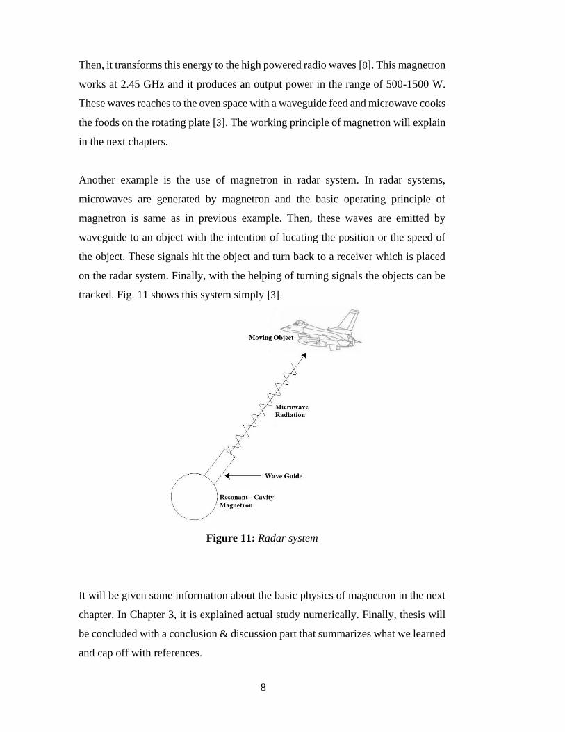
Another example is the use of magnetron in radar system. In radar systems,
microwaves are generated by magnetron and the basic operating principle of
magnetron is same as in previous example. Then, these waves are emitted by
waveguide to an object with the intention of locating the position or the speed of
the object. These signals hit the object and turn back to a receiver which is placed
on the radar system. Finally, with the helping of turning signals the objects can be
tracked. Fig. 11 shows this system simply [3].
Figure 11: Radar system
It will be given some information about the basic physics of magnetron in the next
chapter. In Chapter 3, it is explained actual study numerically. Finally, thesis will
be concluded with a conclusion & discussion part that summarizes what we learned
and cap off with references.
9
CHAPTER 2
BASIC PHYSICS OF MAGNETRON
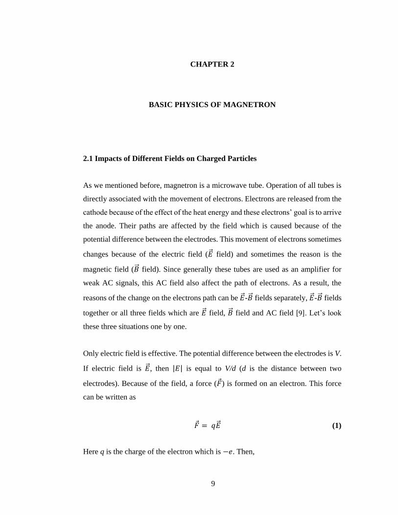
2.1 Impacts of Different Fields on Charged Particles
As we mentioned before, magnetron is a microwave tube. Operation of all tubes is
directly associated with the movement of electrons. Electrons are released from the
cathode because of the effect of the heat energy and these electrons’ goal is to arrive
the anode. Their paths are affected by the field which is caused because of the
potential difference between the electrodes. This movement of electrons sometimes
changes because of the electric field (�⃗� field) and sometimes the reason is the
magnetic field (�⃗� field). Since generally these tubes are used as an amplifier for
weak AC signals, this AC field also affect the path of electrons. As a result, the
reasons of the change on the electrons path can be �⃗� -�⃗� fields separately, �⃗� -�⃗� fields
together or all three fields which are �⃗� field, �⃗� field and AC field [9]. Let’s look
these three situations one by one.
Only electric field is effective. The potential difference between the electrodes is V.
If electric field is �⃗� , then |𝐸| is equal to V/d (d is the distance between two
electrodes). Because of the field, a force (𝐹 ) is formed on an electron. This force
can be written as
𝐹 = 𝑞�⃗� (1)
Here q is the charge of the electron which is −𝑒. Then,

10
𝐹 = −𝑒�⃗� (2)
As seen in Eq. 2, it is not important whether electron is moving or not.
If there is only magnetic field and electrons velocity is 𝑣 , then the force on an
electron become
𝐹 = −𝑒(𝑣 × �⃗� ) (3)
This means, we can talk about the magnetic field effect if the particle is moving.
So 𝑣 ≠ 0 is the case for the �⃗� field effect. Here the force is perpendicular not only
to electron velocity, but also to �⃗� field.
If there are both electric and magnetic fields, the force on an electron can be
obtained by summing Eq.2 and Eq.3. So
𝐹 = −𝑒[�⃗� + (𝑣 × �⃗� )] (4)
The Eq.4 is also called as Lorentz Force equation.
Like it is mentioned before, sometimes these tubes is used as an amplifier. In this
case, we have to consider the AC field which is 𝐸′ cos(𝑤𝑡). Let’s assume this field
direction is same with the �⃗� field direction. Then, Eq.4 becomes
𝐹 = −𝑒[(�⃗� + �⃗� ′ cos𝑤𝑡) + (𝑣 × �⃗� )] (5)
Here 𝐸′ is the value for AC field and 𝑤 is used for the angular frequency. So force
in Eq.5 is caused by E field, B field and AC field.

11
This force equation can change because of the tube shape. Moreover, E or B field
can be one dimensional or two or three. This also affects the force equation.
However, about these fields, it is assumed that they have only one component.
Besides, tube shapes cause to use the Cartesian or cylindrical systems generally [9].
2.1.1 Motion in Electric Field
If there is an electric field, the force value is also equal to the change of momentum
in time. Then Eq.2 can be written as
𝐹 = −𝑒�⃗� =𝑑
𝑑𝑡(𝑚𝑣 ) = 𝑚
𝑑�⃗�
𝑑𝑡 (6)
Here, 𝑣 is the velocity and m is the mass of the particle. Eq.6 is the general equality
and this form can be used for any system.
2.1.1.1 Cartesian Coordinate System
In this case, both E and B field has three components. Then Eq.6 can be rewritten
as
−𝑒𝐸𝑥 = 𝑚𝑑𝑣𝑥
𝑑𝑡= 𝑚
𝑑2𝑥
𝑑𝑡2 (7)
−𝑒𝐸𝑦 = 𝑚𝑑𝑣𝑦
𝑑𝑡= 𝑚
𝑑2𝑦
𝑑𝑡2 (8)
−𝑒𝐸𝑧 = 𝑚𝑑𝑣𝑧
𝑑𝑡= 𝑚
𝑑2𝑧
𝑑𝑡2 (9)
Here x, y and z are components of position vector and 𝑣𝑥, 𝑣𝑦 ve 𝑣𝑧 are components
of the velocity vector.
In Fig. 12a plates are located at 𝑥 = 0 and 𝑥 = 𝑑. Potentials are equal to zero for
bottom plate and 𝑉0 for upper plate. Let’s assume that when electron enters the E

12
field at time t=0, its position is at x=y=z=0 and its initial velocities are 𝑣𝑥 = 𝑣𝑥0,
𝑣𝑦 = 𝑣𝑦0 and 𝑣𝑧 = 0. For E field, 𝐸𝑥 equals to −𝑉0 𝑑⁄ and the other components
are equal to zero.
Figure 12: (a) E field between the parallel plates (b) direction of electron
By using the Eq.7, Eq.8 and Eq.9 we can write
𝑑𝑣𝑥
𝑑𝑡=
𝑑2𝑥
𝑑𝑡2 = −𝑒
𝑚𝐸𝑥 = −
𝑒
𝑚(−
𝑉0
𝑑) =
𝑒𝑉0
𝑚𝑑= 𝑘 (10)
𝑑𝑣𝑦
𝑑𝑡=
𝑑2𝑦
𝑑𝑡2 = 0 (11)
𝑑𝑣𝑧
𝑑𝑡=
𝑑2𝑧
𝑑𝑡2 = 0 (12)
Let’s solve these last three equations:
From equations 10, 11 and 12, we can write
𝑥 =1
2𝑘𝑡2 + 𝐴1𝑡 + 𝐵1 (13a)
𝑦 = 𝐴2𝑡 + 𝐵2 (13b)

13
𝑧 = 𝐴3𝑡 + 𝐵3 (13c)
Initially, we know that at 𝑡 = 0, 𝑥 = 𝑦 = 𝑧 = 0. Then this means that 𝐵1 = 𝐵2 =
𝐵3 = 0 and Eq.13 becomes
𝑥 =1
2𝑘𝑡2 + 𝐴1𝑡 (14a)
𝑦 = 𝐴2𝑡 (14b)
𝑧 = 𝐴3𝑡 (14c)
If we take the derivatives of x, y and z, we obtain
𝑑𝑥
𝑑𝑡= 𝑘𝑡 + 𝐴1 (15a)
𝑑𝑦
𝑑𝑡= 𝐴2 (15b)
𝑑𝑧
𝑑𝑡= 𝐴3 (15c)
Another condition is that at 𝑡 = 0, 𝑣𝑥 = 𝑣𝑥0, 𝑣𝑦 = 𝑣𝑦0
and 𝑣𝑧 = 0 so
𝐴1 = 𝑣𝑥0 (16a)
𝐴2 = 𝑣𝑦0 (16b)
𝐴3 = 0 (16c)
Then Eq.14 reduces to
𝑥 =1
2𝑘𝑡2 + 𝑣𝑥0
𝑡 (17a)

14
𝑦 = 𝑣𝑦0𝑡 (17b)
𝑧 = 0 (17c)
We know that 𝑘 = 𝑒𝑉0 𝑚𝑑⁄ , then Eq.17 can be written as
𝑥 = (𝑒𝑉0
2𝑚𝑑) 𝑡2 + 𝑣𝑥0
𝑡 and 𝑣𝑥0𝑡 = 𝑥 − (
𝑒𝑉0
2𝑚𝑑) 𝑡2 (18a)
𝑦 = 𝑣𝑦0𝑡 and 𝑡 =
𝑦
𝑣𝑦0
(18b)
If we use the ‘𝑡’ value in Eq.18b, Eq.18a becomes
𝑥 = (𝑒𝑉0
2𝑚𝑑) (
𝑦
𝑣𝑦0
)2
+ 𝑣𝑥0(
𝑦
𝑣𝑦0
) (19)
Here Eq.19 is a parabola equation in the x-y plane and we know that
𝑣𝑥 =𝑑𝑥
𝑑𝑡= (
𝑒𝑉0
𝑚𝑑) 𝑡 + 𝑣𝑥0
(20a)
𝑣𝑦 =𝑑𝑦
𝑑𝑡= 𝑣𝑦0
(20b)
𝑣𝑧 =𝑑𝑧
𝑑𝑡= 0 (20c)
Then
𝑣 = √(𝑣𝑥2 + 𝑣𝑦
2) = √𝑣𝑦02 + [(
𝑒𝑉0
𝑚𝑑) 𝑡 + 𝑣𝑥0
]2 (21a)
𝑣 = √𝑣𝑦02 + [(
𝑒𝑉0
𝑚𝑑)2𝑡2 + 2(
𝑒𝑉0
𝑚𝑑) 𝑣𝑥0
𝑡 + 𝑣𝑥02 ] (21b)

15
If we use 𝑣𝑥0𝑡 = 𝑥 − (𝑒𝑉0/2𝑚𝑑)𝑡2 in Eq.21, we get
𝑣 = √𝑣𝑦02 + (
𝑒𝑉0
𝑚𝑑)2𝑡2 + (
2𝑒𝑉0
𝑚𝑑) 𝑥 − (
𝑒𝑉0
𝑚𝑑)2𝑡2 + 𝑣𝑥0
2 (22a)
𝑣 = √𝑣𝑥02 + 𝑣𝑦0
2 + (2𝑒𝑉0
𝑚𝑑) 𝑥 (22b)
The kinetic energy at 𝑡 = 0 is 𝐾𝐸0. When 𝑡 equals to zero and 𝑥 = 0 if we use
Eq.22b then the kinetic energy becomes
𝐾𝐸0 =1
2𝑚𝑣2 =
1
2𝑚(𝑣𝑥0
2 + 𝑣𝑦02 ) (23)
At any time ‘𝑡’, the kinetic energy is written as
𝐾𝐸𝑡 =1
2𝑚 [𝑣𝑥0
2 + 𝑣𝑦02 + (
2𝑒𝑉0
𝑚𝑑) 𝑥] (24)
The difference between Eq.23 and Eq.24 gives the gained energy in time ‘𝑡’ and
this is
∆𝐾𝐸 =1
2𝑚(
2𝑒𝑉0
𝑚𝑑) 𝑥 = (
𝑒𝑉0
𝑑) 𝑥 (25)
The potential energy of electron with an ‘𝑥’ displacement is that
−𝑒𝑉 = −𝑒 (𝑉0
𝑑) 𝑥 = −∆𝐾𝐸 (26)
The minus sign in Eq.26 means that any decrease in potential energy is compensated
by the increase in 𝐾𝐸.

16
If initially velocities are taken as zero, this means that 𝑣𝑥𝑜= 𝑣𝑦𝑜
= 0, then
𝑣 = √2𝑒𝑉 𝑚⁄ (27)
where 𝑉 = 𝐸. 𝑥 = 𝑉0. 𝑥 𝑑⁄ and here x is again the position component in the x-
direction.
Eq.27 is the solution of Eq.10, Eq.11, Eq.12 and if we substitute the constant values
(𝑒 = 1.602 × 10⁻¹⁹ C and 𝑚 = 9.1091 × 10⁻³¹ kg) into the Eq.27, we obtain
𝑣 = 5.932 × 10⁵√𝑉0𝑥
𝑑 𝑚/𝑠 (28)
For example, we can find the velocity at 𝑥 = 𝑑 as
𝑣 = 0.5932 × 10⁶√𝑉0 𝑚/𝑠 (29)
It is mentioned that 𝐹 = 𝑞�⃗� so electric field is proportional to force directly.
Therefore, electrons move from the cathode to the anode directly. Fig. 12b shows
the movement of electron in E field between two plates.

17
2.1.1.2 Cylindrical Coordinate System
Figure 13: (a) Geometry of cylindrical diode and potentials (b) crosscut and E
field
Fig. 13 shows the diode geometry in a cylindrical system. Moreover, it also shows
the E field lines and moving direction of electron. In this case, 𝑣 is three
dimensional and 𝑣 = 𝑣𝑟𝑎�̂� + 𝑣∅𝑎∅̂ + 𝑣𝑧𝑎�̂�.Then, Eq.6 can be rewritten as
−𝑒
𝑚�⃗� =
𝑑
𝑑𝑡(𝑣𝑟𝑎�̂� + 𝑣∅𝑎∅̂ + 𝑣𝑍𝑎�̂�) =
𝑑
𝑑𝑡(𝑣𝑟𝑎�̂�) +
𝑑
𝑑𝑡(𝑣∅𝑎∅̂) +
𝑑
𝑑𝑡(𝑣𝑧𝑎�̂�) (30)
Here 𝑣𝑟,∅,𝑧 are velocities and 𝑣𝑟 = 𝑑𝑟 𝑑𝑡⁄ , 𝑣∅ = 𝑟𝑑∅ 𝑑𝑡⁄ and 𝑣𝑍 = 𝑑𝑧 𝑑𝑡⁄ .
Moreover, 𝑎𝑟,∅,𝑧 are the unit vectors.
Three terms in Eq.30 become
𝑑
𝑑𝑡(𝑣𝑟𝑎�̂�) = 𝑣𝑟
𝑑∅
𝑑𝑡𝑎∅̂ +
𝑑𝑣𝑟
𝑑𝑡𝑎�̂� (31)
𝑑
𝑑𝑡(𝑣∅𝑎∅̂) = −𝑣∅
𝑑∅
𝑑𝑡𝑎�̂� +
𝑑𝑣∅
𝑑𝑡𝑎∅̂ (32)
𝑑
𝑑𝑡(𝑣𝑧𝑎�̂�) =
𝑑𝑣𝑧
𝑑𝑡𝑎�̂� (33)

18
By using Eq.30, Eq.31, Eq.32 and Eq.33, we can write
−𝑒
𝑚𝐸𝑟 =
𝑑𝑣𝑟
𝑑𝑡− 𝑣∅
𝑑∅
𝑑𝑡 (34)
−𝑒
𝑚𝐸∅ = 𝑣𝑟
𝑑∅
𝑑𝑡+
𝑑𝑣∅
𝑑𝑡 (35)
−𝑒
𝑚𝐸𝑧 =
𝑑𝑣𝑧
𝑑𝑡 (36)
Let’s find a solution for equations 34, 35 and 36:
𝑣 can be written as
𝑣 = 𝑣𝑟𝑎�̂� + 𝑣∅𝑎∅̂ + 𝑣𝑧𝑎�̂� =𝑑𝑟
𝑑𝑡𝑎�̂� +
𝑟𝑑∅
𝑑𝑡𝑎∅̂ +
𝑑𝑧
𝑑𝑡𝑎�̂� (37)
Here 𝑑∅ 𝑑𝑡 = 𝑤⁄ and 𝑣∅ = 𝑟𝑤, then equations 34, 35 and 36 transform to
−𝑒
𝑚𝐸𝑟 =
𝑑2𝑟
𝑑𝑡2 − 𝑟𝑤2 (38a)
−𝑒
𝑚𝐸∅ = 𝑤
𝑑𝑟
𝑑𝑡+
𝑑(𝑤𝑟)
𝑑𝑡=
1
𝑟
𝑑
𝑑𝑡(𝑟2𝑤) (38b)
−𝑒
𝑚𝐸𝑧 =
𝑑2𝑧
𝑑𝑡2 (38c)
We mentioned that for this case, the motion of particle in E-field can be seen in
Fig. 13 which also shows the radiuses and voltages of both cylinders. Then, the
potential relation can be given as
𝑉 = 𝑉0ln 𝑟/𝑎
ln𝑏/𝑎 (39)
here 𝑎 is cathode radius, 𝑏 is anode radius and

19
𝐸𝑟 = −𝜕𝑉
𝜕𝑟= −𝑉0
1
𝑟 ln𝑏/𝑎 (40a)
𝐸∅ = 𝐸𝑧 = 0 (40b)
If we consider Eq.40, Eq.38 becomes
−𝑒𝑉0
𝑚𝑟 ln𝑏/𝑎=
𝑘
𝑟=
𝑑2𝑟
𝑑𝑡2 − 𝑟𝑤2 (41a)
𝑑(𝑟2𝑤)
𝑑𝑡= 0 (41b)
𝑑2𝑧
𝑑𝑡2 = 0 (41c)
Let’s assume, an electron which initially has a velocity 𝑣 = 0 enters the E-field at
𝑡 = 0 and its position is 𝑟 = 𝑎, ∅ = 0 and 𝑧 = 0. From Eq.38c, 𝑧 is zero for all ‘𝑡’
values. Besides, for Eq.38b assume that 𝑟2𝑤 = 𝑟 × 𝑟𝑤 = 𝑟 × 𝑣∅ = 𝐴. We know
that 𝑣 = 0 when 𝑡 equals to zero, then 𝐴 = 0 or 𝑤 = 0 for all ‘𝑡’ values.
Also 𝑣𝑟 = 𝑑𝑟 𝑑𝑡⁄ means that 𝑑𝑡 equals to 𝑑𝑟 𝑣𝑟⁄ . Then, Eq.38a can be written as
𝑑2𝑟
𝑑𝑡2 =𝑑𝑣𝑟
𝑑𝑡=
𝑘
𝑟 (42a)
𝑑𝑣𝑟 = (𝑘
𝑟) 𝑑𝑡 = (
𝑘
𝑟) (
𝑑𝑟
𝑣𝑟) or 𝑣𝑟𝑑𝑣𝑟 = (
𝑘
𝑟) 𝑑𝑟 (42b)
If we integrate both sides of Eq.42b we get
1
2𝑣𝑟
2 = 𝑘 ln 𝑟 + 𝐵 (43)
When we use the condition 𝑣𝑟 equals to zero at 𝑟 = 𝑎, value of 𝐵 becomes −𝑘 ln 𝑎.
Therefore,

20
1
2𝑣𝑟
2 =kln (𝑟
𝑎) (44a)
So
𝑣𝑟 = √[2𝑘 ln (𝑟
𝑎)] (44b)
If we substitute 𝑘 value into Eq.44b, finally we get
𝑣𝑟 =𝑑𝑟
𝑑𝑡= √
2𝑒𝑉0 ln(𝑟
𝑎)
𝑚 ln(𝑏
𝑎)
(45)
When we solve the equations 34, 35 and 36, we get Eq.45. Also we mentioned
that 𝑒 = 1.602 × 10⁻¹⁹ C and 𝑚 = 9.1091 × 10⁻³¹ kg. Then Eq.45 becomes
𝑣𝑟 = [5.932 × 10⁵√ln(𝑟 𝑎⁄ )
ln(𝑏 𝑎⁄ )]√𝑉0 𝑚/𝑠 (46)
If electron is at the cathode surface so if 𝑟 = 𝑎, the velocity value (𝑣) becomes zero.
However, when electron reaches to the anode surface, Eq.46 becomes
𝑣𝑟 = 5.932 × 10⁵√𝑉0 𝑚/𝑠 (47)
The values of velocity in Eq.29 and Eq.47 are same for a given voltage. Likely in
the Cartesian case, the electron path from the cathode is direct to the anode in
cylindrical system. For a magnetron, a view of impact of E field on an electron
motion is shown in Fig. 14 [9].
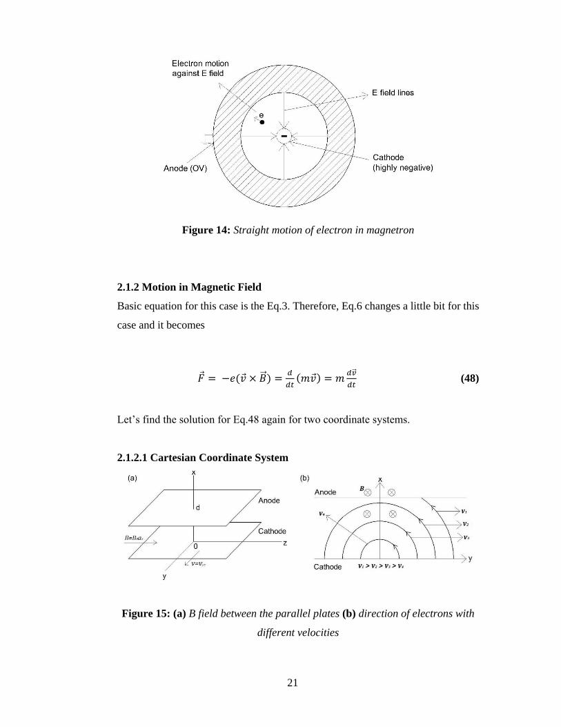
21
Figure 14: Straight motion of electron in magnetron
2.1.2 Motion in Magnetic Field
Basic equation for this case is the Eq.3. Therefore, Eq.6 changes a little bit for this
case and it becomes
𝐹 = −𝑒(𝑣 × �⃗� ) =𝑑
𝑑𝑡(𝑚𝑣 ) = 𝑚
𝑑�⃗�
𝑑𝑡 (48)
Let’s find the solution for Eq.48 again for two coordinate systems.
2.1.2.1 Cartesian Coordinate System
Figure 15: (a) B field between the parallel plates (b) direction of electrons with
different velocities

22
The structure of this case is shown in Fig. 15a. Here velocity is again there
component and it can be written like 𝑣 = 𝑣𝑥𝑎�̂� + 𝑣𝑦𝑎�̂� + 𝑣𝑧𝑎�̂�. Likewise, the
magnetic field vector is �⃗� = 𝐵𝑥𝑎�̂� + 𝐵𝑦𝑎�̂� + 𝐵𝑧𝑎�̂�.
When we use 𝑣 and �⃗� in Eq.48 with all these three components, we obtain
𝑑𝑣𝑥
𝑑𝑡=
−𝑒
𝑚(𝑣𝑦𝐵𝑧 − 𝑣𝑧𝐵𝑦) (49)
𝑑𝑣𝑦
𝑑𝑡=
−𝑒
𝑚(𝑣𝑧𝐵𝑥 − 𝑣𝑥𝐵𝑧) (50)
𝑑𝑣𝑧
𝑑𝑡=
−𝑒
𝑚(𝑣𝑥𝐵𝑦 − 𝑣𝑦𝐵𝑥) (51)
Because the first derivative of the position vector is the velocity vector, we can
change the form of Eq.49, Eq.50 and Eq.51 and they become
𝑑2𝑥
𝑑𝑡2 =−𝑒
𝑚(𝐵𝑧
𝑑𝑦
𝑑𝑡− 𝐵𝑦
𝑑𝑧
𝑑𝑡) (52)
𝑑2𝑦
𝑑𝑡2 =−𝑒
𝑚(𝐵𝑥
𝑑𝑧
𝑑𝑡− 𝐵𝑧
𝑑𝑥
𝑑𝑡) (53)
𝑑2𝑧
𝑑𝑡2 =−𝑒
𝑚(𝐵𝑦
𝑑𝑥
𝑑𝑡− 𝐵𝑥
𝑑𝑦
𝑑𝑡) (54)
Let’s find the solution of equations from 49 to 54:
Assume that �⃗� = 𝐵0𝑎𝑧 ̂and an electron that has the velocity 𝑣 = 𝑣𝑦0𝑎�̂� initially
enters the magnetic field at the position of 𝑥 = 𝑦 = 𝑧 = 0. Also 𝑧 is zero for all
times because 𝑧 component of 𝑣 is zero and 𝑥 component of 𝑣 is zero at 𝑡 = 0. Then
Eq.52, Eq.53 and Eq.54 transform to
𝑑2𝑥
𝑑𝑡2 = −𝑒
𝑚𝐵0
𝑑𝑦
𝑑𝑡 (55a)

23
so
𝑑𝑦
𝑑𝑡= −
𝑚
𝑒𝐵0
𝑑2𝑥
𝑑𝑡2 (55b)
𝑑2𝑦
𝑑𝑡2 =𝑒
𝑚𝐵0
𝑑𝑥
𝑑𝑡 (55c)
so
𝑑𝑥
𝑑𝑡=
𝑚
𝑒𝐵0
𝑑2𝑦
𝑑𝑡2 (55d)
and
𝑑2𝑧
𝑑𝑡2 = 0 (55e)
If we use 𝑑𝑦 𝑑𝑡⁄ value in Eq.55c and 𝑑𝑥 𝑑𝑡⁄ value in Eq.55a, we get
𝑑2𝑦
𝑑𝑡2 = −𝑚
𝑒𝐵0
𝑑3𝑥
𝑑𝑡3 =𝑒𝐵0
𝑚
𝑑𝑥
𝑑𝑡 (56a)
𝑑2𝑥
𝑑𝑡2 =𝑚
𝑒𝐵0
𝑑3𝑦
𝑑𝑡3 = −𝑒𝐵0
𝑚
𝑑𝑦
𝑑𝑡 (56b)
We can change the form of Eq.56 and it turns to
𝑑2𝑣𝑥
𝑑𝑡2 = −(𝑒𝐵0
𝑚)2𝑣𝑥 and
𝑑2𝑣𝑥
𝑑𝑡2 + 𝑤02𝑣𝑥 = 0 (57a)
𝑑2𝑣𝑦
𝑑𝑡2 = −(𝑒𝐵0
𝑚)2𝑣𝑦 and
𝑑2𝑣𝑦
𝑑𝑡2 + 𝑤02𝑣𝑦 = 0 (57b)
where 𝑤0 = 𝑒𝐵0/𝑚.
The solution of Eq.57 is
𝑣𝑥 = 𝐴1 cos𝑤0𝑡 + 𝐵1 sin𝑤0𝑡 (58a)

24
𝑣𝑦 = 𝐴2 cos𝑤0𝑡 + 𝐵2 sin𝑤0𝑡 (58b)
Use conditions;
When 𝑡 = 0, 𝑣𝑥 is also zero then 𝐴1 = 0. So Eq.58a turns to
𝑣𝑥 = 𝐵1 sin𝑤0𝑡 (59a)
When 𝑡 = 0, 𝑣𝑦 equals to 𝑣𝑦0 then 𝐴2 = 𝑣𝑦0
. So Eq.58b turns to
𝑣𝑦 = 𝑣𝑦0cos𝑤0𝑡 + 𝐵2 sin𝑤0𝑡 (59b)
With all these, Eq.55a and Eq.55c can be written as
𝑑2𝑥
𝑑𝑡2 = −𝑒
𝑚𝐵0
𝑑𝑦
𝑑𝑡 so
𝑑𝑣𝑥
𝑑𝑡= −
𝑒
𝑚𝐵0𝑣𝑦 = −𝑤0𝑣𝑦 (60a)
and
𝑑2𝑦
𝑑𝑡2 =𝑒
𝑚𝐵0
𝑑𝑥
𝑑𝑡 so
𝑑𝑣𝑦
𝑑𝑡=
𝑒
𝑚𝐵0𝑣𝑥 = 𝑤0𝑣𝑥 (60b)
If we put 𝑣𝑥 and 𝑣𝑦 values into Eq.60, we find
𝑑𝑣𝑥
𝑑𝑡= −𝑤0𝑣𝑦 → 𝑤0𝐵1 cos𝑤0𝑡 = −𝑤0(𝑣𝑦0
cos𝑤0𝑡 + 𝐵2 sin𝑤0𝑡) (61a)
𝑑𝑣𝑦
𝑑𝑡= 𝑤0𝑣𝑥 → −𝑤0𝑣𝑦0 sin𝑤0𝑡 + 𝑤0𝐵2 cos𝑤0𝑡 = 𝑤0𝐵1 sin𝑤0𝑡 (61b)
Eq.61 can be used for all times. So at 𝑡 = 0, 𝐵1 is −𝑣𝑦0 and 𝐵2 is zero. Then, 𝑣𝑥
and 𝑣𝑦 become

25
𝑣𝑥 = −𝑣𝑦0sin𝑤0𝑡 (62a)
𝑣𝑦 = 𝑣𝑦0cos𝑤0𝑡 (62b)
so
𝑣 = √(𝑣𝑥2 + 𝑣𝑦
2) = 𝑣𝑦0 (62c)
We said that the first derivative of the position vector is the velocity vector. Then,
from Eq.62
𝑥 = (𝑣𝑦0
𝑤0) cos𝑤0𝑡 + 𝐶1 (63a)
𝑦 = (𝑣𝑦0
𝑤0) sin𝑤0𝑡 + 𝐶2 (63b)
At 𝑡 = 0, 𝑥 and 𝑦 equal to zero so 𝐶1 = −𝑣𝑦0/𝑤0 and 𝐶2 = 0. Then Eq.63 turns to
𝑥 = (𝑣𝑦0
𝑤0) (cos𝑤0𝑡 − 1) (64a)
𝑦 = (𝑣𝑦0
𝑤0) sin𝑤0𝑡 (64b)
These found solutions are a circle’s parametric equations. The radius of this circle
(r) equals to 𝑣𝑦0𝑤0⁄ and also
𝑣𝑦0𝑤0⁄ = 𝑣 𝑤0⁄ = 𝑚𝑣 𝑒𝐵0⁄ (65)
where 𝑤0 =𝑒𝐵𝑜
𝑚 . The circle center is at 𝑥 = −𝑟 2⁄ and 𝑦 = 𝑟 2⁄ .

26
When there is a constant magnetic field, let’s suppose that the energy of the particle
does not change. The linear velocity is related with the angular velocity which can
be found from equations 49, 50 and 51.
Particle’s linear velocity is
𝑣 = 𝑎𝑤0 =𝑎𝑒𝐵0
𝑚. (66)
The radius of the path of particle is
𝑟 =𝑚𝑣
𝑒𝐵𝑜. (67)
The cyclotron angular frequency caused by the circular motion is
𝑤0 =𝑣
𝑎=
𝑒𝐵0
𝑚. (68)
The period of the one turn completely is
𝑇 =2𝜋
𝑤0=
2𝜋𝑚
𝑒𝐵𝑜. (69)
From last four relations, it is obtained that;
Magnetic field uses force on the electron and this force is perpendicular to the
motion of electron continuously. Thus, there is no work is done and electron
velocity does not change.
The magnetic field causes a circular path of electron. In other words, force direction
of the motion changes. However, force magnitude remains constant.
The velocity of the electron directly affects the radius of the circular motion of the
particle. However, radius or velocity have no effect on the period or angular

27
velocity. In other words, if velocity of electron increases, then the radius of circular
path is also increases [9].
Fig. 15b illustrates that if velocity of an electron is low enough, it may return to the
cathode after releasing. However, it reaches to anode if electron has an efficiently
high velocity.
2.1.2.2 Cylindrical Coordinate System
When we take the velocity as 𝑣 = 𝑣𝑟𝑎�̂� + 𝑣∅𝑎∅̂ + 𝑣𝑧𝑎�̂� and the magnetic flux
density as �⃗� = 𝐵𝑟𝑎�̂� + 𝐵∅𝑎∅̂ + 𝐵𝑧𝑎�̂�, we can write the components of Eq.3 as
−𝑒
𝑚(𝑣∅𝐵𝑧 − 𝑣𝑧𝐵∅) =
𝑑𝑣𝑟
𝑑𝑡− 𝑣∅
𝑑∅
𝑑𝑡 (70)
−𝑒
𝑚(𝑣𝑧𝐵𝑟 − 𝑣𝑟𝐵𝑧) =
𝑑𝑣∅
𝑑𝑡+ 𝑣𝑟
𝑑∅
𝑑𝑡 (71)
−𝑒
𝑚(𝑣𝑟𝐵∅ − 𝑣∅𝐵𝑟) =
𝑑𝑣𝑧
𝑑𝑡 (72)
It is assumed that magnetic field has only one component so �⃗� = 𝐵0𝑎�̂� as shown in
Fig. 16a and an electron with a velocity of 𝑣 = 𝑣𝑟0𝑎�̂� enters the environment of
magnetic field at 𝑟 = 𝑎 and ∅ = 𝑧 = 0. The particle does not move in the z-
direction because 𝑣𝑧 = 𝑑𝑧 𝑑𝑡⁄ = 0. Moreover, 𝑣∅ equals to 𝑟𝑤 because initially
velocity has not a component in the ∅ direction and 𝑑∅ 𝑑𝑡⁄ is 𝑤.

28
Figure 16: (a) Geometry of cylindrical diode and field (b) direction of electrons
with different velocities
Then our equations 70, 71 and 72 become
−𝑒
𝑚𝐵0𝑤𝑟 =
𝑑2𝑟
𝑑𝑡2 − 𝑟𝑤2 (73)
𝑒
𝑚𝐵0
𝑑𝑟
𝑑𝑡=
1
𝑟
𝑑
𝑑𝑡(𝑟2𝑤) (74)
𝑑𝑣𝑧
𝑑𝑡= 0 (75)
The solution of these equations can be found as in the part of Cartesian coordinate
system and we get the same results as found in Section 2.1.2.1. Again electron has
a circular motion as shown in Fig. 16b. Here the velocity and the radius of circular
path are vary. As seen, electrons have a lower velocities returns the cathode but
faster electrons reaches to the anode.
2.1.3 Motion in both Magnetic and Electric Field
To explain this case, we start from the Eq.4. The combination of Eq.6 and Eq.48
can be written in the rectangular coordinate system as

29
𝑑2𝑥
𝑑𝑡2 = −𝑒
𝑚(𝐸𝑥 + 𝐵𝑧
𝑑𝑦
𝑑𝑡− 𝐵𝑦
𝑑𝑧
𝑑𝑡) (76)
𝑑2𝑦
𝑑𝑡2 = −𝑒
𝑚(𝐸𝑦 + 𝐵𝑥
𝑑𝑧
𝑑𝑡− 𝐵𝑧
𝑑𝑥
𝑑𝑡) (77)
𝑑2𝑧
𝑑𝑡2 = −𝑒
𝑚(𝐸𝑧 + 𝐵𝑦
𝑑𝑥
𝑑𝑡− 𝐵𝑥
𝑑𝑦
𝑑𝑡) (78)
Let’s assume that in Fig. 14 there is an electric field and a magnetic field together.
Besides, E field components are 𝐸𝑥 = −𝑉0 𝑑⁄ , 𝐸𝑦 = 0, 𝐸𝑧 = 0 and for B field �⃗� =
𝐵0𝑎�̂�, 𝐵𝑥 = 𝐵𝑦 = 0. Initially electron has a velocity of 𝑣 = 𝑣𝑦0𝑎�̂� at 𝑥 = 𝑦 = 𝑧 =
0. As it was explained before velocity value in the z-direction is zero. Then, the
equations 76, 77 and 78 change their forms and become
𝑑2𝑥
𝑑𝑡2 = −𝑒
𝑚(𝐸𝑥 + 𝐵𝑧
𝑑𝑦
𝑑𝑡− 𝐵𝑦
𝑑𝑧
𝑑𝑡) (79)
𝑑2𝑦
𝑑𝑡2 = −𝑒
𝑚(𝐵𝑥
𝑑𝑧
𝑑𝑡− 𝐵𝑧
𝑑𝑥
𝑑𝑡) (80)
𝑑2𝑧
𝑑𝑡2 = −𝑒
𝑚(𝐵𝑦
𝑑𝑥
𝑑𝑡− 𝐵𝑥
𝑑𝑦
𝑑𝑡) (81)
In the cylindrical coordinate system this equations changes because of the
components and become
𝑑2𝑟
𝑑𝑡2 − 𝑟𝑤2 =𝑒
𝑚(𝐸𝑟 − 𝐵𝑧𝑤𝑟 − 𝐵∅
𝑑𝑧
𝑑𝑡) (82)
1
𝑟
𝑑
𝑑𝑡(𝑟2𝑤) = −
𝑒
𝑚(𝐸∅ + 𝐵𝑟
𝑑𝑧
𝑑𝑡− 𝐵𝑧
𝑑𝑟
𝑑𝑡) (83)
𝑑2𝑧
𝑑𝑡2 = −𝑒
𝑚(𝐸𝑧 + 𝐵∅
𝑑𝑟
𝑑𝑡− 𝐵𝑟𝑤𝑟) (84)
Equations from 79 to 84 can be obtained by the similar steps in the previous
sections. These equations explain the behavior of the electron in combined electric
and magnetic field.

30
In the resulting solutions of the motion in combined E, B and an AC field, if AC
field is removed, then we get same results with equations from 79 to 81.
The reason of circular path is magnetic field and linear path due to the electric field.
In Fig. 17, seen curvature of the path is an effect of amplitudes of both magnetic an
electric fields. This figure also shows different paths. Here, if 𝐵 = 0, then electron
Figure 17: Electron motion in both magnetic and electric fields [9]
motion is straight like as path x. When B field is increased a little bit, B field exerts
a force on electron and bends its path to the left (path y). So if increase in B field
reaches the sufficient value, then path becomes sharper, electron just graze the
anode and returns to the cathode like path z. For path z, required B field is called as
cutoff field. So with a cutoff field, anode current becomes zero. If B continues to
increase after this critical value, electron returns cathode even sooner (path w) [9].

31
Figure 18: (a) View of cavity in the magnetron (b) equivalent parallel resonant
circuit of magnetron cavity [9]
Magnetron cathode produces electrons and they go to the anode with curved paths.
Then in cavities, oscillating B and E fields are formed. The gathering of the
electrons at the ends of the cavities causes capacitance. Flowing current around the
cavities also causes inductance. Therefore, each one of the cavities works like a
parallel resonant circuit. This is shown in Fig. 18 [9].
2.1.4 Motion in Magnetic, Electric and an AC Field
For this case, the starting point is Eq.5 which is
𝐹 = −𝑒[(�⃗� + �⃗� ′ cos𝑤𝑡) + (𝑣 × �⃗� )]

32
2.1.4.1 Cartesian Coordinate System
Figure 19: E, B and an AC field between the parallel plates
A parallel plate magnetron is shown in Fig. 19. Plates have 𝑉0 and 0 voltages and
there is an E field in the x-direction. Besides the E field, there is a B field which has
only 𝐵𝑧 component. Additionally, a potential that changes with time is applied. This
potential is 𝑉1 cos𝑤𝑡. In order that all time-varying electric field is related to time-
varying magnetic field or quite the opposite, any such related fields are not taken
consideration. Therefore, for this case, electric and magnetic fields do not satisfy
Maxwell’s equations [9]. Then, by using all these and Fig. 19, we can write
𝐸𝑦 = 𝐸𝑧 = 0 and �⃗� = 𝐸𝑥 = −𝑉
𝑑= (−
𝑉0
𝑑) [1 + (
𝑉1
𝑉0) cos𝑤𝑡] 𝑎�̂�, (85)
�⃗� = (−𝑉0
𝑑) [1 + 𝛼 cos𝑤𝑡]𝑎�̂� where 𝛼 = (
𝑉1
𝑉0), (86)
𝐵𝑦 = 𝐵𝑥 = 0 and �⃗� = 𝐵0𝑎�̂�. (87)
Then we obtain
𝑑2𝑥
𝑑𝑡2 = −𝑒
𝑚[−
𝑉0
𝑑(1 + 𝛼 cos𝑤𝑡) + 𝐵0
𝑑𝑦
𝑑𝑡], (88)
𝑑2𝑦
𝑑𝑡2 = −𝑒
𝑚(−𝐵0
𝑑𝑥
𝑑𝑡), (89)

33
𝑑2𝑧
𝑑𝑡2 = 0. (90)
Let’s find the solutions of Eq.88, Eq.89 and Eq.90:
If we take
𝑤0 =𝑒𝐵0
𝑚 so 𝐵0 =
𝑚𝑤0
𝑒 and
𝑒𝑉0
𝑚𝑑= 𝑘 (91)
Then Eq.88 and Eq.89 become
𝑑2𝑥
𝑑𝑡2 = 𝑘(1 + 𝛼 cos𝑤𝑡) − 𝑤0𝑑𝑦
𝑑𝑡 (92a)
𝑑2𝑦
𝑑𝑡2 = 𝑤0𝑑𝑥
𝑑𝑡 (92b)
So
𝑑𝑣𝑥
𝑑𝑡= 𝑘(1 + 𝛼 cos𝑤𝑡) − 𝑤0𝑣𝑦 (93a)
𝑑𝑣𝑦
𝑑𝑡= 𝑤0𝑣𝑥 (93b)
From Eq.93, we can obtain
𝑣𝑥 =1
𝑤0
𝑑𝑣𝑦
𝑑𝑡 (94a)
𝑣𝑦 =𝑘
𝑤0(1 + 𝛼 cos𝑤𝑡) −
1
𝑤0
𝑑𝑣𝑥
𝑑𝑡 (94b)
When we differentiate Eq.94a and then use Eq.93a, it gives
𝑑𝑣𝑥
𝑑𝑡=
1
𝑤0
𝑑2𝑣𝑦
𝑑𝑡2 = 𝑘(1 + 𝛼 cos𝑤𝑡) − 𝑤0𝑣𝑦 (95a)

34
Similarly differentiate Eq.94b and the use Eq.93b, this gives
𝑑𝑣𝑦
𝑑𝑡= −𝑘𝛼
𝑤
𝑤0sin𝑤𝑡 −
1
𝑤0
𝑑2𝑣𝑥
𝑑𝑡2 = 𝑤0𝑣𝑥 (95b)
By using Eq.95a and Eq.95b, we can find
𝑑2𝑣𝑥
𝑑𝑡2 + 𝑘𝛼𝑤 sin𝑤𝑡 + 𝑤02𝑣𝑥 = 0 (96a)
𝑑2𝑣𝑦
𝑑𝑡2 + 𝑤0𝑣𝑦 − 𝑘𝑤0(1 + 𝛼 cos𝑤𝑡) = 0 (96b)
Solution for Eq.96a is
𝑣𝑥 = 𝐴1 cos𝑤0𝑡 + 𝐵1 sin𝑤0𝑡 + 𝐶1 sin𝑤𝑡 (97)
If we use this 𝑣𝑥 in Eq.96a, we find 𝐶1 =𝛼𝑘𝑤
𝑤2−𝑤02
Then Eq.97 can be rewritten as
𝑣𝑥 = 𝐴1 cos𝑤0𝑡 + 𝐵1 sin𝑤0𝑡 +𝛼𝑘𝑤
𝑤2−𝑤02 sin𝑤𝑡 (98)
When 𝑡 equals to zero, 𝑣𝑥 value also becomes zero. So
𝐴1 = 0
𝑣𝑥 = 𝐵1 sin𝑤0𝑡 +𝛼𝑘𝑤
𝑤2−𝑤02 sin𝑤𝑡 (99)
If Eq.99 is used in Eq.94b, 𝑣𝑦 can be written as following
𝑣𝑦 =𝑘
𝑤0
(1 + 𝛼 cos𝑤𝑡) −1
𝑤0[𝐵1 𝑤0cos𝑤0𝑡 +
𝛼𝑘𝑤2
𝑤2 − 𝑤02 cos𝑤𝑡]

35
𝑣𝑦 =𝑘
𝑤0[1 −
𝛼𝑤02
𝑤2−𝑤02 cos𝑤𝑡] − 𝐵1 cos𝑤0𝑡 (100)
When 𝑡 equals to zero, 𝑣𝑦 value also becomes zero. Then
𝐵1 =𝑘
𝑤0(1 −
𝛼𝑤02
𝑤2−𝑤02) (101)
If we use this 𝐵1 in Eq.99 and Eq.100, we get
𝑣𝑥 =𝑘
𝑤0(1 −
𝛼𝑤02
𝑤2−𝑤02) sin𝑤0𝑡 +
𝛼𝑘𝑤
𝑤2−𝑤02 sin𝑤𝑡 =
𝑑𝑥
𝑑𝑡 (102a)
𝑣𝑦 =𝑘
𝑤0[1 − (1 −
𝛼𝑤02
𝑤2−𝑤02 cos𝑤0𝑡)] −
𝛼𝑘𝑤2
𝑤2−𝑤02 cos𝑤𝑡 =
𝑑𝑦
𝑑𝑡 (102b)
Finally, after integrate the Eq.102, we find the solution for 𝑥 and 𝑦.
𝑥 =𝑘
𝑤02 [(1 −
𝛼𝑤02
𝑤2−𝑤02) cos𝑤0𝑡 −
𝛼𝑤02
𝑤2−𝑤02 cos𝑤𝑡] (103a)
𝑦 =𝑘
𝑤02 [𝑤0𝑡 − (1 −
𝛼𝑤02
𝑤2−𝑤02) sin𝑤0𝑡 −
𝑤0
𝑤
𝛼𝑤02
𝑤2−𝑤02 sin𝑤𝑡] (103b)
To make a comment about Eq.102 and Eq.103, we have to change their forms.
Therefore, there are two cases.
Lack of AC field: If an AC field does not applied, 𝛼 = 0. Then these equations
returns to
𝑣𝑥 =𝑘
𝑤0sin𝑤0𝑡, (104)
𝑣𝑦 =𝑘
𝑤0(1 − cos𝑤0𝑡), (105)
𝑥 =𝑘
𝑤02 (1 − cos𝑤0𝑡), (106)
36
𝑦 =𝑘
𝑤02 (𝑤0𝑡 − sin𝑤0𝑡). (107)
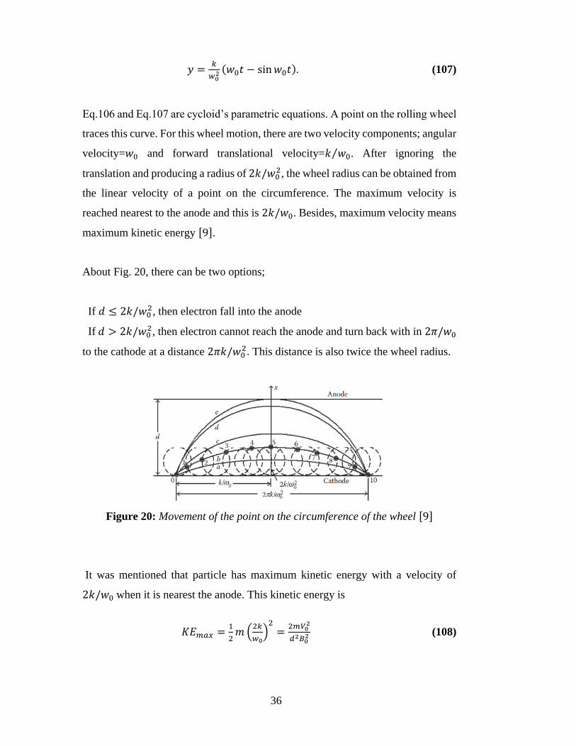
Eq.106 and Eq.107 are cycloid’s parametric equations. A point on the rolling wheel
traces this curve. For this wheel motion, there are two velocity components; angular
velocity=𝑤0 and forward translational velocity=𝑘 𝑤0⁄ . After ignoring the
translation and producing a radius of 2𝑘/𝑤02, the wheel radius can be obtained from
the linear velocity of a point on the circumference. The maximum velocity is
reached nearest to the anode and this is 2𝑘/𝑤0. Besides, maximum velocity means
maximum kinetic energy [9].
About Fig. 20, there can be two options;
If 𝑑 ≤ 2𝑘/𝑤02, then electron fall into the anode
If 𝑑 > 2𝑘/𝑤02, then electron cannot reach the anode and turn back with in 2𝜋/𝑤0
to the cathode at a distance 2𝜋𝑘/𝑤02. This distance is also twice the wheel radius.
Figure 20: Movement of the point on the circumference of the wheel [9]
It was mentioned that particle has maximum kinetic energy with a velocity of
2𝑘/𝑤0 when it is nearest the anode. This kinetic energy is
𝐾𝐸𝑚𝑎𝑥 =1
2𝑚 (
2𝑘
𝑤0)2=
2𝑚𝑉02
𝑑2𝐵02 (108)

37
This energy returns to electric field completely before the electrons turn back to
the cathode. Like it was said before this case is similar to case in Section 2.1.3
because there are only E and B fields.
AC field present: Let’s look what happens when AC field is applied.
𝛼𝑤02
𝑤2−𝑤02 =
1
2 and 𝑤 = 1.1𝑤0, then 𝛼 =
𝑉1
𝑉0= 0.105 (109)
Here we can see that the DC field magnitude (𝑉0) is much bigger than an AC field
magnitude (𝑉1). This situation is observed when a small ac signal is to be amplified
at the cost of a large applied dc source [9].
When above relations are considered, Eq.103 becomes
𝑥 =𝑘
𝑤02 (1 −
1
2cos𝑤0𝑡 −
1
2cos 1.1𝑤0𝑡)
=𝑘
𝑤02(1 − cos 0.05𝑤0𝑡 cos 1.05𝑤0𝑡)
=𝑘
𝑤02 −
𝑘
𝑤02 cos 0.05𝑤0𝑡 cos 1.05𝑤0𝑡 (110)
𝑦 =𝑘
𝑤02 [(𝑤0𝑡 −
1
2sin𝑤0𝑡) −
1
1.1
1
2sin 1.1𝑤0𝑡] (111)

38
Figure 21: Charged particle motion in the combined field [9]
Whit Eq.110 and Eq.111, the behavior of a charged particle in the combined field
is explained. Fig. 21 shows this motion. The motion of electron starts from the
cathode with a maximum distance (2𝑘/𝑤02). If electron does not reach the anode, it
oscillates by decreasing the amplitudes. This continuous until it rest at 𝑥 = 𝑘/𝑤02 at
𝑤0 = 10𝜋.
2.1.4.2 Cylindrical Coordinate System
In the previous section, I showed the electron path in the presence of E and B field.
In this section, I will explain the travelling path of electron in magnetron when there
are E field, B field and AC field. The radio frequency field (RF) is an alternating
current so this current generates an electromagnetic field which is called as a RF
field [10].There is a RF field inside all cavities and RF field changes the path of
electrons. With the help of shown paths in Fig. 22, we will understand the behavior
of electrons in magnetron.
Electron a: Tangential component of electric field arise from the RF field in the
magnetron. This tangential component prevents the tangential velocity of electron
when electron ‘a’ came to point 1. Hence, electron ‘a’ is geared down and transmits
its energy to the RF field. The magnetic field force on electron is decreased because
of this slowdown. Consequently, electron moves closer to the anode. Then, electron
‘a’ comes to the point 2, field polarity becomes reversed and electron ‘a’ is geared

39
down again and gives energy to the RF field. As a result, over again B field force
effect on electron ‘a’ decreases. In other words, every time E field polarity reverses
when electrons come at a proper position for interaction. In this way, electrons
spend a lot of time in interaction space and turn around the cathode many times
before they reach the anode.
Figure 22: (a) Electron paths in magnetron [9]
Electron b: Due to the location of electron ‘b’, RF field accelerates it so it gets
energy from RF field. Thus the magnetic force on it increases. As compared with
electron ’a’, ‘b’ spends much less time in interaction space. It turns back to the
cathode sooner than the electron return in absence of RF field. Given energy to the
RF field must be much more than the receiving energy. There are many electron
like ‘a’ and ‘b’. However, electron ‘b’ spends less time in the RF field when it is
compared with the electron ‘a’. Thus, ‘b’ takes energy from RF field but ‘a’ gives
much more of extracted energy to the RF field. Moreover, ‘a’ give energy again and
again while ‘b’ takes energy once or twice. This differences between electron ‘a’
and ‘b’ provide sustained oscillations.
Electron c: This electron also makes energy contribution to the RF field like as
electron ‘a’. However, tangential component of electron ‘c’ is not much powerful
by comparison with electron ’a’ so it cannot give much energy like ‘a’. However,
40
it runs across with the radial RF field component and it affects acceleration radially.
Magnetic field exerts force on electron ‘c’ strongly at this junction point and
electron ‘c’ returns to the cathode. For electron ‘d’, similarly magnetic field also
slows down it tangentially. Therefore, electron ‘d’ is grabbed by the favored
electrons which are in equilibrium position [9].
2.2 Electron Motion in Magnetron
In conventional (cylindrical) magnetron, there is a radially applied voltage (𝑉0)
between anode and cathode and magnetic field (𝐵0) is in the positive z direction.
Thus, �⃗� = 𝐸𝑟𝑎�̂� and �⃗� = 𝐵𝑧𝑎�̂�. About electrons, they have cycloidal motion in the
space of magnetron.
For given E and B field, Eq.82 and Eq.83 reduce to
𝑑2𝑟
𝑑𝑡2 − 𝑟𝑤2 =𝑒
𝑚(𝐸𝑟 − 𝐵𝑧𝑤𝑟) (112)
1
𝑟
𝑑
𝑑𝑡(𝑟2𝑤) =
𝑒
𝑚(𝐵𝑧
𝑑𝑟
𝑑𝑡) (113)
where 𝑤 = 𝑑∅ 𝑑𝑡⁄ .
Eq.113 can be written as
𝑑
𝑑𝑡(𝑟2𝑤) =
𝑒
𝑚𝑟𝐵𝑧
𝑑𝑟
𝑑𝑡=
1
2𝑤𝑐
𝑑
𝑑𝑡(𝑟2) (114)
where 𝑤𝑐 = (𝑒 𝑚⁄ )𝐵𝑧. And 𝑤𝑐 is the cyclotron angular frequency. If we integrate
the Eq.114, then we get
𝑟2𝑤 =1
2𝑤𝑐𝑟
2 + 𝑘1(𝑐𝑜𝑛𝑠𝑡𝑎𝑛𝑡) (115)

41
Let’s take cathode radius as 𝑎. Then the constant 𝑘1 is −𝑤𝑐𝑎2/2 when at 𝑟 = 𝑎
and 𝑤 = 0. So another formula for 𝑤 is
𝑤 =1
2𝑤𝑐 (1 −
𝑎2
𝑟2). (116)
The kinetic energy of the electron in the magnetron is
𝐾𝐸 =1
2𝑚𝑣2 = 𝑒𝑉 (117)
From Eq.117, we can write the electron velocity 𝑣 which has two components 𝑟
and ∅,
𝑣2 =2𝑒
𝑚𝑉 = 𝑣𝑟
2 + 𝑣∅2 = (
𝑑𝑟
𝑑𝑡)2+ (𝑟
𝑑∅
𝑑𝑡)2 (118)
Let’s inner radius of anode becomes 𝑏. When electron at 𝑟 = 𝑏, 𝑉 = 𝑉0 and
𝑑𝑟 𝑑𝑡 = 0⁄ which means when the electron just grazes the inner surface of anode,
Eq.116 becomes
(𝑑∅
𝑑𝑡) =
1
2𝑤𝑐 (1 −
𝑎2
𝑏2) (119)
Eq.119 can also be written as
𝑏2 (𝑑∅
𝑑𝑡)2=
2𝑒
𝑚𝑉0 (120)
When we substitute Eq.119 in Eq.120, we get
𝑏2 (1
2𝑤𝑐 (1 −
𝑎2
𝑏2))
2
=2𝑒
𝑚𝑉0 (121)

42
2.3 Hull Cutoff Equation for Magnetron
When we substitute 𝑤𝑐 equation in Eq.121 and do necessary arrangements, we find
following relations:
𝐵0𝑐 =(8𝑉0𝑚
𝑒)1/2
𝑏(1−𝑎2
𝑏2) (122)
𝑉0𝑐 =𝑒
8𝑚𝐵0
2𝑏2 (1 −𝑎2
𝑏2)2
(123)
For Eq.122 and Eq.123 we used 𝑤𝑐 = (𝑒 𝑚⁄ )𝐵𝑧. We call Eq.122 as the Hull cutoff
magnetic equation and result of this equation is the cutoff magnetic field (𝐵0𝑐). For
Eq.122, if 𝐵0 < 𝐵0𝑐 for a given voltage 𝑉0, then electron cannot arrive the anode.
Like for like-bases, name of the Eq.123 is the Hull cutoff voltage equation and if
we solve this equation we get the cutoff voltage (𝑉0𝑐). For Eq.123, if 𝑉0 < 𝑉0𝑐,
again electron cannot reach the anode [9].
2.4 Cyclotron Angular Frequency for an Electron
As mentioned earlier, the magnetic field and the cycloidal path of electron are
orthogonal to each other. The centrifugal force on electron equals to the pulling
force. So,
𝑚𝑣𝑡2
𝑅= 𝑒𝑣𝐵 (124)
Here 𝑅 is the path radius, 𝑣𝑡 is the tangential velocity.
The cyclotron angular frequency of the motion is
𝑤𝑐 =𝑣𝑡
𝑅=
𝑒𝐵
𝑚 (125)
One full revolution has the period which is shown below.

43
𝑇 =2𝜋
𝑤=
2𝜋𝑚
𝑒𝐵 (126)
In order to have oscillations in magnetron, construction must has an integral
multiple of 2𝜋 radians phase shift [9]. For the nth mode of the oscillation in an N
cavity magnetron, phase shift between two cavities is
∅𝑛 =2𝜋𝑚
𝑁 (127)
By adjusting the voltage of anode, it is possible to produce the oscillations.
Generally, magnetrons oscillates in 𝜋-mode. The necessary phase shift for this is
∅𝑛 = 𝜋 (128)
Fig. 23 illustrates the force lines of an eight-cavity magnetron in π-mode. Here,
successive descent and ascent of field in cavities can be thought as a travelling
wave. When field decelerates the electrons and each passing of electrons near the
cavities is occur, electrons give energy to the travelling wave [9].
Figure 23: Force lines of an 8-cavity magnetron in 𝜋-mode [9]

44
If the distance between the cavities is 𝐿, then the phase constant is
𝛽0 =2𝜋𝑛
𝑁𝐿 (129)
By using Maxwell’s equations and boundary conditions, we can obtain the solution
for ∅ component of the travelling wave electric field [9].Thus,
𝐸∅0 = 𝑗𝐸1𝑒𝑗(𝑤𝑡−𝛽0∅) (130)
The angular velocity of the travelling field is
𝑑∅
𝑑𝑡=
𝑤
𝛽0 (131)
As it understood from this relation, if the cyclotron frequency equals to the angular
frequency,
𝑤𝑐 = 𝛽0 (𝑑∅
𝑑𝑡) (132)
then field-electron interaction occurs and energy gets transferred.
2.5 Equivalent Circuit
Figure 24: Equivalent circuit for magnetrons resonator

45
Fig. 24 shows an equivalent circuit for magnetrons resonator. The values in the
figure are
𝑌𝑒 = the electronic admittance,
𝑉 = the RF voltage across the vane tips,
𝐶 = the capacitance at vane tips,
𝐿 = the inductance,
𝐺𝑟 = the conductance of the resonant,
𝐺𝐿 = the load conductance per resonator.
Each one of the resonators contains a similar resonant circuit like as in the Fig. 24
[9].
2.6 Quality Factor
For a resonant circuit,
the uncharged quality factor is shown as
𝑄𝑢𝑛 =𝑤0𝐶
𝐺𝑟 (133)
the external quality factor is shown as
𝑄𝑒𝑥𝑡 = 𝑤0𝐶
𝐺𝐿 (134)
the loaded quality factor is shown as
𝑄𝐿 = 𝑤0𝐶
𝐺𝐿+𝐺𝑟 (135)
In these three equations, angular resonant frequency (𝑤0) is equal to 2𝜋𝑓0.

46
2.7 Power and Efficiency
In magnetrons, there are two values of efficiency term. First one is the circuit
efficiency and this can be shown as
𝜂𝑐 =𝐺𝐿
𝐺𝐿+𝐺𝑟=
𝐺𝐿
𝐺𝑒𝑥𝑡=
1
(1+𝑄𝑒𝑥𝑡𝑄𝑢𝑛
) (136)
From Eq.136, we say that 𝜂𝑐 has its maximum value when 𝐺𝐿 ≫ 𝐺𝑟. This means
magnetron has heavy loading. For some cases, this does not desire because this
cause a sensitive tube in loading.
The second value of efficiency term is electronic efficiency which is
𝜂𝑒 =𝑃𝑔𝑒𝑛
𝑃𝑑𝑐 (137)
Here 𝑃𝑔𝑒𝑛 equals to 𝑃𝑑𝑐 − 𝑃𝑙𝑜𝑠𝑠 and it is the induced power of the RF into the anode
circuit. 𝑃𝑑𝑐 is power of dc supply and it is also 𝑉0𝐼0. 𝑃𝑙𝑜𝑠𝑠 is anode circuit’s power
lost. 𝑉0 is the anode voltage and 𝐼0 is used for the anode current. It is mentioned that
electrons generate the RF power and this equals to
𝑃𝑔𝑒𝑛 = 𝑉0𝐼0 − 𝑃𝑙𝑜𝑠𝑠 = 𝑉0𝐼0 − 𝐼0𝑚
2𝑒
𝑤02
𝛽2 +𝐸𝑚𝑎𝑥
2
𝐵𝑧2 =
1
2𝑁|𝑉|2
𝑤0𝐶
𝑄𝐿 (138)
In Eq.138, 𝑁 is resonator number, 𝑉 is the voltage in the resonator gap, 𝐸𝑚𝑎𝑥 is the
maximum value of electric field which is 𝑀1|𝑉|/𝐿, 𝛽 is the constant of phase, 𝛽𝑧 is
the magnetic flux density, 𝐿 is the distance between the vane tips and 𝑀1 is the gap
factor which is used for 𝜋-mode operation and 𝑀1 can be found by using the Eq.139.
𝑀1 = sin(𝛽𝑛𝛿 2⁄ )/(𝛽𝑛𝛿 2⁄ ) (139)
Here, for small 𝛿 values, 𝑀1 ≈ 1.
Eq.138 can be formed simply as

47
𝑃𝑔𝑒𝑛 =𝑁𝐿2
2𝑀12
𝑤0𝐶
𝑄𝐿𝐸𝑚𝑎𝑥
2 (140)
Then by using Eq.140, we can write electronic efficiency equation as
𝜂𝑒 =𝑃𝑔𝑒𝑛
𝑃𝑑𝑐=
(1−𝑚𝑤0
2
2𝑒𝑉0𝛽2)
(1+𝐼0𝑚𝑀1
2𝑄𝐿𝐵𝑧𝑒𝑁𝐿2𝑤0𝐶
)
(141)
In this chapter we explained the physics behind of magnetron. Finally we achieved
the general power equation (Eq.140) and explained the parameters in this equation.
In next chapter, we will come to actual work and show the derivations of some of
these parameters and rewrite the generated power equation more detailed form. In
Chapter 3, our aim is to analyze the effects of some critical parameters on power
generation in magnetron.

48

49
CHAPTER 3
PARAMETERS WHICH AFFECT THE GENERATED POWER
We talked about the generated power in Chapter 2. We showed that electrons
generate the RF power in Eq.140 which equals to
𝑃𝑔𝑒𝑛 =𝑁𝐿2
2𝑀12
𝑤0𝐶
𝑄𝐿𝐸𝑚𝑎𝑥
2
Here,
𝑁 = resonator number,
𝐿 = the distance between the vane tips,
𝑀1 = gap factor,
𝑤0 = angular resonant frequency,
𝐶 = the capacitance at vane tips,
𝑄𝐿 = the loaded quality factor,
𝐸𝑚𝑎𝑥 = the maximum value of electric field.
In this chapter we will analyze that how some of these parameters change the
generated power.
3.1 Derivations of Some Important Parameters
In power equation, some parameters must be written in different forms to observe
exact effects on power. Therefore, firstly we should get the bottom of these
parameters.
50
3.1.1 Electric Field
We mentioned that negatively charged cathode and positively charged anode block
cause an electric field between each other. This radial field was derived in Eq.40
which is
𝐸𝑟 = −𝜕𝑉
𝜕𝑟= −𝑉0
1
𝑟 ln 𝑏/𝑎
𝐸∅ = 𝐸𝑧 = 0
Here 𝑉0 is applied voltage, 𝑎 is cathode radius and 𝑏 is anode radius. Maximum
value of electric field can be observed on the cathode surface. The 𝐸𝑚𝑎𝑥 can be
written as
𝐸𝑚𝑎𝑥 = −𝑉01
𝑎 ln 𝑏/𝑎 (142)
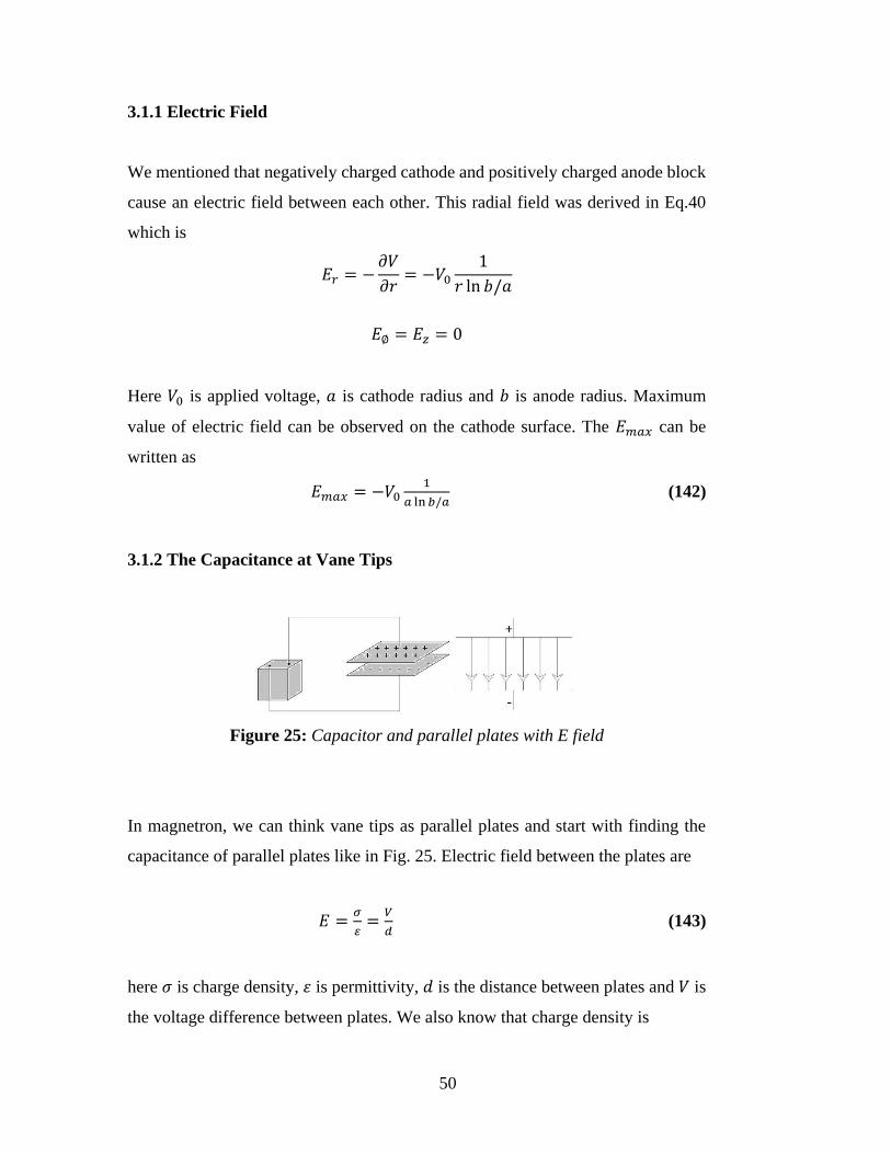
3.1.2 The Capacitance at Vane Tips
Figure 25: Capacitor and parallel plates with E field
In magnetron, we can think vane tips as parallel plates and start with finding the
capacitance of parallel plates like in Fig. 25. Electric field between the plates are
𝐸 =𝜎
=𝑉
𝑑 (143)
here 𝜎 is charge density, 휀 is permittivity, 𝑑 is the distance between plates and 𝑉 is
the voltage difference between plates. We also know that charge density is

51
𝜎 =𝑐ℎ𝑎𝑟𝑔𝑒 𝑜𝑛 𝑝𝑙𝑎𝑡𝑒
𝑎𝑟𝑒𝑎 𝑜𝑓 𝑝𝑙𝑎𝑡𝑒=
𝑄
𝐴 (144)
If we use the capacitance definition, we obtain
𝐶 =𝑆𝑡𝑜𝑟𝑒𝑑 𝑐ℎ𝑎𝑟𝑔𝑒 𝑜𝑛 𝑝𝑙𝑎𝑡𝑒
𝐴𝑝𝑝𝑙𝑖𝑒𝑑 𝑣𝑜𝑙𝑡𝑎𝑔𝑒=
𝑄
𝑉=
𝑄
𝐸𝑑=
𝑄
𝜎𝑑=
𝐴
𝑑=
𝑘 0𝐴
𝑑 (145)
here 휀0 is space permittivity and equals to 8.854 × 10⁻¹²𝐹𝑎𝑟𝑎𝑑/𝑚𝑒𝑡𝑒𝑟 and 𝑘 is
relative permittivity for dielectric material between the plates and equals to 1 for
air.
3.1.3 Angular Resonant Frequency
Angular resonant frequency, 𝑤0, equals to 2𝜋𝑓0. Here 𝑓0 is the cavity resonant
frequency. We multiplies 𝑓0 with 2𝜋 because one revolution is equal to 2𝜋. Fig.26
shows simple cavity resonant system and we use Eq. 146 to find the value of the
cavity resonant frequency which is
Figure 26: Cavity resonant
𝑓0 =𝑣𝑠
2𝜋√
𝐴
𝑉𝐿 (146)
52
here 𝑣𝑠 is the speed of sound. In dry air, speed of sound is approximately 340 m/s.
However, we use Eq. 147 for any cavity
𝑣𝑠𝑜𝑢𝑛𝑑 = √𝛾𝑅𝑇
𝑀 (147)
here 𝛾 is adiabatic constant and it is about the gas characteristic, 𝑅 is gas constant
(8.314 𝐽 𝑚𝑜𝑙. 𝐾⁄ ), 𝑀 is molecular mass of gas and 𝑇 is temperature. For air 𝛾 = 1.4
and 𝑀 = 28.95 𝑔/𝑚𝑜𝑙.
Eq. 146 is Helmholtz resonance frequency formula. To derive this formula, let’s
look at Fig.27
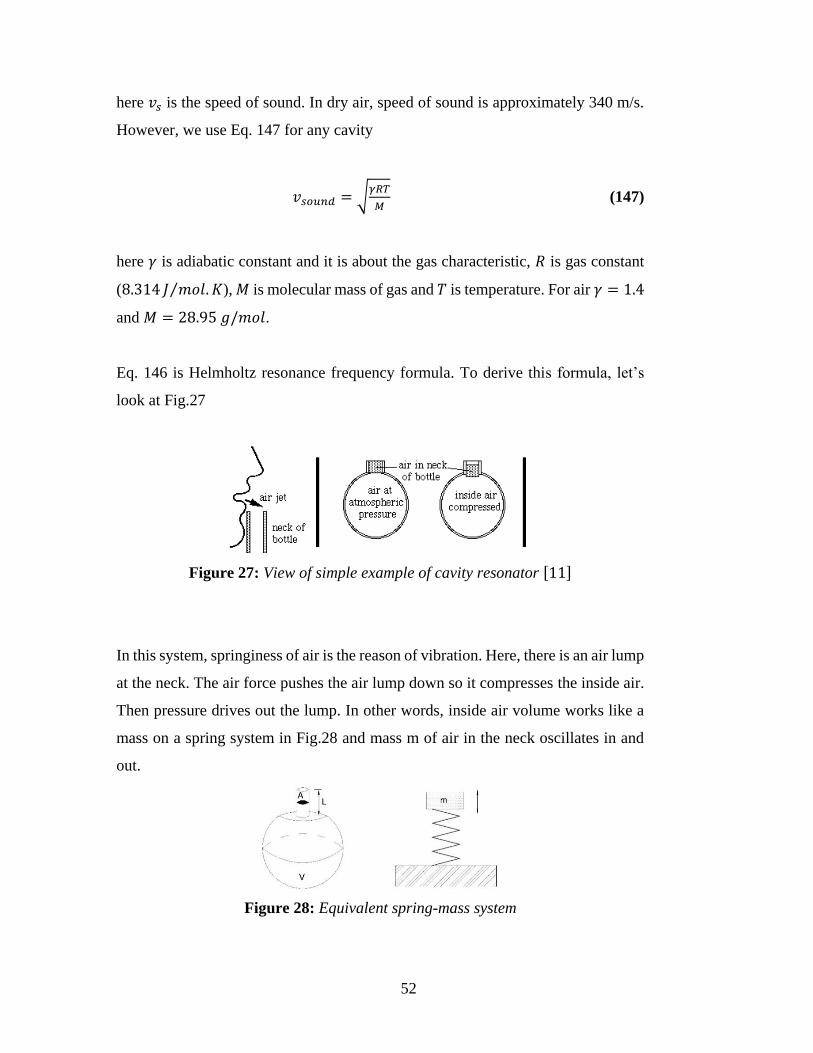
Figure 27: View of simple example of cavity resonator [11]
In this system, springiness of air is the reason of vibration. Here, there is an air lump
at the neck. The air force pushes the air lump down so it compresses the inside air.
Then pressure drives out the lump. In other words, inside air volume works like a
mass on a spring system in Fig.28 and mass m of air in the neck oscillates in and
out.
Figure 28: Equivalent spring-mass system

53
For spring-mass system, angular frequency formula with spring constant, k, is
𝑤 = √𝑘
𝑚 (148)
Air lump mass can be calculated with the density of the air (𝜌) and it is found as
𝑚 = 𝜌𝐿𝐴 (149)
here 𝐿 is the neck length and 𝐴 is the opening area of the neck. The change of
resonator volume is
𝑑𝑉 = −𝐴𝑑𝑥 (150)
here 𝑑𝑥 is the air lump displacement and the volume decrease causes minus sign.
The bulk modulus is the other parameter for derivation of Eq. 146. The bulk
modulus is the ability of a material to resist deformation in terms of volume change,
when subject to compression under pressure. The relation is
𝐾 = −𝑉𝑑𝑃
𝑑𝑉 (151)
here 𝐾 the bulk modulus (𝑁 𝑚2⁄ 𝑜𝑟 𝑃𝑎), 𝑑𝑃 is the change in applied pressure, 𝑉
is volume of the system and 𝑑𝑉 is the change in system volume. From Eq. 151, we
can write
𝑑𝑃 = 𝐾 (−𝑑𝑉
𝑉) (152)
If we insert Eq. 150 into Eq. 152 we obtain
54
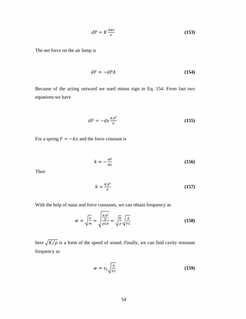
𝑑𝑃 = 𝐾𝐴𝑑𝑥
𝑉 (153)
The net force on the air lump is
𝑑𝐹 = −𝑑𝑃𝐴 (154)
Because of the acting outward we used minus sign in Eq. 154. From last two
equations we have
𝑑𝐹 = −𝑑𝑥𝐾𝐴2
𝑉 (155)
For a spring 𝐹 = −𝑘𝑥 and the force constant is
𝑘 = −𝑑𝐹
𝑑𝑥 (156)
Then
𝑘 =𝐾𝐴2
𝑉 (157)
With the help of mass and force constants, we can obtain frequency as
𝑤 = √𝑘
𝑚= √
𝐾𝐴2
𝑉
𝜌𝐿𝐴= √
𝐾
𝜌√
𝐴
𝑉𝐿 (158)
here √𝐾 𝜌⁄ is a form of the speed of sound. Finally, we can find cavity resonant
frequency as
𝑤 = 𝑣𝑠√𝐴
𝑉𝐿 (159)

55
Frequency formula shows that, smaller opening gives lower frequency since air can
rush in and out slower. Besides, smaller volume gives higher frequency because
less air must move out to relieve a given pressure excess. Lastly, shorter neck gives
higher frequency by reason of there is less resistance to air moving in and out [12].
3.1.4 Electrical Conductivity
Conductivity is about current flow through a material. In more detail, for a given
electric field in a material, a lower conductivity material will produce less current
flow than a high conductivity material.
Loss in power and conductivity are proportional. We use ‘lossless’ word for a zero
conductivity material which are air, vacuum etc. If conductivity is bigger than zero,
‘loosy’ word can use for these materials that are salt water, silicon etc. Finally, some
materials such as metals, copper, silver, etc. are named as ‘conductors’. Conductors
have far greater conductivity which is approximately infinite. Table 1 contains
conductivity value and classification of some materials [13].

56
Table 1: Conductivity values of different materials [13]
Material 𝛔 [𝐒/𝐦] Classification
Silver 6.3 x 10⁷ Conductor
Copper 6.0 x 10⁷ Conductor
Aluminum 3.5 x 10⁷ Conductor
Tungsten 1.8 x 10⁷ Conductor
Nickel 1.4 x 10⁷ Conductor
Iron 1.0 x 10⁷ Conductor
Mercury 1.0 x 10⁶ Conductor
Carbon 2.0 x 10³ Lossy
Sea Water 4.8 Lossy
Germanium 2.17 Lossy
Silicon 1.6 x 10⁻³ Lossy
Glass ~10-12 Lossless
Rubber ~10-14 Lossless
Air ~10-15 Lossless
Teflon ~10-24 Lossless
Vacuum 0 Lossless

57
To derive conductivity we should know that conductivity is the inverse of resistivity
of material. Well then, what is resistivity exactly? The answer starts with Fig.29.
Figure 29: Simple circuit
𝑅 =𝑉
𝐼 (160)
Here 𝑉 is potential in volt, 𝐼 is current in ampere and 𝑅 is resistance. If we increase
voltage, this increases the current and 𝑉/𝐼 ratio stays same so increase in voltage
never changes the resistance. In other words, resistance has a constant value and it
changes only if we changes resistor material, makeup, size or dimensions. To
understand better, the bigger view of resistor is shown in Fig.30.
Figure 30: View of resistor
Here 𝜌 is resistivity and specific for material. Resistance formula is
𝑅 = 𝜌𝐿
𝐴 (161)

58
Resistivity gives an idea of how much something naturally resists current and
conductivity tells how much something naturally allows current. I mentioned that
inverse of resistivity gives conductivity.
Then the other form of resistance is
𝑅 =𝐿
𝜎𝐴=
𝐿
𝜎𝜋𝑟2 (162)
In Eq. 162, 𝑟 is radius of resistor. Here 𝑅 is DC resistance for a conductor. At DC,
charge carriers are equally separeted through the whole cross section area of
resistor.
With the increase in frequency, the magnetic field at the inductor center increases
and this causes an increase on the reactance near the center of resistor. Therefore,
charges in resistor moves to edges from the center. Thus, the current density
decreases at the center while it increases at the edges. This situation is explained as
‘skin effect’. Besides, ‘skin depth’ is the depth into conductor where the current
density falls to 37% of its surface value. The skin depth formula is
𝛿 =1
√𝜋𝑓𝜇𝜎 (163)
where 𝜇 is permeability, 𝑓 is frequency and 𝜎 is conductivity of the material.
Resistance and frequency are proportional to each other and skin depth dependent
resistance is named as an AC resistance. Eq. 164 shows a formula for an AC
resistance approximately.
𝑅𝑎𝑐 =𝐿
𝜎𝐴𝑎𝑐𝑡𝑖𝑣𝑒 (164)
here 𝐴𝑎𝑐𝑡𝑖𝑣𝑒 is the skin depth area on the conductor and equals to 2𝜋𝑟𝛿 . Then Eq.
164 becomes

59
𝑅𝑎𝑐 =𝐿
𝜎2𝜋𝑟𝛿=
𝐿
2𝑟√
𝑓𝜇
𝜋𝜎= (𝑅𝑑𝑐)
𝑟
2𝛿 (165)
As seen in Eq. 165, AC resistance proportionally changes with the square root of
frequency [14].
3.2 Observations of Change in Power about Effects of Some Parameters
We did our observations by taking generated power formula in Eq. 166 and a
magnetron like as in Fig.31 into consideration.
𝑃𝑔𝑒𝑛 =𝑁𝐿2
2𝑀12 (𝑣𝑠√
𝐴
𝑉𝐿′) (𝑘 0𝐴′
𝑑)
1
𝑄𝐿(−𝑉0
1
𝑎 ln(𝑏 𝑎⁄ ))
2 (166)
Here as mentioned before, 𝑁 is cavity number, 𝐿 is distance between vane tips, 𝑀1
is gap factor and 𝑄𝐿 is loaded quality factor. In this formula we use Eq. 149 instead
of angular resonant frequency term (𝑤0) so 𝐿′ is length of opening part of cavities
in this equation. Besides, instead of the capacitance at vane tips term (𝐶), the
capacitance form in Eq. 145 is used. Lastly, we use more detailed form of 𝐸𝑚𝑎𝑥
shown in Eq. 142.
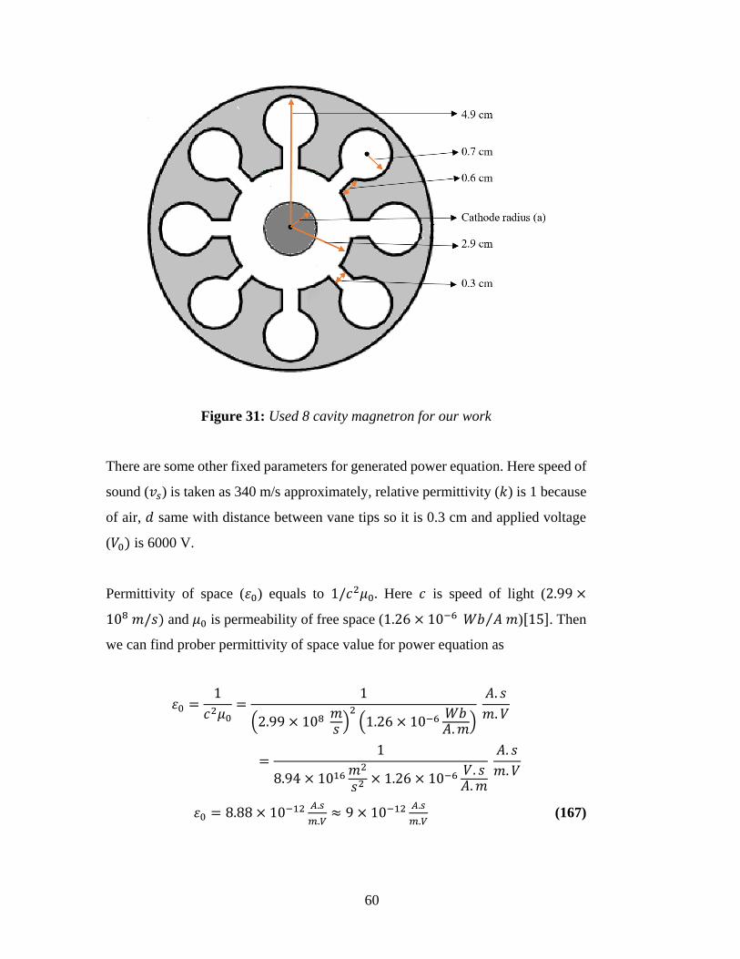
For used magnetron as seen in Fig.31, distance between the vane tips (𝐿) is 0.3 cm,
anode radius (𝑏) is 2.9 cm, length of the opening part of the cavities (𝐿′) is 0.6 cm,
radius of cavities is 0,7 cm and the distance between magnetron center and the
outermost point of cavity surface from the center is 4.9 cm. Cathode radius (𝑎), gap
factor (𝑀1), the loaded quality factor (𝑄𝐿) and cavity number (𝑁) will change
according to our calculations.
60
Figure 31: Used 8 cavity magnetron for our work
There are some other fixed parameters for generated power equation. Here speed of
sound (𝑣𝑠) is taken as 340 m/s approximately, relative permittivity (𝑘) is 1 because
of air, 𝑑 same with distance between vane tips so it is 0.3 cm and applied voltage
(𝑉0) is 6000 V.
Permittivity of space (휀0) equals to 1/𝑐2𝜇0. Here 𝑐 is speed of light (2.99 ×
108 𝑚/𝑠) and 𝜇0 is permeability of free space (1.26 × 10⁻⁶ 𝑊𝑏 𝐴 𝑚⁄ )[15]. Then
we can find prober permittivity of space value for power equation as
휀0 =1
𝑐2𝜇0=
1
(2.99 × 10⁸ 𝑚𝑠
)2
(1.26 × 10⁻⁶ 𝑊𝑏𝐴. 𝑚
)
𝐴. 𝑠
𝑚. 𝑉
=1
8.94 × 10¹⁶ 𝑚2
𝑠2 × 1.26 × 10−6 𝑉. 𝑠𝐴. 𝑚
𝐴. 𝑠
𝑚. 𝑉
휀0 = 8.88 × 10⁻¹² 𝐴.𝑠
𝑚.𝑉≈ 9 × 10⁻¹² 𝐴.𝑠
𝑚.𝑉 (167)

61
To calculate volume of the cavity (𝑉), we use 𝜋𝑟2ℎ formula. Here ℎ is height of
magnetron. In Fig.31, one dimensional view of magnetron is seen. However, it also
has a height and we take it as 5 cm. Then cavity volume is
𝑉 = 𝜋 × 𝑟2 × ℎ = 𝜋 × (0.7 𝑐𝑚)2 × 5 𝑐𝑚 = 7.697 𝑐𝑚3 (168)
The area of opening part of cavity (𝐴) is calculated by multiplying height with the
distance between the vane tips. Then opening part area is
𝐴 = ℎ × 𝐿 = 5 𝑐𝑚 × 0.3 𝑐𝑚 = 1.5 𝑐𝑚2 (169)
We used 𝐴′ term for plate area in Eq. 145 and it equals
𝐴′ = ℎ × 𝐿′ = 5 𝑐𝑚 × 0.6 𝑐𝑚 = 3 𝑐𝑚2 (170)
3.2.1 Effect of Cavity Number on Generated Power
In this section, we observed that how generated power changes with respect to
cavity number. We worked with Eq. 166 and we changed the cavity number from
4 to 12. Moreover, increment of resonant number was 2 because we should have
even number of cavities in order that side-by-side segments have opposite poles.
This was also shown in Fig.8. For a true observation, we kept fixed the other
variables in the formula. The values of parameters which we used are shown in
Table 2.

62
Table 2: Values of variables for cavity number-power graph
Variable Value Variable Value
𝑳 0.3 cm 𝜺𝟎 9x10-12 A.s/m.V
𝑴𝟏 1 𝑨′ 3 cm2
𝒗𝒔 340 m/s 𝒅 0.3 cm
𝑨 1.5 cm2 𝑸𝑳 10
𝑽 7.697 cm3 𝑽𝟎 6000 V
𝑳′ 0.6 cm 𝒂 1.6 cm
𝒌 1 𝒃 2.9 cm
In graph, we used the data in Table 2 and created the cavity number versus
generated power graph. This is shown in Fig.32 and it is understood that resonator
number and generated power are directly proportional.
Figure 32: Cavity Number versus Generated Power Graph

63
3.2.2 Effect of Gap Factor on Generated Power
After resonator number, we analyzed the effects of gap factor on generated power.
We again used Eq. 166 and we took the gap factor values from 0.5 to 1.5. Moreover,
increment of gap factor values was 0.01 in order to obtain more smoothly graph.
For an accurate observation, we kept some variables fixed. The used variables can
be seen in Table 3.
Table 3: Values of variables for gap factor-power graph
Variable Value Variable Value
𝑵 8 𝜺𝟎 9x10-12 A.s/m.V
𝑳 0.3 cm 𝑨′ 3 cm2
𝒗𝒔 340 m/s 𝒅 0.3 cm
𝑨 1.5 cm2 𝑸𝑳 10
𝑽 7.697 cm3 𝑽𝟎 6000 V
𝑳′ 0.6 cm 𝒂 1.6 cm
𝒌 1 𝒃 2.9 cm
The curve of gap factor versus generated power is shown in Fig.33. As seen, when
we increase the gap factor value, generated power decreases exponentially.

64
Figure 33: Gap Factor versus Generated Power Graph
After that, we took the first and second derivatives of power with respect to gap
factor. The first derivative of Eq. 166 is
𝑃𝑔𝑒𝑛′ (𝑀1) = − (
𝑁𝐿2
𝑀13 ) (𝑣𝑠√
𝐴
𝑉𝐿′) (𝑘 0𝐴′
𝑑)
1
𝑄𝐿(−𝑉0
1
𝑎 ln(𝑏 𝑎⁄ ))
2 (171)
and the second derivative of Eq. 166 is
𝑃𝑔𝑒𝑛′′ (𝑀1) = (
3𝑁𝐿2
𝑀14 ) (𝑣𝑠√
𝐴
𝑉𝐿′) (𝑘 0𝐴′
𝑑)
1
𝑄𝐿(−𝑉0
1
𝑎 ln(𝑏 𝑎⁄ ))
2 (172)
From Eq. 171 and Eq. 172 we formed Fig.34 and Fig.35. In graph of first derivative,
we saw that maximum changes are observed from 0.5 to 0.8. Moreover, it reached
the saturating point at 1.5. About Fig.35, our aim was to see whether there is a
maximum and a minimum points or not. If there was a peak in this graph, we would
choose peak value as an optimized gap factor value but there was not.

65
Figure 34: Gap Factor versus 1st Derivative of Power Graph
Figure 35: Gap Factor versus 2nd Derivative of Power Graph

66
3.2.3 Effect of Loaded Quality Factor on Generated Power
Thirdly, we observed the changes in generated power when loaded quality factor
value is changed. We used the loaded quality factor values between 5 and 15 and
again we increased the value by 0.01 because of the same reasons before. The fixed
values for Eq. 166 are listed in Table 4.
Table 4: Values of variables for loaded quality factor-power graph
Variable Value Variable Value
𝑵 8 𝒌 1
𝑳 0.3 cm 𝜺𝟎 9x10-12 A.s/m.V
𝑴𝟏 1 𝑨′ 3 cm2
𝒗𝒔 340 m/s 𝒅 0.3 cm
𝑨 1.5 cm2 𝑽𝟎 6000 V
𝑽 7.697 cm3 𝒂 1.6 cm
𝑳′ 0.6 cm 𝒃 2.9 cm
We got the Fig.36 which shows the power changes according to loaded quality
factor. It is seen that if we increase the loaded quality factor value, the generated
power decreases exponentially.

67
Figure 36: Loaded Quality Factor versus Generated Power Graph
Then we looked the derivatives of power with respect to loaded quality factor. After
all, we obtained Eq. 173 for first derivative and Eq. 174 for second derivative.
𝑃𝑔𝑒𝑛′ (𝑄𝐿) = −
1
𝑄𝐿2 (
𝑁𝐿2
2𝑀12) (𝑣𝑠√
𝐴
𝑉𝐿′) (𝑘 0𝐴′
𝑑) (−𝑉0
1
𝑎 ln(𝑏 𝑎⁄ ))
2 (173)
𝑃𝑔𝑒𝑛′′ (𝑄𝐿) =
1
𝑄𝐿3 (
𝑁𝐿2
𝑀12 ) (𝑣𝑠√
𝐴
𝑉𝐿′) (𝑘 0𝐴′
𝑑) (−𝑉0
1
𝑎 ln(𝑏 𝑎⁄ ))
2 (174)
Thereafter, with the help of last two equations we obtain Fig. 37 and Fig. 38 for
derivatives of generated power. In the graph of first derivative, we observed the
maximum change gap as between 5 and 8. Moreover, from Fig.37 it is seen that 15
is saturating point for the loaded quality factor. Moreover, the graph of second
derivative again did not give us a peak so there is not exact loaded quality factor
value.
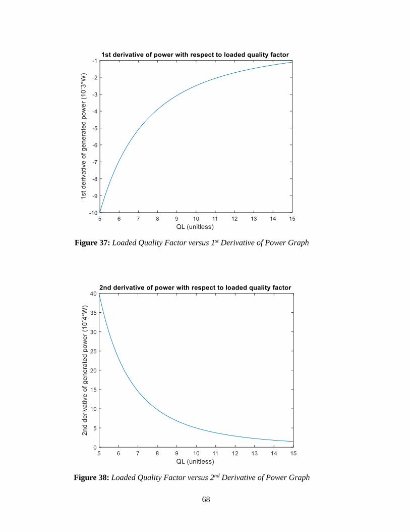
68
Figure 37: Loaded Quality Factor versus 1st Derivative of Power Graph
Figure 38: Loaded Quality Factor versus 2nd Derivative of Power Graph

69
3.2.4 Effect of Cathode Radius on Generated Power
After loaded quality factor, we looked for the effects of cathode radius. We changed
the cathode radius value from 1 cm to 2.2 cm in Eq. 166. Again to have a smooth
graphic, we used increments as 0.01 cm. The unchanged values for this part are
shown in Table 5.
Table 5: Values of variables for cathode radius-power graph
Variable Value Variable Value
𝑵 8 𝒌 1
𝑳 0.3 cm 𝜺𝟎 9x10-12 A.s/m.V
𝑴𝟏 1 𝑨′ 3 cm2
𝒗𝒔 340 m/s 𝒅 0.3 cm
𝑨 1.5 cm2 𝑸𝑳 10
𝑽 7.697 cm3 𝑽𝟎 6000 V
𝑳′ 0.6 cm 𝒃 2.9 cm
With the help of the values in Table 5, we obtained Fig. 39 which is a graphic of
cathode radius versus generated power. Here, we see an exponential increase in
power so if we use bigger cathode, we get larger power.

70
Figure 39: Cathode Radius versus Generated Power Graph
Then we took the derivative of generated power with respect to cathode radius. The
first derivative is
𝑃𝑔𝑒𝑛′ (𝑎) =
𝑁𝐿2
2𝑀12 (𝑣𝑠√
𝐴
𝑉𝐿′) (𝑘 0𝐴′
𝑑)
1
𝑄𝐿(−
2𝑉02(ln
𝑏
𝑎−1)
(ln𝑏
𝑎)
3𝑎3
) (175)
𝑃𝑔𝑒𝑛′′ (𝑎) =
𝑁𝐿2
2𝑀12 (𝑣𝑠√
𝐴
𝑉𝐿′) (𝑘 0𝐴′
𝑑)
1
𝑄𝐿(
2𝑉02(3(ln
𝑏
𝑎)
2−5 ln(
𝑏
𝑎)+3)
(ln𝑏
𝑎)
4𝑎4
) (176)
After that, we formed the graph of cathode radius versus the first derivative of
generated power as in Fig. 40 and the second derivative of generated power as in
Fig. 41.

71
Figure 40: Cathode Radius versus 1st Derivative of Power Graph
In the graph of first derivative, maximum change occurred between 1.8 cm and 2.2
cm and saturation point did not observed. Moreover, There was not any peak point
in the graph of second derivative of power with respect to cathode radius like as
previous second derivative graphs.
Figure 41: Cathode Radius versus 2nd Derivative of Power Graph

72
3.2.5 Effect of Angular Resonant Frequency on Generated Power
In this section again we worked with Eq.140 which is
𝑃𝑔𝑒𝑛 =𝑁𝐿2
2𝑀12
𝑤0𝐶
𝑄𝐿𝐸𝑚𝑎𝑥
2
Firstly, we fixed some parameters. We chose cavity number 𝑁 as 8, gap factor 𝑀1
as 1 and cathode radius 𝑎 as 2 cm. Before we mentioned that distance between the
vane tips (𝐿) is 0,3 cm for our magnetron design. We showed the maximum electric
field in Eq.142 as
𝐸𝑚𝑎𝑥 = −𝑉0
1
𝑎 ln 𝑏/𝑎
Here, anode radius 𝑏 was 2.9 cm and voltage value was 6000 volt. We just want to
observe how the generated power changes with frequency so we can also fixed
𝐶 𝑄𝐿⁄ term. The took loaded quality factor as 10 and the capacitance at vane tips
constant is
𝐶 =𝑘 0𝐴′
𝑑=
1×(9×10−10 𝐴.𝑠
𝑐𝑚.𝑉)×(1.3 𝑐𝑚2)
0.3 𝑐𝑚 𝐴.𝑠
𝑉= 39 × 10−10 𝐴.𝑠
𝑉 (177)
Then our equation became
𝑃𝑔𝑒𝑛 =8 × (0.3 𝑐𝑚)2
2 × 12× 𝑤0 ×
(39 × 10−10 𝐴. 𝑠𝑉
)
10
× (−6000 𝑉 ×1
(2 𝑐𝑚) × ln2.9 𝑐𝑚2 𝑐𝑚
)
2
𝑃𝑔𝑒𝑛 = 𝑤0 × 0.68 × 10−2 𝑊. 𝑠 (178)
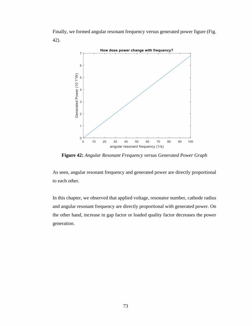
73
Finally, we formed angular resonant frequency versus generated power figure (Fig.
42).
Figure 42: Angular Resonant Frequency versus Generated Power Graph
As seen, angular resonant frequency and generated power are directly proportional
to each other.
In this chapter, we observed that applied voltage, resonator number, cathode radius
and angular resonant frequency are directly proportional with generated power. On
the other hand, increase in gap factor or loaded quality factor decreases the power
generation.

74

75
CHAPTER 4
CONCLUSION & DISCUSSION
Medical X-ray sources, radiotherapy, microwave heating, industrial heating,
communication, warfare, cargo scanning and radar are some of the areas that
used magnetron. In short, the usage area of magnetron is very wide. This causes
that producing magnetrons with different types, geometries, sizes and power is
necessary. The studies on magnetron started in 1912 and since then, it has been
being improved a lot [5]. With the effect of changing and proceeding technology,
studies on magnetron will continue to increase.
In this study, we have mentioned construction, working principle and0 critical
parameters of magnetrons. Magnetrons are crossed-field devices and generate
microwaves. The frequency range of microwaves is about between 300 MHz and
300 GHz. Its small size, light weight, low-cost and working with high efficiency
make magnetrons most promising and popular high power microwave device.
Simply, in the middle of it there is a cathode part, then there is an interaction
space roundly and it ends up with an anode part which surrounds the interaction
space (Fig. 5). All system starts at cathode. Electrons are spread from cathode
and they are kept in the space with the help of electric, magnetic and AC fields.
Electrons move directly from cathode to anode with the help of electric field
which is in radial direction. Then, magnetic field which is perpendicular to
electric field bends them. After all, we want to have very long electron path so
electrons should stay in space very long time in order to have better and more
efficient microwave generation. Therefore, electrons should have cycloidal
motion in the interaction space of cylindrical magnetron and this motion is
shown in Figure 43.
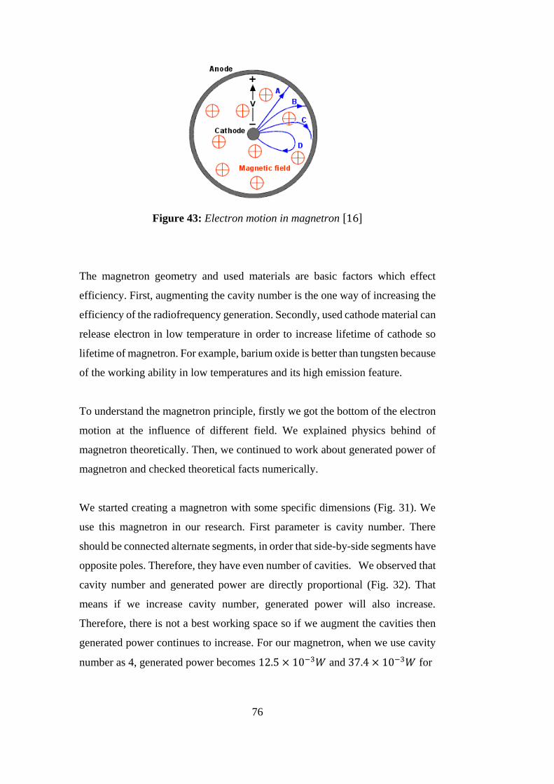
76
Figure 43: Electron motion in magnetron [16]
The magnetron geometry and used materials are basic factors which effect
efficiency. First, augmenting the cavity number is the one way of increasing the
efficiency of the radiofrequency generation. Secondly, used cathode material can
release electron in low temperature in order to increase lifetime of cathode so
lifetime of magnetron. For example, barium oxide is better than tungsten because
of the working ability in low temperatures and its high emission feature.
To understand the magnetron principle, firstly we got the bottom of the electron
motion at the influence of different field. We explained physics behind of
magnetron theoretically. Then, we continued to work about generated power of
magnetron and checked theoretical facts numerically.
We started creating a magnetron with some specific dimensions (Fig. 31). We
use this magnetron in our research. First parameter is cavity number. There
should be connected alternate segments, in order that side-by-side segments have
opposite poles. Therefore, they have even number of cavities. We observed that
cavity number and generated power are directly proportional (Fig. 32). That
means if we increase cavity number, generated power will also increase.
Therefore, there is not a best working space so if we augment the cavities then
generated power continues to increase. For our magnetron, when we use cavity
number as 4, generated power becomes 12.5 × 10⁻³𝑊 and 37.4 × 10⁻³𝑊 for

77
12-cavity magnetron. Second one is the gap factor. Gap factor is a unitless
parameter used for a specific operation mode which causes the greatest output
power. We changed the gap factor value and drew a curve (Fig. 33). Here, power
and gap factor were inversely proportional. In other words, power decreases
exponentially when we increase the gap factor value. For used magnetron,
generated power was 9.99 × 10⁻²𝑊 if gap factor was 0.5 and 1.11 × 10⁻²𝑊
for gap factor value of 1.5. Then, we took the derivative of power with respect
to gap factor in order to find the fastest change (Fig. 34). In graph of first
derivative, we saw that maximum changes are observed from 0.5 to 0.8. When
gap factor equaled to 0.8, power was 3.9 × 10⁻²𝑊. In other words, average
change was about 2.03 × 10⁻²𝑊 for each 0.1 increase in gap factor until the
value of 0.8. However, after 0.8, for each 0.1 increase, the average change
became 0.4 × 10⁻²𝑊. Moreover, it reached the saturating point at 1.5 so after
this value increase in gap factor do not change power effectively (Fig. 34).
Lastly, we looked the second derivative of power with respect to gap factor. Our
aim was to see whether there is a maximum and a minimum points or not. If
there was a peak in this graph, we would choose peak value as an optimized gap
factor value but there was not (Fig. 35). The loaded quality factor is the third
parameter. When we increase the loaded quality factor value, we observed an
exponential decrease in generated power (Fig. 36). We got 49.9 × 10⁻³𝑊
power when the loaded quality factor was 5 and 16.6 × 10⁻³𝑊 at 15. Then we
looked first derivative graph as before and determined the maximum change gap
as between 5 and 8 (Fig. 37). Between 5 and 8, the average change was about
6.2 × 10⁻³𝑊 and after that it became 2.1 × 10⁻³𝑊 approximately. In other
words, after the value of 8, the power change is not too much and after the value
of 15, it does not change. Therefore, 15 is saturating point for the loaded quality
factor (Fig. 37). Moreover, second derivative again did not give us a peak so
there is not exact loaded quality factor value (Fig. 38). If we make a comparison
between gap factor graphs and loaded quality factor graphs, change in gap factor
affects the power more. For example, when we doubled gap factor, generated
power decrease became 7.7 × 10⁻²𝑊 and the loaded quality factor is doubled,
78
change in generated power was 2,4 × 10⁻²𝑊. This also seen in theoretical
power equation (Eq. 166). As seen in equation, gap factor used in square form.
Fourth parameter is cathode radius. This time figure gave as an exponential
increase on generated power when we used larger cathode (Fig. 39). When
cathode radius was 1 cm, power generation became 19,9 × 10⁻³𝑊 and 61.2 ×
10−3𝑊 if it was 2.2 cm. In the graph of first derivative, maximum change
occurred between 1.8 cm and 2.2 cm (Fig. 40). The average change was about
1.35 × 10⁻³𝑊 between 1 cm and 1.8 cm while it was 7.63 × 10⁻³𝑊
approximately between 1.8 cm and 2.2 cm. When we doubled the cathode radius,
change in power became 2.1 × 10⁻²𝑊. Therefore, by looking our magnetron,
we can say that cathode radius changes are less effective on power when it is
compared with gap factor and it has almost same effect on power generation with
loaded quality factor. Moreover, in derivative graph, saturation point did not
observed (Fig. 40). There was not any peak point in the graph of second
derivative of power with respect to cathode radius like as previous second
derivative graphs (Fig. 41). Angular resonant frequency is the last parameter that
we examine. We used constant values for variables in power equation except
frequency and we came up to a linear equation (Eq. 178). Then, we obtained a
power versus frequency figure which shows they are directly proportional to
each other (Fig. 42). Therefore, there is not any working space. If we continue
to increase frequency, generated power is also increases.
Thus far, we told about what we did but we also have some plans in the matter
of what we do next and there are some aims and matters that can be clarified.
Firstly, we can work with 2D and then 3D simulations of magnetron that have
different shapes or sizes and learn the working principle and effects of different
parameters visually so more clearly. Before we said that barium oxide cathode
is better than tungsten one. Then secondly, material properties can be studied
more in detail. Therefore, we can do numerical or visual observations about
which material is more useful or how much effects they have exactly.

79
In conventional magnetrons, applied voltage is about hundred volts to kilovolts
and power levels are about watts to kilowatts. On the other side, for relativistic
magnetrons these becomes several hundred kilovolts to megavolts and generates
a power at gigawatts [17]. Therefore, we can use the description of
cavity magnetron’s extrapolation for relativistic magnetrons. Variously from
conventional magnetrons, efficiency for relativistic magnetrons is about 10-
40%. Mode control which is improved and better intellection of phase-locking
can be solutions of this problem. Moreover, higher voltage operation with a
magnetron and multiple magnetrons’ phase locked operation can cause an
increase in power. In the future we will have more powerful and compact ones
[18].

80

81
REFERENCES
[𝟏] Daohui Li and Xiaodong Chen (2012, March). Study of Nonlinear Dynamics
in Magnetron by Using Circuitry Model. Physics of Plasmas, 19(3), 032312.
doi:10.1063/1.3694843
[𝟐] Xiaoyu Wang, Yuwei Fan, Ting Shu, and Difu Shi (2016, January).
Theoretical Investigation of The Dielectric-Filled Relativistic Magnetron.
Physics of Plasmas, 23(1), 013108. doi:10.1063/1.4939705
[𝟑] Fernández-Gutierrez, S. A. (2014, May). Simulation of a Magnetron Using
Dicrete Modulated Current Sources (Unpublished doctoral thesis). Boise State
University. Retrieved 2017
[𝟒] Leggieri, A., Di Paolo, F., & Passi, D. (2013, November). Key-Holes
Magnetron Design and Multiphysics Simulation. (p. 7). Comsol Conference:
Rotterdam.
[𝟓] Wolff, C. (n.d.). Invention of Magnetron. Radartutorial.eu. Retrieved 2017,
from Radar Tutorial: http://www.radartutorial.eu/04.history/hi80.en.html#this
[𝟔] Wolff, C. (n.d). Magnetron. Radartutorial.eu. Retrieved 2017, from Radar
Tutorial: http://www.radartutorial.eu/08.transmitters/Magnetron.en.html
[𝟕] Negative-Resistance Magnetron. (n.d.). Retrieved 2017, from Integrated
Publishing: http://www.tpub.com/neets/book11/45g.htm

82
[𝟖] Woodford, C. (2016, May 26). Microwave Oven. Retrieved 2017, from
Explain That Stuff: http://www.explainthatstuff.com/microwaveovens.htm
[𝟗] Khan, A. S. (2014). Microwave Engineering: Concepts and Fundamentals.
(pp. 388-403,460-485). Boca Raton: CRC Press. Retrieved 2017
[𝟏𝟎] What is a Radio Frequency Field (RF Field)? - Definition from
Techopedia. Techopedia.com. Retrieved 2017, from
https://www.techopedia.com/definition/25871/radio-frequency-field-rffield
[𝟏𝟏] McLennan, J. (2003). Helmholtz Resonance. Retrieved from UNSW
Sydney: http://newt.phys.unsw.edu.au/jw/Helmholtz.html
[𝟏𝟐] Hulman, R. (2009, June 29). Simple View Of Helmholtz Resonators.
Retrieved from Rose- Hulman Institute of Technology: https://www.rose-
hulman.edu/~moloney/Simple_view_helmholtz_resonators_Meeks_09_a0.doc
[𝟏𝟑] Pozar, D. M. (2011, December 1). Microwave Engineering. (4. edition, Ed.)
The United States of America: Wiley. Retrieved 2017
[𝟏𝟒] Lee, Y. (2003). Antenna Circuit Design for RFID Applications. The United
States of America. Retrieved from
http://ww1.microchip.com/downloads/en/AppNotes/00710c.pdf
[𝟏𝟓] Permittivity of Free Space. (n.d.). Retrieved 2017, from
http://scienceworld.wolfram.com/physics/PermittivityofFreeSpace.html
[𝟏𝟔] Hearfield, J. (2012). Chain Home and the Cavity Magnetron. Retrieved
November, 2017, from http://www.johnhearfield.com/Radar/Magnetron.htm

83
[𝟏𝟕] Chan, H., Chen, C., & Davidson, R. (1993). Numerical Study Of Relativistic
Magnetrons. Journal Of Applied Physics, 73(11), 7053-7060.
doi:10.1063/1.352373
[𝟏𝟖] Benford, J. (2010, April 19-20). History And Future Of The Relativistic
Magnetron. Origins and Evolution of the Cavity Magnetron (CAVMAG).
Bournemouth, United Kingdom: IEEE. doi:10.1109/CAVMAG.2010.5565566


