CS 829
Polynomial systems: geometry and algorithms
Lecture 3: Euclid, resultant and 2 × 2 systems
Eric Schost
1
Summary
In this lecture, we start actual computations (as opposed to Lectures 1 and 2,
where we discussed properties of univariate representations, but no any actual
way to compute them).
We discuss systems of 2 equations in 2 unknowns.
• These systems can be dealt with using resultants.
• Resultants can be computed using extensions of the Euclidean algorithm.
• The cost of resolution is O(d2M(d) log(d)), where M represents the cost of
multiplying univariate polynomials, and d is the total degree of the input.
2
An overview of Euclid’s algorithm
3
Euclid’s algorithm
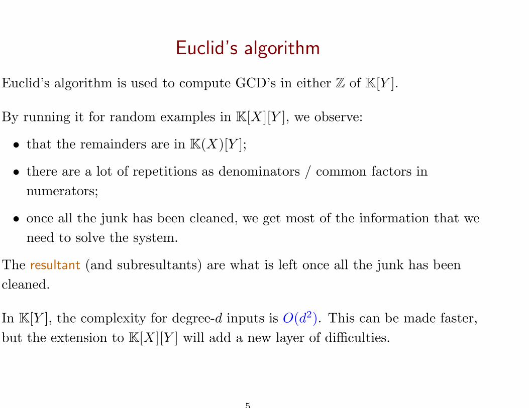
Euclid’s algorithm is used to compute GCD’s in either Z of K[Y ].
By running it for random examples in K[X ][Y ], we observe:
• that the remainders are in K(X)[Y ];
• there are a lot of repetitions as denominators / common factors in
numerators;
• once all the junk has been cleaned, we get most of the information that we
need to solve the system.
The resultant (and subresultants) are what is left once all the junk has been
cleaned.
4
Euclid’s algorithm
Euclid’s algorithm is used to compute GCD’s in either Z of K[Y ].
By running it for random examples in K[X ][Y ], we observe:
• that the remainders are in K(X)[Y ];
• there are a lot of repetitions as denominators / common factors in
numerators;
• once all the junk has been cleaned, we get most of the information that we
need to solve the system.
The resultant (and subresultants) are what is left once all the junk has been
cleaned.
In K[Y ], the complexity for degree-d inputs is O(d2). This can be made faster,
but the extension to K[X ][Y ] will add a new layer of difficulties.
5
Intersection of plane curves
6
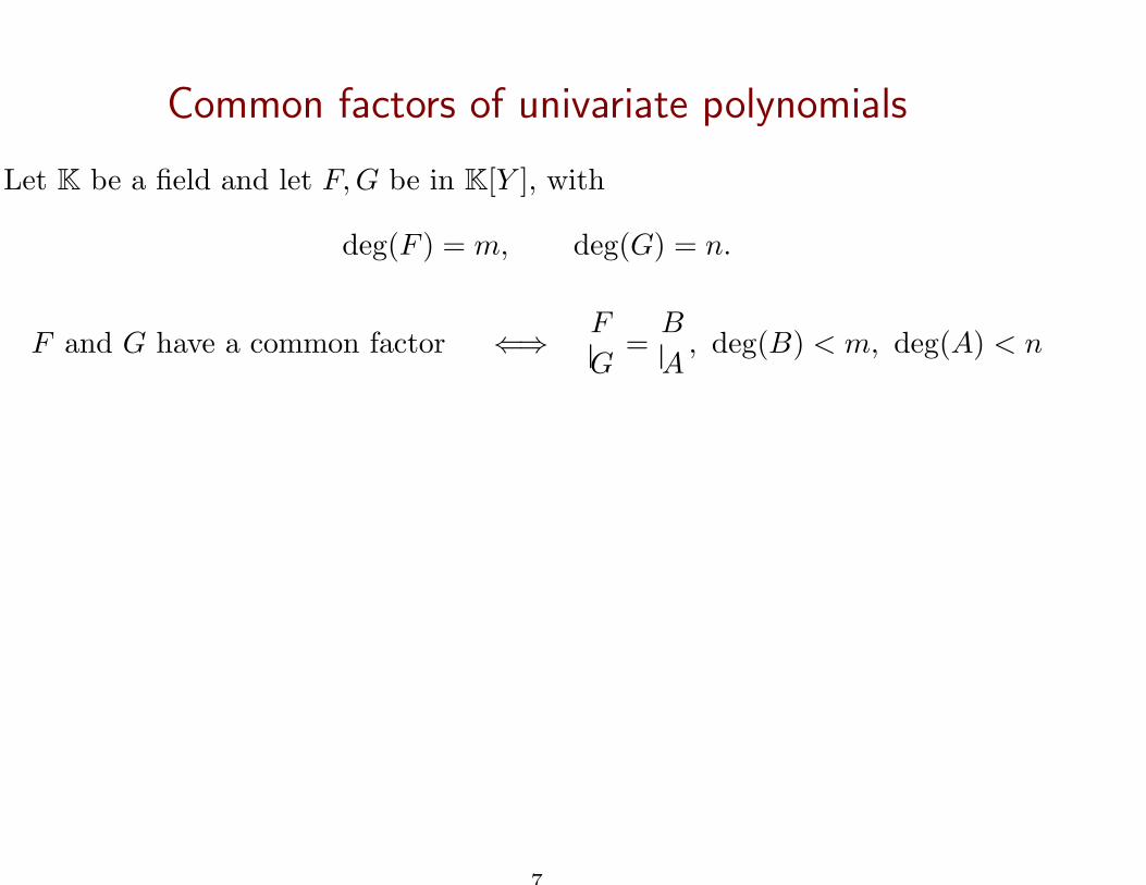
Common factors of univariate polynomials
Let K be a field and let F, G be in K[Y ], with
deg(F ) = m, deg(G) = n.
F and G have a common factor ⇐⇒F
G=
B
A, deg(B) < m, deg(A) < n
7
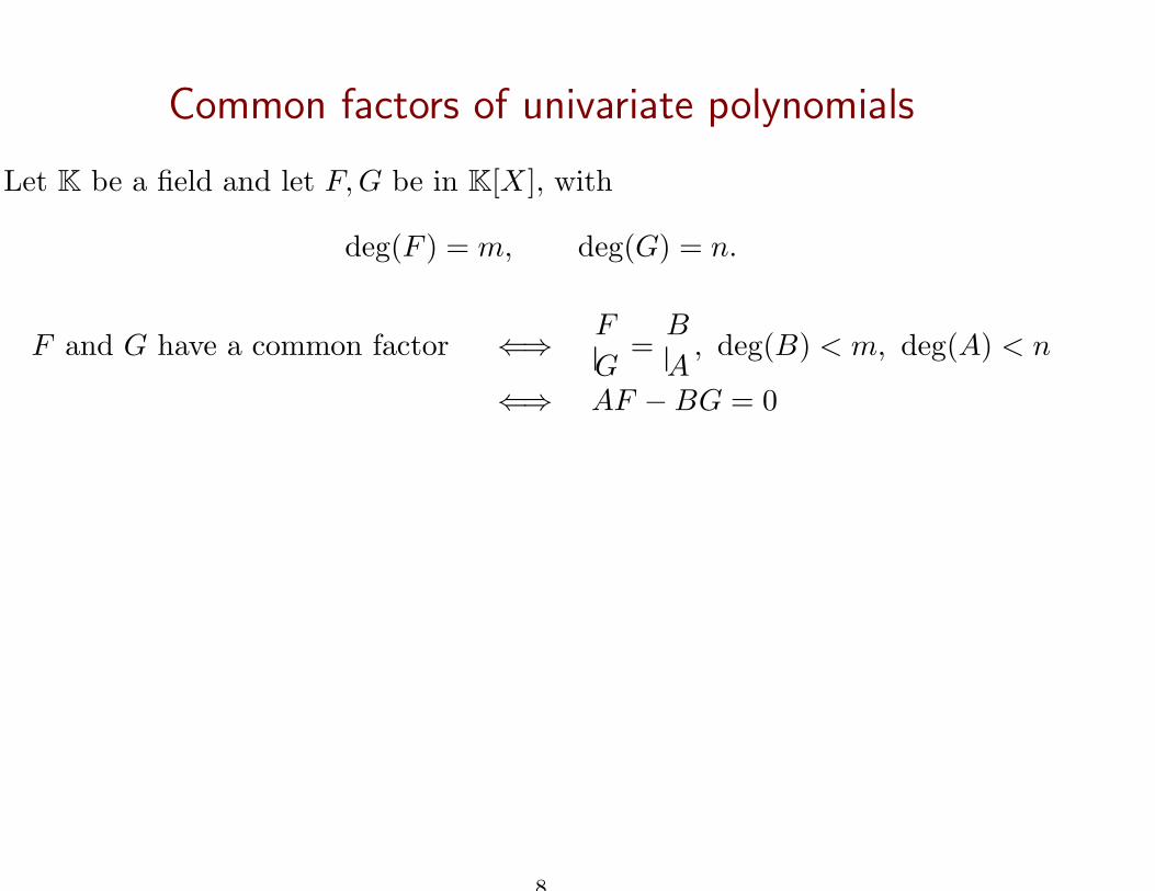
Common factors of univariate polynomials
Let K be a field and let F, G be in K[X ], with
deg(F ) = m, deg(G) = n.
F and G have a common factor ⇐⇒F
G=
B
A, deg(B) < m, deg(A) < n
⇐⇒ AF − BG = 0
8
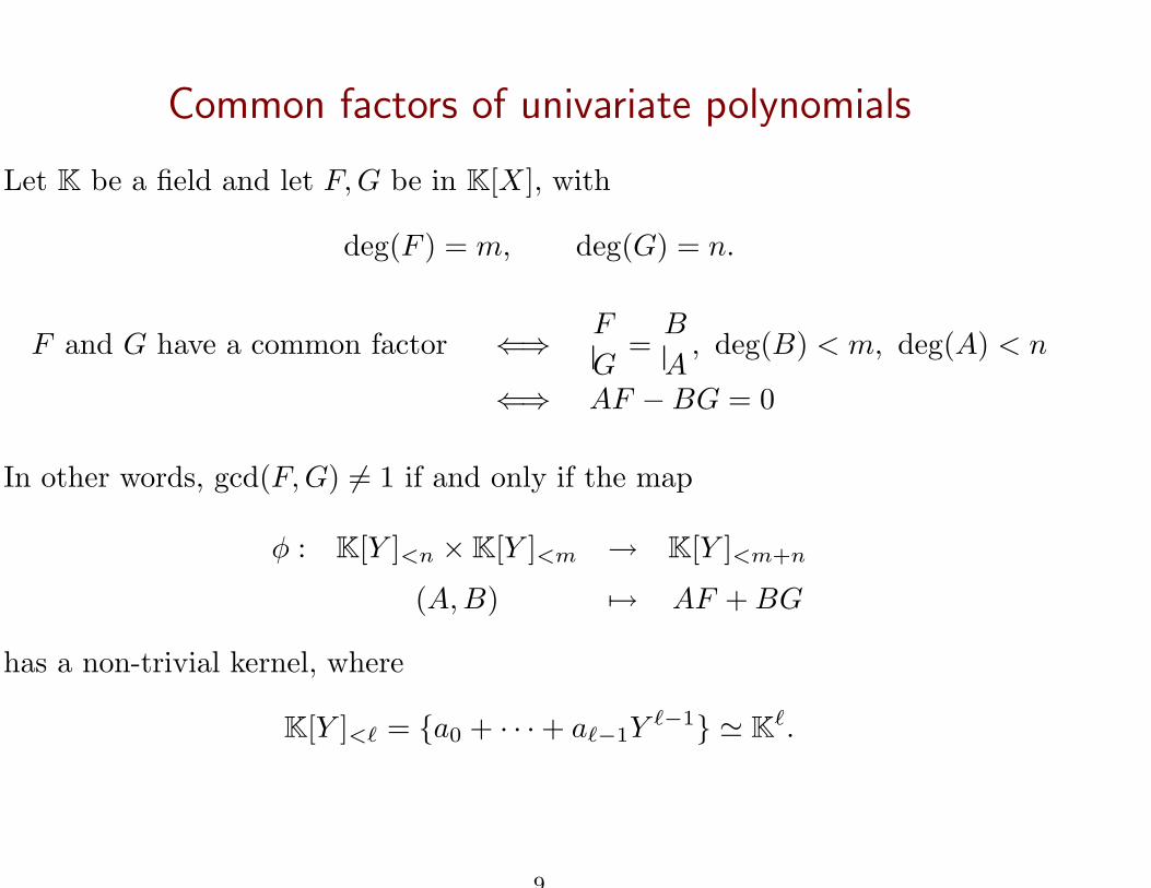
Common factors of univariate polynomials
Let K be a field and let F, G be in K[X ], with
deg(F ) = m, deg(G) = n.
F and G have a common factor ⇐⇒F
G=
B
A, deg(B) < m, deg(A) < n
⇐⇒ AF − BG = 0
In other words, gcd(F, G) 6= 1 if and only if the map
φ : K[Y ]<n × K[Y ]<m → K[Y ]<m+n
(A, B) 7→ AF + BG
has a non-trivial kernel, where
K[Y ]<ℓ = {a0 + · · · + aℓ−1Yℓ−1} ≃ Kℓ.
9
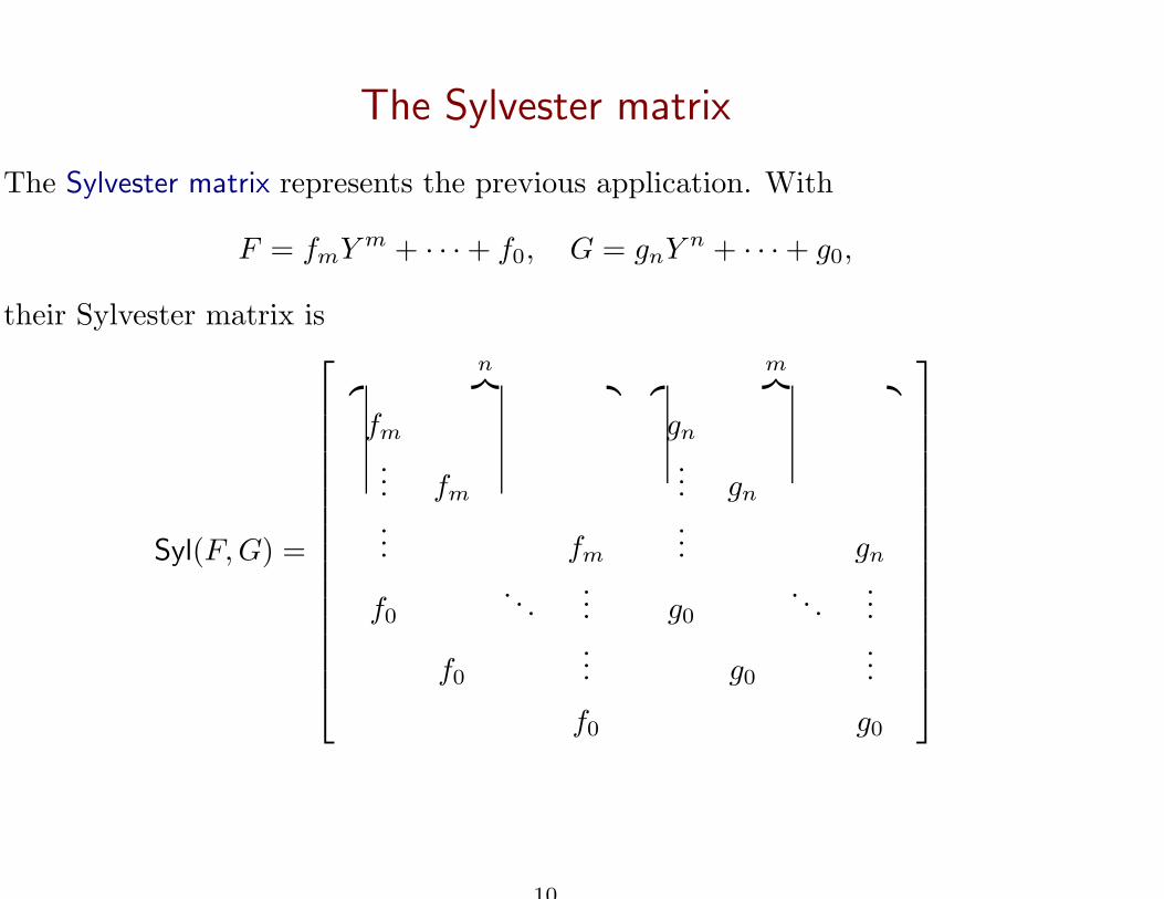
The Sylvester matrix
The Sylvester matrix represents the previous application. With
F = fmY m + · · · + f0, G = gnY n + · · · + g0,
their Sylvester matrix is
Syl(F, G) =
n︷ ︸︸ ︷
fm
... fm
... fm
f0. . .
...
f0
...
f0
m︷ ︸︸ ︷
gn
... gn
... gn
g0. . .
...
g0
...
g0
10
Resultant
Definition The resultant res(F, G) of F, G ∈ K[Y ] is the determinant of their
Sylvester matrix.
11
Resultant
Definition The resultant res(F, G) of F, G ∈ K[Y ] is the determinant of their
Sylvester matrix.
Proposition res(F, G) = 0 ⇐⇒ gcd(F, G) 6= 1.
12
Resultant
Definition The resultant res(F, G) of F, G ∈ K[Y ] is the determinant of their
Sylvester matrix.
Proposition res(F, G) = 0 ⇐⇒ gcd(F, G) 6= 1.
We extend the definition to polynomials F, G with coefficients in a ring R.
(warning: GCD’s do not really make sense over a general ring).
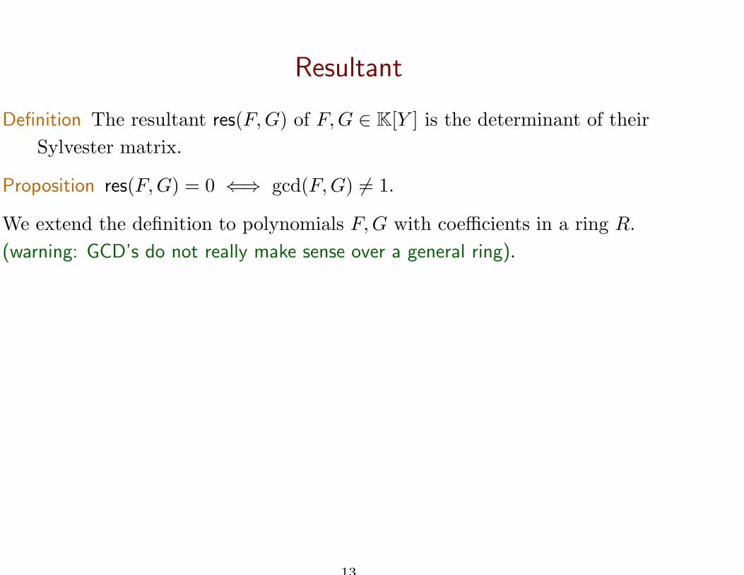
13
Resultant
Definition The resultant res(F, G) of F, G ∈ K[Y ] is the determinant of their
Sylvester matrix.
Proposition res(F, G) = 0 ⇐⇒ gcd(F, G) 6= 1.
We extend the definition to polynomials F, G with coefficients in a ring R.
(warning: GCD’s do not really make sense over a general ring).
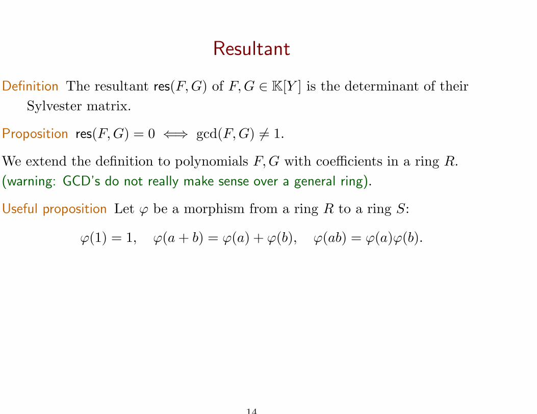
Useful proposition Let ϕ be a morphism from a ring R to a ring S:
ϕ(1) = 1, ϕ(a + b) = ϕ(a) + ϕ(b), ϕ(ab) = ϕ(a)ϕ(b).
14
Resultant
Definition The resultant res(F, G) of F, G ∈ K[Y ] is the determinant of their
Sylvester matrix.
Proposition res(F, G) = 0 ⇐⇒ gcd(F, G) 6= 1.
We extend the definition to polynomials F, G with coefficients in a ring R.
(warning: GCD’s do not really make sense over a general ring).
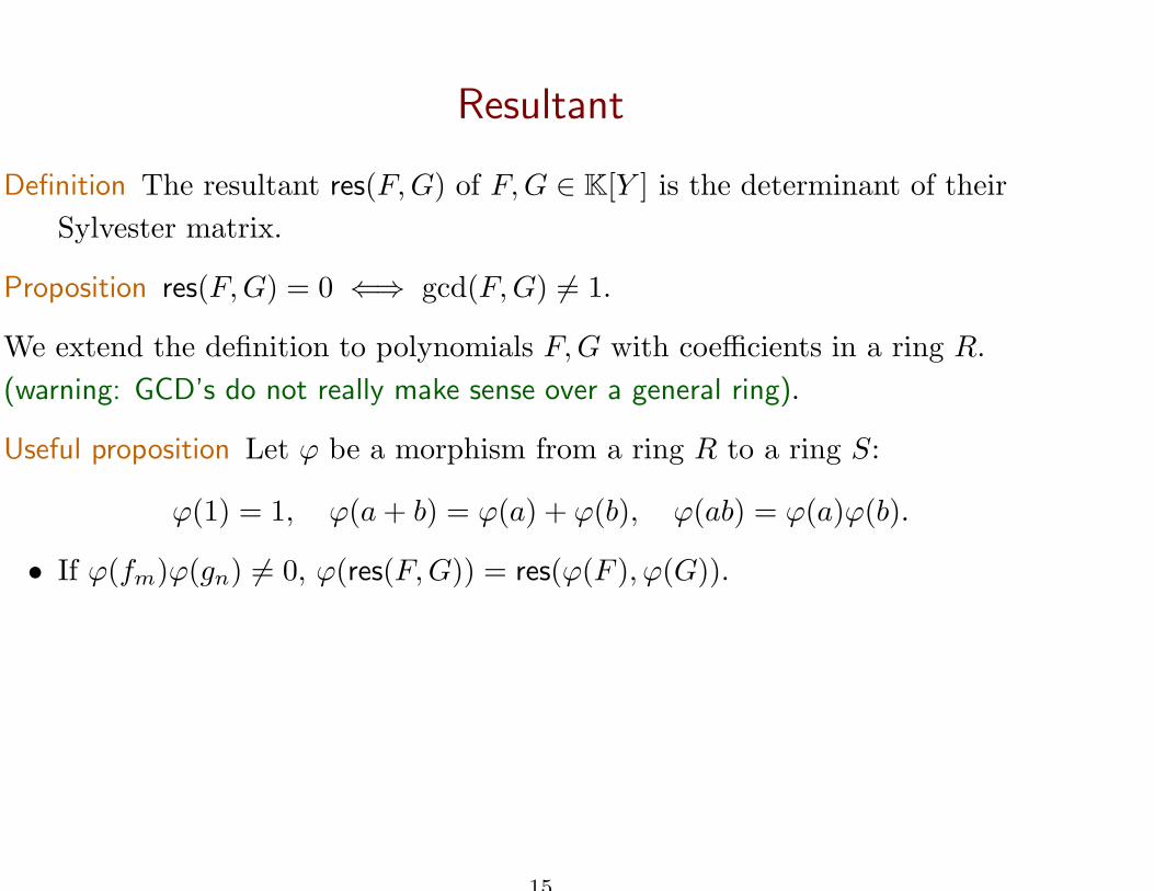
Useful proposition Let ϕ be a morphism from a ring R to a ring S:
ϕ(1) = 1, ϕ(a + b) = ϕ(a) + ϕ(b), ϕ(ab) = ϕ(a)ϕ(b).
• If ϕ(fm)ϕ(gn) 6= 0, ϕ(res(F, G)) = res(ϕ(F ), ϕ(G)).
15
Resultant
Definition The resultant res(F, G) of F, G ∈ K[Y ] is the determinant of their
Sylvester matrix.
Proposition res(F, G) = 0 ⇐⇒ gcd(F, G) 6= 1.
We extend the definition to polynomials F, G with coefficients in a ring R.
(warning: GCD’s do not really make sense over a general ring).
Useful proposition Let ϕ be a morphism from a ring R to a ring S:
ϕ(1) = 1, ϕ(a + b) = ϕ(a) + ϕ(b), ϕ(ab) = ϕ(a)ϕ(b).
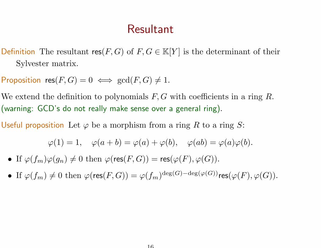
• If ϕ(fm)ϕ(gn) 6= 0 then ϕ(res(F, G)) = res(ϕ(F ), ϕ(G)).
• If ϕ(fm) 6= 0 then ϕ(res(F, G)) = ϕ(fm)deg(G)−deg(ϕ(G))res(ϕ(F ), ϕ(G)).
16
Resultant
Definition The resultant res(F, G) of F, G ∈ K[Y ] is the determinant of their
Sylvester matrix.
Proposition res(F, G) = 0 ⇐⇒ gcd(F, G) 6= 1.
We extend the definition to polynomials F, G with coefficients in a ring R.
(warning: GCD’s do not really make sense over a general ring).
Useful proposition Let ϕ be a morphism from a ring R to a ring S:
ϕ(1) = 1, ϕ(a + b) = ϕ(a) + ϕ(b), ϕ(ab) = ϕ(a)ϕ(b).
• If ϕ(fm)ϕ(gn) 6= 0 then ϕ(res(F, G)) = res(ϕ(F ), ϕ(G)).
• If ϕ(fm) 6= 0 then ϕ(res(F, G)) = ϕ(fm)deg(G)−deg(ϕ(G))res(ϕ(F ), ϕ(G)).
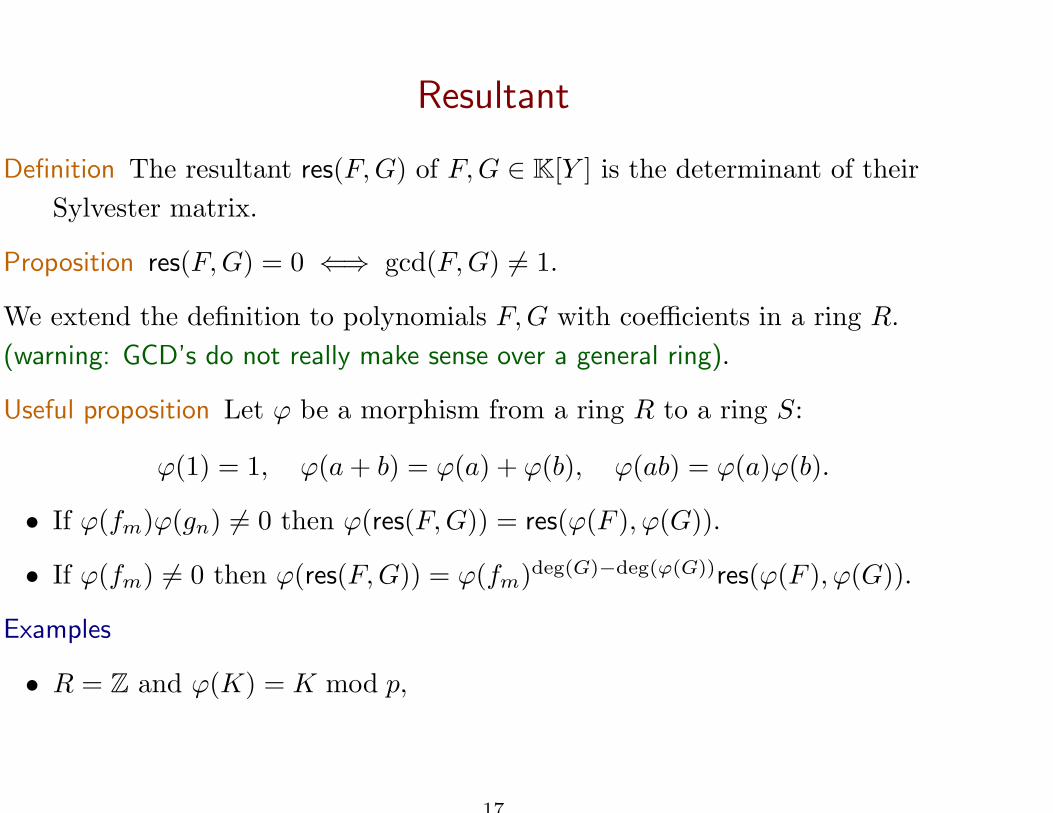
Examples
• R = Z and ϕ(K) = K mod p,
17
Resultant
Definition The resultant res(F, G) of F, G ∈ K[Y ] is the determinant of their
Sylvester matrix.
Proposition res(F, G) = 0 ⇐⇒ gcd(F, G) 6= 1.
We extend the definition to polynomials F, G with coefficients in a ring R.
(warning: GCD’s do not really make sense over a general ring).
Useful proposition Let ϕ be a morphism from a ring R to a ring S:
ϕ(1) = 1, ϕ(a + b) = ϕ(a) + ϕ(b), ϕ(ab) = ϕ(a)ϕ(b).
• If ϕ(fm)ϕ(gn) 6= 0 then ϕ(res(F, G)) = res(ϕ(F ), ϕ(G)).
• If ϕ(fm) 6= 0 then ϕ(res(F, G)) = ϕ(fm)deg(G)−deg(ϕ(G))res(ϕ(F ), ϕ(G)).
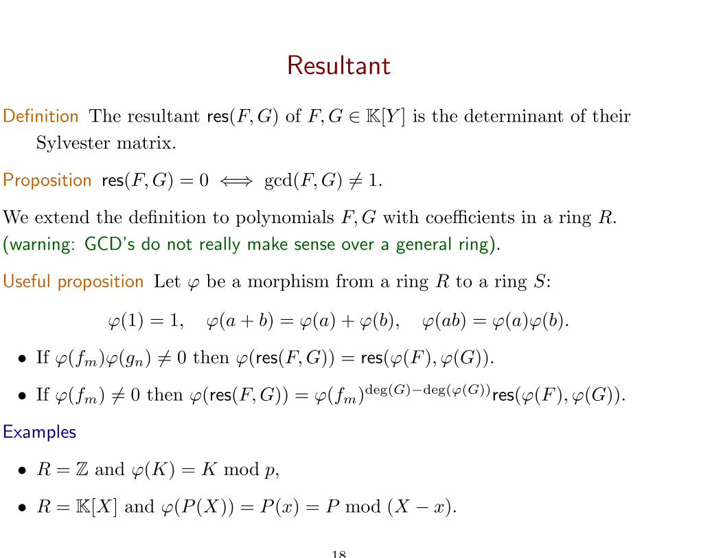
Examples
• R = Z and ϕ(K) = K mod p,
• R = K[X ] and ϕ(P (X)) = P (x) = P mod (X − x).
18
Application to the intersection of curves
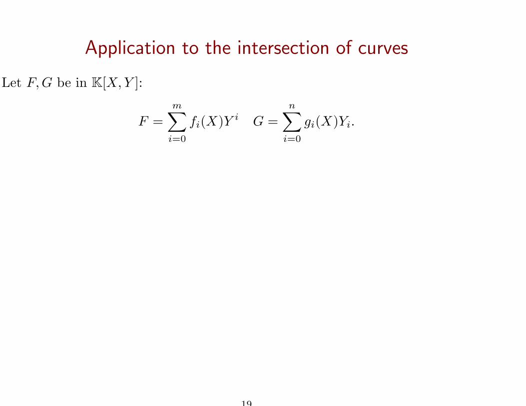
Let F, G be in K[X, Y ]:
F =m∑
i=0
fi(X)Y i G =n∑
i=0
gi(X)Yi.
19
Application to the intersection of curves
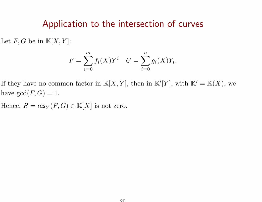
Let F, G be in K[X, Y ]:
F =m∑
i=0
fi(X)Y i G =n∑
i=0
gi(X)Yi.
If they have no common factor in K[X, Y ], then in K′[Y ], with K′ = K(X), we
have gcd(F, G) = 1.
Hence, R = resY (F, G) ∈ K[X ] is not zero.
20
Application to the intersection of curves
Let F, G be in K[X, Y ]:
F =m∑
i=0
fi(X)Y i G =n∑
i=0
gi(X)Yi.
If they have no common factor in K[X, Y ], then in K′[Y ], with K′ = K(X), we
have gcd(F, G) = 1.
Hence, R = resY (F, G) ∈ K[X ] is not zero.
Proposition. Let x be in K. Then R(x) = 0 if and only if
• fm(x) = gn(x) = 0
• or there exists y such that F (x, y) = G(x, y) = 0.
21
Application to the intersection of curves
Let F, G be in K[X, Y ]:
F =m∑
i=0
fi(X)Y i G =n∑
i=0
gi(X)Yi.
If they have no common factor in K[X, Y ], then in K′[Y ], with K′ = K(X), we
have gcd(F, G) = 1.
Hence, R = resY (F, G) ∈ K[X ] is not zero.
Proposition. Let x be in K. Then R(x) = 0 if and only if
• fm(x) = gn(x) = 0
• or there exists y such that F (x, y) = G(x, y) = 0.
Proof. If fm(x) = gn(x) = 0, R(x) = 0.
Suppose now that e.g. fm(x) 6= 0.
Then R(x) = fm(x)k res(F (x, Y ), G(x, Y )), so R(x) = 0 if and only if
F (x, Y ) and G(x, Y ) have a common factor.
22
A degenerate example
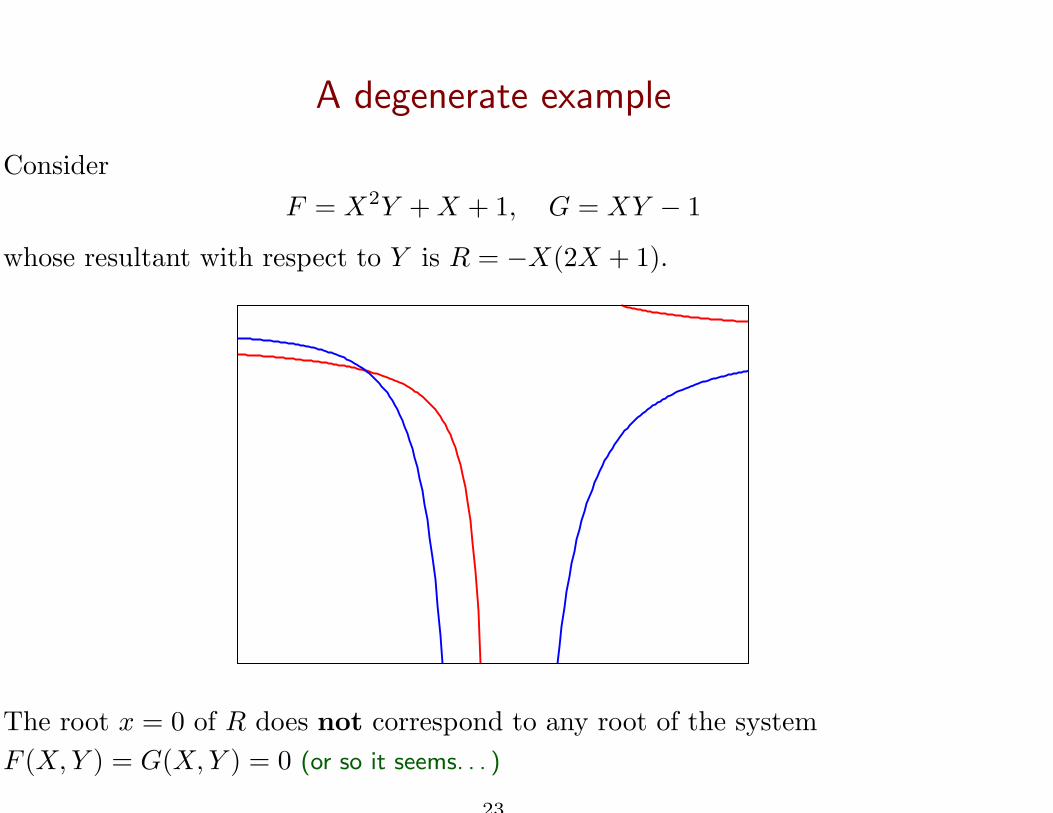
Consider
F = X2Y + X + 1, G = XY − 1
whose resultant with respect to Y is R = −X(2X + 1).
The root x = 0 of R does not correspond to any root of the system
F (X, Y ) = G(X, Y ) = 0 (or so it seems. . . )
23
Curves in generic position
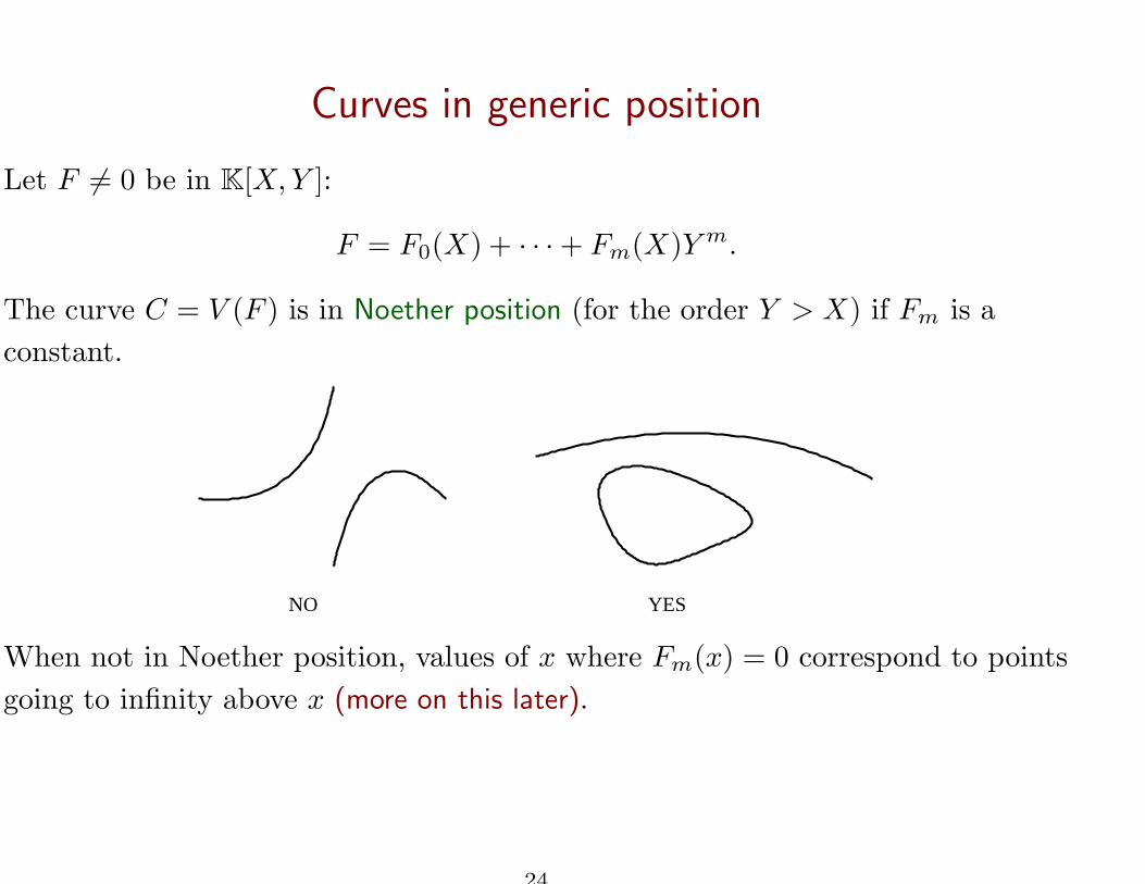
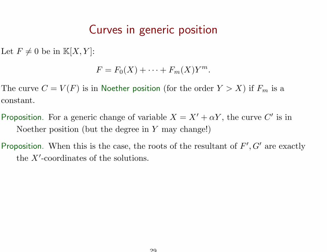
Let F 6= 0 be in K[X, Y ]:
F = F0(X) + · · · + Fm(X)Y m.
The curve C = V (F ) is in Noether position (for the order Y > X) if Fm is a
constant.
NO YES
When not in Noether position, values of x where Fm(x) = 0 correspond to points
going to infinity above x (more on this later).
24
Curves in generic position
Let F 6= 0 be in K[X, Y ]:
F = F0(X) + · · · + Fm(X)Y m.
The curve C = V (F ) is in Noether position (for the order Y > X) if Fm is a
constant.
Proposition. For a generic change of variable X = X ′ + αY , the curve C ′ is in
Noether position (but the degree in Y may change!)
25
Curves in generic position
Let F 6= 0 be in K[X, Y ]:
F = F0(X) + · · · + Fm(X)Y m.
The curve C = V (F ) is in Noether position (for the order Y > X) if Fm is a
constant.
Proposition. For a generic change of variable X = X ′ + αY , the curve C ′ is in
Noether position (but the degree in Y may change!)
Proof. Let d be the total degree of F and let H be the homogeneous part of degree
d of F . Write H =∑
hiXiY d−i.
26
Curves in generic position
Let F 6= 0 be in K[X, Y ]:
F = F0(X) + · · · + Fm(X)Y m.
The curve C = V (F ) is in Noether position (for the order Y > X) if Fm is a
constant.
Proposition. For a generic change of variable X = X ′ + αY , the curve C ′ is in
Noether position (but the degree in Y may change!)
Proof. Let d be the total degree of F and let H be the homogeneous part of degree
d of F . Write H =∑
hiXiY d−i.
Then
H(X ′ + αY, Y ) =∑
hi(X′ + αY )iY d−i = Y d
∑
hiαi + · · ·
27
Curves in generic position
Let F 6= 0 be in K[X, Y ]:
F = F0(X) + · · · + Fm(X)Y m.
The curve C = V (F ) is in Noether position (for the order Y > X) if Fm is a
constant.
Proposition. For a generic change of variable X = X ′ + αY , the curve C ′ is in
Noether position (but the degree in Y may change!)
Proof. Let d be the total degree of F and let H be the homogeneous part of degree
d of F . Write H =∑
hiXiY d−i.
Then
H(X ′ + αY, Y ) =∑
hi(X′ + αY )iY d−i = Y d
∑
hiαi + · · ·
So it suffices that α is not a root of∑
hiAi.
28
Curves in generic position
Let F 6= 0 be in K[X, Y ]:
F = F0(X) + · · · + Fm(X)Y m.
The curve C = V (F ) is in Noether position (for the order Y > X) if Fm is a
constant.
Proposition. For a generic change of variable X = X ′ + αY , the curve C ′ is in
Noether position (but the degree in Y may change!)
Proposition. When this is the case, the roots of the resultant of F ′, G′ are exactly
the X ′-coordinates of the solutions.
29
Finiteness of the solution set
Proposition. Let F, G be in K[X, Y ] with a common factor. Then V (F, G) is
finite.
30
Finiteness of the solution set
Proposition. Let F, G be in K[X, Y ] with a common factor. Then V (F, G) is
finite.
Proof. Suppose that the curves C = V (F ) and C ′ = V (G) are both in Noether
position.
31
Finiteness of the solution set
Proposition. Let F, G be in K[X, Y ] with a common factor. Then V (F, G) is
finite.
Proof. Suppose that the curves C = V (F ) and C ′ = V (G) are both in Noether
position.
Let R ∈ K[X ] be the resultant of F and G with respect to Y , so that R 6= 0.
Each solution of F (x, y) = G(x, y) = 0 satisfies R(x) = 0.
32
Finiteness of the solution set
Proposition. Let F, G be in K[X, Y ] with a common factor. Then V (F, G) is
finite.
Proof. Suppose that the curves C = V (F ) and C ′ = V (G) are both in Noether
position.
Let R ∈ K[X ] be the resultant of F and G with respect to Y , so that R 6= 0.
Each solution of F (x, y) = G(x, y) = 0 satisfies R(x) = 0.
• R has a finite number of roots.
33
Finiteness of the solution set
Proposition. Let F, G be in K[X, Y ] with a common factor. Then V (F, G) is
finite.
Proof. Suppose that the curves C = V (F ) and C ′ = V (G) are both in Noether
position.
Let R ∈ K[X ] be the resultant of F and G with respect to Y , so that R 6= 0.
Each solution of F (x, y) = G(x, y) = 0 satisfies R(x) = 0.
• R has a finite number of roots.
• For any root x of R, there is a finite number of y such that F (x, y) = 0.
34
Curves in generic position, continued
Proposition. Let F, G be in K[X, Y ] with a common factor, of total degrees at
most d.
For a generic choice of X ′ = X − αY , X ′ is a separating element for
V = V (F, G).
35
Curves in generic position, continued
Proposition. Let F, G be in K[X, Y ] with a common factor, of total degrees at
most d.
For a generic choice of X ′ = X − αY , X ′ is a separating element for
V = V (F, G).
Proof. Let {(xi, yi)}i≤N be the finite set of common solutions.
36
Curves in generic position, continued
Proposition. Let F, G be in K[X, Y ] with a common factor, of total degrees at
most d.
For a generic choice of X ′ = X − αY , X ′ is a separating element for
V = V (F, G).
Proof. Let {(xi, yi)}i≤N be the finite set of common solutions.
Through the change of variables X ′ = X − αY , the solution set becomes
{xi − αyi, yi}i≤N .
37
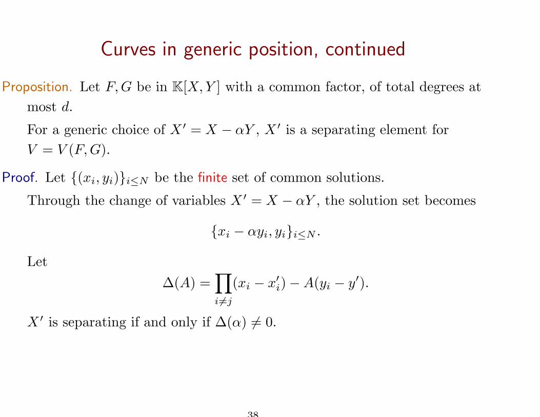
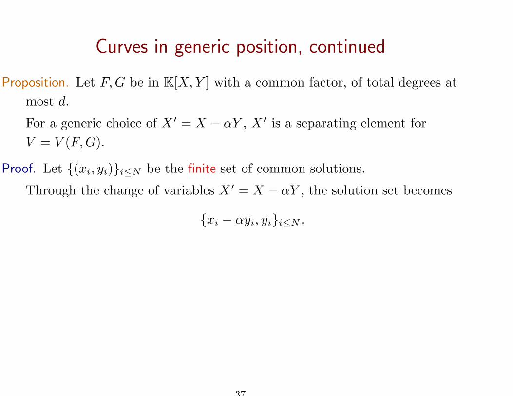
Curves in generic position, continued
Proposition. Let F, G be in K[X, Y ] with a common factor, of total degrees at
most d.
For a generic choice of X ′ = X − αY , X ′ is a separating element for
V = V (F, G).
Proof. Let {(xi, yi)}i≤N be the finite set of common solutions.
Through the change of variables X ′ = X − αY , the solution set becomes
{xi − αyi, yi}i≤N .
Let
∆(A) =∏
i 6=j
(xi − x′i) − A(yi − y′).
X ′ is separating if and only if ∆(α) 6= 0.
38
Cardinality of the intersection
Proposition. Let F, G be in K[X, Y ] with a common factor, of total degrees at
most d. Then V (F, G) has cardinality at most d2.
39
Cardinality of the intersection
Proposition. Let F, G be in K[X, Y ] with a common factor, of total degrees at
most d. Then V (F, G) has cardinality at most d2.
Proof. By a generic change of variables, we can suppose that X is a separating
element for V = V (F, G) and that the curves are in Noether position.
40
Cardinality of the intersection
Proposition. Let F, G be in K[X, Y ] with a common factor, of total degrees at
most d. Then V (F, G) has cardinality at most d2.
Proof. By a generic change of variables, we can suppose that X is a separating
element for V = V (F, G) and that the curves are in Noether position.
This does not change the total degree, or the number of solutions!
41
Cardinality of the intersection
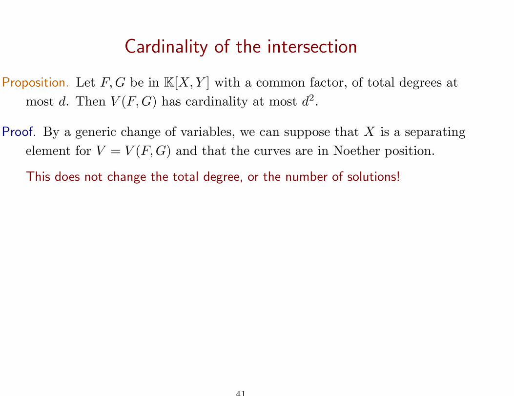
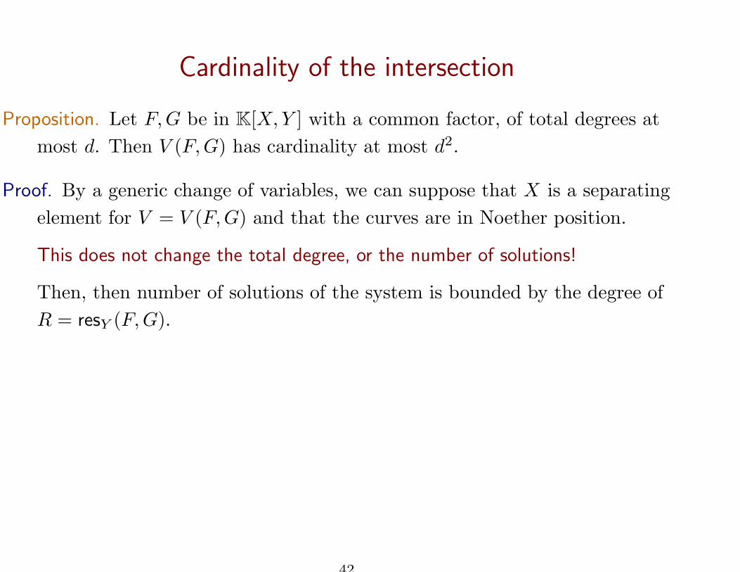
Proposition. Let F, G be in K[X, Y ] with a common factor, of total degrees at
most d. Then V (F, G) has cardinality at most d2.
Proof. By a generic change of variables, we can suppose that X is a separating
element for V = V (F, G) and that the curves are in Noether position.
This does not change the total degree, or the number of solutions!
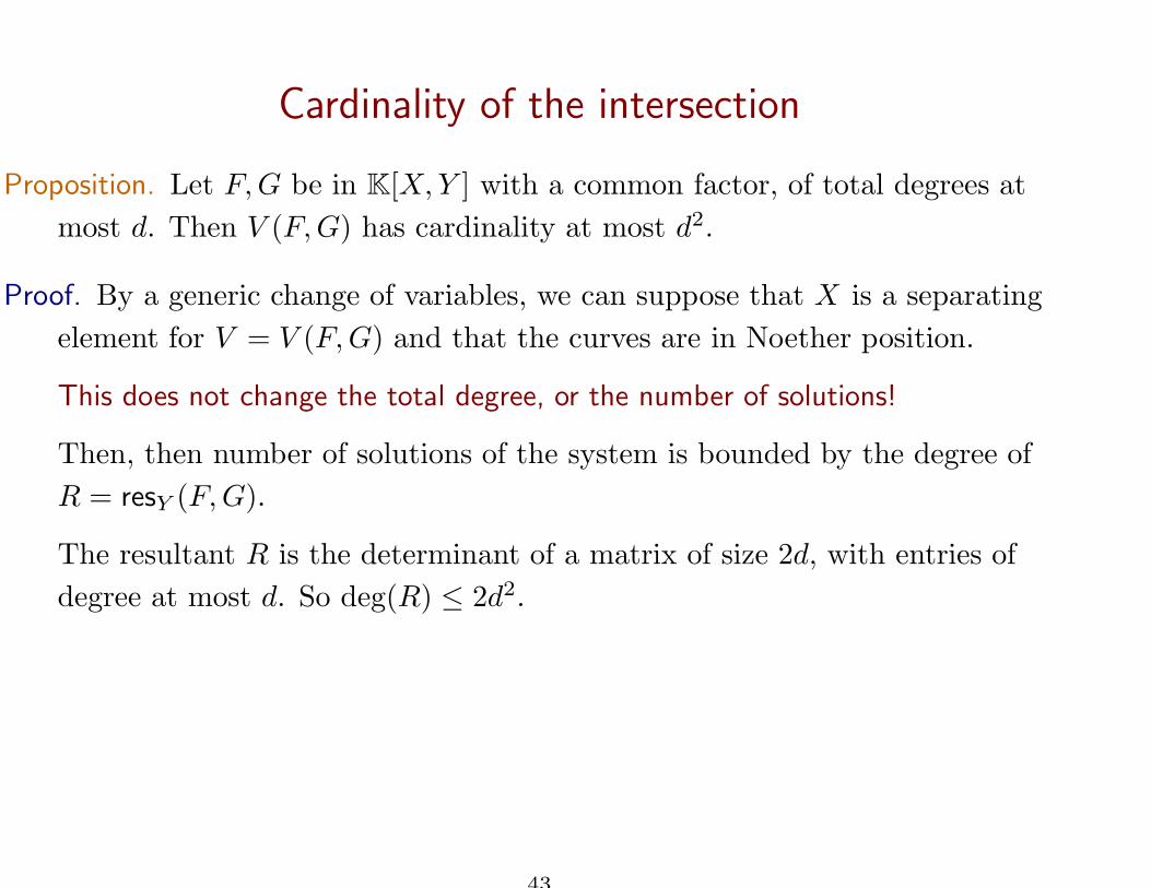
Then, then number of solutions of the system is bounded by the degree of
R = resY (F, G).
42
Cardinality of the intersection
Proposition. Let F, G be in K[X, Y ] with a common factor, of total degrees at
most d. Then V (F, G) has cardinality at most d2.
Proof. By a generic change of variables, we can suppose that X is a separating
element for V = V (F, G) and that the curves are in Noether position.
This does not change the total degree, or the number of solutions!
Then, then number of solutions of the system is bounded by the degree of
R = resY (F, G).
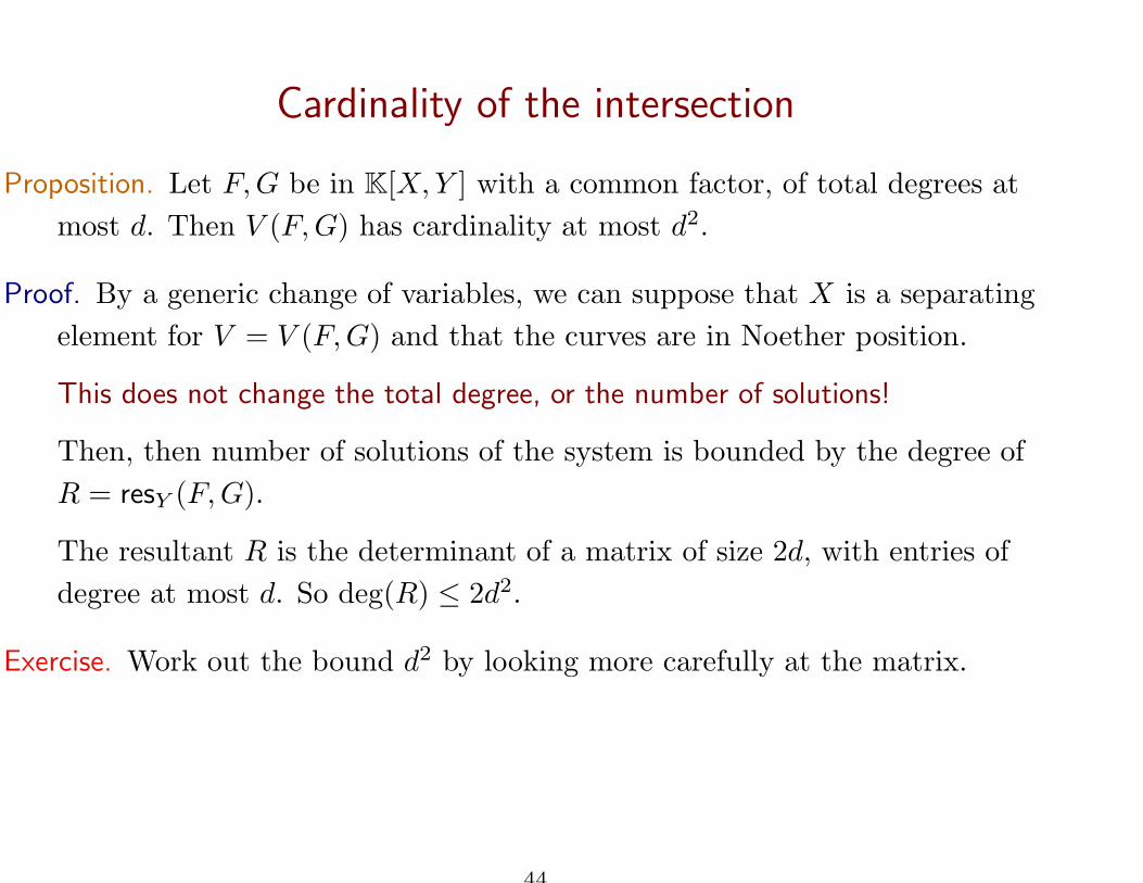
The resultant R is the determinant of a matrix of size 2d, with entries of
degree at most d. So deg(R) ≤ 2d2.
43
Cardinality of the intersection
Proposition. Let F, G be in K[X, Y ] with a common factor, of total degrees at
most d. Then V (F, G) has cardinality at most d2.
Proof. By a generic change of variables, we can suppose that X is a separating
element for V = V (F, G) and that the curves are in Noether position.
This does not change the total degree, or the number of solutions!
Then, then number of solutions of the system is bounded by the degree of
R = resY (F, G).
The resultant R is the determinant of a matrix of size 2d, with entries of
degree at most d. So deg(R) ≤ 2d2.
Exercise. Work out the bound d2 by looking more carefully at the matrix.
44
Some properties of the resultant
45
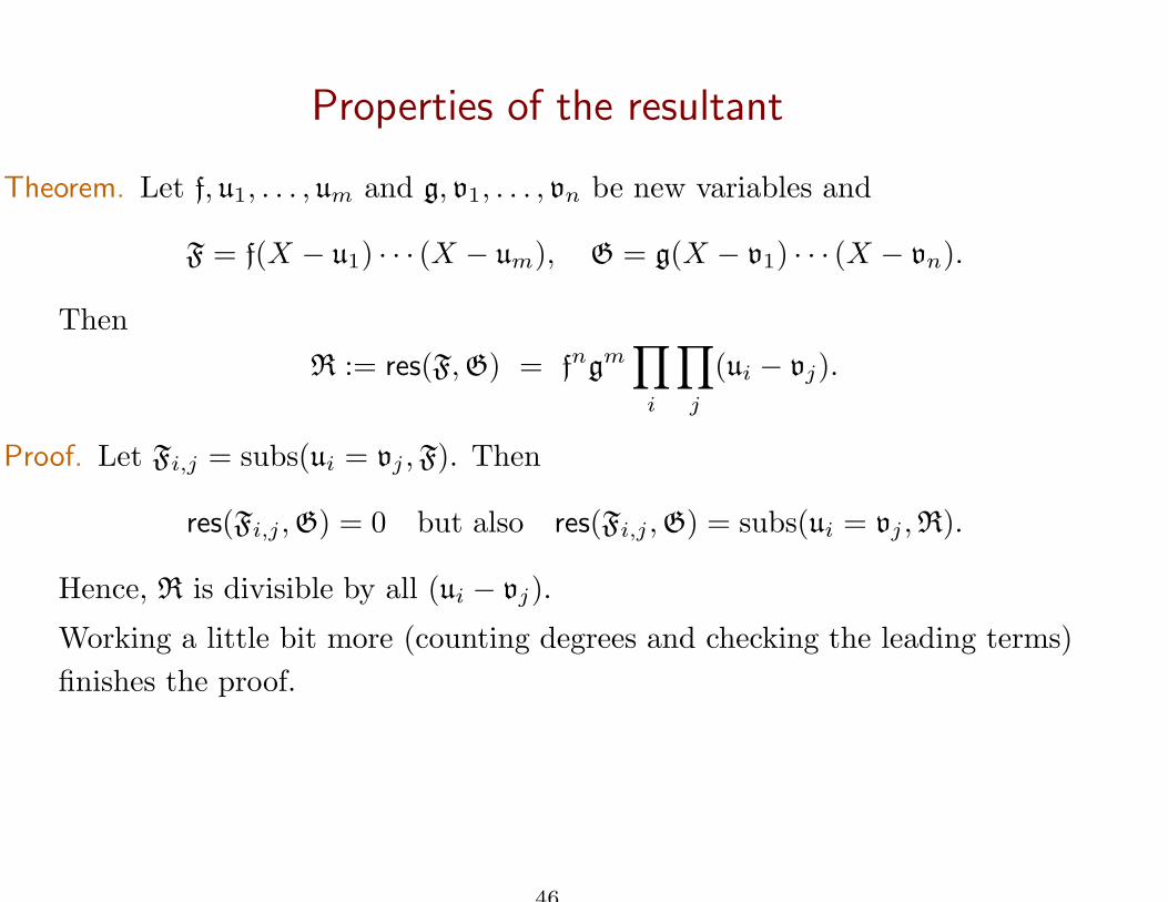
Properties of the resultant
Theorem. Let f, u1, . . . , um and g, v1, . . . , vn be new variables and
F = f(X − u1) · · · (X − um), G = g(X − v1) · · · (X − vn).
Then
R := res(F, G) = fngm∏
i
∏
j
(ui − vj).
Proof. Let Fi,j = subs(ui = vj , F). Then
res(Fi,j , G) = 0 but also res(Fi,j , G) = subs(ui = vj , R).
Hence, R is divisible by all (ui − vj).
Working a little bit more (counting degrees and checking the leading terms)
finishes the proof.
46
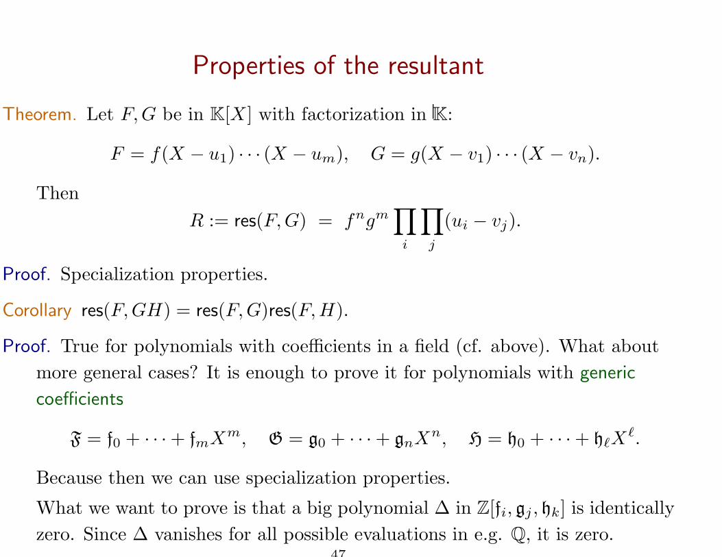
Properties of the resultant
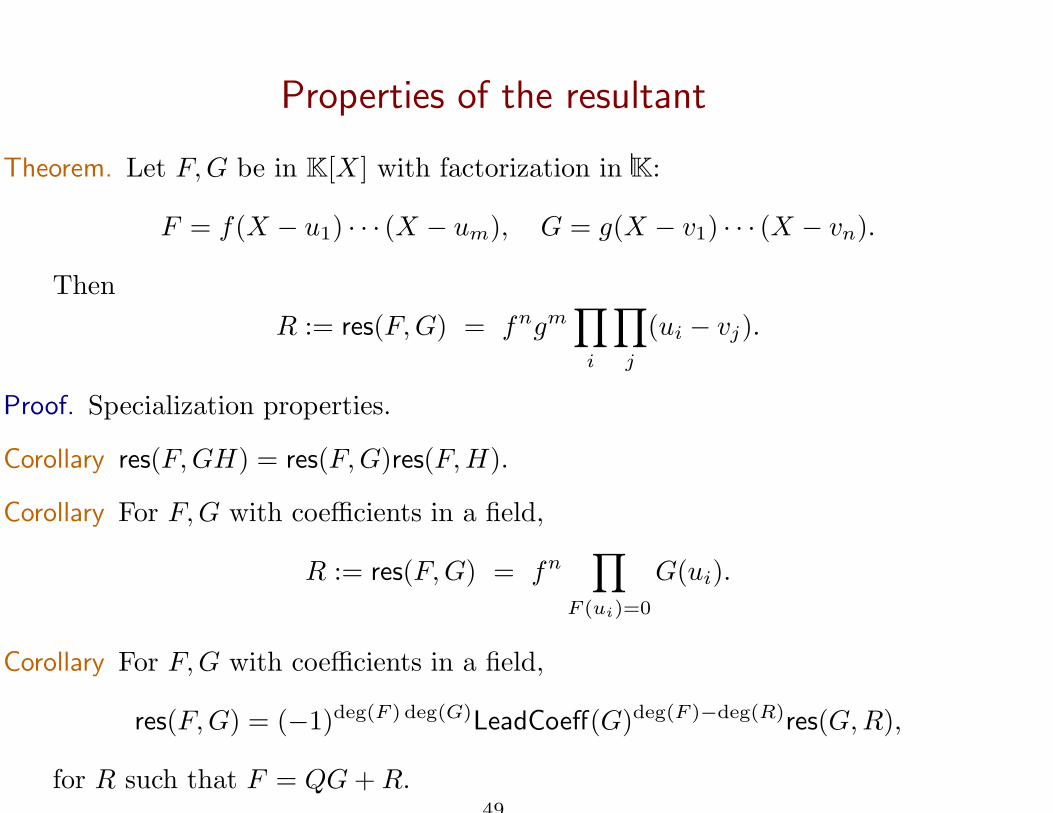
Theorem. Let F, G be in K[X ] with factorization in K:
F = f(X − u1) · · · (X − um), G = g(X − v1) · · · (X − vn).
Then
R := res(F, G) = fngm∏
i
∏
j
(ui − vj).
Proof. Specialization properties.
Corollary res(F, GH) = res(F, G)res(F, H).
Proof. True for polynomials with coefficients in a field (cf. above). What about
more general cases? It is enough to prove it for polynomials with generic
coefficients
F = f0 + · · · + fmXm, G = g0 + · · · + gnXn, H = h0 + · · · + hℓXℓ.
Because then we can use specialization properties.
What we want to prove is that a big polynomial ∆ in Z[fi, gj , hk] is identically
zero. Since ∆ vanishes for all possible evaluations in e.g. Q, it is zero.47
Properties of the resultant
Theorem. Let F, G be in K[X ] with factorization in K:
F = f(X − u1) · · · (X − um), G = g(X − v1) · · · (X − vn).
Then
R := res(F, G) = fngm∏
i
∏
j
(ui − vj).
Proof. Specialization properties.
Corollary res(F, GH) = res(F, G)res(F, H).
Corollary For F, G with coefficients in a field,
R := res(F, G) = fn∏
F (ui)=0
G(ui).
48
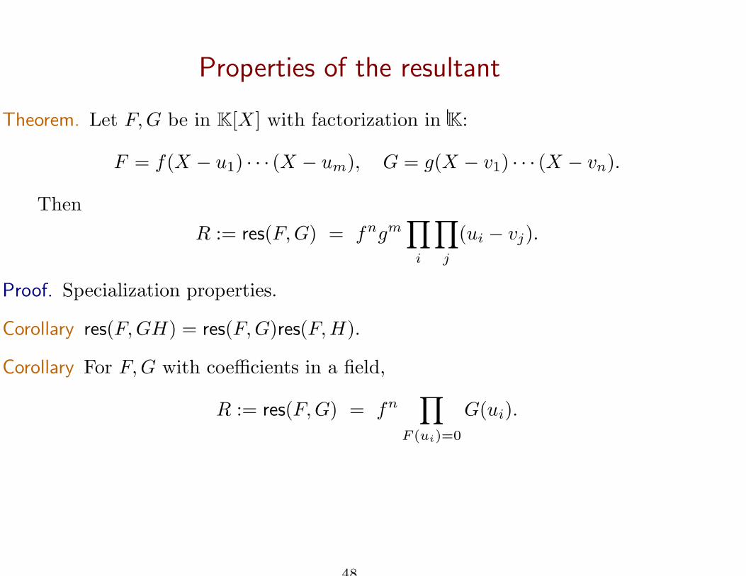
Properties of the resultant
Theorem. Let F, G be in K[X ] with factorization in K:
F = f(X − u1) · · · (X − um), G = g(X − v1) · · · (X − vn).
Then
R := res(F, G) = fngm∏
i
∏
j
(ui − vj).
Proof. Specialization properties.
Corollary res(F, GH) = res(F, G)res(F, H).
Corollary For F, G with coefficients in a field,
R := res(F, G) = fn∏
F (ui)=0
G(ui).
Corollary For F, G with coefficients in a field,
res(F, G) = (−1)deg(F ) deg(G)LeadCoeff(G)deg(F )−deg(R)res(G, R),
for R such that F = QG + R.49
Computing resultants
50
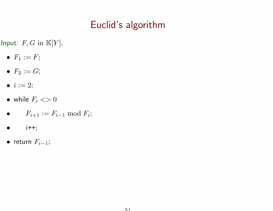
Euclid’s algorithm
Input: F, G in K[Y ].
• F1 := F ;
• F2 := G;
• i := 2;
• while Fi <> 0
• Fi+1 := Fi−1 mod Fi;
• i++;
• return Fi−1;
51
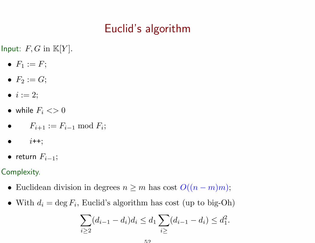
Euclid’s algorithm
Input: F, G in K[Y ].
• F1 := F ;
• F2 := G;
• i := 2;
• while Fi <> 0
• Fi+1 := Fi−1 mod Fi;
• i++;
• return Fi−1;
Complexity.
• Euclidean division in degrees n ≥ m has cost O((n − m)m);
• With di = deg Fi, Euclid’s algorithm has cost (up to big-Oh)∑
i≥2
(di−1 − di)di ≤ d1
∑
i≥
(di−1 − di) ≤ d21.
52
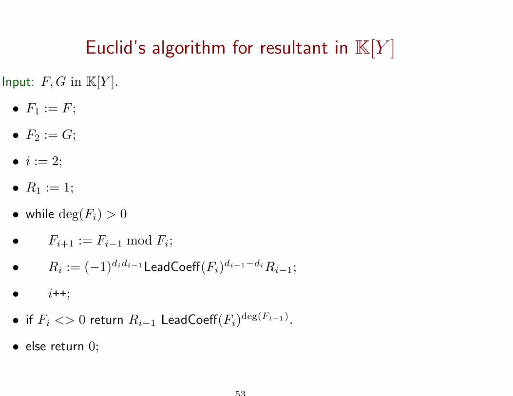
Euclid’s algorithm for resultant in K[Y ]
Input: F, G in K[Y ].
• F1 := F ;
• F2 := G;
• i := 2;
• R1 := 1;
• while deg(Fi) > 0
• Fi+1 := Fi−1 mod Fi;
• Ri := (−1)didi−1LeadCoeff(Fi)di−1−diRi−1;
• i++;
• if Fi <> 0 return Ri−1 LeadCoeff(Fi)deg(Fi−1).
• else return 0;
53
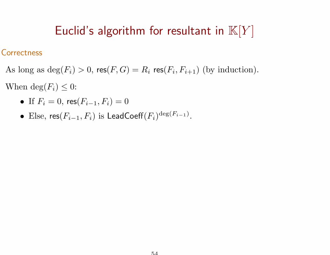
Euclid’s algorithm for resultant in K[Y ]
Correctness
As long as deg(Fi) > 0, res(F, G) = Ri res(Fi, Fi+1) (by induction).
When deg(Fi) ≤ 0:
• If Fi = 0, res(Fi−1, Fi) = 0
• Else, res(Fi−1, Fi) is LeadCoeff(Fi)deg(Fi−1).
54
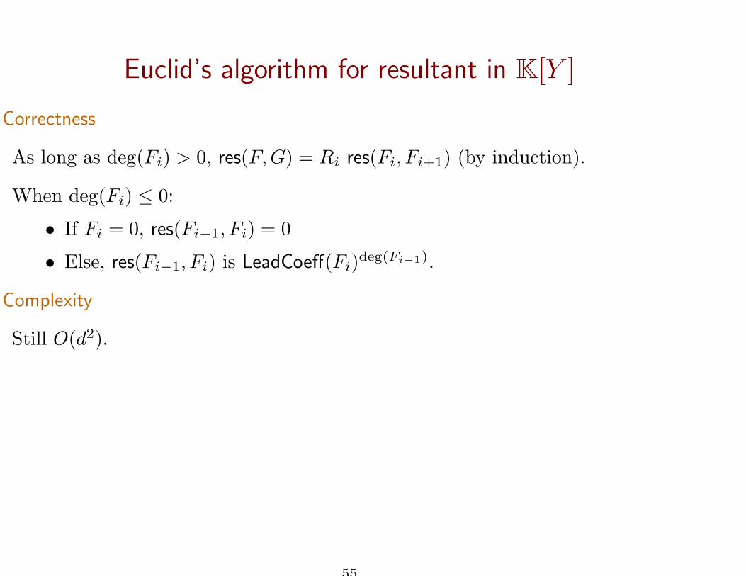
Euclid’s algorithm for resultant in K[Y ]
Correctness
As long as deg(Fi) > 0, res(F, G) = Ri res(Fi, Fi+1) (by induction).
When deg(Fi) ≤ 0:
• If Fi = 0, res(Fi−1, Fi) = 0
• Else, res(Fi−1, Fi) is LeadCoeff(Fi)deg(Fi−1).
Complexity
Still O(d2).
55
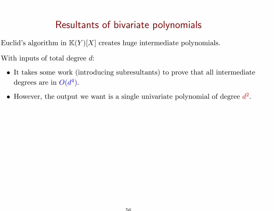
Resultants of bivariate polynomials
Euclid’s algorithm in K(Y )[X ] creates huge intermediate polynomials.
With inputs of total degree d:
• It takes some work (introducing subresultants) to prove that all intermediate
degrees are in O(d4).
• However, the output we want is a single univariate polynomial of degree d2.
56
Resultants of bivariate polynomials
Euclid’s algorithm in K(Y )[X ] creates huge intermediate polynomials.
With inputs of total degree d:
• It takes some work (introducing subresultants) to prove that all intermediate
degrees are in O(d4).
• However, the output we want is a single univariate polynomial of degree d2.
Two workarounds:
• Understand, predict and pre-clean the common factors and denominators;
• Use a modular algorithm.
57
Modular algorithm, plain version
Input: F, G in K[X, Y ] of total degrees ≤ d.
• Compute res(F (c, Y ), G(c, Y )) for d2 + 1 values of c (which do not cancel a
leading term);
• Interpolate the result.
58
Modular algorithm, plain version
Input: F, G in K[X, Y ] of total degrees ≤ d.
• Compute res(F (c, Y ), G(c, Y )) for d2 + 1 values of c (which do not cancel a
leading term);
• Interpolate the result.
Complexity.
• O(d2 × d2) + O(Costinterpolation(d2)) ∈ O(d4) (proof upcoming).
59
Interpolating polynomials
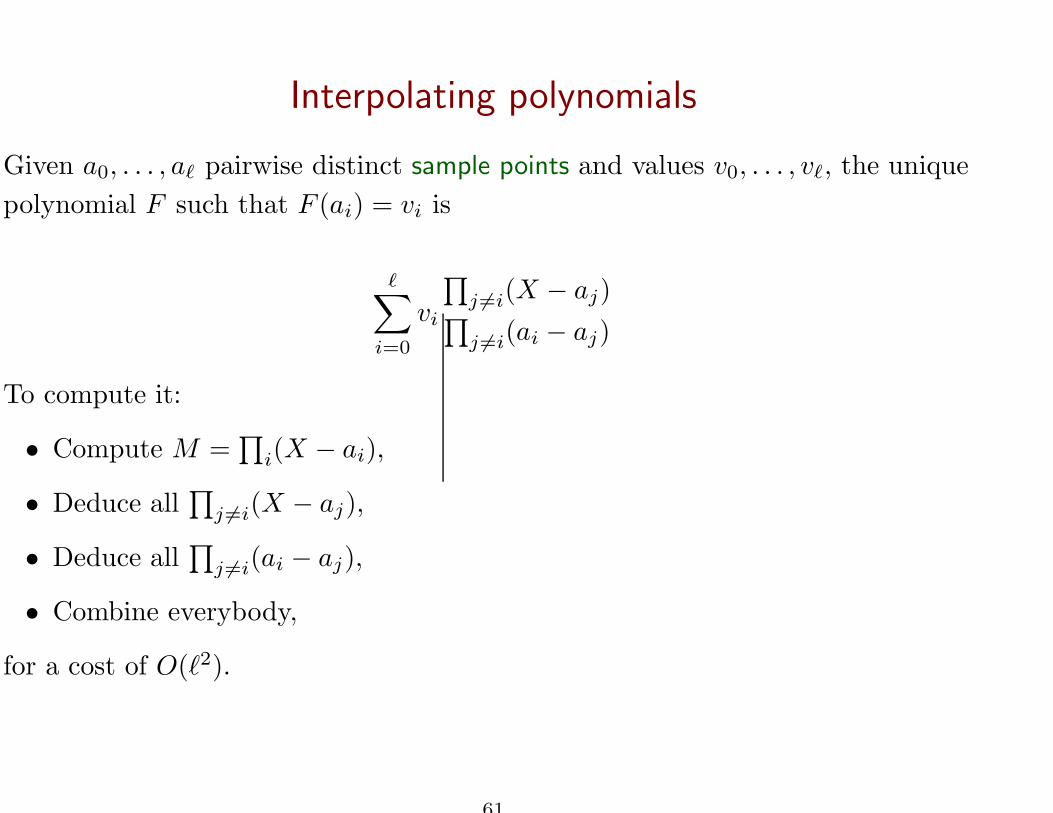
Given a0, . . . , aℓ pairwise distinct sample points and values v0, . . . , vℓ, the unique
polynomial F such that F (ai) = vi is
ℓ∑
i=0
vi
∏
j 6=i(X − aj)∏
j 6=i(ai − aj)
60
Interpolating polynomials
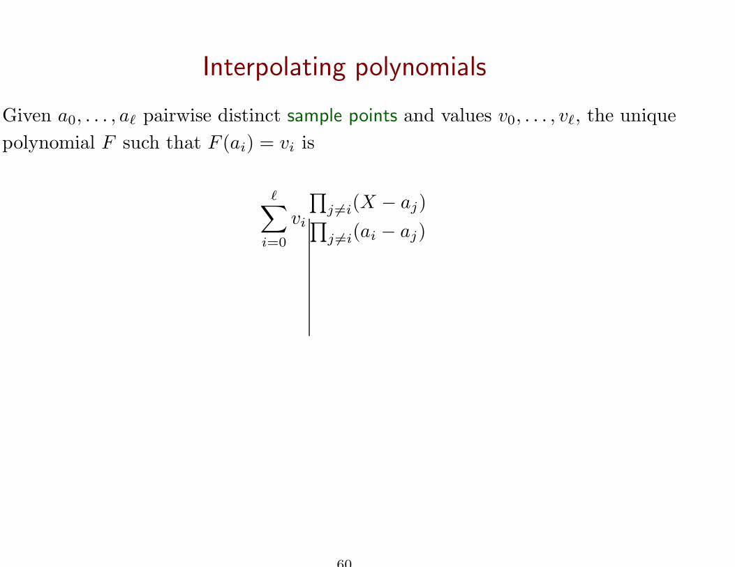
Given a0, . . . , aℓ pairwise distinct sample points and values v0, . . . , vℓ, the unique
polynomial F such that F (ai) = vi is
ℓ∑
i=0
vi
∏
j 6=i(X − aj)∏
j 6=i(ai − aj)
To compute it:
• Compute M =∏
i(X − ai),
• Deduce all∏
j 6=i(X − aj),
• Deduce all∏
j 6=i(ai − aj),
• Combine everybody,
for a cost of O(ℓ2).
61

Switching to fast algorithms
62
Speeding things up
Let M(d) denote the cost of polynomial multiplication in degree d:
• M(d) ∈ O(d2) for a naive algorithm
• M(d) ∈ O(d log d) using Fast Fourier Transform (if the field has roots of 1)
• M(d) ∈ O(d log d log log d) using Fast Fourier Transform in general.
Technically, we ask M(d + d′) ≥ M(d) + M(d′).
63
Speeding things up
Let M(d) denote the cost of polynomial multiplication in degree d:
• M(d) ∈ O(d2) for a naive algorithm
• M(d) ∈ O(d log d) using Fast Fourier Transform (if the field has roots of 1)
• M(d) ∈ O(d log d log log d) using Fast Fourier Transform in general.
Technically, we ask M(d + d′) ≥ M(d) + M(d′).
Using the fact that Euclidean division can be made in time O(M(d)), both parts
can be made faster:
• Euclid’s algorithm: divide-and-conquer and half-GCD techniques,
O(d2 × M(d) log(d))
• Interpolation using subproduct trees techniques.
O(M(d2) log(d))
64
FFT in a nutshell
Suppose you want to evaluate F (X) ∈ C[X ] at all N -roots of 1
1, exp2iπ
N, exp
4iπ
N, . . . , exp
2(N − 1)iπ
N,
with deg(F ) < N .
65
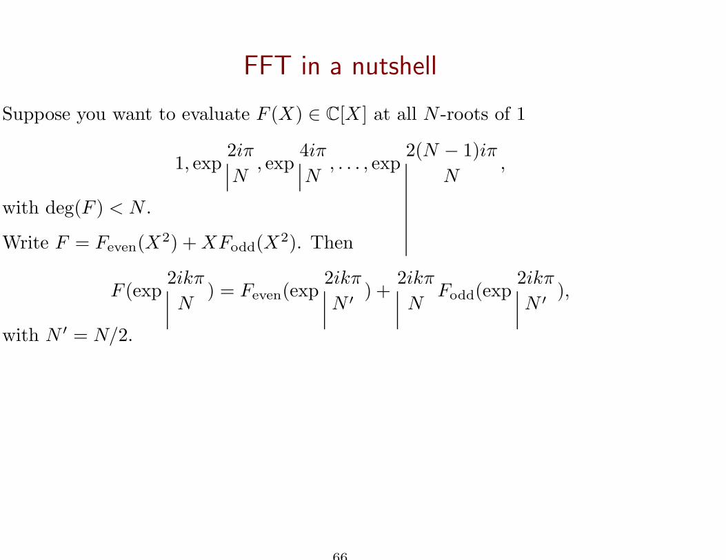
FFT in a nutshell
Suppose you want to evaluate F (X) ∈ C[X ] at all N -roots of 1
1, exp2iπ
N, exp
4iπ
N, . . . , exp
2(N − 1)iπ
N,
with deg(F ) < N .
Write F = Feven(X2) + XFodd(X2). Then
F (exp2ikπ
N) = Feven(exp
2ikπ
N ′) +
2ikπ
NFodd(exp
2ikπ
N ′),
with N ′ = N/2.
66
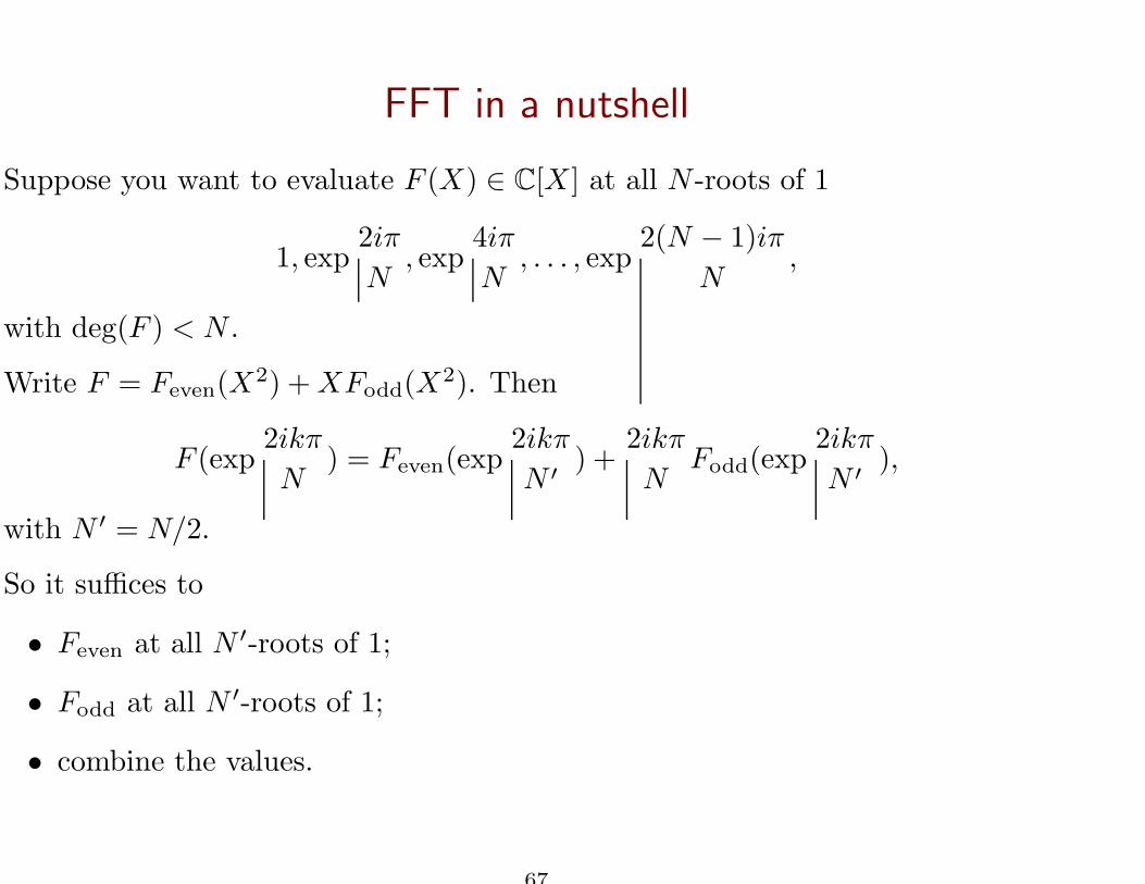
FFT in a nutshell
Suppose you want to evaluate F (X) ∈ C[X ] at all N -roots of 1
1, exp2iπ
N, exp
4iπ
N, . . . , exp
2(N − 1)iπ
N,
with deg(F ) < N .
Write F = Feven(X2) + XFodd(X2). Then
F (exp2ikπ
N) = Feven(exp
2ikπ
N ′) +
2ikπ
NFodd(exp
2ikπ
N ′),
with N ′ = N/2.
So it suffices to
• Feven at all N ′-roots of 1;
• Fodd at all N ′-roots of 1;
• combine the values.
67
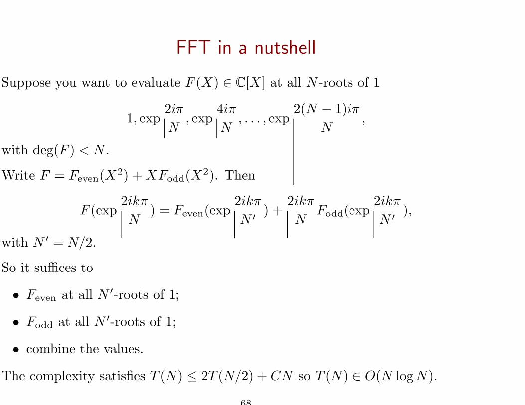
FFT in a nutshell
Suppose you want to evaluate F (X) ∈ C[X ] at all N -roots of 1
1, exp2iπ
N, exp
4iπ
N, . . . , exp
2(N − 1)iπ
N,
with deg(F ) < N .
Write F = Feven(X2) + XFodd(X2). Then
F (exp2ikπ
N) = Feven(exp
2ikπ
N ′) +
2ikπ
NFodd(exp
2ikπ
N ′),
with N ′ = N/2.
So it suffices to
• Feven at all N ′-roots of 1;
• Fodd at all N ′-roots of 1;
• combine the values.
The complexity satisfies T (N) ≤ 2T (N/2) + CN so T (N) ∈ O(N log N).
68
FFT in a nutshell
Proposition The inverse FFT can be performed for the same cost as the direct
FFT.
Corollary One can multiply F (X), G(X) ∈ C[X ], both of them having degree
< N , in O(N log N) operations
• Evaluate F and G at 2N -th roots of 1
• Multiply the values
• Do inverse-FFT to interpolate the product FG.
Extension to any field having “roots of unity”.
69
Towards a fast Euclidean algorithm
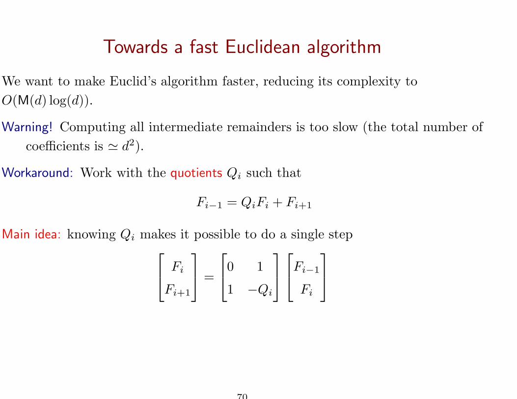
We want to make Euclid’s algorithm faster, reducing its complexity to
O(M(d) log(d)).
Warning! Computing all intermediate remainders is too slow (the total number of
coefficients is ≃ d2).
Workaround: Work with the quotients Qi such that
Fi−1 = QiFi + Fi+1
Main idea: knowing Qi makes it possible to do a single step
Fi
Fi+1
=
0 1
1 −Qi
Fi−1
Fi
70
Towards a fast Euclidean algorithm
We want to make Euclid’s algorithm faster, reducing its complexity to
O(M(d) log(d)).
Warning! Computing all intermediate remainders is too slow (the total number of
coefficients is ≃ d2).
Workaround: Work with the quotients Qi such that
Fi−1 = QiFi + Fi+1
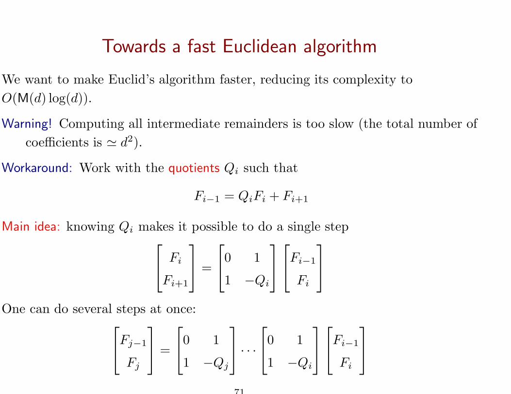
Main idea: knowing Qi makes it possible to do a single step
Fi
Fi+1
=
0 1
1 −Qi
Fi−1
Fi
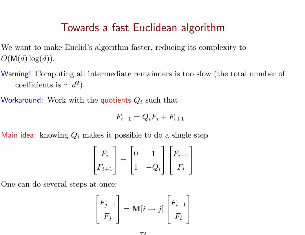
One can do several steps at once:
Fj−1
Fj
=
0 1
1 −Qj
· · ·
0 1
1 −Qi
Fi−1
Fi
71
Towards a fast Euclidean algorithm
We want to make Euclid’s algorithm faster, reducing its complexity to
O(M(d) log(d)).
Warning! Computing all intermediate remainders is too slow (the total number of
coefficients is ≃ d2).
Workaround: Work with the quotients Qi such that
Fi−1 = QiFi + Fi+1
Main idea: knowing Qi makes it possible to do a single step
Fi
Fi+1
=
0 1
1 −Qi
Fi−1
Fi
One can do several steps at once:
Fj−1
Fj
= M[i → j]
Fi−1
Fi
72
Half GCD: specifications and applications
Let F, G ∈ K[Y ] with d = deg F > deg G, and let
F1 = F, F2 = G, . . . , FN = 0
be the remainders met during Euclid’s algorithm.
73
Half GCD: specifications and applications
Let F, G ∈ K[Y ] with d = deg F > deg G, and let
F1 = F, F2 = G, . . . , FN = 0
be the remainders met during Euclid’s algorithm. There exists a unique ℓ such
that
deg(Fℓ−1) ≥ d/2 > deg(Fℓ).
74
Half GCD: specifications and applications
Let F, G ∈ K[Y ] with d = deg F > deg G, and let
F1 = F, F2 = G, . . . , FN = 0
be the remainders met during Euclid’s algorithm. There exists a unique ℓ such
that
deg(Fℓ−1) ≥ d/2 > deg(Fℓ).
The half-GCD algorithm compute the matrix M[2 → ℓ], so that
Fℓ−1
Fℓ
= M[2 → ℓ]
F1
F2
.
75
Half GCD: specifications and applications
Let F, G ∈ K[Y ] with d = deg F > deg G, and let
F1 = F, F2 = G, . . . , FN = 0
be the remainders met during Euclid’s algorithm. There exists a unique ℓ such
that
deg(Fℓ−1) ≥ d/2 > deg(Fℓ).
The half-GCD algorithm compute the matrix M[2 → ℓ], so that
Fℓ−1
Fℓ
= M[2 → ℓ]
F1
F2
.
• If Fℓ = 0, Fℓ−1 is the GCD,
76
Half GCD: specifications and applications
Let F, G ∈ K[Y ] with d = deg F > deg G, and let
F1 = F, F2 = G, . . . , FN = 0
be the remainders met during Euclid’s algorithm. There exists a unique ℓ such
that
deg(Fℓ−1) ≥ d/2 > deg(Fℓ).
The half-GCD algorithm compute the matrix M[2 → ℓ], so that
Fℓ−1
Fℓ
= M[2 → ℓ]
F1
F2
.
• If Fℓ = 0, Fℓ−1 is the GCD,
• Else, compute Fℓ+1 (to be sure that all degrees are < d/2), and continue with
Fℓ, Fℓ+1.
77
Extension to resultant computation
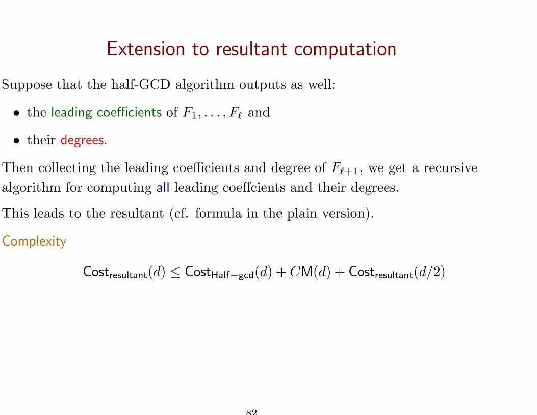
Suppose that the half-GCD algorithm outputs as well:
• the leading coefficients of F1, . . . , Fℓ and
• their degrees.
78
Extension to resultant computation
Suppose that the half-GCD algorithm outputs as well:
• the leading coefficients of F1, . . . , Fℓ and
• their degrees.
Then collecting the leading coefficients and degree of Fℓ+1, we get a recursive
algorithm for computing all leading coeffcients and their degrees.
79
Extension to resultant computation
Suppose that the half-GCD algorithm outputs as well:
• the leading coefficients of F1, . . . , Fℓ and
• their degrees.
Then collecting the leading coefficients and degree of Fℓ+1, we get a recursive
algorithm for computing all leading coeffcients and their degrees.
This leads to the resultant (cf. formula in the plain version).
80
Extension to resultant computation
Suppose that the half-GCD algorithm outputs as well:
• the leading coefficients of F1, . . . , Fℓ and
• their degrees.
Then collecting the leading coefficients and degree of Fℓ+1, we get a recursive
algorithm for computing all leading coeffcients and their degrees.
This leads to the resultant (cf. formula in the plain version).
Complexity
Costresultant(d) ≤ CostHalf−gcd(d)+O(M(d))+CostEuclidean division(d)+Costresultant(d/2)
81
Extension to resultant computation
Suppose that the half-GCD algorithm outputs as well:
• the leading coefficients of F1, . . . , Fℓ and
• their degrees.
Then collecting the leading coefficients and degree of Fℓ+1, we get a recursive
algorithm for computing all leading coeffcients and their degrees.
This leads to the resultant (cf. formula in the plain version).
Complexity
Costresultant(d) ≤ CostHalf−gcd(d) + CM(d) + Costresultant(d/2)
82
Extension to resultant computation
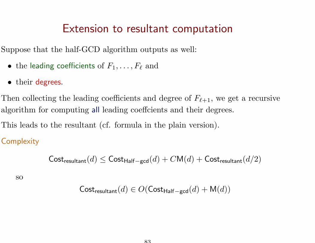
Suppose that the half-GCD algorithm outputs as well:
• the leading coefficients of F1, . . . , Fℓ and
• their degrees.
Then collecting the leading coefficients and degree of Fℓ+1, we get a recursive
algorithm for computing all leading coeffcients and their degrees.
This leads to the resultant (cf. formula in the plain version).
Complexity
Costresultant(d) ≤ CostHalf−gcd(d) + CM(d) + Costresultant(d/2)
so
Costresultant(d) ∈ O(CostHalf−gcd(d) + M(d))
83
The idea of half-GCD
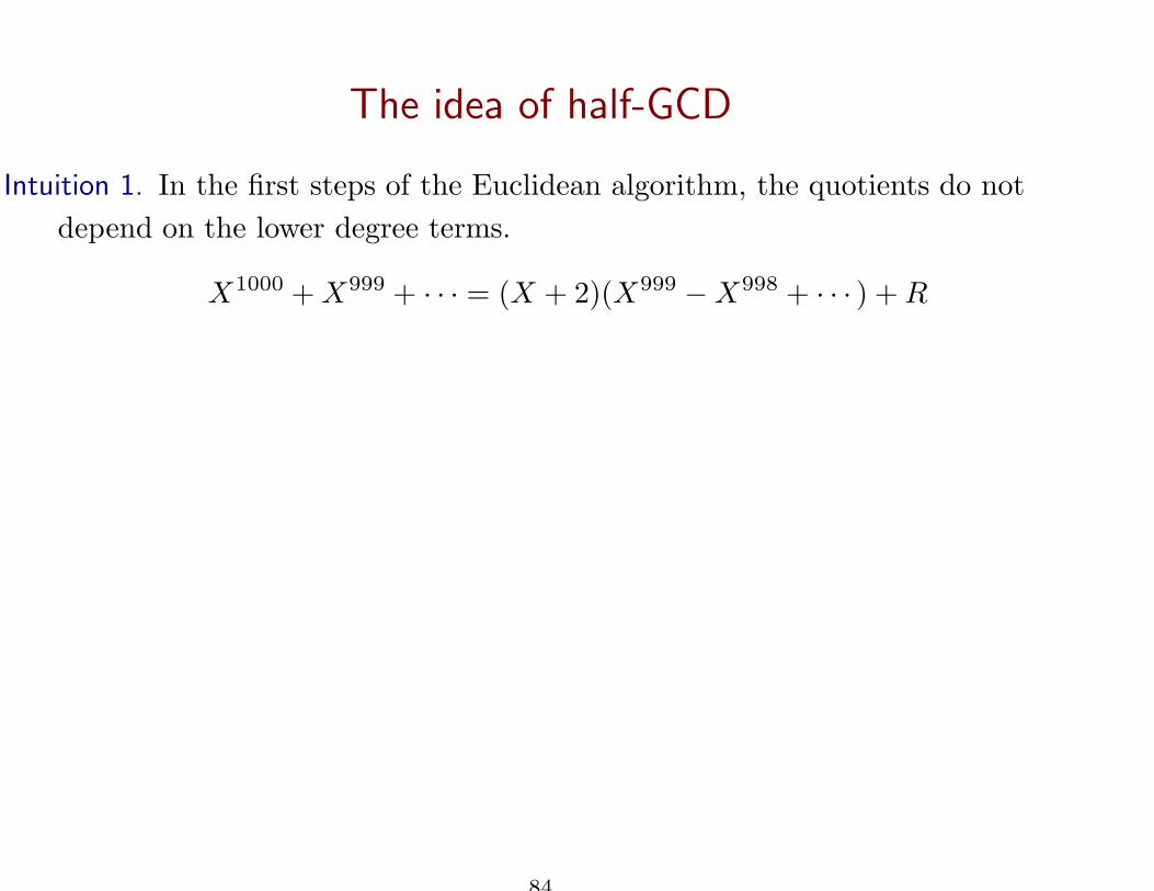
Intuition 1. In the first steps of the Euclidean algorithm, the quotients do not
depend on the lower degree terms.
X1000 + X999 + · · · = (X + 2)(X999 − X998 + · · · ) + R
84
The idea of half-GCD
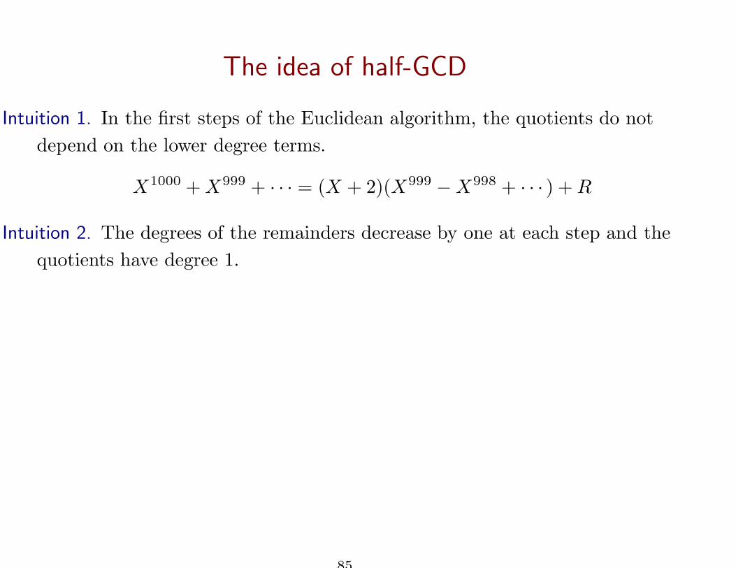
Intuition 1. In the first steps of the Euclidean algorithm, the quotients do not
depend on the lower degree terms.
X1000 + X999 + · · · = (X + 2)(X999 − X998 + · · · ) + R
Intuition 2. The degrees of the remainders decrease by one at each step and the
quotients have degree 1.
85
The idea of half-GCD
Intuition 1. In the first steps of the Euclidean algorithm, the quotients do not
depend on the lower degree terms.
X1000 + X999 + · · · = (X + 2)(X999 − X998 + · · · ) + R
Intuition 2. The degrees of the remainders decrease by one at each step and the
quotients have degree 1.
Hence, a transition matrix of degree ℓ yields remainders of degree ≃ d − ℓ.
86
The idea of half-GCD
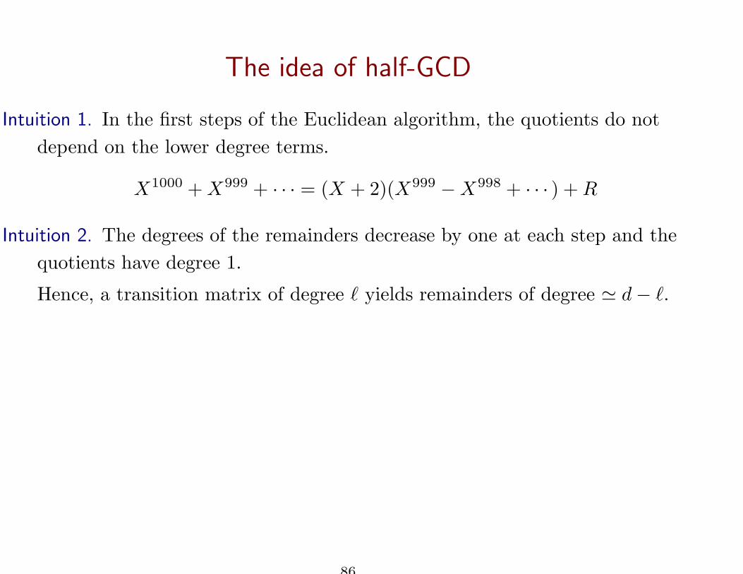
Intuition 1. In the first steps of the Euclidean algorithm, the quotients do not
depend on the lower degree terms.
X1000 + X999 + · · · = (X + 2)(X999 − X998 + · · · ) + R
Intuition 2. The degrees of the remainders decrease by one at each step and the
quotients have degree 1.
Hence, a transition matrix of degree ℓ yields remainders of degree ≃ d − ℓ.
Intuition 3. The half-GCD matrix of F1, F2 has entries of degrees ≃ d/2.
87
The idea of half-GCD
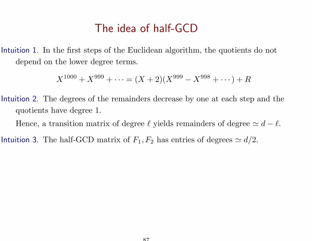
Intuition 1. In the first steps of the Euclidean algorithm, the quotients do not
depend on the lower degree terms.
X1000 + X999 + · · · = (X + 2)(X999 − X998 + · · · ) + R
Intuition 2. The degrees of the remainders decrease by one at each step and the
quotients have degree 1.
Hence, a transition matrix of degree ℓ yields remainders of degree ≃ d − ℓ.
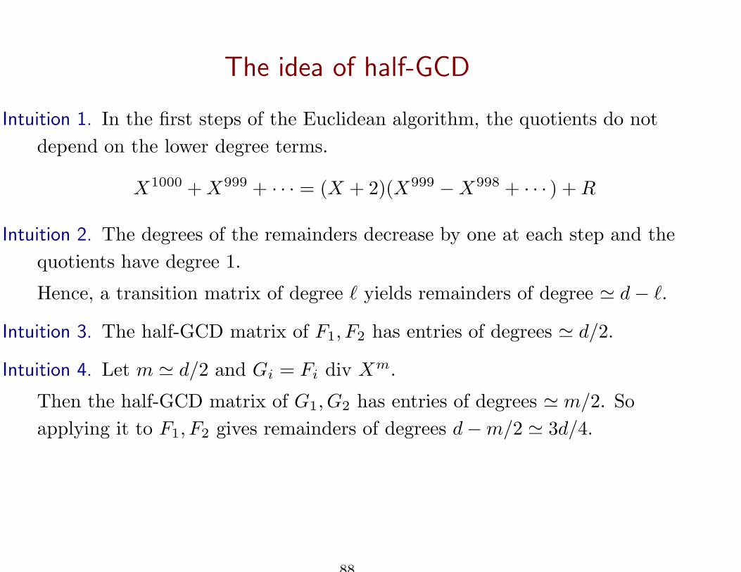
Intuition 3. The half-GCD matrix of F1, F2 has entries of degrees ≃ d/2.
Intuition 4. Let m ≃ d/2 and Gi = Fi div Xm.
Then the half-GCD matrix of G1, G2 has entries of degrees ≃ m/2. So
applying it to F1, F2 gives remainders of degrees d − m/2 ≃ 3d/4.
88
The half-GCD (sketch)
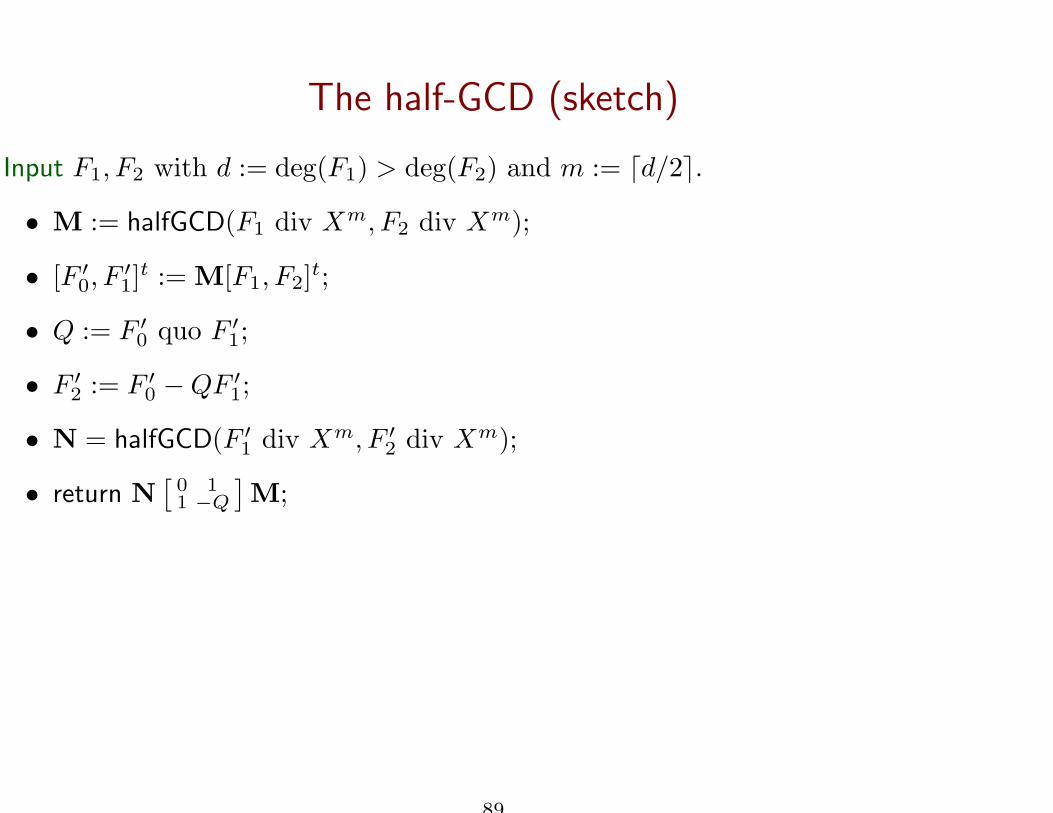
Input F1, F2 with d := deg(F1) > deg(F2) and m := ⌈d/2⌉.
• M := halfGCD(F1 div Xm, F2 div Xm);
• [F ′0, F
′1]
t := M[F1, F2]t;
• Q := F ′0 quo F ′
1;
• F ′2 := F ′
0 − QF ′1;
• N = halfGCD(F ′1 div Xm, F ′
2 div Xm);
• return N[
0 11 −Q
]M;
89
The half-GCD (sketch)
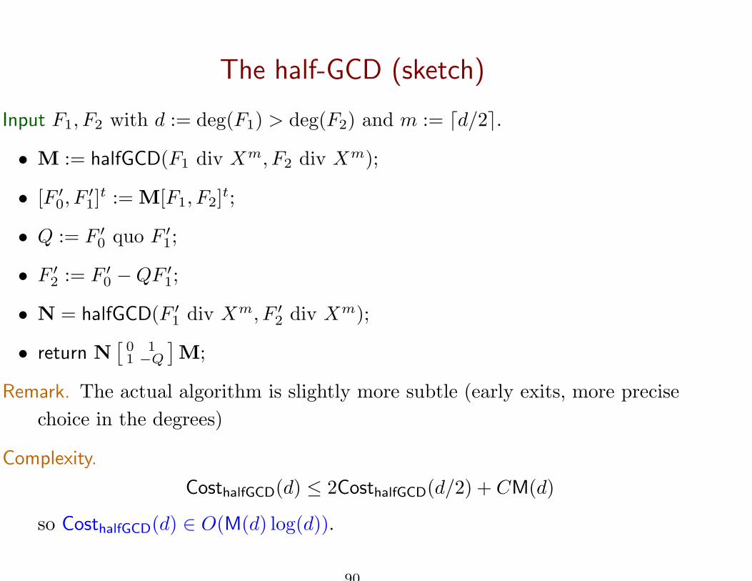
Input F1, F2 with d := deg(F1) > deg(F2) and m := ⌈d/2⌉.
• M := halfGCD(F1 div Xm, F2 div Xm);
• [F ′0, F
′1]
t := M[F1, F2]t;
• Q := F ′0 quo F ′
1;
• F ′2 := F ′
0 − QF ′1;
• N = halfGCD(F ′1 div Xm, F ′
2 div Xm);
• return N[
0 11 −Q
]M;
Remark. The actual algorithm is slightly more subtle (early exits, more precise
choice in the degrees)
Complexity.
CosthalfGCD(d) ≤ 2CosthalfGCD(d/2) + CM(d)
so CosthalfGCD(d) ∈ O(M(d) log(d)).
90
The half-GCD (sketch)
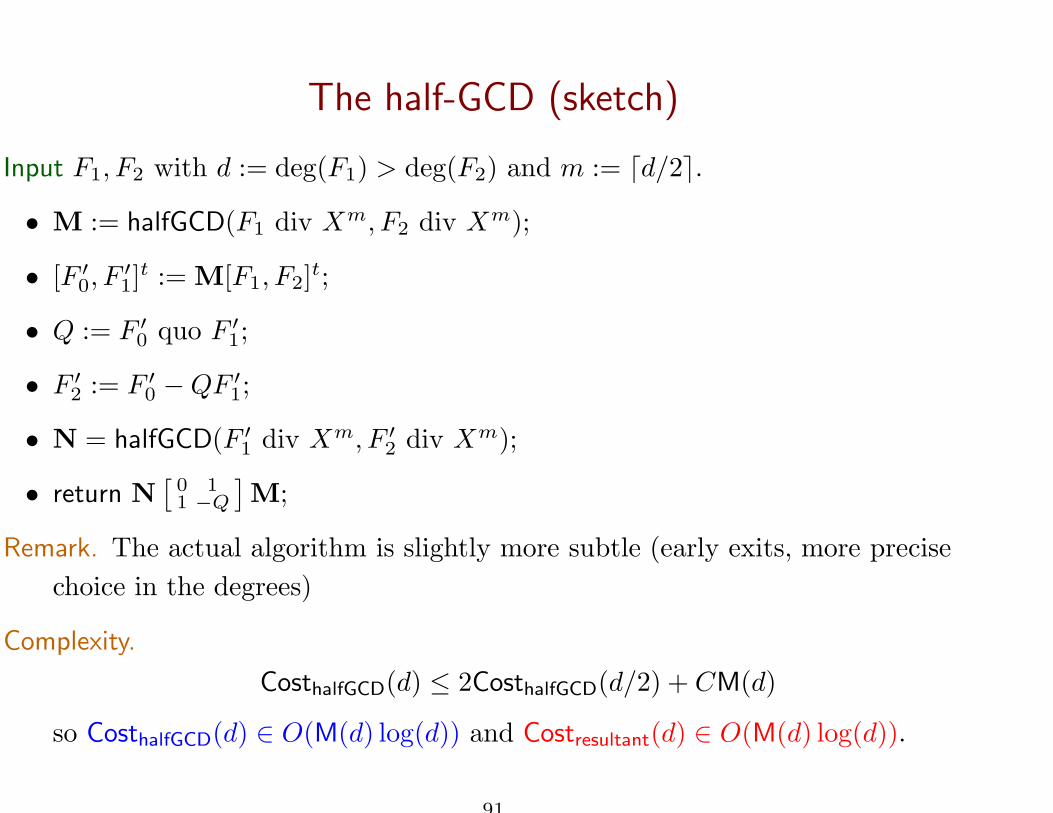
Input F1, F2 with d := deg(F1) > deg(F2) and m := ⌈d/2⌉.
• M := halfGCD(F1 div Xm, F2 div Xm);
• [F ′0, F
′1]
t := M[F1, F2]t;
• Q := F ′0 quo F ′
1;
• F ′2 := F ′
0 − QF ′1;
• N = halfGCD(F ′1 div Xm, F ′
2 div Xm);
• return N[
0 11 −Q
]M;
Remark. The actual algorithm is slightly more subtle (early exits, more precise
choice in the degrees)
Complexity.
CosthalfGCD(d) ≤ 2CosthalfGCD(d/2) + CM(d)
so CosthalfGCD(d) ∈ O(M(d) log(d)) and Costresultant(d) ∈ O(M(d) log(d)).
91


