
Analysis of a model of elastic plastic mixtures(“Prandtl-Reuss-mixtures”)
By Josef Malek and Jens Frehse
Krakow 2012

Introduction KMRS model Prandtl-Reuss Prandtl-Reuss mixtures Regularity techniques
Outline
Introduction
KMRS model
Prandtl-Reuss
Prandtl-Reuss mixtures
Regularity techniques
Introduction KMRS model Prandtl-Reuss Prandtl-Reuss mixtures Regularity techniques
We refer to a paper
J. Kratochvıl, J. Malek, K.R. Rajagopal and A.R. Srinivasa:Modelling of the response of elastic plastic materials treated asmixture of hard and soft regions, ZAMP 55 (2004), 500-518
and to
Phd-Thesis of Luba Khasina
adviced by Kratochvıl-Malek-Frehse, where first steps are done toformulate the model of KMRS in the framework of Sobolev spacesnad variational inequalities.

Introduction KMRS model Prandtl-Reuss Prandtl-Reuss mixtures Regularity techniques
KMRS consider a body Ω consisting of soft and hard material andloading.During the loading process, soft material is assumed to beperfectly elastic plastic, the hard material is assumed to satisfy acertain hardening rule in the non elastic region.The beautiness of the theory consists in the fact, that no artificialinternal variables enter, the history of the plastic deformation ofthe soft material replaces the internal variable.

Introduction KMRS model Prandtl-Reuss Prandtl-Reuss mixtures Regularity techniques
Purpose of the present talk
Presenting a mathematical formulation in the framework ofquasi-variational inequalities and Sobolev spaces.The theory turns out to be very similar to the Prandtl-Reuss-lawfor single materials; all known regularity results hold also for themixture model.
Introduction KMRS model Prandtl-Reuss Prandtl-Reuss mixtures Regularity techniques
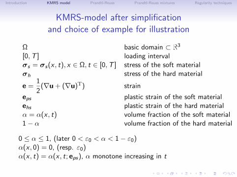
KMRS-model after simplificationand choice of example for illustration
Ω basic domain ⊂ R3
[0,T ] loading intervalσs = σs(x , t), x ∈ Ω, t ∈ [0,T ] stress of the soft materialσh stress of the hard material
e =1
2(∇u + (∇u)T) strain
eps plastic strain of the soft materialehs plastic strain of the hard materialα = α(x , t) volume fraction of the soft material1− α volume fraction of the hard material
0 ≤ α ≤ 1, (later 0 < ε0 < α < 1− ε0)α(x , 0) = 0, (resp. ε0)α(x , t) = α(x , t; eps), α monotone increasing in t
Introduction KMRS model Prandtl-Reuss Prandtl-Reuss mixtures Regularity techniques
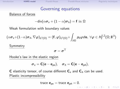
Governing equationsBalance of forces
−div(ασs + (1− α)σh) = f in Ω
Weak formulation with boundary values
(ασs+(1−α)σh,∇ϕ)L2(Ω) = (f,ϕ)L2(Ω)+
∫∂Ω
p0ϕdo, ∀ϕ ∈ H1,2Γ (Ω;R3)
Symmetry
σ = σT
Hooke’s law in the elastic region
σs = C(e− eps), σh = C(e− eph),
C elasticity tensor, of course different Cs and Ch can be used.Plastic incompressibility
trace eps = trace eph = 0.
Introduction KMRS model Prandtl-Reuss Prandtl-Reuss mixtures Regularity techniques
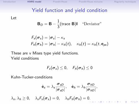
Yield function and yield condition
Let
BD = B− 1
3(trace B)I “Deviator”
Fs(σs) = |σs | − κsFh(σh) = |σh| − κh(t), κh(t) = κh(t, eps)
These are v Mises type yield functions.Yield conditions
Fs(σs) ≤ 0, Fh(σh) ≤ 0
Kuhn-Tucker-conditions
es = λsσsD
|σsD |, eh = λh
σhD
|σhD |,
λs , λh ≥ 0, λsFs(σs) = 0, λhFh(σh) = 0.
Introduction KMRS model Prandtl-Reuss Prandtl-Reuss mixtures Regularity techniques
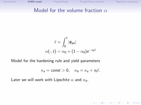
Model for the volume fraction α
` =
∫ t
0|eps |
α(·, t) = α0 + (1− α0)e−c0`
Model for the hardening rule and yield parameters
κs = const > 0, κh = κs + r0`.
Later we will work with Lipschitz α and κh.
Introduction KMRS model Prandtl-Reuss Prandtl-Reuss mixtures Regularity techniques
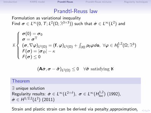
Prandtl-Reuss lawFormulation as variational inequalityFind σ ∈ L∞(0,T ; L2(Ω;R3×3)) such that σ ∈ L∞(L2) and
K
σ(0) = σ0
σ = σT
(σ,∇ϕ)L2(Ω) = (f,ϕ)L2(Ω) +∫∂Ω p0ϕdo, ∀ϕ ∈ H1,2
Γ (Ω;R3)
F (σ) = |σD | − κF (σ) ≤ 0
(Aσ,σ − σ)L2(Ω) ≤ 0 ∀σ satisfying K
Theorem
∃ unique solutionRegularity results: σ ∈ L∞(L2+δ), σ ∈ L∞(H1,2
loc ) (1992),σ ∈ H1/2,2(L2) (2011)
Strain and plastic strain can be derived via penalty approximation.
Introduction KMRS model Prandtl-Reuss Prandtl-Reuss mixtures Regularity techniques
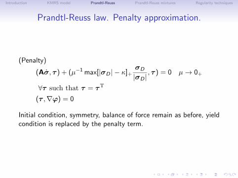
Prandtl-Reuss law. Penalty approximation.
(Penalty)
(Aσ, τ ) + (µ−1 max[|σD | − κ]+σD
|σD |, τ ) = 0 µ→ 0+
∀τ such that τ = τT
(τ ,∇ϕ) = 0
Initial condition, symmetry, balance of force remain as before, yieldcondition is replaced by the penalty term.
Introduction KMRS model Prandtl-Reuss Prandtl-Reuss mixtures Regularity techniques
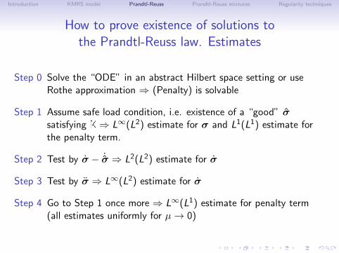
How to prove existence of solutions tothe Prandtl-Reuss law. Estimates
Step 0 Solve the “ODE” in an abstract Hilbert space setting or useRothe approximation ⇒ (Penalty) is solvable
Step 1 Assume safe load condition, i.e. existence of a “good” σsatisfying K⇒ L∞(L2) estimate for σ and L1(L1) estimate forthe penalty term.
Step 2 Test by σ − ˙σ ⇒ L2(L2) estimate for σ
Step 3 Test by σ ⇒ L∞(L2) estimate for σ
Step 4 Go to Step 1 once more ⇒ L∞(L1) estimate for penalty term(all estimates uniformly for µ→ 0)
Introduction KMRS model Prandtl-Reuss Prandtl-Reuss mixtures Regularity techniques
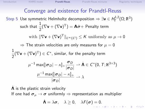
Converge and existence for Prandtl-Reuss
Step 5 Use symmetric Helmholtz decomposition ⇒ ∃v ∈ H1,2Γ (Ω;R3)
such that1
2(∇v + (∇v)T) = Aσ+ Penalty term
with ‖∇v + (∇v)T‖L∞(L1) ≤ K uniformly as µ→ 0
⇒ The strain velocities are only measures for µ = 0
1
2(∇v + (∇v)T) ∈ C ∗, similar, for the penalty term
µ−1 max[|σD | − κ]+σD
|σD | Λ ∈ C ∗(0,T ;R3×3)
µ−1 max[|σD | − κ]+|σD |
λ
Λ is the plastic strain velocityIf one had σµ → σ uniformly ⇒ representation as multiplier
Λ = λσ, λ ≥ 0, λF (σ) = 0.

Introduction KMRS model Prandtl-Reuss Prandtl-Reuss mixtures Regularity techniques
Theorem
σµ → σ,σ solution of the Prandtl-Reuss variational inequality and
1
2(∇v + (∇v)T) = Aσ + Λ.
A similar procedure can be done for the mixture MDE model ofKMRS.
Introduction KMRS model Prandtl-Reuss Prandtl-Reuss mixtures Regularity techniques
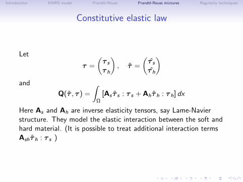
Constitutive elastic law
Let
τ =
(τ s
τ h
), τ =
(τ s
τ h
)and
Q(τ , τ ) =
∫Ω
[As τ s : τ s + Ahτ h : τ h] dx
Here As and Ah are inverse elasticity tensors, say Lame-Navierstructure. They model the elastic interaction between the soft andhard material. (It is possible to treat additional interaction termsAshτ h : τ s )
Introduction KMRS model Prandtl-Reuss Prandtl-Reuss mixtures Regularity techniques
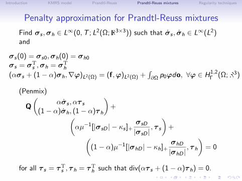
Penalty approximation for Prandtl-Reuss mixtures
Find σs ,σh ∈ L∞(0,T ; L2(Ω;R3×3)) such that σs , σh ∈ L∞(L2)and
σs(0) = σs0,σh(0) = σh0
σs = σTs ,σh = σT
h
(ασs + (1− α)σh,∇ϕ)L2(Ω) = (f,ϕ)L2(Ω) +∫∂Ω p0ϕdo, ∀ϕ ∈ H1,2
Γ (Ω;R3)
(Penmix)
Q
(ασs , ατ s
(1− α)σh, (1− α)τ h
)+(
αµ−1[|σsD | − κs ]+σsD
|σsD |, τ s
)+(
(1− α)µ−1[|σhD | − κh]+σhD
|σhD |, τ h
)= 0
for all τ s = τTs , τ h = τT
h such that div(ατ s + (1− α)τ h) = 0.
Introduction KMRS model Prandtl-Reuss Prandtl-Reuss mixtures Regularity techniques
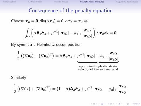
Consequence of the penalty equation
Choose τ h = 0, div(ατ s) = 0, ατ s = τ 0 ⇒∫Ω
(αAsσs + µ−1[|σsD | − κs ]+
σsD
|σsD |
): τ 0dx = 0
By symmetric Helmholtz decomposition
1
2
((∇us) + (∇us)T
)= αAsσs + µ−1[|σsD | − κs ]+
σsD
|σsD |︸ ︷︷ ︸approximate plastic strainvelocity of the soft material
Similarly
1
2
((∇uh) + (∇uh)T
)= (1− α)Ahσh + µ−1[|σhD | − κh]+
σhD
|σhD |

Introduction KMRS model Prandtl-Reuss Prandtl-Reuss mixtures Regularity techniques
Theorem
Assume α, κh Lipschitz, Q positively definite and smooth data.Assume a safe load condition with smooth stresses σs and σh. Let0 ≤ ε0 ≤ α ≤ 1− ε0. Then
1. The solutions σns ,σ
nh are uniformly bounded in the norms
L∞(L2), L∞(L2+δ),H1,∞(L2). Furthermore σ ∈ H1/2(L2).
2. The partial strain velocities and the partial plastic strainvelocities are bounded in L∞(L1).
3. The approximate stresses converge weaklyσns σs ,σ
nh σh (µ→ 0+) in H1,2(L2) ∩ L2(H1,2
loc ).

Introduction KMRS model Prandtl-Reuss Prandtl-Reuss mixtures Regularity techniques
Theorem (continuation)
The limit satisfies the variational inequality
Q
((ασs
(1− α)σh
),
(α(σs − τ s)
(1− α)(σh − τ h)
))≤ 0 (V)
with respect to the yield conditions and the balance of forcesdefining the convex set.
Since in the application α = α(t, x ;σs ,σh) and similar κh,inequality (V) is a quasi-variational inequality.
Introduction KMRS model Prandtl-Reuss Prandtl-Reuss mixtures Regularity techniques
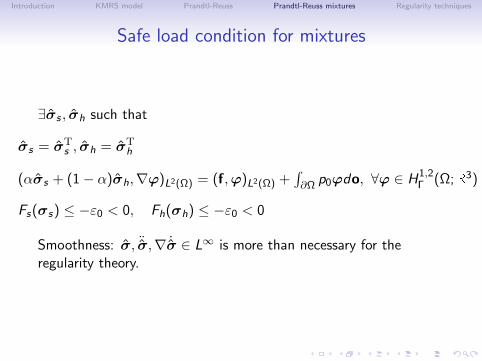
Safe load condition for mixtures
∃σs , σh such that
σs = σTs , σh = σT
h
(ασs + (1− α)σh,∇ϕ)L2(Ω) = (f,ϕ)L2(Ω) +∫∂Ω p0ϕdo, ∀ϕ ∈ H1,2
Γ (Ω;R3)
Fs(σs) ≤ −ε0 < 0, Fh(σh) ≤ −ε0 < 0
Smoothness: σ, ¨σ,∇ ˙σ ∈ L∞ is more than necessary for theregularity theory.
Introduction KMRS model Prandtl-Reuss Prandtl-Reuss mixtures Regularity techniques
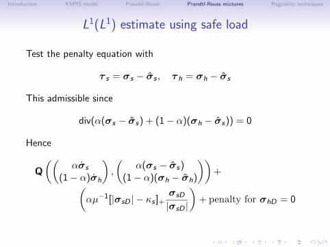
L1(L1) estimate using safe load
Test the penalty equation with
τ s = σs − σs , τ h = σh − σs
This admissible since
div(α(σs − σs) + (1− α)(σh − σs)) = 0
Hence
Q
((ασs
(1− α)σh
),
(α(σs − σs)
(1− α)(σh − σh)
))+(
αµ−1[|σsD | − κs ]+σsD
|σsD |
)+ penalty for σhD = 0
Introduction KMRS model Prandtl-Reuss Prandtl-Reuss mixtures Regularity techniques
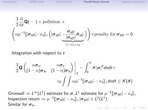
1
2
d
dtQ(· · · ) + pollution +(
αµ−1[|σsD |−κs ]+(|σsD | −
σsD
|σsD |σsD︸ ︷︷ ︸
≥−κs+ε0
))+penalty for σhD = 0
Integration with respect to t
1
2Q
(ασs , ασs
(1− α)σh, (1− α)σh
) ∣∣∣∣∣T
−∫ T
0K |σ|2dxdt+
ε0
∫ ∫αµ−1[|σsD | − κs ]+dxdt ≤ K (σ)
Gronwall ⇒ L∞(L2) estimate for σ, L1 estimate for µ−1[|σsD | − κs ]+Inspection return ⇒ µ−1[|σsD | − κs ]+|σsD | ∈ L1(L1)Similar for σh.
Introduction KMRS model Prandtl-Reuss Prandtl-Reuss mixtures Regularity techniques
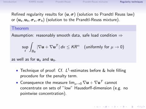
Refined regularity results for (u,σ) (solution to Prandtl Reuss law)or (us ,uh,σs ,σh) (solution to the Prandtl-Reuss mixture).
Theorem
Assumption: reasonably smooth data, safe load condition ⇒
supt
∫BR
|∇u +∇uT | dx ≤ KRα (uniformly for µ→ 0)
as well as for us and uh.
• Technique of proof: Cf. L1-estimates before & hole fillingprocedure for the penalty term.
• Consequence the measure limµ→0∇u +∇uT cannotconcentrate on sets of ”low” Hausdorff-dimension (e.g. nopointwise concentration).
Introduction KMRS model Prandtl-Reuss Prandtl-Reuss mixtures Regularity techniques
Theorem
Assumption as before, Ω0 b Ω,
supt
∫Ω0
|∇σ|2 dx ≤ K .
• Technique of proof: Difference quotient technique. Thepollution terms due to u give trouble since ∇u +∇uT isestimated only in L1.

Introduction KMRS model Prandtl-Reuss Prandtl-Reuss mixtures Regularity techniques
Boundary differentiability:Let Dτ be the tangential derivative at the boundary.
• Malek, JF ⇒ Dτσ ∈ L2 up to the boundary for n = 2, Ωcircle or cirlce\smaller circles.
• Bulicek, Malek, JF ⇒ Dτσ ∈ L2 for n ≥ 3, Ω circle orcirlce\smaller concentric circles.
• Seregin: Normal derivatives to certain approximations areunbounded, Ω =circle.
These results are published for Hencky’s law but hold forPrandtl-Reuss-problem and Prandtl-Reuss-mixtures as well.
Introduction KMRS model Prandtl-Reuss Prandtl-Reuss mixtures Regularity techniques
Fractional differentiability for σ, σh, σs .
Theorem
σ, σh, σs have fractional derivatives in the sense of Besov spacesin time direction of order 1
2 − δ, in space direction (interiorregularity) of order 1
6 − δ. This is claimed in the limit µ = 0.
• Proof: Use the function h−1(σ(t + s)− σ(t)) as atestfunction and perform h−1
∫ds. The spatial derivatives are
obtained via cross interpolation.

Introduction KMRS model Prandtl-Reuss Prandtl-Reuss mixtures Regularity techniques
Dziekuje za uwage.
Thank you for your attention.


