Analytical approach to probabilistic prediction of voltage sags on transmission networks
Y.S. Lim and G. Strbac \
Abstract: Quantification of voltage sags at a location of interest is the basic requirement for assessing the compatibility between equipment and electrical supply. An analytical method is described that has been developed to determine the probability density functions of voltage sags caused by three phase faults across the network. The method takes into account the impact of fault positions along transmission circuits and patterns of generation associated with the corresponding load demands on the voltage sag profiles. The developed algonthm is applied to the IEEE 24bus reliability test system to verify the technique and illustrate its application.
1 Introduction
Power quality is an issue conceming a variety of power system 'disturbances, ranging from intermittent voltage surges to harmonic distortions. Generally, it is manifested as voltage, current or frequency deviation, causing failure or malfunction of customer equipment [I]. The revitalisation of industry with electronically controlled equipment (which is more sensitive to deviations in the supply voltage than its electromechanical predecessors) is becoming increasingly concerned with various power quality issues.
Voltage sags are one of the central power quality problems faced by many industrial customers [2]. Voltage sags are short-duration (typically 0.5 to 30 cycles) [l] reductions in RMS voltage. They may be accompanied by phase-angle jumps caused by faults on the power system or the starting of a large machne. Much equipment used in modern industrial plants including process controllers, programmable logic controllers, adjustable speed drivers, robotics is sensitive to voltage sags. It is not uncommon for voltage sags to trip sensitive equipment, causing affected industrial customers to suffer great financial loss.
Electric utilities and end users of electrical power are becoming increasingly concerned about the quality of electric power. Considerable efforts are being made to understand, quantify and minimise the damaging impact of voltage sags on equipment. The procedures of assessing the compatibility between the equipment and supply are as follows:
Obtain system performance: information must be obtained on the system performance for the specific supply point; that is the expected number of voltage sags with different characteristics. There are various ways to obtain this information, such as monitoring the supply for several months or years. or predicting the supply performance.
~ ~~ ~~
,i> IEE. 2002 I€€ Proceedimg.s online no. 2W2W8 Dol: lO.I049/ipgtd2W2W08 Paper firs1 received 13th July 2W and in revired form 11th M q 2001 The authors arc with the Depanment of Engineeting and Electronics. UMIST. BIB-Fenanti Building. P.O. Box 88. Manchester MbO IQD. UK
I€€ Pnx.-Gmmr. Tr<mm Dislrib.. Vu/. i4Y. No. 1. Jonion. ZOO2
(ii) Obtain equipment voltage tolerance: information has to be obtained on the behaviour of the piece of equipment for various voltage sags. This information could be obtained from the equipment manufacturers or by performing tests on the equipment. Determine the expected impact in terms of how often the piece of equipment is expected to trip per year, and the financial consequences: based on the outcome of such a study, decisions regarding the supply arrangements could be made.
(iii)
As mentioned above, the system performance can either be monitored or predicted, or we can opt for a combination of the two approaches. It is, however, important to recognise that it may often be very time-consuming and costly to monitor the system performance; the characteristics of the disturbances need to be identified in a significant length of time, in order to obtain reasonable accuracy of the results. As discussed elsewhere [2], a period of 30 years would be required to obtain statistically significant results for an event that occurs once a month. Hence numerical techniques become vital for practical evaluation of voltage sag characteristics.
Two stochastic prediction methods have been discussed [2]: fault positions and critical distance. The basic principle OT the critical distance method is based on the concept of potential divider, which is only appli- cable to a radial network. The method cannot be used to deal with a complicated meshed network. Hence the applicability of the critical distance method is rather limited. As for the fault positions method, several positions on the network are chosen, and the voltage sag performance is then determined by introducing faults on the chosen points to simulate the occurrence of faults on the system. As faults may occur anywhere within the system, it may not be sufficient to simulate the occurrence of faults by just introducing the faults at pre- defined positions.
In this paper, we propose an analytical method that can be used to predict the severity and number of voltage sags at a bus of interest, taking into account the probabilistic nature of fault occurrence across the complicated meshed network, accompanied by the variation of generation patterns. A full statistical description of voltage sags, given in the form of a probability density function (PDF), is
7
determined by closed-form equations derived from the faultcalculation procedures proposed previously [3]. The method is particularly useful when an approximate voltage sag assessment on large networks is required, and it can he easily applied to study the impact of various system conditions and future expansion plans. The method is developed to deal with the worst voltage-sag scena&s caused by symmetrical three-phase faults. For the con- sideration of unbalanced faults, further work would need ty be carried out. I
L '3
2 Derivation of probability density function of voltage sags
n e basic concept of probabilistic characterisation of voltage sags is presented. First, simple expressions for voltage sags are derived using the network impedance matrix (Z-bus matrix), used in conventional fault calcula- tions. The expression for calculating the PDFs of voltage sags as a function of distributions of faults on a transmission line is then derived.
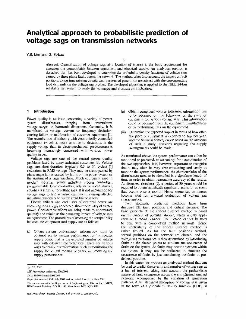
2.7 position An example of an electrical system (shown in Fig. 1) is employed to derive the expression for qualifying voltage sags. The network consists of n busbars with busbars k , j and m, as highlighted in Fig. I . Busbar In .is selected to represent the location at which sensitive equipment is connected, and thus an expression of voltage sag will he derived for that hushar
The change in voltage at husbar m, due to a three-phase
Calculation of voltage sag for given fault
[2, 41.
fault at busbar k, is given by
A v, = -z&Ik (1)
where A V,,, is the voltage sag during the fault at hushar k; Z,, is the transfer element that corresponds to busbars m and k; and Ik is the fault current at busbar k.
Eqn. 1 is obtained from a more general matrix equation, which enables the calculation of voltage sags at all busbars .~ due to a fault at busbar k:
O1 z/ ] . . . Z l k ... z i m . . . z], ... z].
z,, . . . Z& . . . z, . . . z, . . . z,
Z,] . . . Z& . . . z,, . . . Z,j . . . z,,
z,, . . . z, . . . zj, . . . z j j . . . Zj"
z.1 . . . Znk . . . z" . . . znj . . . z,
The fault current lk is calculated by
G Ik = - zkk
where 5' is the pre-fault voltage at hushar k; and Zkk is the driving element that corresponds to the diagonal element kk of the busbar impedance matrix.
8
Thus, the voltage at the husbar of interest during the fault V,,, can be expressed as
where VL is the pre-fault voltage at busbar m. Following the conventional assumption of neglecting the
pre-fault flows, the pre-fault voltages at all busbars are assumed to the 1 p.u. Hence, eqn. 4 can be simplified as
( 5 ) ZVlk v, = 1 -- Z&
Eqn. 5 is used to calculate voltage V,,, at hushar m, given that the fault occurs at bushar k.
In order to study the impact of the fault positions, and also the distribution of faults along the transmission circuit on voltage sags, the above expression needs to be general- ised. As shown in Fig. 2, an additional node p is placed at the location at which the fault occurs. Following the fault calculation procedure, the transfer and driving elements that correspond to the fault position p on line k-j can be calculated.
P 1 - 1 I
k I
1
I
/ - ' h i I
The expressions for transfer element Z , , and the driving element Z,,,,, respectively, are [3]
z,, = (1 - X)Z& + x z , j
z,,, = (1 - X)>Zkk + PZ,J + 2X( 1 - X)Z, + A( 1 - X)z,
(6)
(7) where Z,,* is the transfer impedance corresponding to husban m and k; Z!, is the transfer impedance correspond- ing to busbars m and j ; Zkj is the transfer impedance corresponding to busbars k and j ; Zkk is the driving impedance corresponding to busbar k; Z, is the driving impedance corresponding to hushar j ; and zkj is the impedance of transmission line k-j.
IEEProc.-Gene+ T r a m Olitrrb. Yo/. 149, No. 1. JmlunuuryZWZ
Note that eqns. 6 and 7 are both expressed in terms of variable 2, which defined the fault position:
(8) A = - Lkp O<X<l
where LIP is the distance between node k and position p; and Lkj is the length of transmission line k-j.
Parameter 1. moves from 0 to 1 as the point p moves from busbar k to busbarj.
Finally, the expression for voltage V,,, at busbar m, due to a fault position p on line k-j, is obtained by substituting eqns. 6 and 7 in eqn. 5:
v, = 1
L k j
- (1 - X)Z,, + Xz,j
(1 - A) z, + PZ,? + 2X( 1 - X)Z, + A ( 1 - X ) Z k j
(9)
2
2.2 Evaluation of PDF of voltage sags due to random distribution of faults along transmission lines Note that, in eqn. 9, parameter I. (which establishes the position of the fault along the transmission circuit) is a random variable, and hence V, is a random variable. The main question is how to determine the PDF of voltage V,,,. e.g. f l Vm), given the expression that describes the relation- ship between the two random variables V,, and ). (eqn. 9), and the PDF of 1, e.g. ~(1). Principle findings of probability theory [5, 61 offer the following formulae:
In order to calculated the derivative IdX/dV,I, eqn. 9 is used to express 2. in terms of V,,,:
- ( & E - E + E ) f J A “ V , +E”V, i C” 2(AVm - A )
A = [ Hence
- 1 - 2 ( A V , -A)’ J
complexity of this calculation does not depend on the nature of the distribution go.), as this distribution was not a part of the derivation in eqn. 12. Therefore, the calculations of the PDF can ,h performed with any form of g ( l ) , as indicated in eqn. 10.
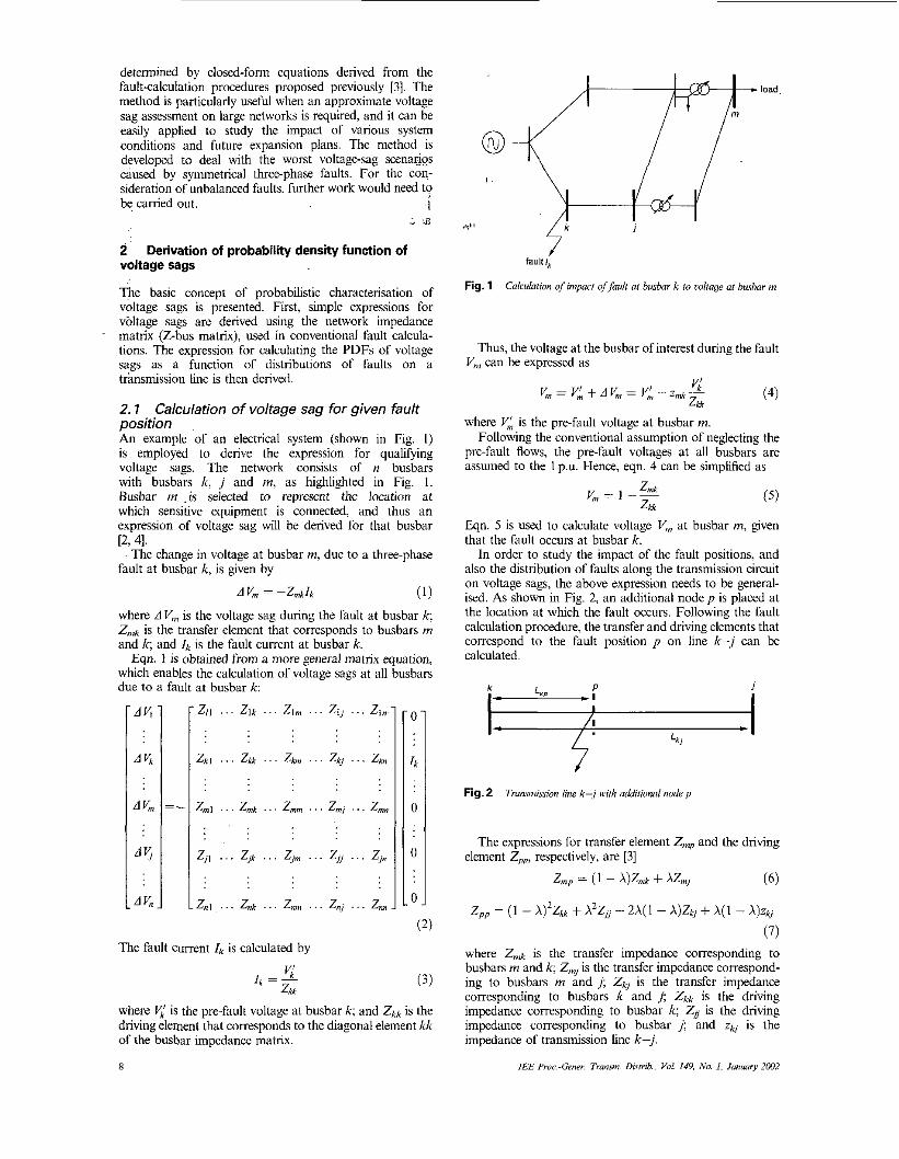
A two-busbar simple network (shown in Fig. 3) is used to illustrate the application, from which the PDF of the Goltage sag at busbar 4 is derived. Without a loss of ‘generality, in the folldking analysis, we assume that the faults are uniformly distributed along the transmission line, as described in Fig. 4.
j0.3 I 2
In this case, we assume that
g ( 4 = 1 (14) Substituting eqn. 14 in eqn. I O yields
The busbar impedance matrix that corresponds to the network is given by
By using eqn. 9, we obtain a simple relationship:
(17) 0.1
0.1 + 0.3X K = l - A f O
where A=Zkk+Zj-2Zb-zb; B=Zj-2Zkk-2zk,-~,; C=Z& D=Z,*; E=z ,-z,,*; A“ = p - 4AC; B“ = 2BE + 8 A C - 4 A D - 2 g a n d = p + 4 A D + 9 - BE - 4 A C .
Note that for 05x5 1 voltage V, at busbar 1 varies within the boundary ofO5K50.75. Eqn. 17 is then used to solve for 2.:
(18) As a result, the PDF of voltage V,,, at busbar ,n is given
by
Subsequently, the derivative d l /dVl is derived:
(19) 1 dX
-B i f(2A”Vn, + E ” )
11 Hence, we have the PDF of voltage V, - ( V m E - B + E ) f ,,/A”V’,+E”V,+C”
-2(AV, - A ) *
for V, > 0.75
(13) Eqn. 13 represents the expression for calculating the PDF of f(K) = voltage V,,, at busbar m. It is important to observe that the
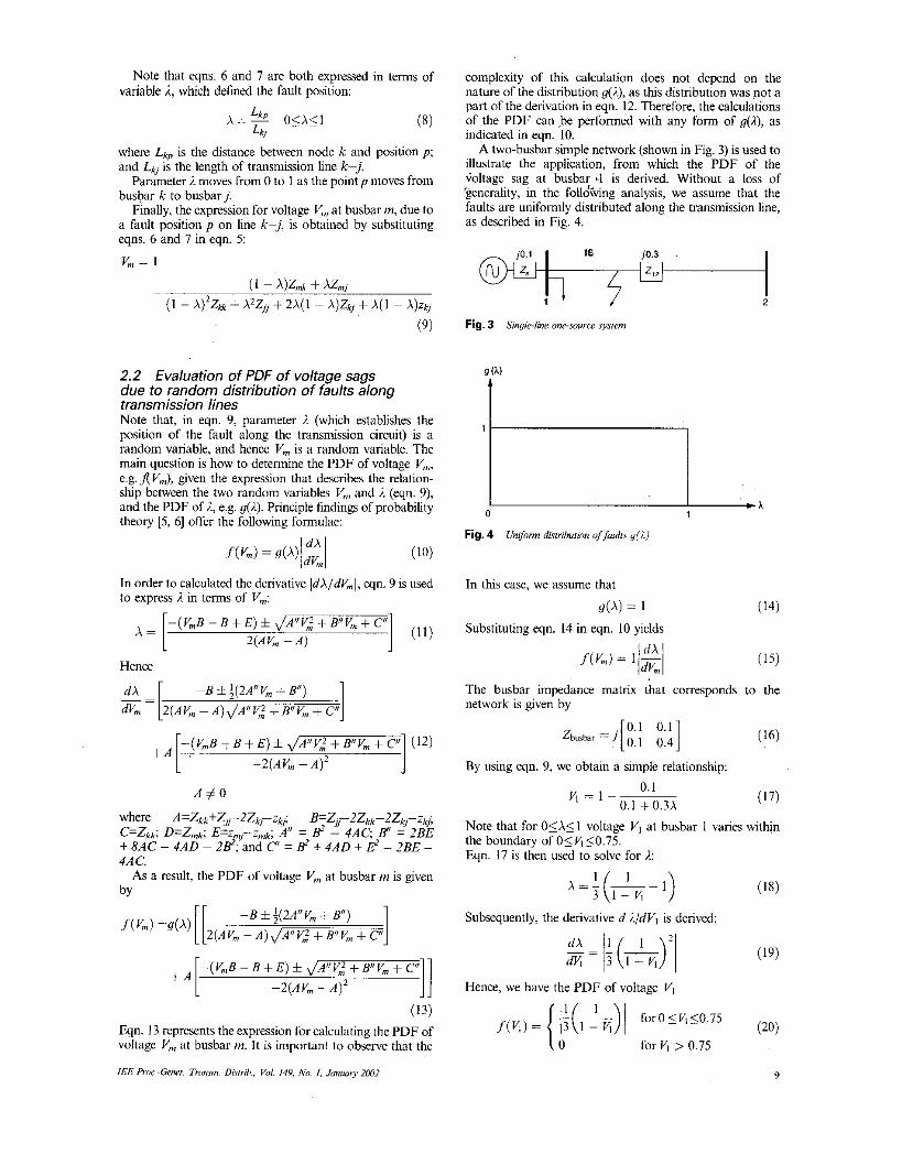
As shown in Fig. S,l(Vl) is depicted by an exponential-like function, with the variable VI lying across a range of a finite interval (O.OO<& 50.75).
0 0.1 0.2 0.3 0.4 0.5 0.6 0.7 0.8 0.9 1.0
voltage magnitude during sags. p.u.
Fig. 5 diwibured foulis along line 1-2 of .sysrem slmiln in Fig. 4
Prohohiliry i1enrir);jUnction of coliagr.~ or hubin- I /or- z~nfbmtly
The standard form of voltage sag presentation is usually in a bar chart, to present the annual number of voltage sags as a function of voltage magnitudes. By knowing the number of faults per year on each transmission line, the PDF representation can be transformed into a standard representation in accordance with the following procedure. Given that
Hence
where a and b are the two ending points of an interval; P(asV1<6) is the probability of a<Vl<b; N(a<&<b) is the number of voltage sags to be observed in the interval a 5 V15b; and N,",, is the total number of faults per year.
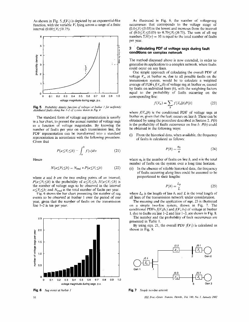
Fig. 6 shows the bar chart presenting the number of sag events to be observed at busbar 1 over the period of one year, given that the number of faults on the transmission line 1-2 is ten per year.
2.5
0 0.1 0.2 0.3 0.4 0.5 0.6 0.7 0.8 0.9 1.0
voltage magnitude during sags. P.U.
Fig. ti Sdg euenrs (11 bushor I
10
As illustrated in Fig. 6, the number of voltage-sag occurrences that corresponds to the voltage range of (O.O<& 50.05) is the lowest and increases from the interval of (O.O<Vl<O.OS) to 0.701Fi10.75). The sum of all sag numbers CN(w) = 10 is equal to the total number of faults per year.
3 Calculating PDF of voltage sags during fault conditions on complex network
The method discussed above is now extended, in order to generalise its application to a complex network, where faults could occur on any lines.
One simple approach of calculating the overall PDF of voltage V,,, at husbar vi, due to all possible faults on the transmission system, would be to calculate a weighted average of PDFsl(V,,,Ib) of voltage sag at husbar m, caused by faults on individual lines (b), with the weighting factors equal to the probability of faults occurring on the corresponding line:
where f(V,,,lh) is the conditional PDF of voltage sags at busbar ni, given that the fault occurs on line b. These can he obtained by using the procedure described in Section 2. P(b) is the probability of faults occurrence on line h. P(b) could be obtained in the following ways:
(i) From the historical data, when available, the frequency of faults is calculated as follows:
where nb is the number of faults on line b_ and n is the total number of faults on the system over a long time horizon. (ii) In the absence of reliable historical data, the frequency
of faults occurring along lines could he assumed to be proportional to their lengths:
Lb P ( 6 ) = ~
L where L,, is the length of line 6, and L is the total length of all lines of the transmission network under consideration.
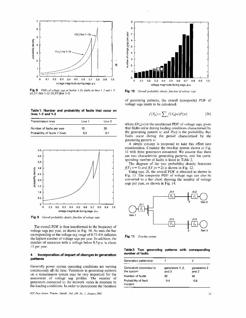
The meaning and the application of eqn. 23 is illustrated on a simple two-line system, shown in Fig. 7. The conditional PDFs,flV,Ib,) andflVllb2) of voltage at busbar I , due to faults on line 1-2 and line 1-3, are shown in Fig. 8.
The number and the probability of fault occurrences are presented in Table I.
By using eqn. 21, the overall PDF,XVl) is calculated as shown in Fig. 9.
( 2 5 )
Gen 1 -1 I
3 Gen 3
7)1111111,,1 6
1
0 0 0.1 0.2 0.3 0.4 0.5 0.6 0.7 0.8 0.9 1.0
voltage magnitude during sags. P.U.
Tablel: Number and probability of faults that occur on lines 1-2 and 1-3
Transmission lines Line 1 Line 2
Number of faults per year 15 35
Probability of faults P (line) 0.3 0.7
01 " " " " ' I 0 0.1 0.2 0.3 0.4 0.5 0.6 0.7 0.8 0.9 1.0
voltage magnitude during sags, p.u.
Fig. 9 & r r d pmhobiliiy deriliryfunciion qf rolioge suqs
The overall PDF is then transformed to the frequency of voltage sags per year, as shown in Fig. IO. As seen the bar corresponding to the voltage sag range of 0.75-0.8 indicates the highest number of voltage sags per year. In addition, the number of occasions with a voltage below 0.5p.u. is about 15 per year.
4 patterns
Generally power system operating conditions are varying continuously all the time. Variations in generating patterns on a transmission system may be very important for the assessment of voltage sag profiles. The number of generators connected to the network varies in response to the loading conditions. In order to incorporate the variation
Incorporation of impact of changes in generation
IEE Proc.-Cenm Trmmn DisirLh.. Vol. 149, No. I , Janmry 2002
0 0.1 0.2 0.3 0.4 0.5 0.6 0.1 0.8 0.9 1.0 voltage magnitude during sags, p.u.
Fig. 10
of generating patterns. the overall (composite) PDF of voltage sags needs to be calculated:
Oacrull prohohilirj doL\irj/ieroion qfwlmge .mgs
whereflV&) is the conditional PDF of voltage sags. given that faults occur during loading conditions characterised by the generating pattern w; and P(w) is the probability that faults occur during the period chdracterised by the generating pattern IC.
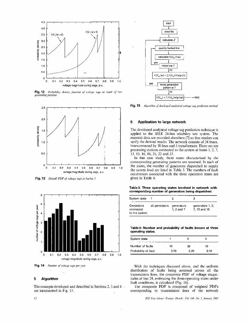
A simple concept is proposed to take this effect into consideration. Consider the two-line system shown in Fig. I I with three generators connected. We assume that there are two characteristic generating patterns? and the corre- sponding number of faults is listed in Table 2.
The diagram of the two probability density functions j(Vlliv= I ) andflViliv=2) is shown in Fig. 12.
Using eqn. 26. the overall PDF is obtained as shown in Fig. 13. The composite PDF of voltage sags can also be converted to a bar chart showing the number of voltage sags per year, as shown in Fig. 14.
j0.3
TableZ: Two generating patterns with corresponding number of faults
Generation patternslw 1 2
Generators connected to generators 1. 2, generators 2 the system and 3 and 3 Number of faults 20 30
Probability of fault 0.4 0.6 incident
I I
3.5
.- 0 3.0 (D
8 2.5 .- 0 2 2.0 - .-
& 1.5
1 .o
0.5
0 ' ' ' I " ' "
I
0 0.1 0.2 0.3 0.4 0.5 0.6 0.7 0.8 0.9 1.0 voltage magnitude during sags, p.u.
Fig. 13 O~wnl i PDF of oo/tage sags or htobol- I
0 0.1 0.2 0.3 0.4 0.5 0.6 0.7 0.8 0.9 1.0 voltage magnitude during sags. P.U.
Fig. 14 h'umhrr ofcolruge sags per y o ,
5 Algorithm
The concepts developed and described in Sections 2 , 3 and 4 are summarised in Fig. 15.
I2
specify faulted line
% more line ? + f(V,iW) = Zf(V,,iIl w ) p (1)
I no I
6 Application to large network
The developed analytical voltage sag prediction technique is applied to the IEEE 24bns reliability test system. The essential data are provided elsewhere [7] so that readers can verify the derived results. The network consists of 24 buses, interconnected by 38 lines and 5 transformers. There are ten generating stations connected to the system at buses 1,2, 7, 13, 15, 16, 18, 21, 22 and 23.
In this case study, three states characterised'by the corresponding generating pattems are assumed, In each of the states, the number of generators dispatched to supply the system load are listed in Table 3. The numbers of fault occurrences associated with the three operation states are given in Table 4.
Table3: Three operating states involved in network with corresponding number of generators being dispatched
System state 1 2 3
Generators all generators generators generators 1, 2. connected 1 , 2 and 7 7, 13 and 15 to the system
Table4 Number and probability of faults known at three operating states
System state 1 2 3
Number of faults 70 20 10
Probability of fault 0.70 0.20 0.10
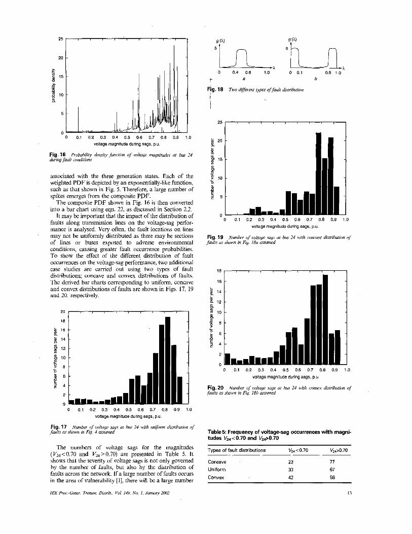
With the techniques discussed above. and the uniform distribution of faults being assumed across all the transmission lines, the composite PDF of voltage magni- tudes at bus 24; embracing the three-operating states under fault conditions, is calculated (Fig. 16).
The composite PDF is composed of weighted PDFs corresponding to transmission lines of the network
IEE Pm.-Gcncr. Tronni Dimih.. V d 149. No. 1. f m u m y 2002
I 20
0 0.4 0.6 1.0 0 0.1 0.9 1.0 a b t
Fig. 18 Two d$ierrent types offault diwiburion ,
0 0.1 0.2 0.3 0.4 0.5 0.6 0.7 0.8 0.9 1.0 voltage magnitude during sags. p.u.
Fig. 16 Probabiliry demirfy ~Iutction of mlfage magnitudes ot h r r 24 &&g fault euditionr
associated with the three generation states. Each of the weighted PDF is depicted by an exponentially-like function, such as that shown in Fig. 5. Therefore, a large number of spikes emerges from the composite PDF.
The composite PDF shown in Fig. 16 is then converted into a bar chart using eqn. 22, as discussed in Section 2.2.
It may be important that the impact of the distribution of faults along transmission lines on the voltage-sag perfor- mance is analysed. Very -often, the fault locations on lines may not be uniformly distributed as there may be sections of lines or buses exposed to adverse environmental conditions, causing greater fault occurrence probabilities. To show the effect of the different distribution of fault occurrences on the voltage-sag performance, two additional case studies are camed out using two types of fault distributions; concave and convex distributions of faults. The derived bar charts corresponding to uniform, concave and convex distributions of faults are shown in Figs. 17, 19 and 20, respectively.
2 0 1 , , , I , , I , I ,
5 20 5.
a YI
b
p 15 m - B
: 5
4 10 - m P
0 0 0.1 0.2 0.3 0.4 0.5 0.6 0.7 0.8 0.9 1.0
voltage magnitude during sags, p.u
Fig. 19 faults m shown in Fig. I& m m d
Number of uoltuge sags of bur 24 with concove disrriburion sf
1 6 , , , , , . I , I I I
0 0.1 0.2 0.3 0.4 0.5 0.6 0.7 0.8 0.9 1.0 voltage magnitude during sags, p.u.
Fig. 17 Jdts ui shown in Fig. 4
Number o/ .oltage sags or bur 24 with mifDnn didburion o/
The numbers of voltage sags for the magnitudes (V*4<0.70 and V24>0.70) are presented in Table 5. It shows that the seventy of voltage sags is not only governed by the number of faults, but also by the distribution of faults across the network. If a large number of faults occurs in the area of vulnerability [I], there will be a large number
IEE Proc.-Gener. Tro" Diwib.. Yo1 I49, No. 1. J m w ~ r y 2002
0 0.1 0.2 0.3 0.4 0.5 0.6 0.7 0.6 0.9 1.0 voltage magnitude during sags, P.U.
Fig. 20 Numher of aoltaye sags at bur 24 with conwr dirtributim of fnult. m Jhow in Fig. 186 assumed
Table5 Frequency of voltage-sag Occurrences with magni- tudes V2.,<0.70 and V2p0.70
~~ ~~ ~~
Types of fault distributions V?n<0.70 Vz4>O.70
Concave
Uniform
Convex
23 77
33 67
42 58
13
of voltage sags with greater severity at a bus of concern. For example, the number of sags with magnitudes less than 0.70p.u. is the highest for the convex distributions of fault, and vice oersu for the concave distribution of faults. This'is because the convex distribution causes a greater number of faults being distributed on the area of vulnerability, hence increasing the frequency of Severe voltage sags to be observed at bus 24.
7 Conclusions
An analytical method based on the concept of fault position has been presented for quantifying voltage sags at a bus of interest by the means of probability density function. The Z-bus matrix, used to deal with fault positions by calculating the corresponding transfer and driving impe- dances, has^ been used here to derive the analytical expression of voltage sag distributions. The technique has been further extended to deal with the randomness of fault locations on the transmission circuits, as well as the variations in generating patterns. The validity and potential usage of the approach are demonstrated on the IEEE 24 bus reliability test system. Work associated with the incorporation of various types of unbalanced faults and the topology changes of the network would be carried out in the near future to extend the applicability of the method.
8 Acknowledgments
The authors gratefully acknowledge the research grants given by EPSRC under grant GM/M03405 and ORs.
9
I
2
3
4
5
6
7
n
9
10
References
DUGAN, R.C., MCGRANAGHAN, M.F., and BEATY, H.W.: 'Electrical powm systems quality'. Is1 Fdn. (McGraw-Hill, I""', I,,",
BOLLEN, M.H.J.: 'Undcrstandng pawr qualify p m b l m : voltage s m and interruptions'. 1st Edn. (IEEE P m Series On Power Engineering IEEE, Ncw York, 2000) HAN, Z.X.: 'Generalised mcthcd of analysis of simultaneous fault! in elcdric cower svstem'. IEEE Trams. Power Annor. Sw.. 1982. PAS . . ~ ~, , . 101, (lfl), pp. 363r3942 GRAINGER J . J . , and STEVENSON. W.D.: 'Power system analysis'. 4th Edn. (McGraw-Hill Intcmational, 1982) WALPOLE. R.E., and MYERS, R.H.: 'ProbabiPty and statistics for engineers and scientists'. 5th Edn. (Prenticc Hall, Englewaad Cliffs. New Jersey, USA, 1993) ANDERS. GJ.: 'Probability concepts in eloctcc p w c r system' (John Wilev & Sons. 1989) , ~~ ~~
IEEE Reliability Tkt System, IEEE Trms. Pow? Appm. Syxr.. 1979, PAS-98, (61, pp. 2047-2054 BOLLEN. M.H.J., QADER. M.R., and ALLAN. R.N.: 'Stochastic pmdiction of vollagc sags in the reliability test system.' FQA-97 June 1997 Eurone. 1Elfonk~ Sweden) ,. . ~ ~ ~ ~ , QADER. M.R:A.: 'Stochastic asscssmenf of voltagc ags due lo shon circuit in cktrical networks: PhD t h i s , UMIST, UK. 1997 EL-KADY, M.A.: 'Probabilistic shonsircuit analysis by Monte-Carlo simulations', IEEE Trow. Pou,er Apprrr. Sysr.. 1983, PAS-102, (S ) , pp. 1308-1316
14


