
Applied Math for Engineers
Ming Zhong
Lecture 13
March 12, 2018
Ming Zhong (JHU) AMS Spring 2018 1 / 24

Linear Algebra
Table of Contents
1 Linear Algebra
2 Differential Vector Calculus
3 Integral Vector Calculus
4 First Order ODEs
5 Second Order ODEs
6 High Order ODEs
7 First Order ODE Systems
Ming Zhong (JHU) AMS Spring 2018 2 / 24
Linear Algebra
Summary
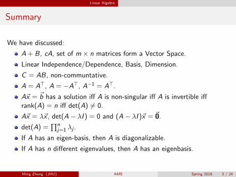
We have discussed:
A + B, cA, set of m × n matrices form a Vector Space.
Linear Independence/Dependence, Basis, Dimension.
C = AB, non-communtative.
A = A>, A = −A>, A−1 = A>.
A~x = ~b has a solution iff A is non-singular iff A is invertible iffrank(A) = n iff det(A) 6= 0.
A~x = λ~x , det(A− λI ) = 0 and (A− λI )~x = ~0.
det(A) =∏n
j=1 λj .
If A has an eigen-basis, then A is diagonalizable.
If A has n different eigenvalues, then A has an eigenbasis.
Ming Zhong (JHU) AMS Spring 2018 3 / 24

Linear Algebra
Example
Example
Transform, 9x21 − 6x1x2 + 17x2
2 = 26, to the canonical form (to principal
axes). Express
[x1
x2
]in terms of the new variables
[y1
y2
].
A =
[9 −3−3 17
].
det(A− λI ) = λ2 − 26λ+ 144 = (x − 8)(x − 18).
λ = 8, A− 8I =
[1 −3−3 9
], ~x1 =
[3√101√10
].
λ = 18, A− 18I =
[−9 −3−3 −1
], ~x1 =
[1√10−3√
10
].
Ming Zhong (JHU) AMS Spring 2018 4 / 24

Linear Algebra
Example, Cont.
Example
Originally, we have B = ~x>A~x − 36 = 0
P =
[3√10
1√10
1√10
−3√10
], P−1 = P>.
A = PDP−1 = PDP>, so ~x>PDP>~x = (P>~x)>D(P>~x).
~y = P>~x , so ~x = P~y .
B = λ1y21 + λ2y
22 − 36 = 8y2
1 + 18y22 − 36 = 0.
Ming Zhong (JHU) AMS Spring 2018 5 / 24
Differential Vector Calculus
Table of Contents
1 Linear Algebra
2 Differential Vector Calculus
3 Integral Vector Calculus
4 First Order ODEs
5 Second Order ODEs
6 High Order ODEs
7 First Order ODE Systems
Ming Zhong (JHU) AMS Spring 2018 6 / 24

Differential Vector Calculus
Summary
We have discussed:
~a · ~b =∣∣∣∣~a∣∣∣∣ · ∣∣∣∣~b∣∣∣∣ cos(γ),
∣∣∣∣~a× ~b∣∣∣∣ =
∣∣∣∣~a∣∣∣∣ · ∣∣∣∣~b∣∣∣∣ sin(γ).
~a · (~b × ~c) = (~a× ~b) · ~c , and∣∣~a · (~b × ~c)
∣∣.Given f (x , y , z), grad(f ) = ∇f =
∂f∂x∂f∂y∂f∂z
.
D~uf = ~u · grad(f ), only when ~u is a unit vector.
div(~f ) = ∇ · ~f = ∂f1∂x + ∂f2
∂y + ∂f3∂z .
curl(~f ) = ∇× ~f .
curl(grad(f )) = ~0 and div(curl(~f )) = 0.
Ming Zhong (JHU) AMS Spring 2018 7 / 24

Differential Vector Calculus
Eample
Show that div(curl(~f )) = 0.
div(curl(~f )) = ∇ · curl(~f ) = ∇ · (∇× ~f ) = (∇×∇) · ~f = 0.
Ming Zhong (JHU) AMS Spring 2018 8 / 24
Integral Vector Calculus
Table of Contents
1 Linear Algebra
2 Differential Vector Calculus
3 Integral Vector Calculus
4 First Order ODEs
5 Second Order ODEs
6 High Order ODEs
7 First Order ODE Systems
Ming Zhong (JHU) AMS Spring 2018 9 / 24

Integral Vector Calculus
Summary
We have discussed:∫C~f (~r) · d~r =
∫ ba~f (~r(t)) · d~r
dt dt.
~f is path independence if ~f = grad(f ).
Green’s theorem:∫∫
R(∂f2∂x −∂f1∂y ) dA =
∮C~f (~r) · d~r , R is a closed and
simply connected Region, and C is its boundary.∫∫S~f (~r)· d ~S =
∫∫R~f (~r(u, v)) · (~ru × ~rv )dA (check orientation).
Divergence theorem of Gauss:∫∫∫
V div(~f ) dV =∫∫
S~f (~r) · d ~S (the
surface normal ~n is pointing out and V is an enclosed region, S is itsboundary surface).
Stokes’s theorem:∫∫
S curl(~f (~r)) · d ~S =∮C~f (~r) · d~r (S is simply
connected).
Ming Zhong (JHU) AMS Spring 2018 10 / 24

Integral Vector Calculus
Example
Example
Evaluate the integral,∫∫
S~f (~r) · d ~S , directly or if possible by the divergence
theorem. Show details:
~f =
111
, S : x2 + y2 + 4z2 = 4, z ≥ 0.
S does not enclose any area, so no divergence.
S : x2 + y2 + 4z2 = 4⇒ f (x , y) =√
1− x2
4 −y2
4 , Domain:
R : x2 + y2 ≤ 4.
~r(x , y) =
xy√
1− x2
4 −y2
4
.
Ming Zhong (JHU) AMS Spring 2018 11 / 24

Integral Vector Calculus
Example, Cont.
Example
~rx =
10−x4√
1− x2
4− y2
4
and ~ry =
01−y
4√1− x2
4− y2
4
.
~rx × ~ry =x4√
1− x2
4− y2
4
~i +y4√
1− x2
4− y2
4
~j + ~k = −fx~i +−fy~j + ~k.
~f · (~rx × ~ry ) =x+y
4√1− x2
4− y2
4
+ 1.
Use Polar: x = r cos(θ) and y = r sin(θ), 0 ≤ r ≤ 2 and 0 ≤ θ ≤ 2π.
Any other way?
Ming Zhong (JHU) AMS Spring 2018 12 / 24

First Order ODEs
Table of Contents
1 Linear Algebra
2 Differential Vector Calculus
3 Integral Vector Calculus
4 First Order ODEs
5 Second Order ODEs
6 High Order ODEs
7 First Order ODE Systems
Ming Zhong (JHU) AMS Spring 2018 13 / 24

First Order ODEs
Summary
We have discussed:
F (x , y , y ′) = 0 (implicit form) and y ′ = f (x , y) (explicit form).
Separable ODEs: g(y)dy = h(x)dx , integrate, G (y) = H(x) + C .
y ′ = f (x , y) = f ( yx ), let u = yx .
Exact ODEs: M(x , y)dx + N(x , y)dy = 0 when ∂M∂y = ∂N
∂x .
Integrate M w.r.t. x , obtain u(x , y), then differentiate u w.r.t. y .
P(x , y)dx + Q(x , y)dy is not exact, then use integrating factor.
Linear ODEs: y ′+ p(x)y = r(x), integrating factor: F (x) = e∫p(x) dx .
Bernoulli ODEs: y ′ + p(x)y = g(x)yα, when α 6= 0 and αneq1, thenu = y1−α.
Ming Zhong (JHU) AMS Spring 2018 14 / 24
First Order ODEs
Example
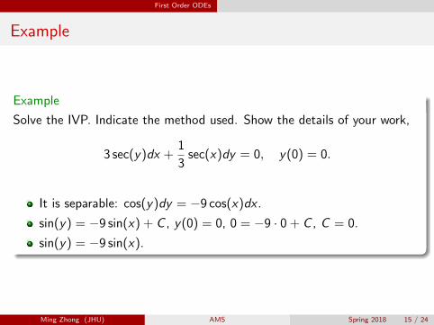
Example
Solve the IVP. Indicate the method used. Show the details of your work,
3 sec(y)dx +1
3sec(x)dy = 0, y(0) = 0.
It is separable: cos(y)dy = −9 cos(x)dx .
sin(y) = −9 sin(x) + C , y(0) = 0, 0 = −9 · 0 + C , C = 0.
sin(y) = −9 sin(x).
Ming Zhong (JHU) AMS Spring 2018 15 / 24

Second Order ODEs
Table of Contents
1 Linear Algebra
2 Differential Vector Calculus
3 Integral Vector Calculus
4 First Order ODEs
5 Second Order ODEs
6 High Order ODEs
7 First Order ODE Systems
Ming Zhong (JHU) AMS Spring 2018 16 / 24
Second Order ODEs
Summary
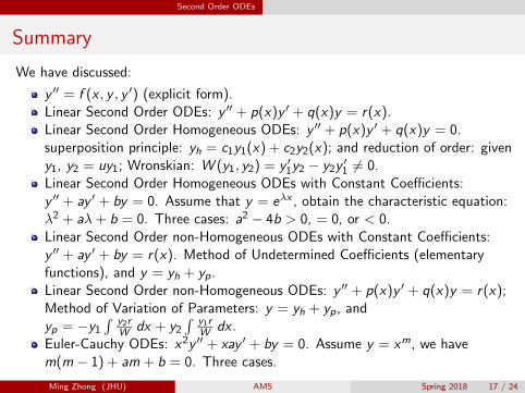
We have discussed:
y ′′ = f (x , y , y ′) (explicit form).Linear Second Order ODEs: y ′′ + p(x)y ′ + q(x)y = r(x).Linear Second Order Homogeneous ODEs: y ′′ + p(x)y ′ + q(x)y = 0.superposition principle: yh = c1y1(x) + c2y2(x); and reduction of order: giveny1, y2 = uy1; Wronskian: W (y1, y2) = y ′1y2 − y2y
′1 6= 0.
Linear Second Order Homogeneous ODEs with Constant Coefficients:y ′′ + ay ′ + by = 0. Assume that y = eλx , obtain the characteristic equation:λ2 + aλ+ b = 0. Three cases: a2 − 4b > 0, = 0, or < 0.Linear Second Order non-Homogeneous ODEs with Constant Coefficients:y ′′ + ay ′ + by = r(x). Method of Undetermined Coefficients (elementaryfunctions), and y = yh + yp.Linear Second Order non-Homogeneous ODEs: y ′′ + p(x)y ′ + q(x)y = r(x);Method of Variation of Parameters: y = yh + yp, andyp = −y1
∫ y2rW dx + y2
∫ y1rW dx .
Euler-Cauchy ODEs: x2y ′′ + xay ′ + by = 0. Assume y = xm, we havem(m − 1) + am + b = 0. Three cases.
Ming Zhong (JHU) AMS Spring 2018 17 / 24

Second Order ODEs
Example
Example
Find a general solution. Show the details of your calculation.
y ′′ + 16y = 17ex , y(0) = 6, y ′(0) = −2.
y ′′ + 16y = 10, λ2 + 16λ = 0, λ1 = 0, and λ2 = −16.
yh = c1 + c2e−16x .
yp = Kex , y ′p = Kex , y ′′ = Kex , Kex + 16Kex = 16ex , K = 1.
y = c1 + c2e−16x + ex , y(0) = c1 + c2 + 1 = 6,
y ′(0) = −16c2 + 1 = −2.
c2 = 316 and c1 = 5− 3
16 .
Ming Zhong (JHU) AMS Spring 2018 18 / 24

High Order ODEs
Table of Contents
1 Linear Algebra
2 Differential Vector Calculus
3 Integral Vector Calculus
4 First Order ODEs
5 Second Order ODEs
6 High Order ODEs
7 First Order ODE Systems
Ming Zhong (JHU) AMS Spring 2018 19 / 24
High Order ODEs
Summary
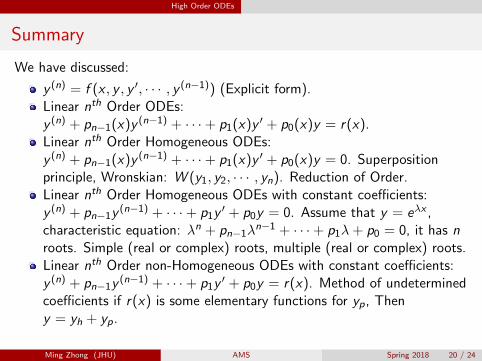
We have discussed:
y (n) = f (x , y , y ′, · · · , y (n−1)) (Explicit form).Linear nth Order ODEs:y (n) + pn−1(x)y (n−1) + · · ·+ p1(x)y ′ + p0(x)y = r(x).Linear nth Order Homogeneous ODEs:y (n) + pn−1(x)y (n−1) + · · ·+ p1(x)y ′ + p0(x)y = 0. Superpositionprinciple, Wronskian: W (y1, y2, · · · , yn). Reduction of Order.Linear nth Order Homogeneous ODEs with constant coefficients:y (n) + pn−1y
(n−1) + · · ·+ p1y′ + p0y = 0. Assume that y = eλx ,
characteristic equation: λn + pn−1λn−1 + · · ·+ p1λ+ p0 = 0, it has n
roots. Simple (real or complex) roots, multiple (real or complex) roots.Linear nth Order non-Homogeneous ODEs with constant coefficients:y (n) + pn−1y
(n−1) + · · ·+ p1y′ + p0y = r(x). Method of undetermined
coefficients if r(x) is some elementary functions for yp, Theny = yh + yp.
Ming Zhong (JHU) AMS Spring 2018 20 / 24

High Order ODEs
Example
Linear nth Order non-Homogeneous ODEs:y (n) + pn−1(x)y (n−1) + · · ·+ p1(x)y ′ + p0(x)y = r(x). Method of
variation of parameters. yp =∑n
j=1 yj(x)∫ Wj (x)
W (x) r(x) dx . Wj is obtained
by replacing the j th column of W by[0, · · · , 0, 1
]>.
Example
Solve the given ODE. Show the details of your work,
y ′′′ + 4y ′′ + 13y ′ = 0.
λ3 + 4λ2 + 13λ = 0, λ(λ2 + 4λ+ 13) = 0.λ1 = 0, ∆ = 16− 52 = −36 = (6i)2 < 0.λ2,3 = −4±6i
2 = −2± 3i .yh = c1 + e−2x(c2 cos(3x) + c3 sin(3x)).
Ming Zhong (JHU) AMS Spring 2018 21 / 24

First Order ODE Systems
Table of Contents
1 Linear Algebra
2 Differential Vector Calculus
3 Integral Vector Calculus
4 First Order ODEs
5 Second Order ODEs
6 High Order ODEs
7 First Order ODE Systems
Ming Zhong (JHU) AMS Spring 2018 22 / 24

First Order ODE Systems
Summary
We have discussed:
~y ′ = ~f (t, ~y) (Explicit form). Caution: t or x , it does not really matter.
Linear Systems of ODEs: ~y ′ = A(t)~y + ~g(t), where A is a matrix.
Linear Homogeneous Systems of ODEs: ~y ′ = A(t)~y . Superpositionprinciple. Fundamental matrix Y =
[~y1, · · · , ~yn
], Wronskian,
W (~y1, · · · , ~yn) = det([~y1, · · · , ~yn
]) = det(Y ), ~yj ’s are the basis
solutions.
Linear Homogeneous Systems of ODEs with constant coefficients:~y ′ = A~y . A has an eigen-basis, ~xj ’s are n linearly independenteigen-vectors of A, then ~yj = ~xje
λjx .
Categorizing the critical point yc =
[00
]. We consider λ1 + λ2, λ1λ2
and (λ1 − λ2)2.
Ming Zhong (JHU) AMS Spring 2018 23 / 24

First Order ODE Systems
Example
Find a general solution. Determine the kind and stability of the criticalpoint.
y ′1 = 3y1 + 4y2
y ′2 = 3y1 + 2y2
A =
[3 43 2
], det(A− λI ) = λ2 + 5λ− 6 = 0.
λ1 = −6 and λ2 = 1.
~x1 =
[43
]and ~x2 =
[1−1
].
~yh = c1~x1e−6t + c2~x2e
t .
p = λ1 + λ2 = −5 < 0, q = λ1λ2 = −6 < 0,∆ = (λ1 − λ2)2 = 49 > 0, real, opposite signs, Saddle point.
Ming Zhong (JHU) AMS Spring 2018 24 / 24

![[Algebra a] Fundamentos de Algebra](https://cdn.vdocuments.net/doc/165x107/55cf9bca550346d033a76685/algebra-a-fundamentos-de-algebra.jpg)


