Download - Assessment for Decision-Makers
Assessment for Decision-Makers
WMO Global Ozone Research andMonitoring Project – Report No. 56
Scienti�c Assessment of Ozone Depletion: 2014
World Meteorological OrganizationUnited Nations Environment Programme
National Oceanic and Atmospheric AdministrationNational Aeronautics and Space Administration
European Commission
World Meteorological Organization7bis, avenue de la PaixCase postale 2300CH-1211, Geneva 2Switzerland
United Nations Environment ProgrammeOzone SecretariatP.O. Box 30552Nairobi, 00100Kenya
U.S. Department of CommerceNational Oceanic and Atmospheric Administration14th Street and Constitution Avenue NWHerbert C. Hoover Building, Room 5128Washington, D.C. 20230
National Aeronautics and Space AdministrationEarth Science DivisionNASA Headquarters300 E Street SWWashington, D.C. 20546-0001
European CommissionDirectorate-General for Research and InnovationB-1049 BruxellesBelgium
Published online September 2014Published in print December 2014
ISBN: 978-9966-076-00-7
Hardcopies of this report are available from WMO (address above; [email protected]).
This report and other components of the 2014 Ozone Assessment are available at the following locations:http://www.wmo.int/pages/prog/arep/gaw/ozone_2014/ozone_asst_report.htmlhttp://ozone.unep.org/en/assessment_panels_bodies.php?committee_id=7http://ozone.unep.org/Assessment_Panels/SAP/SAP2014_Assessment_for_Decision-Makers.pdfhttp://esrl.noaa.gov/csd/assessments/ozone/
Note: Figures from this report are in the public domain and may be used with proper attribution to source.
This document should be cited as:WMO (World Meteorological Organization), Assessment for Decision-Makers: Scientific Assessment of Ozone Depletion: 2014, 88 pp., Global Ozone Research and Monitoring Project—Report No. 56, Geneva, Switzerland, 2014.
Cover design: Christine A. Ennis, Debra A. Dailey-Fisher, and Albert Romero Cover photo adapted from: ©iStock.com/sharply_done
World Meteorological OrganizationGlobal Ozone Research and Monitoring Project—Report No. 56
National Oceanic and Atmospheric AdministrationNational Aeronautics and Space Administration
United Nations Environment ProgrammeWorld Meteorological Organization
European Commission
Assessment for Decision-MakersScientific Assessment of Ozone Depletion: 2014

ES-1
Actions taken under the Montreal Protocol have led to decreases in the atmospheric abundance of controlled ozone-depleting substances (ODSs), and are enabling the return of the ozone layer toward 1980 levels.
• The sum of the measured tropospheric abundances of substances controlled under the Montreal Protocol continues to decrease. Most of the major controlled ODSs are decreasing largely as projected, and hydrochlorofluorocarbons (HCFCs) and halon-1301 are still increasing. Unknown or unreported sources of carbon tetrachloride are needed to explain its abundance.
• Measured stratospheric abundances of chlorine- and bromine-containing substances originating from the degradation of ODSs are decreasing. By 2012, combined chlorine and bromine levels (as estimated by Equivalent Effective Stratospheric Chlorine, EESC) had declined by about 10–15% from the peak values of ten to fifteen years ago. Decreases in atmospheric abundances of methyl chloroform (CH3CCl3), methyl bromide (CH3Br), and chlorofluorocarbons (CFCs) contributed approximately equally to these reductions.
• Total column ozone declined over most of the globe during the 1980s and early 1990s (by about 2.5% averaged over 60°S to 60°N). It has remained relatively unchanged since 2000, with indications of a small increase in total column ozone in recent years, as expected. In the upper stratosphere there is a clear recent ozone increase, which climate models suggest can be explained by comparable contributions from declining ODS abundances and upper stratospheric cooling caused by carbon dioxide increases.
• The Antarctic ozone hole continues to occur each spring, as expected for the current ODS abundances. The Arctic stratosphere in winter/spring 2011 was particularly cold, which led to large ozone depletion as expected under these conditions.
• Total column ozone will recover toward the 1980 benchmark levels over most of the globe under full compliance with the Montreal Protocol. This recovery is expected to occur before midcentury in midlatitudes and the Arctic, and somewhat later for the Antarctic ozone hole.
The Antarctic ozone hole has caused significant changes in Southern Hemisphere surface climate in the summer.
• Antarctic lower stratospheric cooling due to ozone depletion is very likely the dominant cause of observed changes in Southern Hemisphere tropospheric summertime circulation over recent decades, with associated impacts on surface temperature, precipitation, and the oceans. In the Northern Hemisphere, no robust link has been found between stratospheric ozone depletion and tropospheric climate.
Changes in CO2 , N2O, and CH4 will have an increasing influence on the ozone layer as ODSs decline.
• As controlled ozone-depleting substances decline, the evolution of the ozone layer in the second half of the 21st century will largely depend on the atmospheric abundances of CO2, N2O, and CH4. Overall, increasing carbon dioxide (CO2 ) and methane (CH4 ) elevate global ozone, while increasing nitrous oxide (N2O) further depletes global ozone. The Antarctic ozone hole is less sensitive to CO2, N2O, and CH4 abundances.
• In the tropics, significant decreases in column ozone are projected during the 21st century. Tropical ozone levels are only weakly affected by ODS decline; they are sensitive to circulation changes driven by CO2 , N2O, and CH4 increases.
The climate benefits of the Montreal Protocol could be significantly offset by projected emissions of HFCs used to replace ODSs.
The Montreal Protocol and its Amendments and adjustments have made large contributions toward reducing global greenhouse gas emissions. In 2010, the decrease of annual ODS emissions under the Montreal Protocol is estimated to be about 10 gigatonnes of avoided CO2-equivalent emissions per year, which is about five times larger than the annual emissions reduction target for the first commitment period (2008–2012) of the Kyoto Protocol (from the Executive Summary of the Scientific Assessment of Ozone Depletion: 2010).1
1 GWP-weighted emissions, also known as CO2-equivalent emissions, are defined as the amount of gas emitted multiplied by its 100-year Global Warming Potential (GWP). Part of the effect of ODSs as greenhouse gases is offset by the cooling due to changes in ozone.
Executive Summary
ES-2
• The sum of the hydrofluorocarbons (HFCs) currently used as ODS replacements makes a small contribution of about 0.5 gigatonnes CO2-equivalent emissions per year. These emissions are currently growing at a rate of about 7% per year and are projected to continue to grow.
• If the current mix of these substances is unchanged, increasing demand could result in HFC emissions of up to 8.8 gigatonnes CO2-equivalent per year by 2050, nearly as high as the peak emission of CFCs of about 9.5 gigatonnes CO2-equivalent per year in the late 1980s.2
• Replacements of the current mix of high-Global Warming Potential (GWP) HFCs with low-GWP compounds or not-in-kind technologies would essentially avoid these CO2-equivalent emissions.
• Some of these candidate low-GWP compounds are hydrofluoro-olefins (HFOs), one of which (HFO-1234yf ) yields the persistent degradation product trifluoroacetic acid (TFA) upon atmospheric oxidation. While the environmental effects of TFA are considered to be negligible over the next few decades, potential longer-term impacts could require future evaluations due to the environmental persistence of TFA and uncertainty in future uses of HFOs.
• By 2050, HFC banks are estimated to grow to as much as 65 gigatonnes CO2-equivalent. The climate change impact of the HFC banks could be reduced by limiting future use of high-GWP HFCs to avoid the accumulation of the bank, or by destruction of the banks.
Additional important issues relevant to the Parties to the Montreal Protocol and other decision-makers have been assessed.
• Derived emissions of carbon tetrachloride (CCl4), based on its estimated lifetime and its accurately measured atmospheric abundances, have become much larger than those from reported production and usage over the last decade.
• As of 2009, the controlled consumption of methyl bromide declined below the reported consumption for quarantine and pre-shipment (QPS) uses, which are not controlled by the Montreal Protocol.
• Increased anthropogenic emissions of very short-lived substances (VSLS) containing chlorine and bromine, particularly from tropical sources, are an emerging issue for stratospheric ozone. The relative contribution of these emissions could become important as levels of ODSs controlled under the Montreal Protocol decline.
• As the atmospheric abundances of ODSs continue to decrease over the coming decades, N2O, as the primary source of nitrogen oxides in the stratosphere, will become more important in future ozone depletion.
• Emissions of HFC-23, a by-product of HCFC-22 production, have continued despite mitigation efforts.
• While ODS levels remain high, a large stratospheric sulfuric aerosol enhancement due to a major volcanic eruption or geoengineering activities would result in a substantial chemical depletion of ozone over much of the globe.
While past actions taken under the Montreal Protocol have substantially reduced ODS production andconsumption, additional, but limited, options are available to reduce future ozone depletion.
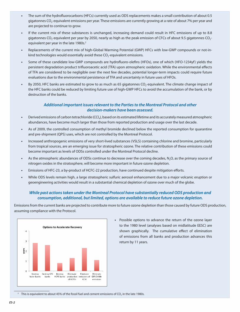
Emissions from the current banks are projected to contribute more to future ozone depletion than those caused by future ODS production, assuming compliance with the Protocol.
• Possible options to advance the return of the ozone layer to the 1980 level (analyses based on midlatitude EESC) are shown graphically. The cumulative effect of elimination of emissions from all banks and production advances this return by 11 years.
2 This is equivalent to about 45% of the fossil fuel and cement emissions of CO2 in the late 1980s.
i
The present document will be part of the information upon which the Parties to the United Nations Montreal Protocol will base their future decisions regarding ozone-depleting substances, their alternatives, and protection of the ozone layer. It is the latest in a long series of scientific assessments that have informed the Parties.
The Charge to the Assessment PanelsSpecifically, the Montreal Protocol on Substances that Deplete the Ozone Layer 3 states (Article 6): “…the Parties shall assess the control measures…on the basis of available scientific, environmental, technical, and economic information. ” To provide the mechanisms whereby these assessments are conducted, the Protocol further states: “…the Parties shall convene appropriate panels of experts” and “the panels will report their conclusions…to the Parties.”
To meet this request, the Scientific Assessment Panel (SAP), the Environmental Effects Assessment Panel (EEAP), and the Technology and Economic Assessment Panel (TEAP) have each prepared, about every 3–4 years, major assessment reports that updated the state of understanding in their purviews. These reports have been scheduled so as to be available to the Parties in advance of their meetings at which they consider the need to amend or adjust the Protocol.
The Sequence of Scientific AssessmentsThe present 2014 report is the latest in a series of twelve scientific Assessments (shown below) prepared by the world’s leading experts in the atmospheric sciences and under the international auspices of the World Meteorological Organization (WMO) and/or the United Nations Environment Programme (UNEP). This report is the eighth in the set of major Assessments that have been prepared by the Scientific Assessment Panel directly as input to the Montreal Protocol process. The chronology of all the scientific Assessments on the understanding of ozone depletion and their relation to the international policy process is summarized as follows:
Year Policy Process Scientific Assessment
1981 The Stratosphere 1981: Theory and Measurements. WMO No. 11
1985 Vienna Convention Atmospheric Ozone 1985. Three volumes. WMO No. 16
1987 Montreal Protocol
1988 International Ozone Trends Panel Report 1988. Two volumes. WMO No. 18
1989 Scientific Assessment of Stratospheric Ozone: 1989. Two volumes. WMO No. 20
1990 London Amendment and adjustments
1991 Scientific Assessment of Ozone Depletion: 1991. WMO No. 25
1992 Methyl Bromide: Its Atmospheric Science, Technology, and Economics (Assessment Supplement). UNEP (1992).
1992 Copenhagen Amendment and adjustments
1994 Scientific Assessment of Ozone Depletion: 1994. WMO No. 37
1995 Vienna adjustments
1997 Montreal Amendment and adjustments
1998 Scientific Assessment of Ozone Depletion: 1998. WMO No. 44
1999 Beijing Amendment and adjustments
2002 Scientific Assessment of Ozone Depletion: 2002. WMO No. 47
2006 Scientific Assessment of Ozone Depletion: 2006. WMO No. 50
2007 Montreal adjustments
2010 Scientific Assessment of Ozone Depletion: 2010. WMO No. 52
2014 Scientific Assessment of Ozone Depletion: 2014. WMO No. 55
Preface
3 In this report, ozone-depleting substances (ODSs) refer to the gases listed in the Annexes to the Montreal Protocol. In addition to these gases, other chemicals also influence the ozone layer, and they are referred to as ozone-relevant gases.
ii
The Current Information Needs of the PartiesThe genesis of Scientific Assessment of Ozone Depletion: 2014 was the 23rd Meeting of the Parties to the Montreal Protocol held during 21–25 November 2011 in Bali, Indonesia, at which the scope of the scientific needs of the Parties was defined in their Decision XXIII/13 (4), which stated that “...for the 2014 report, the Scientific Assessment Panel should consider issues including:
• Assessment of the state of the ozone layer and its future evolution, including in respect of atmospheric changes from, for example, sudden stratospheric warming or accelerated Brewer-Dobson circulation;
• Evaluation of the Antarctic ozone hole and Arctic winter/spring ozone depletion and the predicted changes in these phenomena, with a particular focus on temperatures in the polar stratosphere;
• Evaluation of trends in the concentration in the atmosphere of ozone-depleting substances and their consistency with reported production and consumption of those substances and the likely implications for the state of the ozone layer and the atmosphere;
• Assessment of the interaction between the ozone layer and the atmosphere; including: (i) The effect of polar ozone depletion on tropospheric climate and (ii) The effects of atmosphere-ocean coupling;
• Description and interpretation of observed ozone changes and ultraviolet radiation, along with future projections and scenarios for those variables, taking into account among other things the expected impacts to the atmosphere;
• Assessment of the effects of ozone-depleting substances and other ozone-relevant substances, if any, with stratospheric influences, and their degradation products, the identification of such substances, their ozone-depletion potential and other properties;
• Identification of any other threats to the ozone layer.”
The 2014 SAP Assessment has addressed all the issues that were feasible to address to the best possible extent. Further, given the change in the structure of the report and the evolution of science, the UV changes will be addressed by the Environmental Effects Assessment Panel (EEAP) of the Montreal Protocol. The SAP has provided the necessary information on ozone levels, now and in the future, to EEAP as input to their assessments.
The 2014 Assessment ProcessThe formal planning of the current Assessment was started early in 2013. The Cochairs considered suggestions from the Parties regarding experts from their countries who could participate in the process. Two key changes were incorporated for the 2014 Assessment: (1) creation of a Scientific Steering Committee consisting of the Cochairs and four other prominent scientists; and (2) instituting Chapter Editors for each chapter to ensure that the reviews were adequately and appropriately handled by the authors and key messages were clearly enunciated to take them to the next level. For this reason, the Chapter Editors are also Coauthors of the Assessment for Decision Makers (ADM) of the Scientific Assessment of Ozone Depletion: 2014. The plan for this Assessment was vetted by an ad hoc international scientific advisory group. This group also suggested participants from the world scientific community to serve as authors of the science chapters, reviewers, and other roles. In addition, this advisory group contributed to crafting the outline of this Assessment report. As in previous Assessments, the participants represented experts from the developed and developing world. The developing country experts bring a special perspective to the process, and their involvement in the process has also contributed to capacity building in those regions and countries.
The 2014 Scientific Assessment Panel (SAP) ReportThe 2014 report of the Scientific Assessment Panel differs from the past seven reports in its structure and mode of publication. However, as in the past, it is a thorough examination and assessment of the science. The process by which this report was generated, as in the past, was also thorough; the documents underwent multiple reviews by international experts.
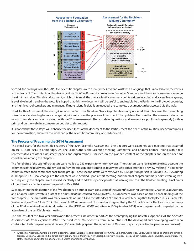
The Structure of the 2014 ReportThe previous SAP reports have served well the Parties to the Montreal Protocol, the scientific community, and the managers who deal with the research activities. However, the Montreal Protocol process has matured significantly and its needs have evolved. It was clear from the discussions between the Cochairs and both the Party representatives and the people involved in decision making that the previous very lengthy assessment reports would not meet the current needs of the Parties for a short, pithy, document that is written for them and not for the scientific community. Yet, it was also clear that the integrity of and the trust in the SAP reports come from the very thorough assessment of the science. Therefore, this 2014 Assessment was restructured to serve both purposes. The new structure is shown schematically below.
First, as in the past, a major scientific assessment process was carried out and the findings from these discussions and reviews constitute the five major chapters of the assessment foundation from the scientific community. This is shown on the left hand side of the diagram. The five scientific chapters are published only on the web but are an integral part of the 2014 SAP report to the Parties. Also, as discussed earlier, the assessment of the surface UV changes due to past ozone depletion or to projected future ozone levels is not included in this document. Readers are referred to the 2014 Environmental Effects Assessment Panel report for the UV discussion.
iii
Second, the findings from the SAP’s five scientific chapters were then synthesized and written in a language that is accessible to the Parties to the Protocol. The contents of the Assessment for Decision-Makers document—an Executive Summary and three sections—are shown on the right hand side. This short document, which contains all the major scientific summary points written in a clear and accessible language, is available in print and on the web. It is hoped that this new document will be useful to and usable by the Parties to the Protocol, countries, and high-level policymakers and managers. If more scientific details are needed, the complete document can be accessed via the web.
Third, for this Assessment, the Twenty Questions and Answers About the Ozone Layer has been only updated. This is because the overarching scientific understanding has not changed significantly from the previous Assessment. The update will ensure that the answers include the most current data and are consistent with the 2014 Assessment. These updated questions and answers are published separately (both in print and on the web) in a companion booklet to this report.
It is hoped that these steps will enhance the usefulness of the document to the Parties, meet the needs of the multiple user communities for the information, minimize the workload of the scientific community, and reduce costs.
The Process of Preparing the 2014 AssessmentThe initial plans for the scientific chapters of the 2014 Scientific Assessment Panel’s report were examined at a meeting that occurred on 10–11 June 2013 in Cambridge, UK. The Lead Authors, the Scientific Steering Committee, and Chapter Editors—along with a few representatives of other assessment panels and organizations—focused on the planned content of the chapters and on the need for coordination among the chapters.
The first drafts of the scientific chapters were mailed to 213 experts for written reviews. The chapters were revised to take into account the comments of the reviewers. The revised drafts were subsequently sent to 65 reviewers who either attended a review meeting in Boulder or communicated their comments back to the group. These second drafts were reviewed by 63 experts in person in Boulder, CO, USA during 8–10 April 2014. Final changes to the chapters were decided upon at this meeting, and the final chapter summary points were agreed. Subsequently, the chapters were revised for clarity and to address specific points that were agreed to at the Boulder meeting. Final drafts of the scientific chapters were completed in May 2014.
Subsequent to the finalization of the five chapters, an author team consisting of the Scientific Steering Committee, Chapter Lead Authors, and Chapter Editors wrote a draft of the Assessment for Decision-Makers (ADM). This document was based on the science findings of the five chapters. The draft ADM was made available on June 13 to the attendees of a Panel Review Meeting that took place in Les Diablerets, Switzerland, on 23–27 June 2014. The overall ADM was reviewed, discussed, and agreed to by the 59 participants. The Executive Summary of the ADM, contained herein (and posted on the UNEP and WMO websites on 10 September 2014), was prepared and completed by the attendees of the Les Diablerets meeting.
The final result of this two-year endeavor is the present assessment report. As the accompanying list indicates (Appendix A), the Scientific Assessment of Ozone Depletion: 2014 is the product of 285 scientists from 36 countries4 of the developed and developing world who contributed to its preparation and review (130 scientists prepared the report and 220 scientists participated in the peer review process).
4 Argentina, Australia, Austria, Belgium, Botswana, Brazil, Canada, People’s Republic of China, Comoros, Costa Rica, Cuba, Czech Republic, Denmark, Finland, France, Germany, Greece, India, Israel, Italy, Japan, Korea, Malaysia, New Zealand, Norway, Poland, Russia, South Africa, Spain, Sweden, Switzerland, The Netherlands, Togo, United Kingdom, United States of America, Zimbabwe.

v
ContentsExecutive Summary ES-1
Preface i
Introduction 1
Policy-Relevant Highlights from the 2014 Ozone Assessment 3
1. Current State of Ozone-Depleting Substances, Their Substitutes, and the Ozone Layer 5
2. Future Issues Regarding Ozone-Depleting Substances and Their Substitutes 15
3. Evolution of the Global Ozone Layer 19
4. Evolution of Polar Ozone 23
5. Past Stratospheric Ozone Changes and Climate 27
6. The Future of the Ozone Layer 29
Additional Information of Interest to Decision-Makers 33
Metrics for Changes in Ozone and Climate 35
Scenarios and Sensitivity Analyses 41
Appendices A-1
A. Authors, Contributors, Reviewers, and Other Participants in the 2014 Ozone Assessment A-3
B. Chapter Scientific Summaries A-9
C. Atmospheric Lifetimes for Selected Long-Lived Halocarbons A-21
D. Ozone Depletion Potentials (ODPs) for Long-Lived Halocarbons A-22
E. Estimated Ozone Depletion Potentials (ODPs) for Short-Lived Halocarbons as a Function of Their Emissions Location A-23
F. Global Warming Potentials (GWPs) and Global Temperature change Potentials (GTPs) of Various Halocarbons A-24
G. Lifetime and Full Uncertainty Estimates of Global Warming Potentials (GWPs) of Selected Hydrofluorocarbons (HFCs) A-25
H. Indirect Global Warming Potentials (GWPs) from Ozone Depletion A-26
I. Mixing Ratios of the ODSs Considered in the Baseline (A1) Scenario A-27
J. Acronyms A-29
K. Chemical Formulae A-31

1
The science of the stratospheric ozone layer and the ability to forecast its future have greatly advanced over the past few decades. In concert with this scientific development, the policy to avoid and mitigate ozone layer depletion has been successfully developed and implemented by the Montreal Protocol and its many Amendments and adjustments. The Protocol mandated periodic reports on the state of the ozone layer, ozone-depleting substances, and the future of the ozone layer. The Scientific Assessment Panel (SAP) was charged to prepare the reports under the auspices of the United Nations Environment Programme and the World Meteorological Organization. This quadrennial assessment of the science of the ozone layer has been one of the key components of the architecture of this science-policy enterprise. The SAP has also produced interim reports over the past decades on specific topics requested by the Parties. In addition, reports produced prior to the adoption of the Montreal Protocol helped pave the way for the Protocol and the SAP.
Findings of the Previous (2010) SAP ReportThis 2014 report is the eighth full report by the SAP. To place the current Assessment in context, we briefly recap the major conclusions of the previous (2010) report:
• By successfully controlling the emissions of ozone-depleting substances (ODSs), the Montreal Protocol has protected the ozone layer from much higher levels of depletion. The Montreal Protocol also has had co-benefits for climate, because many ODSs are also greenhouse gases.
• The abundances of ODSs in the atmosphere are responding as expected to the controls of the Montreal Protocol.
• Atmospheric observations of ozone continue to show that the ozone layer is not depleting further, but it is too soon to determine if the recovery has started.
• The ozone layer and climate change are intricately coupled, and climate change will become increasingly more important to the future of the ozone layer.
• The impact of the Antarctic ozone hole on surface climate is becoming evident.
• The ozone layer and surface ultraviolet (UV) radiation are responding as expected to the ODS reductions achieved under the Montreal Protocol.
• Options for further limiting future emissions of ODSs could advance recovery dates by a few years; however, the impact on future ozone levels would be less than what has already been accomplished by the Montreal Protocol.
The 2014 SAP Report and Its Assessment for Decision-MakersThe five scientific chapters of the 2014 report build on the findings of the 2010 report and its predecessors. The information from the 2014 scientific chapters has been synthesized in this Assessment for Decision-Makers (ADM). All the findings of the ADM are traceable to the five scientific chapters.
The ADM has a high-level Executive Summary and policy-relevant highlights from the scientific chapters, presented in three levels of detail. Addtional information that is useful for decision-makers is also included. Appendices contain the key findings of all the scientific chapters, as well as additional tables.
Introduction

3
This section of the Assessment for Decision-Makers presents policy-relevant highlights from the five scientific chapters of the 2014 Assessment. A high-level overarching finding appears in a light blue box at the start of each of the six topics shown above. Each of the six topics then presents major highlights in yellow boxes, with some additional information following the yellow highlights. This format allows the document to be viewed at various levels—a quick read of the six overarching findings (blue boxes) to get an overview of the state of the ozone layer issue, as well as a more detailed read of the highlights relevant to decision-makers (yellow boxes and their supporting detail). The underlying chapter material for the major highlights is indicated in [blue brackets]. See the relevant chapter for any cited references, figures, tables, and sections.
1. Current State of Ozone-Depleting Substances, Their Substitutes, and the Ozone Layer
2. Future Issues Regarding Ozone-Depleting Substances and Their Substitutes
3. Evolution of the Global Ozone Layer
4. Evolution of Polar Ozone
5. Past Stratospheric Ozone Changes and Climate
6. The Future of the Ozone Layer
POLICY-RELEVANT HIGHLIGHTS FROMTHE 2014 OZONE ASSESSMENT

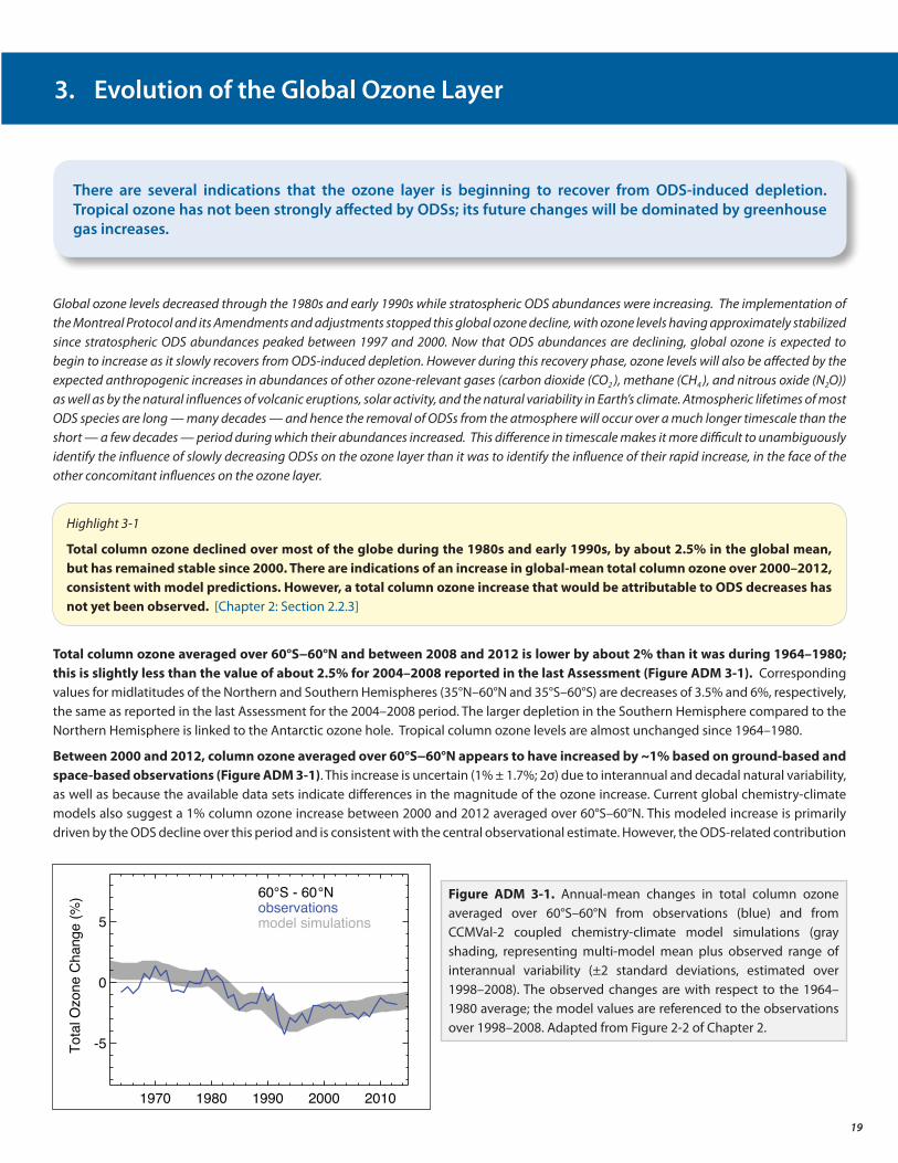
5
Compliance with the Montreal Protocol is assessed in this report based on the measured abundances of controlled ozone-depleting substances (ODSs) in the troposphere from ground-based networks. Observations of atmospheric abundances of these chemicals and their degradation products also come from: episodic airborne and ground-based “snapshot” measurements; ground-based overhead column and profile measurements of tropospheric and stratospheric abundances; stratospheric balloon-borne and airborne measurements; and satellite-based measurements that provide global coverage. The tropospheric abundances of ODSs are used with modeling calculations to estimate stratospheric abundances of chlorine- and bromine-containing chemicals, which are checked against measurements from satellite, ground-based, and episodic aircraft and balloon-borne instruments. Fluorinated chemicals produced from the degradation of ODSs and their substitutes do not deplete ozone. They are also measured and tracked, as they provide another consistency check on the measured abundances of the ODSs.
Reconciliation of the observed tropospheric abundances of the ODSs with their known emission inventory requires values of their atmospheric lifetimes. The lifetimes are, in general, quantified using laboratory data, atmospheric observations, and atmospheric model calculations. If the lifetime of an individual species is known, the observed atmospheric abundance can be used to derive its historical global emission.
The data sets obtained are used to calculate the effects of ODSs, ODS substitutes, and related chemicals on stratospheric ozone (via the Equivalent Effective Stratospheric Chlorine (EESC) and Ozone Depletion Potential (ODP)-weighted emissions; see Box ADM 1-1) and Earth’s climate (via changes in radiative forcing (RF) and Global Warming Potential (GWP)-weighted emissions; see Box ADM 1-2). The tropospheric abundances are also used as key input to chemistry-climate models to calculate past, present, and future levels of stratospheric ozone abundances.
Future ODS levels depend on future production, emissions from existing banks (which are ODSs that have already been manufactured but not yet released to the atmosphere), and how quickly the atmosphere is cleansed of ODSs already there. The last factor requires knowledge of the atmospheric lifetimes of the individual ODSs. The baseline scenario assumes that controlled ODS emissions will be limited to future production allowed by the Montreal Protocol (complete compliance with the current agreement), and that there are no further Amendments and adjustments (e.g., the uncontrollable emissions from banks are left as they are). Clearly, future ODS levels could be further reduced by reducing or eliminating future production and/or recovering existing banks. The potential gains from such actions are quantified by comparing the changes in EESC, ODP-weighted emissions, RF, and GWP-weighted emissions for the different scenarios.
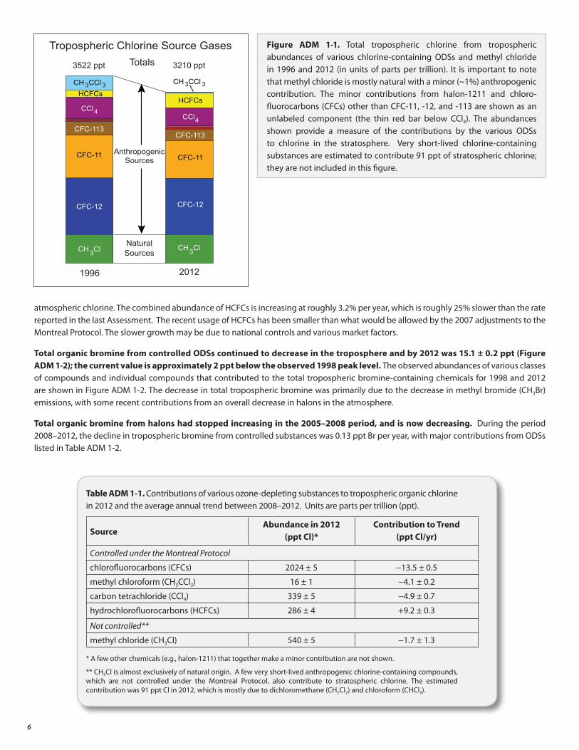
Total tropospheric organic chlorine from methyl chloride (CH3Cl) and controlled ODSs 5 continued to decrease between 1996 and 2012, reaching 3210 parts per trillion (ppt) in 2012. The observed abundances of various classes of compounds and individual compounds that contributed to the total tropospheric chlorine between the two years are shown in Figure ADM 1-1.
During the period 2008–2012, the decline in tropospheric chlorine from controlled substances was 13.4 ± 0.9 ppt per year 6, with major contributions from ODSs listed in Table ADM 1-1. The annual rate of decrease in the sum of chlorine during this period is about 50% smaller than the maximum annual decrease rate observed between 1996 and 2001, the period when the atmospheric abundance of methyl chloroform was declining more rapidly.
Increasing hydrochlorofluorocarbon (HCFC) abundances partially offset the tropospheric chlorine decline from decreasing levels of CFCs, carbon tetrachloride (CCl4), and methyl chloroform (CH3CCl3). HCFCs accounted for 286 ± 4 ppt of the total current
1. Current State of Ozone-Depleting Substances, Their Substitutes, and the Ozone Layer
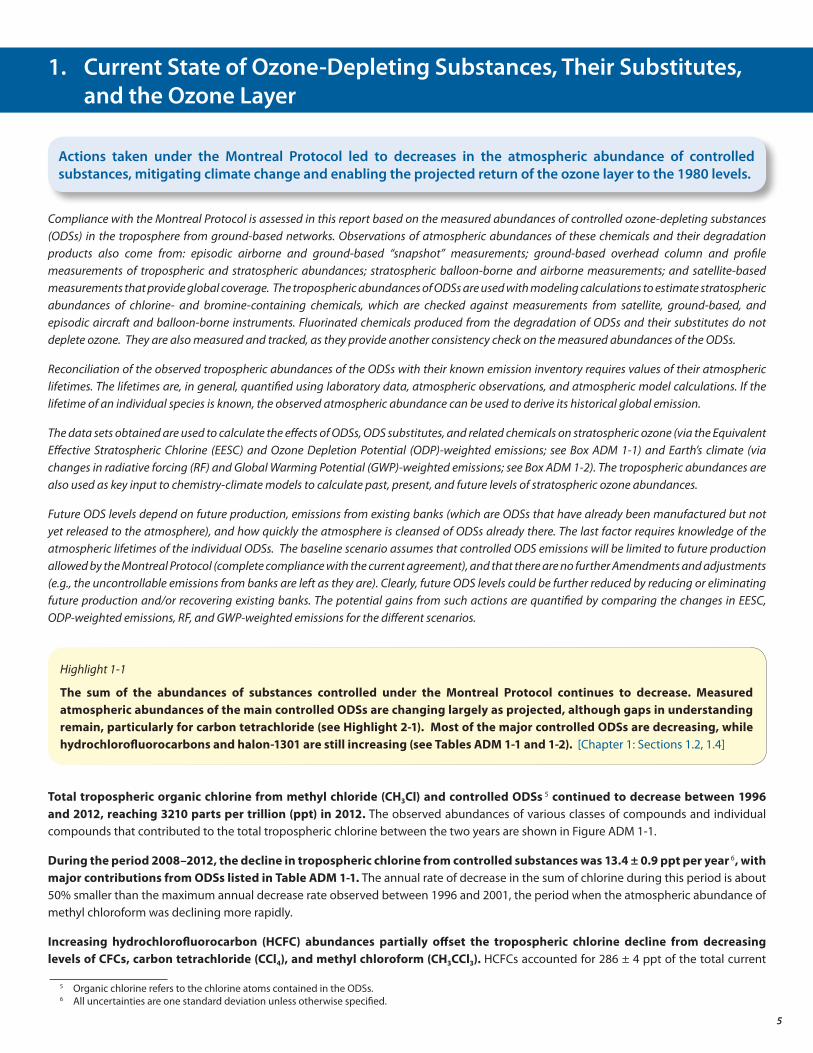
Actions taken under the Montreal Protocol led to decreases in the atmospheric abundance of controlled substances, mitigating climate change and enabling the projected return of the ozone layer to the 1980 levels.
Highlight 1-1
The sum of the abundances of substances controlled under the Montreal Protocol continues to decrease. Measured atmospheric abundances of the main controlled ODSs are changing largely as projected, although gaps in understanding remain, particularly for carbon tetrachloride (see Highlight 2-1). Most of the major controlled ODSs are decreasing, while hydrochlorofluorocarbons and halon-1301 are still increasing (see Tables ADM 1-1 and 1-2). [Chapter 1: Sections 1.2, 1.4]
5 Organic chlorine refers to the chlorine atoms contained in the ODSs.6 All uncertainties are one standard deviation unless otherwise specified.
6
atmospheric chlorine. The combined abundance of HCFCs is increasing at roughly 3.2% per year, which is roughly 25% slower than the rate reported in the last Assessment. The recent usage of HCFCs has been smaller than what would be allowed by the 2007 adjustments to the Montreal Protocol. The slower growth may be due to national controls and various market factors.
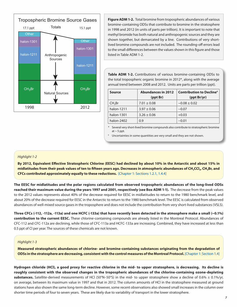
Total organic bromine from controlled ODSs continued to decrease in the troposphere and by 2012 was 15.1 ± 0.2 ppt (Figure ADM 1-2); the current value is approximately 2 ppt below the observed 1998 peak level. The observed abundances of various classes of compounds and individual compounds that contributed to the total tropospheric bromine-containing chemicals for 1998 and 2012 are shown in Figure ADM 1-2. The decrease in total tropospheric bromine was primarily due to the decrease in methyl bromide (CH3Br) emissions, with some recent contributions from an overall decrease in halons in the atmosphere.
Total organic bromine from halons had stopped increasing in the 2005–2008 period, and is now decreasing. During the period 2008–2012, the decline in tropospheric bromine from controlled substances was 0.13 ppt Br per year, with major contributions from ODSs listed in Table ADM 1-2.
Table ADM 1-1. Contributions of various ozone-depleting substances to tropospheric organic chlorine in 2012 and the average annual trend between 2008–2012. Units are parts per trillion (ppt).
SourceAbundance in 2012
(ppt Cl)*Contribution to Trend
(ppt Cl/yr)
Controlled under the Montreal Protocol
chlorofluorocarbons (CFCs) 2024 ± 5 −13.5 ± 0.5
methyl chloroform (CH3CCl3) 16 ± 1 −4.1 ± 0.2
carbon tetrachloride (CCl4) 339 ± 5 −4.9 ± 0.7
hydrochlorofluorocarbons (HCFCs) 286 ± 4 +9.2 ± 0.3
Not controlled**
methyl chloride (CH3Cl) 540 ± 5 −1.7 ± 1.3
* A few other chemicals (e.g., halon-1211) that together make a minor contribution are not shown.
** CH3Cl is almost exclusively of natural origin. A few very short-lived anthropogenic chlorine-containing compounds, which are not controlled under the Montreal Protocol, also contribute to stratospheric chlorine. The estimated contribution was 91 ppt Cl in 2012, which is mostly due to dichloromethane (CH2Cl2) and chloroform (CHCl3).
CFC-11
CFC-12
CH 3Cl
CFC-113
CCl4
HCFCsCH 3CCl 3
Tropospheric Chlorine Source Gases
1996
3522 ppt Totals
CFC-11
CFC-12
CH 3Cl
CFC-113
CCl4
HCFCs
CH 3CCl 3
AnthropogenicSources
NaturalSources
3210 ppt
2012
Figure ADM 1-1. Total tropospheric chlorine from tropospheric abundances of various chlorine-containing ODSs and methyl chloride in 1996 and 2012 (in units of parts per trillion). It is important to note that methyl chloride is mostly natural with a minor (~1%) anthropogenic contribution. The minor contributions from halon-1211 and chloro-fluorocarbons (CFCs) other than CFC-11, -12, and -113 are shown as an unlabeled component (the thin red bar below CCl4). The abundances shown provide a measure of the contributions by the various ODSs to chlorine in the stratosphere. Very short-lived chlorine-containing substances are estimated to contribute 91 ppt of stratospheric chlorine; they are not included in this figure.
7
The EESC for midlatitudes and the polar regions calculated from observed tropospheric abundances of the long-lived ODSs reached their maximum value during the years 1997 and 2001, respectively (see Box ADM 1-1). The decrease from the peak values to the 2012 values represents about 40% of the decrease required for EESC in midlatitudes to return to the 1980 benchmark level, and about 20% of the decrease required for EESC in the Antarctic to return to the 1980 benchmark level. The EESC is calculated from observed abundances of well-mixed source gases in the troposphere and does not include the contribution from very short-lived substances (VSLS).
Three CFCs (-112, -112a, -113a) and one HCFC (-133a) that have recently been detected in the atmosphere make a small (~0.1%) contribution to the current EESC. These chlorine-containing compounds are already listed in the Montreal Protocol. Abundances of CFC-112 and CFC-112a are declining, while those of CFC-113a and HCFC-133a are increasing. Combined, they have increased at less than 0.5 ppt of Cl per year. The sources of these chemicals are not known.
Hydrogen chloride (HCl), a good proxy for reactive chlorine in the mid- to upper stratosphere, is decreasing. Its decline is roughly consistent with the observed changes in the tropospheric abundances of the chlorine-containing ozone-depleting substances. Satellite-derived measurements of HCl (50°N–50°S) in the mid- to upper stratosphere show a decline of 0.6% ± 0.1%/yr, on average, between its maximum value in 1997 and that in 2012. The column amounts of HCl in the stratosphere measured at ground stations have also shown the same long-term decline. However, some recent observations also showed small increases in the column over shorter time periods of four to seven years. These are likely due to variability of transport in the lower stratosphere.
Table ADM 1-2. Contributions of various bromine-containing ODSs to the total tropospheric organic bromine in 2012*, along with the average annual trend between 2008 and 2012. Units are parts per trillion (ppt).
Source Abundances in 2012 (ppt Br)
Contribution to Decline# (ppt Br/yr)
CH3Br 7.01 ± 0.08 −0.08 ± 0.02
halon-1211 3.97 ± 0.06 −0.07
halon-1301 3.26 ± 0.06 +0.03
halon-2402 0.9 −0.01
* Several very short-lived bromine compounds also contribute to stratospheric bromine at ~ 5 ppt. # Uncertainties in some quantities are very small and they are not shown.
Highlight 1-2
By 2012, Equivalent Effective Stratospheric Chlorine (EESC) had declined by about 10% in the Antarctic and about 15% in midlatitudes from their peak values of ten to fifteen years ago. Decreases in atmospheric abundances of CH3CCl3, CH3Br, and CFCs contributed approximately equally to these reductions. [Chapter 1: Sections 1.2.1, 1.4.4]
Highlight 1-3
Measured stratospheric abundances of chlorine- and bromine-containing substances originating from the degradation of ODSs in the stratosphere are decreasing, consistent with the control measures of the Montreal Protocol. [Chapter 1: Section 1.4]
Natural Sources
AnthropogenicSources
CH3BrCH3Br
halon-1301
halon-1211
halon-1211
halon-1301 Other
Other
Tropospheric Bromine Source GasesTotals
1998 2012
17.1 ppt 15.1 ppt
Figure ADM 1-2. Total bromine from tropospheric abundances of various bromine-containing ODSs that contribute to bromine in the stratosphere in 1998 and 2012 (in units of parts per trillion). It is important to note that methyl bromide has both natural and anthropogenic sources and they are shown together, but demarcated by a line. Contributions of very short-lived bromine compounds are not included. The rounding-off errors lead to the small differences between the values shown in this figure and those listed in Table ADM 1-2.
8
Box ADM 1-1: Ozone Depletion Metrics
Equivalent Effective Stratospheric Chlorine (EESC)
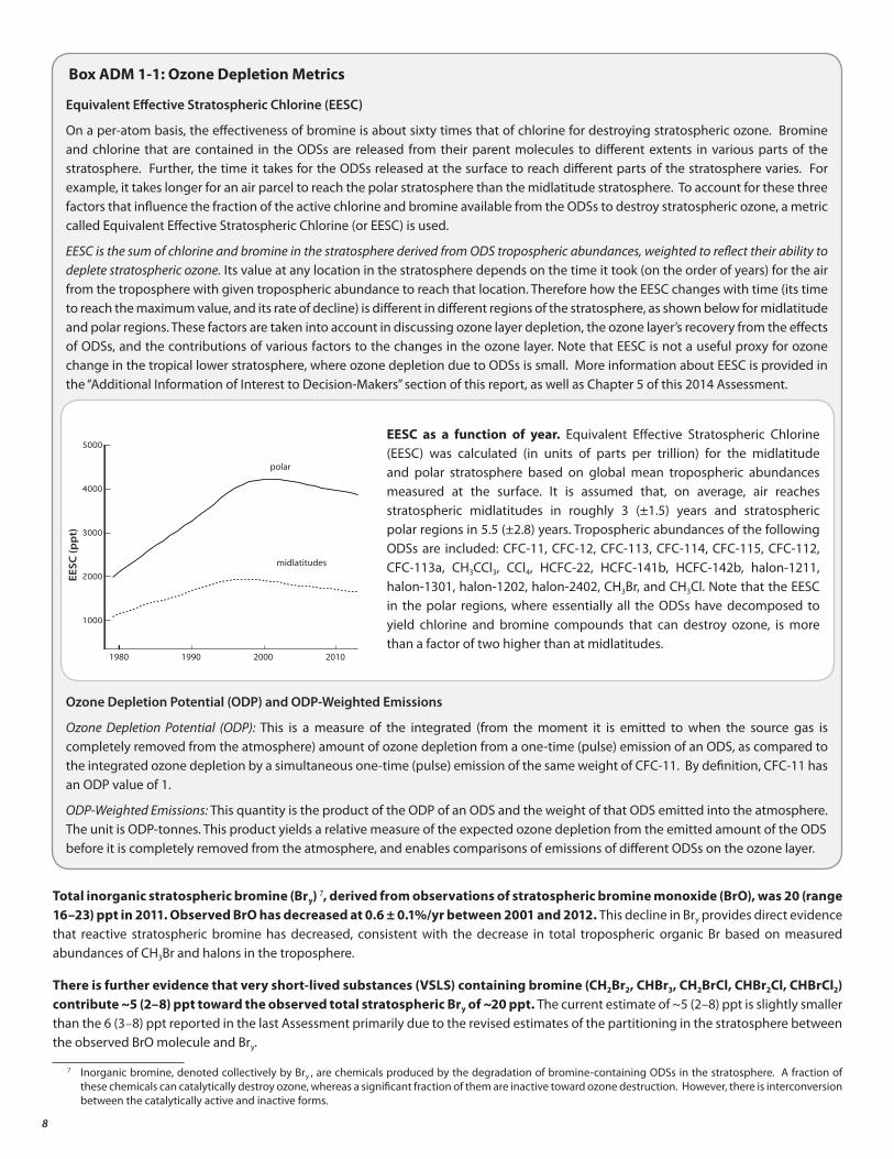
On a per-atom basis, the effectiveness of bromine is about sixty times that of chlorine for destroying stratospheric ozone. Bromine and chlorine that are contained in the ODSs are released from their parent molecules to different extents in various parts of the stratosphere. Further, the time it takes for the ODSs released at the surface to reach different parts of the stratosphere varies. For example, it takes longer for an air parcel to reach the polar stratosphere than the midlatitude stratosphere. To account for these three factors that influence the fraction of the active chlorine and bromine available from the ODSs to destroy stratospheric ozone, a metric called Equivalent Effective Stratospheric Chlorine (or EESC) is used.
EESC is the sum of chlorine and bromine in the stratosphere derived from ODS tropospheric abundances, weighted to reflect their ability to deplete stratospheric ozone. Its value at any location in the stratosphere depends on the time it took (on the order of years) for the air from the troposphere with given tropospheric abundance to reach that location. Therefore how the EESC changes with time (its time to reach the maximum value, and its rate of decline) is different in different regions of the stratosphere, as shown below for midlatitude and polar regions. These factors are taken into account in discussing ozone layer depletion, the ozone layer’s recovery from the effects of ODSs, and the contributions of various factors to the changes in the ozone layer. Note that EESC is not a useful proxy for ozone change in the tropical lower stratosphere, where ozone depletion due to ODSs is small. More information about EESC is provided in the “Additional Information of Interest to Decision-Makers” section of this report, as well as Chapter 5 of this 2014 Assessment.
Ozone Depletion Potential (ODP) and ODP-Weighted Emissions
Ozone Depletion Potential (ODP): This is a measure of the integrated (from the moment it is emitted to when the source gas is completely removed from the atmosphere) amount of ozone depletion from a one-time (pulse) emission of an ODS, as compared to the integrated ozone depletion by a simultaneous one-time (pulse) emission of the same weight of CFC-11. By definition, CFC-11 has an ODP value of 1.
ODP-Weighted Emissions: This quantity is the product of the ODP of an ODS and the weight of that ODS emitted into the atmosphere. The unit is ODP-tonnes. This product yields a relative measure of the expected ozone depletion from the emitted amount of the ODS before it is completely removed from the atmosphere, and enables comparisons of emissions of different ODSs on the ozone layer.
Total inorganic stratospheric bromine (Bry) 7, derived from observations of stratospheric bromine monoxide (BrO), was 20 (range 16–23) ppt in 2011. Observed BrO has decreased at 0.6 ± 0.1%/yr between 2001 and 2012. This decline in Bry provides direct evidence that reactive stratospheric bromine has decreased, consistent with the decrease in total tropospheric organic Br based on measured abundances of CH3Br and halons in the troposphere.
There is further evidence that very short-lived substances (VSLS) containing bromine (CH2Br2, CHBr3, CH2BrCl, CHBr2Cl, CHBrCl2) contribute ~5 (2–8) ppt toward the observed total stratospheric Bry of ~20 ppt. The current estimate of ~5 (2–8) ppt is slightly smaller than the 6 (3–8) ppt reported in the last Assessment primarily due to the revised estimates of the partitioning in the stratosphere between the observed BrO molecule and Bry.
1980 201020001990
EESC
(pp
t)
polar
midlatitudes
EESC as a function of year. Equivalent Effective Stratospheric Chlorine (EESC) was calculated (in units of parts per trillion) for the midlatitude and polar stratosphere based on global mean tropospheric abundances measured at the surface. It is assumed that, on average, air reaches stratospheric midlatitudes in roughly 3 (±1.5) years and stratospheric polar regions in 5.5 (±2.8) years. Tropospheric abundances of the following ODSs are included: CFC-11, CFC-12, CFC-113, CFC-114, CFC-115, CFC-112, CFC-113a, CH3CCl3, CCl4, HCFC-22, HCFC-141b, HCFC-142b, halon-1211, halon-1301, halon-1202, halon-2402, CH3Br, and CH3Cl. Note that the EESC in the polar regions, where essentially all the ODSs have decomposed to yield chlorine and bromine compounds that can destroy ozone, is more than a factor of two higher than at midlatitudes.
7 Inorganic bromine, denoted collectively by Bry , are chemicals produced by the degradation of bromine-containing ODSs in the stratosphere. A fraction of these chemicals can catalytically destroy ozone, whereas a significant fraction of them are inactive toward ozone destruction. However, there is interconversion between the catalytically active and inactive forms.
9
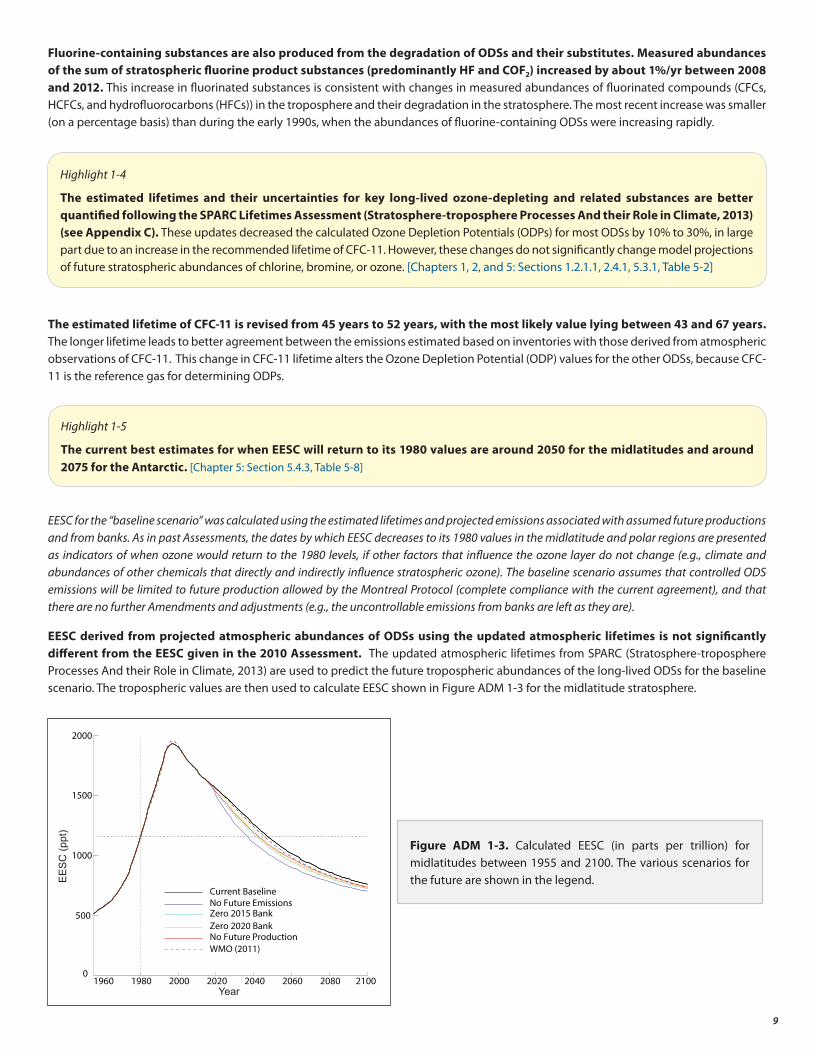
Figure ADM 1-3. Calculated EESC (in parts per trillion) for midlatitudes between 1955 and 2100. The various scenarios for the future are shown in the legend.
Fluorine-containing substances are also produced from the degradation of ODSs and their substitutes. Measured abundances of the sum of stratospheric fluorine product substances (predominantly HF and COF2) increased by about 1%/yr between 2008 and 2012. This increase in fluorinated substances is consistent with changes in measured abundances of fluorinated compounds (CFCs, HCFCs, and hydrofluorocarbons (HFCs)) in the troposphere and their degradation in the stratosphere. The most recent increase was smaller (on a percentage basis) than during the early 1990s, when the abundances of fluorine-containing ODSs were increasing rapidly.
The estimated lifetime of CFC-11 is revised from 45 years to 52 years, with the most likely value lying between 43 and 67 years. The longer lifetime leads to better agreement between the emissions estimated based on inventories with those derived from atmospheric observations of CFC-11. This change in CFC-11 lifetime alters the Ozone Depletion Potential (ODP) values for the other ODSs, because CFC-11 is the reference gas for determining ODPs.
EESC for the “baseline scenario” was calculated using the estimated lifetimes and projected emissions associated with assumed future productions and from banks. As in past Assessments, the dates by which EESC decreases to its 1980 values in the midlatitude and polar regions are presented as indicators of when ozone would return to the 1980 levels, if other factors that influence the ozone layer do not change (e.g., climate and abundances of other chemicals that directly and indirectly influence stratospheric ozone). The baseline scenario assumes that controlled ODS emissions will be limited to future production allowed by the Montreal Protocol (complete compliance with the current agreement), and that there are no further Amendments and adjustments (e.g., the uncontrollable emissions from banks are left as they are).
EESC derived from projected atmospheric abundances of ODSs using the updated atmospheric lifetimes is not significantly different from the EESC given in the 2010 Assessment. The updated atmospheric lifetimes from SPARC (Stratosphere-troposphere Processes And their Role in Climate, 2013) are used to predict the future tropospheric abundances of the long-lived ODSs for the baseline scenario. The tropospheric values are then used to calculate EESC shown in Figure ADM 1-3 for the midlatitude stratosphere.
1960 1980 2000 2020 2040 2060 2080 21000
500
1000
1500
2000
Current BaselineNo Future EmissionsZero 2015 BankZero 2020 BankNo Future ProductionWMO (2011)
Year
EE
SC
(ppt
)
Highlight 1-5
The current best estimates for when EESC will return to its 1980 values are around 2050 for the midlatitudes and around 2075 for the Antarctic. [Chapter 5: Section 5.4.3, Table 5-8]
Highlight 1-4
The estimated lifetimes and their uncertainties for key long-lived ozone-depleting and related substances are better quantified following the SPARC Lifetimes Assessment (Stratosphere-troposphere Processes And their Role in Climate, 2013) (see Appendix C). These updates decreased the calculated Ozone Depletion Potentials (ODPs) for most ODSs by 10% to 30%, in large part due to an increase in the recommended lifetime of CFC-11. However, these changes do not significantly change model projections of future stratospheric abundances of chlorine, bromine, or ozone. [Chapters 1, 2, and 5: Sections 1.2.1.1, 2.4.1, 5.3.1, Table 5-2]
10
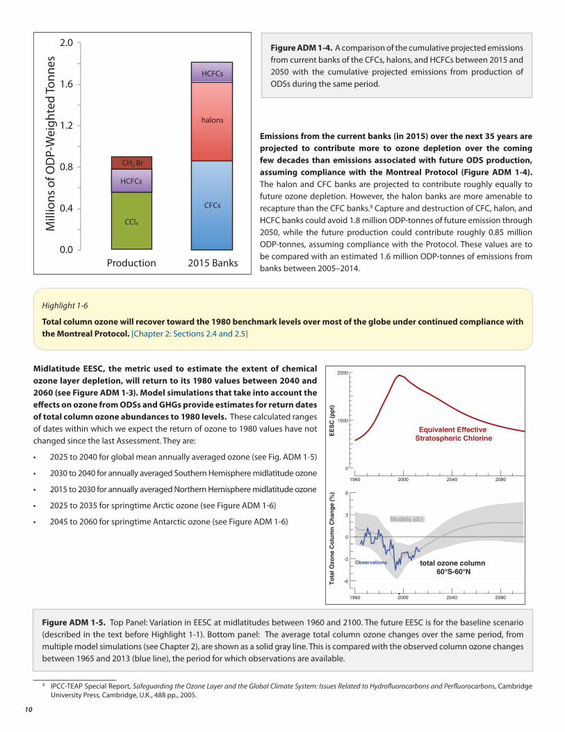
Emissions from the current banks (in 2015) over the next 35 years are projected to contribute more to ozone depletion over the coming few decades than emissions associated with future ODS production, assuming compliance with the Montreal Protocol (Figure ADM 1-4). The halon and CFC banks are projected to contribute roughly equally to future ozone depletion. However, the halon banks are more amenable to recapture than the CFC banks.8 Capture and destruction of CFC, halon, and HCFC banks could avoid 1.8 million ODP-tonnes of future emission through 2050, while the future production could contribute roughly 0.85 million ODP-tonnes, assuming compliance with the Protocol. These values are to be compared with an estimated 1.6 million ODP-tonnes of emissions from banks between 2005–2014.
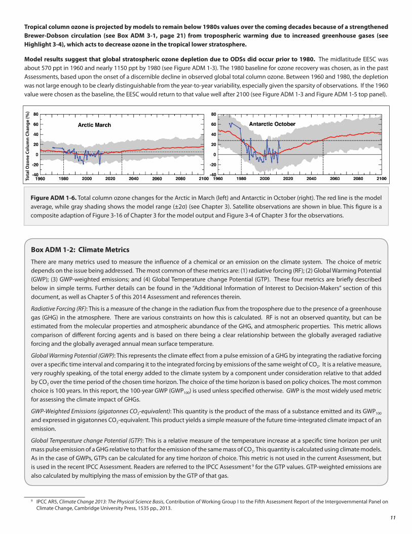
Midlatitude EESC, the metric used to estimate the extent of chemical ozone layer depletion, will return to its 1980 values between 2040 and 2060 (see Figure ADM 1-3). Model simulations that take into account the effects on ozone from ODSs and GHGs provide estimates for return dates of total column ozone abundances to 1980 levels. These calculated ranges of dates within which we expect the return of ozone to 1980 values have not changed since the last Assessment. They are:
• 2025 to 2040 for global mean annually averaged ozone (see Fig. ADM 1-5)
• 2030 to 2040 for annually averaged Southern Hemisphere midlatitude ozone
• 2015 to 2030 for annually averaged Northern Hemisphere midlatitude ozone
• 2025 to 2035 for springtime Arctic ozone (see Figure ADM 1-6)
• 2045 to 2060 for springtime Antarctic ozone (see Figure ADM 1-6)
Highlight 1-6
Total column ozone will recover toward the 1980 benchmark levels over most of the globe under continued compliance with the Montreal Protocol. [Chapter 2: Sections 2.4 and 2.5]
CCl4
CH Br3
HCFCs
halons
CFCs
HCFCs
HCFCs
2.0
0.8
0.4
1.2
1.6
0.0Production 2015 Banks
Mill
ions
of O
DP-
Wei
ghte
d To
nnes
Figure ADM 1-4. A comparison of the cumulative projected emissions from current banks of the CFCs, halons, and HCFCs between 2015 and 2050 with the cumulative projected emissions from production of ODSs during the same period.
-6
-3
0
3
6
Tota
l Ozo
ne C
olum
n Ch
ange
(%)
Models ±2σ
Observations
1960
0
1000
2000
EESC
(ppt
)
Equivalent EffectiveStratospheric Chlorine
total ozone column 60°S-60°N
2000 2040 2080
1960 2000 2040 2080
Figure ADM 1-5. Top Panel: Variation in EESC at midlatitudes between 1960 and 2100. The future EESC is for the baseline scenario (described in the text before Highlight 1-1). Bottom panel: The average total column ozone changes over the same period, from multiple model simulations (see Chapter 2), are shown as a solid gray line. This is compared with the observed column ozone changes between 1965 and 2013 (blue line), the period for which observations are available.
8 IPCC-TEAP Special Report, Safeguarding the Ozone Layer and the Global Climate System: Issues Related to Hydrofluorocarbons and Perfluorocarbons, Cambridge University Press, Cambridge, U.K., 488 pp., 2005.
11
Tropical column ozone is projected by models to remain below 1980s values over the coming decades because of a strengthened Brewer-Dobson circulation (see Box ADM 3-1, page 21) from tropospheric warming due to increased greenhouse gases (see Highlight 3-4), which acts to decrease ozone in the tropical lower stratosphere.
Model results suggest that global stratospheric ozone depletion due to ODSs did occur prior to 1980. The midlatitude EESC was about 570 ppt in 1960 and nearly 1150 ppt by 1980 (see Figure ADM 1-3). The 1980 baseline for ozone recovery was chosen, as in the past Assessments, based upon the onset of a discernible decline in observed global total column ozone. Between 1960 and 1980, the depletion was not large enough to be clearly distinguishable from the year-to-year variability, especially given the sparsity of observations. If the 1960 value were chosen as the baseline, the EESC would return to that value well after 2100 (see Figure ADM 1-3 and Figure ADM 1-5 top panel).
Box ADM 1-2: Climate Metrics
There are many metrics used to measure the influence of a chemical or an emission on the climate system. The choice of metric depends on the issue being addressed. The most common of these metrics are: (1) radiative forcing (RF); (2) Global Warming Potential (GWP); (3) GWP-weighted emissions; and (4) Global Temperature change Potential (GTP). These four metrics are briefly described below in simple terms. Further details can be found in the “Additional Information of Interest to Decision-Makers” section of this document, as well as Chapter 5 of this 2014 Assessment and references therein.
Radiative Forcing (RF): This is a measure of the change in the radiation flux from the troposphere due to the presence of a greenhouse gas (GHG) in the atmosphere. There are various constraints on how this is calculated. RF is not an observed quantity, but can be estimated from the molecular properties and atmospheric abundance of the GHG, and atmospheric properties. This metric allows comparison of different forcing agents and is based on there being a clear relationship between the globally averaged radiative forcing and the globally averaged annual mean surface temperature.
Global Warming Potential (GWP): This represents the climate effect from a pulse emission of a GHG by integrating the radiative forcing over a specific time interval and comparing it to the integrated forcing by emissions of the same weight of CO2. It is a relative measure, very roughly speaking, of the total energy added to the climate system by a component under consideration relative to that added by CO2 over the time period of the chosen time horizon. The choice of the time horizon is based on policy choices. The most common choice is 100 years. In this report, the 100-year GWP (GWP100) is used unless specified otherwise. GWP is the most widely used metric for assessing the climate impact of GHGs.
GWP-Weighted Emissions (gigatonnes CO2-equivalent): This quantity is the product of the mass of a substance emitted and its GWP100 and expressed in gigatonnes CO2-equivalent. This product yields a simple measure of the future time-integrated climate impact of an emission.
Global Temperature change Potential (GTP): This is a relative measure of the temperature increase at a specific time horizon per unit mass pulse emission of a GHG relative to that for the emission of the same mass of CO2. This quantity is calculated using climate models. As in the case of GWPs, GTPs can be calculated for any time horizon of choice. This metric is not used in the current Assessment, but is used in the recent IPCC Assessment. Readers are referred to the IPCC Assessment 9 for the GTP values. GTP-weighted emissions are also calculated by multiplying the mass of emission by the GTP of that gas.
Tota
l Ozo
ne C
olum
n Ch
ange
(%)
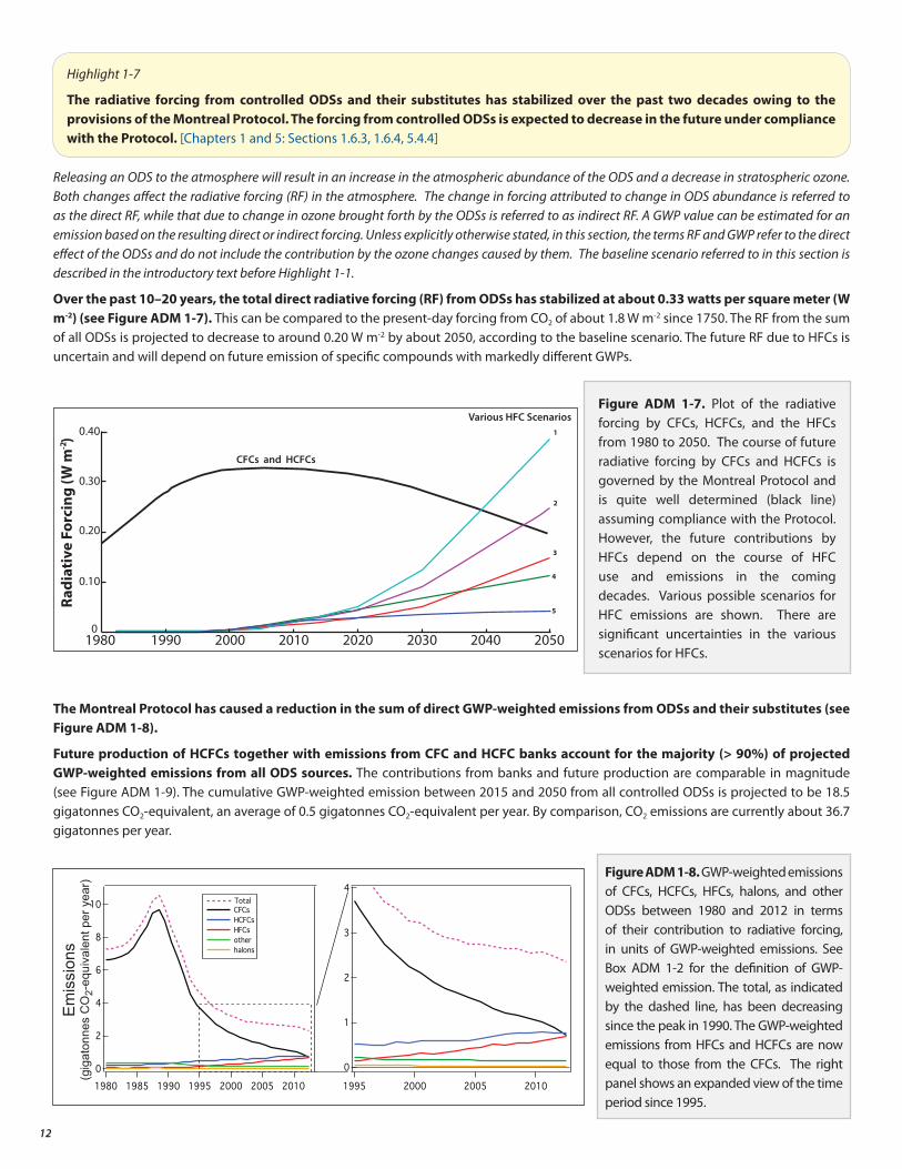
Figure ADM 1-6. Total column ozone changes for the Arctic in March (left) and Antarctic in October (right). The red line is the model average, while gray shading shows the model range (±2σ) (see Chapter 3). Satellite observations are shown in blue. This figure is a composite adaption of Figure 3-16 of Chapter 3 for the model output and Figure 3-4 of Chapter 3 for the observations.
9 IPCC AR5, Climate Change 2013: The Physical Science Basis, Contribution of Working Group I to the Fifth Assessment Report of the Intergovernmental Panel on Climate Change, Cambridge University Press, 1535 pp., 2013.
12
Releasing an ODS to the atmosphere will result in an increase in the atmospheric abundance of the ODS and a decrease in stratospheric ozone. Both changes affect the radiative forcing (RF) in the atmosphere. The change in forcing attributed to change in ODS abundance is referred to as the direct RF, while that due to change in ozone brought forth by the ODSs is referred to as indirect RF. A GWP value can be estimated for an emission based on the resulting direct or indirect forcing. Unless explicitly otherwise stated, in this section, the terms RF and GWP refer to the direct effect of the ODSs and do not include the contribution by the ozone changes caused by them. The baseline scenario referred to in this section is described in the introductory text before Highlight 1-1.
Over the past 10–20 years, the total direct radiative forcing (RF) from ODSs has stabilized at about 0.33 watts per square meter (W m-2) (see Figure ADM 1-7). This can be compared to the present-day forcing from CO2 of about 1.8 W m-2 since 1750. The RF from the sum of all ODSs is projected to decrease to around 0.20 W m-2 by about 2050, according to the baseline scenario. The future RF due to HFCs is uncertain and will depend on future emission of specific compounds with markedly different GWPs.
The Montreal Protocol has caused a reduction in the sum of direct GWP-weighted emissions from ODSs and their substitutes (see Figure ADM 1-8).
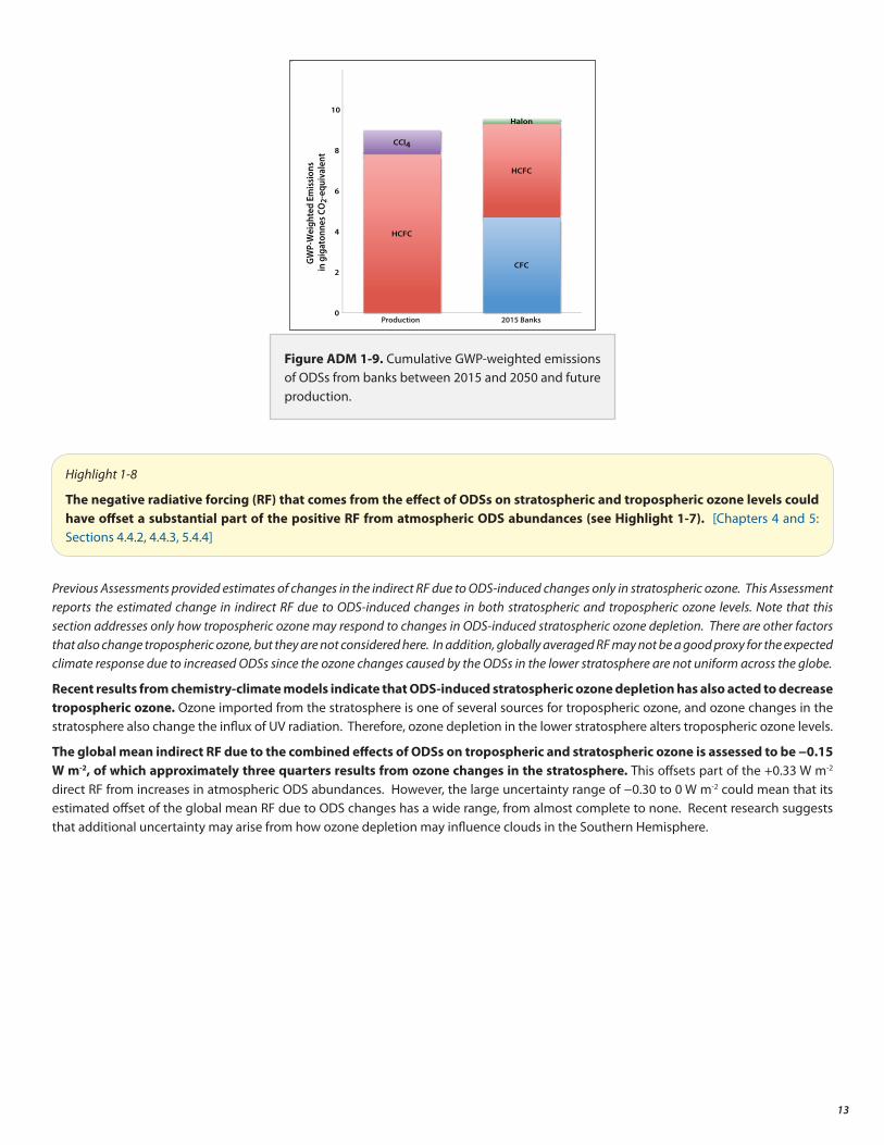
Future production of HCFCs together with emissions from CFC and HCFC banks account for the majority (> 90%) of projected GWP-weighted emissions from all ODS sources. The contributions from banks and future production are comparable in magnitude (see Figure ADM 1-9). The cumulative GWP-weighted emission between 2015 and 2050 from all controlled ODSs is projected to be 18.5 gigatonnes CO2-equivalent, an average of 0.5 gigatonnes CO2-equivalent per year. By comparison, CO2 emissions are currently about 36.7 gigatonnes per year.
Highlight 1-7
The radiative forcing from controlled ODSs and their substitutes has stabilized over the past two decades owing to the provisions of the Montreal Protocol. The forcing from controlled ODSs is expected to decrease in the future under compliance with the Protocol. [Chapters 1 and 5: Sections 1.6.3, 1.6.4, 5.4.4]
4
2
3
1
5
Radi
ativ
e Fo
rcin
g (W
m )-2
0
0.10
0.20
0.30
0.40
1980 1990 2000 2010 2020 2030 2040 2050
CFCs and HCFCs
Various HFC ScenariosFigure ADM 1-7. Plot of the radiative forcing by CFCs, HCFCs, and the HFCs from 1980 to 2050. The course of future radiative forcing by CFCs and HCFCs is governed by the Montreal Protocol and is quite well determined (black line) assuming compliance with the Protocol. However, the future contributions by HFCs depend on the course of HFC use and emissions in the coming decades. Various possible scenarios for HFC emissions are shown. There are significant uncertainties in the various scenarios for HFCs.
Em
issi
ons
(gig
aton
nes
CO
2-eq
uiva
lent
per
yea
r)
Figure ADM 1-8. GWP-weighted emissions of CFCs, HCFCs, HFCs, halons, and other ODSs between 1980 and 2012 in terms of their contribution to radiative forcing, in units of GWP-weighted emissions. See Box ADM 1-2 for the definition of GWP-weighted emission. The total, as indicated by the dashed line, has been decreasing since the peak in 1990. The GWP-weighted emissions from HFCs and HCFCs are now equal to those from the CFCs. The right panel shows an expanded view of the time period since 1995.
13
Previous Assessments provided estimates of changes in the indirect RF due to ODS-induced changes only in stratospheric ozone. This Assessment reports the estimated change in indirect RF due to ODS-induced changes in both stratospheric and tropospheric ozone levels. Note that this section addresses only how tropospheric ozone may respond to changes in ODS-induced stratospheric ozone depletion. There are other factors that also change tropospheric ozone, but they are not considered here. In addition, globally averaged RF may not be a good proxy for the expected climate response due to increased ODSs since the ozone changes caused by the ODSs in the lower stratosphere are not uniform across the globe.
Recent results from chemistry-climate models indicate that ODS-induced stratospheric ozone depletion has also acted to decrease tropospheric ozone. Ozone imported from the stratosphere is one of several sources for tropospheric ozone, and ozone changes in the stratosphere also change the influx of UV radiation. Therefore, ozone depletion in the lower stratosphere alters tropospheric ozone levels.
The global mean indirect RF due to the combined effects of ODSs on tropospheric and stratospheric ozone is assessed to be −0.15 W m-2, of which approximately three quarters results from ozone changes in the stratosphere. This offsets part of the +0.33 W m-2 direct RF from increases in atmospheric ODS abundances. However, the large uncertainty range of −0.30 to 0 W m-2 could mean that its estimated offset of the global mean RF due to ODS changes has a wide range, from almost complete to none. Recent research suggests that additional uncertainty may arise from how ozone depletion may influence clouds in the Southern Hemisphere.
CFC
HCFC
HCFC
CCl4
0
2
4
6
8
10
Produc sknaB 5102no
GW
P-W
eigh
ted
Emis
sion
s in
gig
aton
nes C
O2-
equi
vale
nt
Halon
Production 2015 Banks
Figure ADM 1-9. Cumulative GWP-weighted emissions of ODSs from banks between 2015 and 2050 and future production.
Highlight 1-8
The negative radiative forcing (RF) that comes from the effect of ODSs on stratospheric and tropospheric ozone levels could have offset a substantial part of the positive RF from atmospheric ODS abundances (see Highlight 1-7). [Chapters 4 and 5: Sections 4.4.2, 4.4.3, 5.4.4]

15
This section addresses a few key issues that were specifically requested by the Parties and those that bear watching in the coming years leading to the next Assessment. The details of the calculations and further information are given in the science chapters, but the essence of the information is captured here. The first topic deals with information on carbon tetrachloride (CCl4), which was requested by the Parties. The second topic relates to hydrochlorofluorocarbons (HCFCs) and methyl bromide (CH3Br), two substances that are controlled under the Montreal Protocol. This topic also includes chlorine- and bromine-containing very short-lived substances (VSLS), knowledge of which may enhance our ability to predict future Equivalent Effective Stratospheric Chlorine (EESC) from projected emissions. The third topic deals with hydrofluorocarbons (HFCs). HFCs are not ODSs since fluorine does not deplete the ozone layer. However, HFCs are related to ODSs because most HFCs in the atmosphere are from emissions associated with their use as ODS substitutes or unintended emissions from production of other chemicals (e.g., HFC-23 from HCFC-22 manufacture). For this reason, we also address the climate impacts from different HFC emission scenarios.
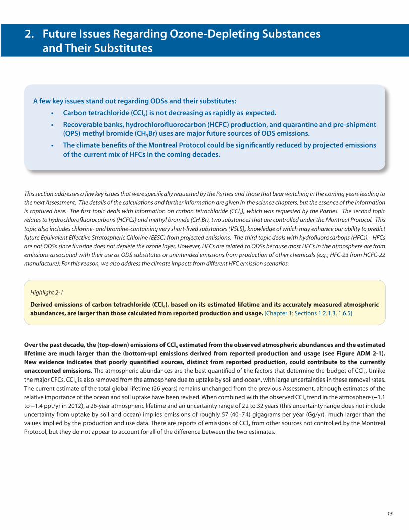
Over the past decade, the (top-down) emissions of CCl4 estimated from the observed atmospheric abundances and the estimated lifetime are much larger than the (bottom-up) emissions derived from reported production and usage (see Figure ADM 2-1). New evidence indicates that poorly quantified sources, distinct from reported production, could contribute to the currently unaccounted emissions. The atmospheric abundances are the best quantified of the factors that determine the budget of CCl4. Unlike the major CFCs, CCl4 is also removed from the atmosphere due to uptake by soil and ocean, with large uncertainties in these removal rates. The current estimate of the total global lifetime (26 years) remains unchanged from the previous Assessment, although estimates of the relative importance of the ocean and soil uptake have been revised. When combined with the observed CCl4 trend in the atmosphere (−1.1 to −1.4 ppt/yr in 2012), a 26-year atmospheric lifetime and an uncertainty range of 22 to 32 years (this uncertainty range does not include uncertainty from uptake by soil and ocean) implies emissions of roughly 57 (40–74) gigagrams per year (Gg/yr), much larger than the values implied by the production and use data. There are reports of emissions of CCl4 from other sources not controlled by the Montreal Protocol, but they do not appear to account for all of the difference between the two estimates.
A few key issues stand out regarding ODSs and their substitutes:
• Carbon tetrachloride (CCl4) is not decreasing as rapidly as expected.
• Recoverable banks, hydrochlorofluorocarbon (HCFC) production, and quarantine and pre-shipment (QPS) methyl bromide (CH3Br) uses are major future sources of ODS emissions.
• The climate benefits of the Montreal Protocol could be significantly reduced by projected emissions of the current mix of HFCs in the coming decades.
2. Future Issues Regarding Ozone-Depleting Substances and Their Substitutes
Highlight 2-1
Derived emissions of carbon tetrachloride (CCl4), based on its estimated lifetime and its accurately measured atmospheric abundances, are larger than those calculated from reported production and usage. [Chapter 1: Sections 1.2.1.3, 1.6.5]
16
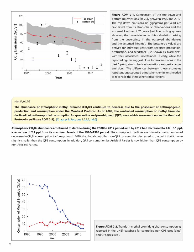
Atmospheric CH3Br abundances continued to decline during the 2008 to 2012 period, and by 2012 had decreased to 7.0 ± 0.1 ppt, a reduction of 2.2 ppt from its maximum levels of the 1996–1998 period. The atmospheric declines are primarily due to continued decreases in CH3Br consumption for fumigation. In 2010, the global controlled non-QPS consumption decreased to the point that it is now slightly smaller than the QPS consumption. In addition, QPS consumption by Article 5 Parties is now higher than QPS consumption by non-Article 5 Parties.
1995 2000 2005 2010
CCl 4 E
mis
sion
s (G
g/yr
)
Year
120
0
20
40
60
80
100
Figure ADM 2-1. Comparison of the top-down and bottom-up emissions for CCl4 between 1995 and 2012. The top-down emissions (in gigagrams per year) are calculated from its atmospheric observations and the assumed lifetime of 26 years (red line; with gray area showing the uncertainties in this calculation arising from the uncertainty in the observed abundances and the assumed lifetime). The bottom-up values are derived for individual years from reported production, destruction, and feedstock use shown as black dots, with their associated uncertainties. Clearly, while the reported figures suggest close to zero emissions in the past 6 years, atmospheric observations suggest a larger emission. The differences between these estimates represent unaccounted atmospheric emissions needed to reconcile the atmospheric observations.
70
60
50
40
30
20
10
01990 1995 2000 2005
Year
Cons
umpt
ion
of M
ethy
l Bro
mid
e (G
g/yr
)
2005 2010
Figure ADM 2-2. Trends in methyl bromide global consumption as reported in the UNEP database for controlled non-QPS uses (blue) and QPS uses (red).
Highlight 2-2
The abundance of atmospheric methyl bromide (CH3Br) continues to decrease due to the phase-out of anthropogenic production and consumption under the Montreal Protocol. As of 2009, the controlled consumption of methyl bromide declined below the reported consumption for quarantine and pre-shipment (QPS) uses, which are exempt under the Montreal Protocol (see Figure ADM 2-2). [Chapter 1: Sections 1.2.1.7, 1.6.6]
17
Emissions of biogenically produced bromine-containing substances may increase as a result of changes in the management of their human-related production (e.g., marine aquaculture).
Near-surface atmospheric abundances of dichloromethane (CH2Cl2), an uncontrolled substance that has predominantly anthropogenic sources, has increased by ~ 60% over the last decade. Currently it is offsetting about 10% of the decline in tropospheric Cl due to long-lived chlorinated substances controlled by the Montreal Protocol. CH2Cl2 and other short-lived chlorine substances make a very small contribution to total stratospheric chlorine in the current atmosphere.
The ozone depletion resulting from emissions of VSLS is strongly dependent on the geographic location and season of emission. Ozone depletion is larger if emissions occur in regions close to convective regions in the tropics, allowing for a more rapid and efficient transport of the VSLS into the stratosphere.
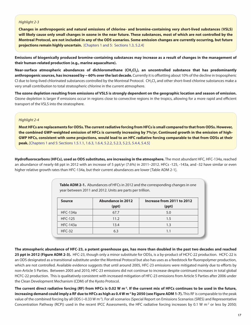
Hydrofluorocarbons (HFCs), used as ODS substitutes, are increasing in the atmosphere. The most abundant HFC, HFC-134a, reached an abundance of nearly 68 ppt in 2012 with an increase of 5 ppt/yr (7.6%) in 2011–2012. HFCs -125, -143a, and -32 have similar or even higher relative growth rates than HFC-134a, but their current abundances are lower [Table ADM 2-1].
Source Abundance in 2012(ppt)
Increase from 2011 to 2012(ppt)
HFC-134a 67.7 5.0
HFC-125 11.2 1.5
HFC-143a 13.4 1.3
HFC-32 6.3 1.1
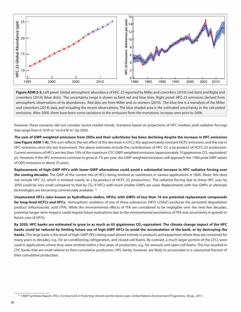
The atmospheric abundance of HFC-23, a potent greenhouse gas, has more than doubled in the past two decades and reached 25 ppt in 2012 (Figure ADM 2-3). HFC-23, though only a minor substitute for ODSs, is a by-product of HCFC-22 production. HCFC-22 is an ODS designated as a transitional substitute under the Montreal Protocol but also has uses as a feedstock for fluoropolymer production, which are not controlled. Available evidence suggests that until around 2005, HFC-23 emissions were mitigated mainly due to efforts by non-Article 5 Parties. Between 2005 and 2010, HFC-23 emissions did not continue to increase despite continued increases in total global HCFC-22 production. This is qualitatively consistent with increased mitigation of HFC-23 emissions from Article 5 Parties after 2006 under the Clean Development Mechanism (CDM) of the Kyoto Protocol.
The current direct radiative forcing (RF) from HFCs is 0.02 W m-2. If the current mix of HFCs continues to be used in the future, increasing demand could imply a RF due to HFCs as high as 0.4 W m-2 by 2050 (see Figure ADM 1-7). This RF is comparable to the peak value of the combined forcing by all ODS (~0.33 W m-2). For all scenarios (Special Report on Emissions Scenarios (SRES) and Representative Concentration Pathway (RCP)) used in the recent IPCC Assessments, the HFC radiative forcing increases by 0.1 W m-2 or less by 2050;
Highlight 2-3
Changes in anthropogenic and natural emissions of chlorine- and bromine-containing very short-lived substances (VSLS) will likely cause only small changes in ozone in the near future. These substances, most of which are not controlled by the Montreal Protocol, are not included in any of the ODS scenarios. Some emission changes are currently occurring, but future projections remain highly uncertain. [Chapters 1 and 5: Sections 1.3, 5.2.4]
Highlight 2-4
Most HFCs are replacements for ODSs. The current radiative forcing from HFCs is small compared to that from ODSs. However, the combined GWP-weighted emission of HFCs is currently increasing by 7%/yr. Continued growth in the emission of high-GWP HFCs, consistent with some projections, would lead to an HFC radiative forcing comparable to that from ODSs at their peak. [Chapters 1 and 5: Sections 1.5.1.1, 1.6.3, 1.6.4, 5.2.2, 5.2.3, 5.2.5, 5.4.4, 5.4.5]
Table ADM 2-1. Abundances of HFCs in 2012 and the corresponding changes in one year between 2011 and 2012. Units are parts per trillion.
18
however, these scenarios did not consider recent market trends. Scenarios based on projections of HFC markets yield radiative forcings that range from 0.16 W m-2 to 0.4 W m-2 by 2050.
The sum of GWP-weighted emissions from ODSs and their substitutes has been declining despite the increase in HFC emissions (see Figure ADM 1-8). This sum reflects the net effect of the decrease in CFCs, the approximately constant HCFC emissions, and the rise in HFC emissions since the last Assessment. The above estimates include the contributions of HFC-23, a by-product of HCFC-22 production. Current emissions of HFCs are less than 10% of the maximum CFC GWP-weighted emissions (approximately 10 gigatonnes CO2-equivalent/yr). However, if the HFC emissions continue to grow at 7% per year, the GWP-weighted emissions will approach the 1990 peak GWP values of ODS emissions in about 35 years.
Replacements of high-GWP HFCs with lower-GWP alternatives could avoid a substantial increase in HFC radiative forcing over the coming decades. The GWP of the current mix of HFCs being emitted as substitutes in various applications is 1600. (Note: this does not include HFC-23, which is emitted mainly as a by-product of HCFC-22 production.) The radiative forcing due to these HFC uses by 2050 could be very small compared to that by CO2 if HFCs with much smaller GWPs are used. Replacements with low GWPs or alternate technologies are becoming commercially available. 10
Unsaturated HFCs (also known as hydrofluoro-olefins, HFOs) with GWPs of less than 10 are potential replacement compounds for long-lived HCFCs and HFCs. Atmospheric oxidation of one of these substances (HFO-1234yf ) produces the persistent degradation product trifluoroacetic acid (TFA). While the environmental effects of TFA are considered to be negligible over the next few decades, potential longer-term impacts could require future evaluations due to the environmental persistence of TFA and uncertainty in growth in future uses of HFOs.
By 2050, HFC banks are estimated to grow to as much as 65 gigatonnes CO2-equivalent. The climate change impact of the HFC banks could be reduced by limiting future use of high-GWP HFCs to avoid the accumulation of the bank, or by destroying the banks. This large bank is the result of high-GWP HFCs being used almost entirely in products and equipment where they are contained for many years to decades, e.g., for air conditioning, refrigeration, and closed-cell foams. By contrast, a much larger portion of the CFCs were used in applications where they were emitted within a few years of production, e.g., for aerosols and open-cell foams. This has resulted in CFC banks that are small relative to their cumulative production. HFC banks, however, are likely to accumulate to a substantial fraction of their cumulative production.
10 UNEP Synthesis Report, HFCs: A Critical Link in Protecting Climate and the Ozone Layer, United Nations Environment Programme, 36 pp., 2011.
HFC
-23
Emis
sion
s (k
iloto
nnes
per
yea
r)
1980 201020052000199519901985
16
0
2
4
6
8
10
12
14
HFC
-23
Glo
bal A
bund
ance
(ppt
)
2010200520001995
25
10
15
20
Figure ADM 2-3. Left panel: Global atmospheric abundance of HFC-23 reported by Miller and coworkers (2010) (red dots) and Rigby and coworkers (2014) (blue dots). The uncertainty range is shown as faint red and blue lines. Right panel: HFC-23 emissions derived from atmospheric observations of its abundances. Red dots are from Miller and co-workers (2010). The blue line is a reanalysis of the Miller and coworkers (2014) data and including the recent observations. The blue shaded area is the estimated uncertainty in the calculated emissions. After 2000, there have been some variations in the emissions from the monotonic increase seen prior to 2006.
19
Global ozone levels decreased through the 1980s and early 1990s while stratospheric ODS abundances were increasing. The implementation of the Montreal Protocol and its Amendments and adjustments stopped this global ozone decline, with ozone levels having approximately stabilized since stratospheric ODS abundances peaked between 1997 and 2000. Now that ODS abundances are declining, global ozone is expected to begin to increase as it slowly recovers from ODS-induced depletion. However during this recovery phase, ozone levels will also be affected by the expected anthropogenic increases in abundances of other ozone-relevant gases (carbon dioxide (CO2 ), methane (CH4 ), and nitrous oxide (N2O)) as well as by the natural influences of volcanic eruptions, solar activity, and the natural variability in Earth’s climate. Atmospheric lifetimes of most ODS species are long — many decades — and hence the removal of ODSs from the atmosphere will occur over a much longer timescale than the short — a few decades — period during which their abundances increased. This difference in timescale makes it more difficult to unambiguously identify the influence of slowly decreasing ODSs on the ozone layer than it was to identify the influence of their rapid increase, in the face of the other concomitant influences on the ozone layer.
Total column ozone averaged over 60°S−60°N and between 2008 and 2012 is lower by about 2% than it was during 1964–1980; this is slightly less than the value of about 2.5% for 2004–2008 reported in the last Assessment (Figure ADM 3-1). Corresponding values for midlatitudes of the Northern and Southern Hemispheres (35°N–60°N and 35°S–60°S) are decreases of 3.5% and 6%, respectively, the same as reported in the last Assessment for the 2004–2008 period. The larger depletion in the Southern Hemisphere compared to the Northern Hemisphere is linked to the Antarctic ozone hole. Tropical column ozone levels are almost unchanged since 1964–1980.
Between 2000 and 2012, column ozone averaged over 60°S−60°N appears to have increased by ~1% based on ground-based and space-based observations (Figure ADM 3-1). This increase is uncertain (1% ± 1.7%; 2σ) due to interannual and decadal natural variability, as well as because the available data sets indicate differences in the magnitude of the ozone increase. Current global chemistry-climate models also suggest a 1% column ozone increase between 2000 and 2012 averaged over 60°S–60°N. This modeled increase is primarily driven by the ODS decline over this period and is consistent with the central observational estimate. However, the ODS-related contribution
Highlight 3-1
Total column ozone declined over most of the globe during the 1980s and early 1990s, by about 2.5% in the global mean, but has remained stable since 2000. There are indications of an increase in global-mean total column ozone over 2000–2012, consistent with model predictions. However, a total column ozone increase that would be attributable to ODS decreases has not yet been observed. [Chapter 2: Section 2.2.3]
There are several indications that the ozone layer is beginning to recover from ODS-induced depletion. Tropical ozone has not been strongly affected by ODSs; its future changes will be dominated by greenhouse gas increases.
3. Evolution of the Global Ozone Layer
1970 1980 1990 2000 2010
-5
0
5
Tota
l Ozo
ne C
hang
e (%
) 60° S - 60°Nobservationsmodel simulations
Figure ADM 3-1. Annual-mean changes in total column ozone averaged over 60°S–60°N from observations (blue) and from CCMVal-2 coupled chemistry-climate model simulations (gray shading, representing multi-model mean plus observed range of interannual variability (±2 standard deviations, estimated over 1998–2008). The observed changes are with respect to the 1964–1980 average; the model values are referenced to the observations over 1998–2008. Adapted from Figure 2-2 of Chapter 2.
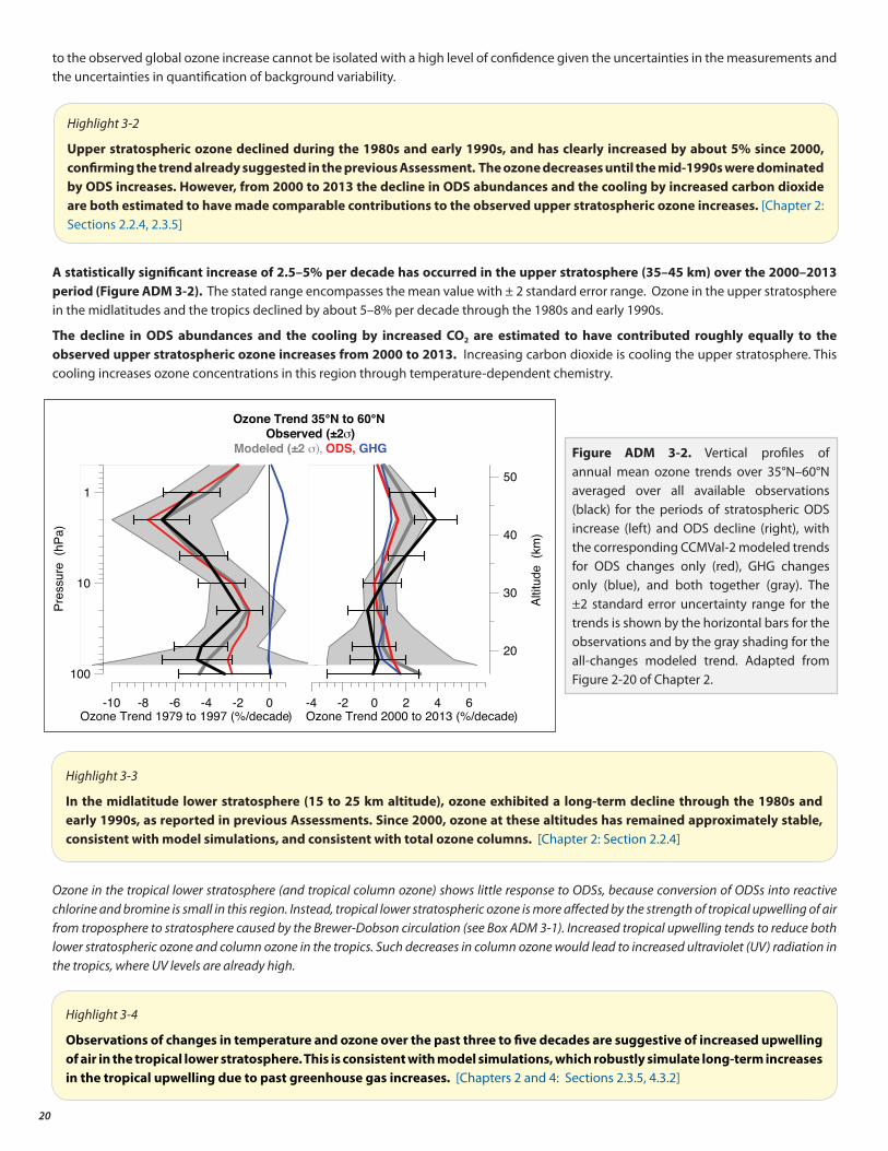
20
to the observed global ozone increase cannot be isolated with a high level of confidence given the uncertainties in the measurements and the uncertainties in quantification of background variability.
A statistically significant increase of 2.5–5% per decade has occurred in the upper stratosphere (35–45 km) over the 2000–2013 period (Figure ADM 3-2). The stated range encompasses the mean value with ± 2 standard error range. Ozone in the upper stratosphere in the midlatitudes and the tropics declined by about 5–8% per decade through the 1980s and early 1990s.
The decline in ODS abundances and the cooling by increased CO2 are estimated to have contributed roughly equally to the observed upper stratospheric ozone increases from 2000 to 2013. Increasing carbon dioxide is cooling the upper stratosphere. This cooling increases ozone concentrations in this region through temperature-dependent chemistry.
Ozone in the tropical lower stratosphere (and tropical column ozone) shows little response to ODSs, because conversion of ODSs into reactive chlorine and bromine is small in this region. Instead, tropical lower stratospheric ozone is more affected by the strength of tropical upwelling of air from troposphere to stratosphere caused by the Brewer-Dobson circulation (see Box ADM 3-1). Increased tropical upwelling tends to reduce both lower stratospheric ozone and column ozone in the tropics. Such decreases in column ozone would lead to increased ultraviolet (UV) radiation in the tropics, where UV levels are already high.
Highlight 3-3
In the midlatitude lower stratosphere (15 to 25 km altitude), ozone exhibited a long-term decline through the 1980s and early 1990s, as reported in previous Assessments. Since 2000, ozone at these altitudes has remained approximately stable, consistent with model simulations, and consistent with total ozone columns. [Chapter 2: Section 2.2.4]
Highlight 3-2
Upper stratospheric ozone declined during the 1980s and early 1990s, and has clearly increased by about 5% since 2000, confirming the trend already suggested in the previous Assessment. The ozone decreases until the mid-1990s were dominated by ODS increases. However, from 2000 to 2013 the decline in ODS abundances and the cooling by increased carbon dioxide are both estimated to have made comparable contributions to the observed upper stratospheric ozone increases. [Chapter 2: Sections 2.2.4, 2.3.5]
-4 -2 0 2 4 6Ozone Trend 2000 to 2013 (%/decade )
100
10
1
-10 -8 -6 -4 -2 0Ozone Trend 1979 to 1997 (%/decade )
20
30
40
50
Ozone Trend 35°N to 60°N Observed (±2σ)
Modeled (±2 σ), ODS, GHG
Pres
sure
(hP
a)
Altit
ude
(km
)
Figure ADM 3-2. Vertical profiles of annual mean ozone trends over 35°N–60°N averaged over all available observations (black) for the periods of stratospheric ODS increase (left) and ODS decline (right), with the corresponding CCMVal-2 modeled trends for ODS changes only (red), GHG changes only (blue), and both together (gray). The ±2 standard error uncertainty range for the trends is shown by the horizontal bars for the observations and by the gray shading for the all-changes modeled trend. Adapted from Figure 2-20 of Chapter 2.
Highlight 3-4
Observations of changes in temperature and ozone over the past three to five decades are suggestive of increased upwelling of air in the tropical lower stratosphere. This is consistent with model simulations, which robustly simulate long-term increases in the tropical upwelling due to past greenhouse gas increases. [Chapters 2 and 4: Sections 2.3.5, 4.3.2]
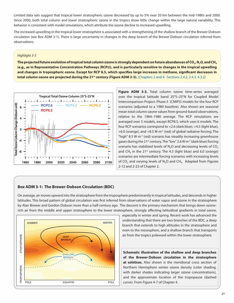
21
Limited data sets suggest that tropical lower stratospheric ozone decreased by up to 5% near 20 km between the mid-1980s and 2000. Since 2000, both total column and lower stratospheric ozone in the tropics show little change within the large natural variability. This behavior is consistent with model simulations, which attribute the ozone decline to increased upwelling.
The increased upwelling in the tropical lower stratosphere is associated with a strengthening of the shallow branch of the Brewer-Dobson circulation (see Box ADM 3-1). There is large uncertainty in changes in the deep branch of the Brewer-Dobson circulation inferred from observations.
Highlight 3-5
The projected future evolution of tropical total column ozone is strongly dependent on future abundances of CO2, N2O, and CH4 (e.g., as in Representative Concentration Pathways (RCPs)), and is particularly sensitive to changes in the tropical upwelling and changes in tropospheric ozone. Except for RCP 8.5, which specifies large increases in methane, significant decreases in total column ozone are projected during the 21st century (Figure ADM 3-3). [Chapters 2 and 4: Sections 2.4.2, 2.4.3, 4.3.2]
Tropical Total Ozone Column 25°S-25°N
Tota
l Ozo
ne C
olum
n Ch
ange
(Dob
son
unit)
Figure ADM 3-3. Total column ozone time-series averaged over the tropical latitude band 25°S–25°N for Coupled Model Intercomparison Project–Phase 5 (CMIP5) models for the four RCP scenarios (adjusted to a 1980 baseline). Also shown are seasonal mean total column ozone values from ground-based observations, relative to the 1964–1980 average. The RCP simulations are averaged over 5 models, except RCP8.5, which uses 6 models. The four RCP scenarios correspond to +2.6 (dark blue), +4.5 (light blue), +6.0 (orange), and +8.5 W m-2 (red) of global radiative forcing. The "high" 8.5 W m-2 (red) scenario has steadily increasing greenhouse gases during the 21st century. The "low" 2.6 W m-2 (dark blue) forcing scenario has stabilized levels of N2O and decreasing levels of CO2 and CH4 in the 21st century. The 4.5 (light blue) and 6.0 (orange) scenarios are intermediate forcing scenarios with increasing levels of CO2 and varying levels of N2O and CH4. Adapted from Figures 2-12 and 2-23 of Chapter 2.
Box ADM 3-1: The Brewer-Dobson Circulation (BDC)
On average, air moves upward into the stratosphere from the troposphere predominantly in tropical latitudes, and descends in higher latitudes. This broad pattern of global circulation was first inferred from observations of water vapor and ozone in the stratosphere by Alan Brewer and Gordon Dobson more than a half-century ago. The descent is the primary mechanism that brings down ozone-rich air from the middle and upper stratosphere to the lower stratosphere, strongly affecting latitudinal gradients in total ozone,
especially in winter and spring. Recent work has advanced the understanding that there are two branches of the BDC, a deep branch that extends to high altitudes in the stratosphere and even to the mesosphere, and a shallow branch that transports air from the tropics poleward within the lower stratosphere.
EQUATOR POLEPOLETRO
POSP
HER
EST
RAT
OSP
HER
E
DEEPBRANCH
SHALLOWBRANCH
SUMMER WINTER
Schematic illustration of the shallow and deep branches of the Brewer-Dobson circulation in the stratosphere at solstices. Also shown is the meridional cross section of Northern Hemisphere winter ozone density (color shading, with darker shades indicating larger ozone concentrations), and the approximate location of the tropopause (dashed curve). From Figure 4-7 of Chapter 4.

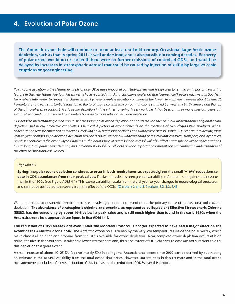
23
Polar ozone depletion is the clearest example of how ODSs have impacted our stratosphere, and is expected to remain an important, recurring feature in the near future. Previous Assessments have reported that Antarctic ozone depletion (the “ozone hole”) occurs each year in Southern Hemisphere late winter to spring. It is characterized by near-complete depletion of ozone in the lower stratosphere, between about 12 and 20 kilometers, and a very substantial reduction in the total ozone column (the amount of ozone summed between the Earth surface and the top of the atmosphere). In contrast, Arctic ozone depletion in late winter to spring is very variable. It has been small in many previous years but stratospheric conditions in some Arctic winters have led to more substantial ozone depletion.
Our detailed understanding of the annual winter-spring polar ozone depletion has bolstered confidence in our understanding of global ozone depletion and in our predictive capabilities. Chemical depletion of ozone depends on the reactions of ODS degradation products, whose concentrations can be enhanced by reactions involving polar stratospheric clouds and sulfuric acid aerosol. While ODSs continue to decline, large year-to-year changes in polar ozone depletion provide a critical test of our understanding of the relevant chemical, transport, and dynamical processes controlling the ozone layer. Changes in the abundance of stratospheric aerosol will also affect stratospheric ozone concentrations. Future long-term polar ozone changes, and interannual variability, will both provide important constraints on our continuing understanding of the effects of the Montreal Protocol.
Well understood stratospheric chemical processes involving chlorine and bromine are the primary cause of the seasonal polar ozone depletion. The abundance of stratospheric chlorine and bromine, as represented by Equivalent Effective Stratospheric Chlorine (EESC), has decreased only by about 10% below its peak value and is still much higher than found in the early 1980s when the Antarctic ozone hole appeared (see figure in Box ADM 1-1).
The reduction of ODSs already achieved under the Montreal Protocol is not yet expected to have had a major effect on the extent of the Antarctic ozone hole. The Antarctic ozone hole is driven by the very low temperatures inside the polar vortex, which make almost all chlorine and bromine from the ODSs available for ozone depletion. Near-complete ozone depletion occurs at high polar latitudes in the Southern Hemisphere lower stratosphere and, thus, the extent of ODS changes to date are not sufficient to alter this depletion to a great extent.
A small increase of about 10–25 DU (approximately 5%) in springtime Antarctic total ozone since 2000 can be derived by subtracting an estimate of the natural variability from the total ozone time series. However, uncertainties in this estimate and in the total ozone measurements preclude definitive attribution of this increase to the reduction of ODSs over this period.
The Antarctic ozone hole will continue to occur at least until mid-century. Occasional large Arctic ozone depletion, such as that in spring 2011, is well understood, and is also possible in coming decades. Recovery of polar ozone would occur earlier if there were no further emissions of controlled ODSs, and would be delayed by increases in stratospheric aerosol that could be caused by injection of sulfur by large volcanic eruptions or geoengineering.
4. Evolution of Polar Ozone
Highlight 4-1
Springtime polar ozone depletion continues to occur in both hemispheres, as expected given the small (~10%) reductions to date in ODS abundances from their peak values. The last decade has seen greater variability in Antarctic springtime polar ozone than in the 1990s (see Figure ADM 4-1). This ozone variability results from natural year-to-year changes in meteorological processes and cannot be attributed to recovery from the effect of the ODSs. [Chapters 2 and 3: Sections 2.2, 3.2, 3.4]
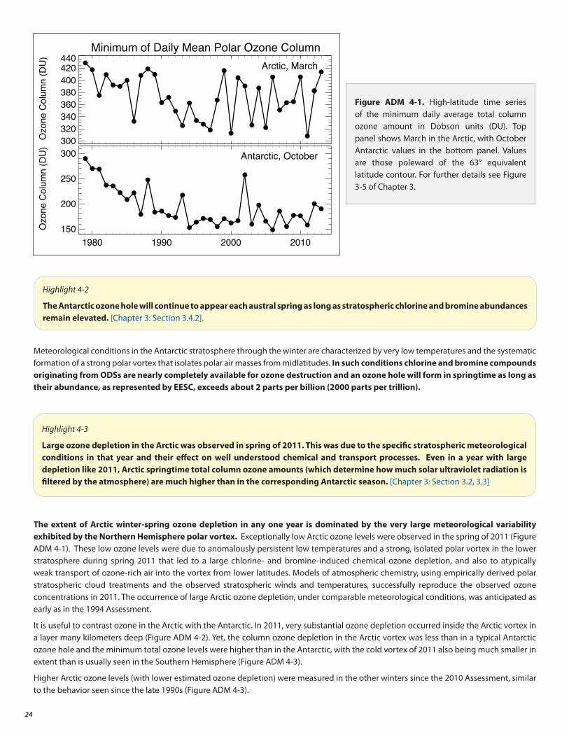
24
Meteorological conditions in the Antarctic stratosphere through the winter are characterized by very low temperatures and the systematic formation of a strong polar vortex that isolates polar air masses from midlatitudes. In such conditions chlorine and bromine compounds originating from ODSs are nearly completely available for ozone destruction and an ozone hole will form in springtime as long as their abundance, as represented by EESC, exceeds about 2 parts per billion (2000 parts per trillion).
The extent of Arctic winter-spring ozone depletion in any one year is dominated by the very large meteorological variability exhibited by the Northern Hemisphere polar vortex. Exceptionally low Arctic ozone levels were observed in the spring of 2011 (Figure ADM 4-1). These low ozone levels were due to anomalously persistent low temperatures and a strong, isolated polar vortex in the lower stratosphere during spring 2011 that led to a large chlorine- and bromine-induced chemical ozone depletion, and also to atypically weak transport of ozone-rich air into the vortex from lower latitudes. Models of atmospheric chemistry, using empirically derived polar stratospheric cloud treatments and the observed stratospheric winds and temperatures, successfully reproduce the observed ozone concentrations in 2011. The occurrence of large Arctic ozone depletion, under comparable meteorological conditions, was anticipated as early as in the 1994 Assessment.
It is useful to contrast ozone in the Arctic with the Antarctic. In 2011, very substantial ozone depletion occurred inside the Arctic vortex in a layer many kilometers deep (Figure ADM 4-2). Yet, the column ozone depletion in the Arctic vortex was less than in a typical Antarctic ozone hole and the minimum total ozone levels were higher than in the Antarctic, with the cold vortex of 2011 also being much smaller in extent than is usually seen in the Southern Hemisphere (Figure ADM 4-3).
Higher Arctic ozone levels (with lower estimated ozone depletion) were measured in the other winters since the 2010 Assessment, similar to the behavior seen since the late 1990s (Figure ADM 4-3).
Highlight 4-3
Large ozone depletion in the Arctic was observed in spring of 2011. This was due to the specific stratospheric meteorological conditions in that year and their effect on well understood chemical and transport processes. Even in a year with large depletion like 2011, Arctic springtime total column ozone amounts (which determine how much solar ultraviolet radiation is filtered by the atmosphere) are much higher than in the corresponding Antarctic season. [Chapter 3: Section 3.2, 3.3]
Minimum of Daily Mean Polar Ozone Column
300320340360380400420440
Ozo
ne C
olum
n (D
U)
Arctic, March
1980 1990 2000 2010150
200
250
300
Ozo
ne C
olum
n (D
U)
Antarctic, October
Figure ADM 4-1. High-latitude time series of the minimum daily average total column ozone amount in Dobson units (DU). Top panel shows March in the Arctic, with October Antarctic values in the bottom panel. Values are those poleward of the 63° equivalent latitude contour. For further details see Figure 3-5 of Chapter 3.
Highlight 4-2
The Antarctic ozone hole will continue to appear each austral spring as long as stratospheric chlorine and bromine abundances remain elevated. [Chapter 3: Section 3.4.2].
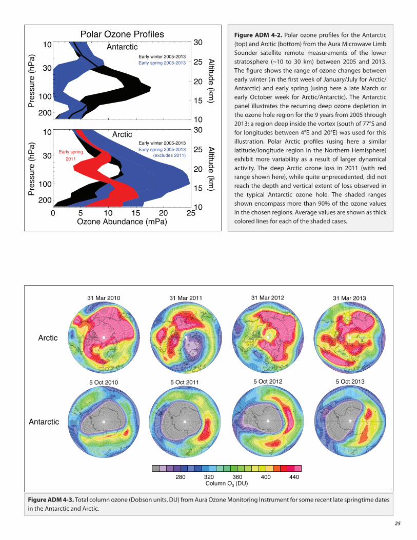
25
30
30
200
200
Polar Ozone Profiles
100
10Pr
essu
re (h
Pa)
10
15
20
25
30
Altitude (km)
Antarctic
0 5 10 15 20 25Ozone Abundance (mPa)
100
10
Pres
sure
(hPa
)
10
15
20
25
30
Altitude (km)
Arctic
Early winter 2005-2013Early spring 2005-2013
Early winter 2005-2013Early spring 2005-2013
(excludes 2011)Early spring
2011
Figure ADM 4-2. Polar ozone profiles for the Antarctic (top) and Arctic (bottom) from the Aura Microwave Limb Sounder satellite remote measurements of the lower stratosphere (~10 to 30 km) between 2005 and 2013. The figure shows the range of ozone changes between early winter (in the first week of January/July for Arctic/Antarctic) and early spring (using here a late March or early October week for Arctic/Antarctic). The Antarctic panel illustrates the recurring deep ozone depletion in the ozone hole region for the 9 years from 2005 through 2013; a region deep inside the vortex (south of 77°S and for longitudes between 4°E and 20°E) was used for this illustration. Polar Arctic profiles (using here a similar latitude/longitude region in the Northern Hemisphere) exhibit more variability as a result of larger dynamical activity. The deep Arctic ozone loss in 2011 (with red range shown here), while quite unprecedented, did not reach the depth and vertical extent of loss observed in the typical Antarctic ozone hole. The shaded ranges shown encompass more than 90% of the ozone values in the chosen regions. Average values are shown as thick colored lines for each of the shaded cases.
5 Oct 2010
Antarctic
5 Oct 2011 5 Oct 2012 5 Oct 2013
31 Mar 2010
Arctic
31 Mar 2011
31 Mar 2012
31 Mar 2013
280 320 360 400 440Column O3 (DU)
Figure ADM 4-3. Total column ozone (Dobson units, DU) from Aura Ozone Monitoring Instrument for some recent late springtime dates in the Antarctic and Arctic.
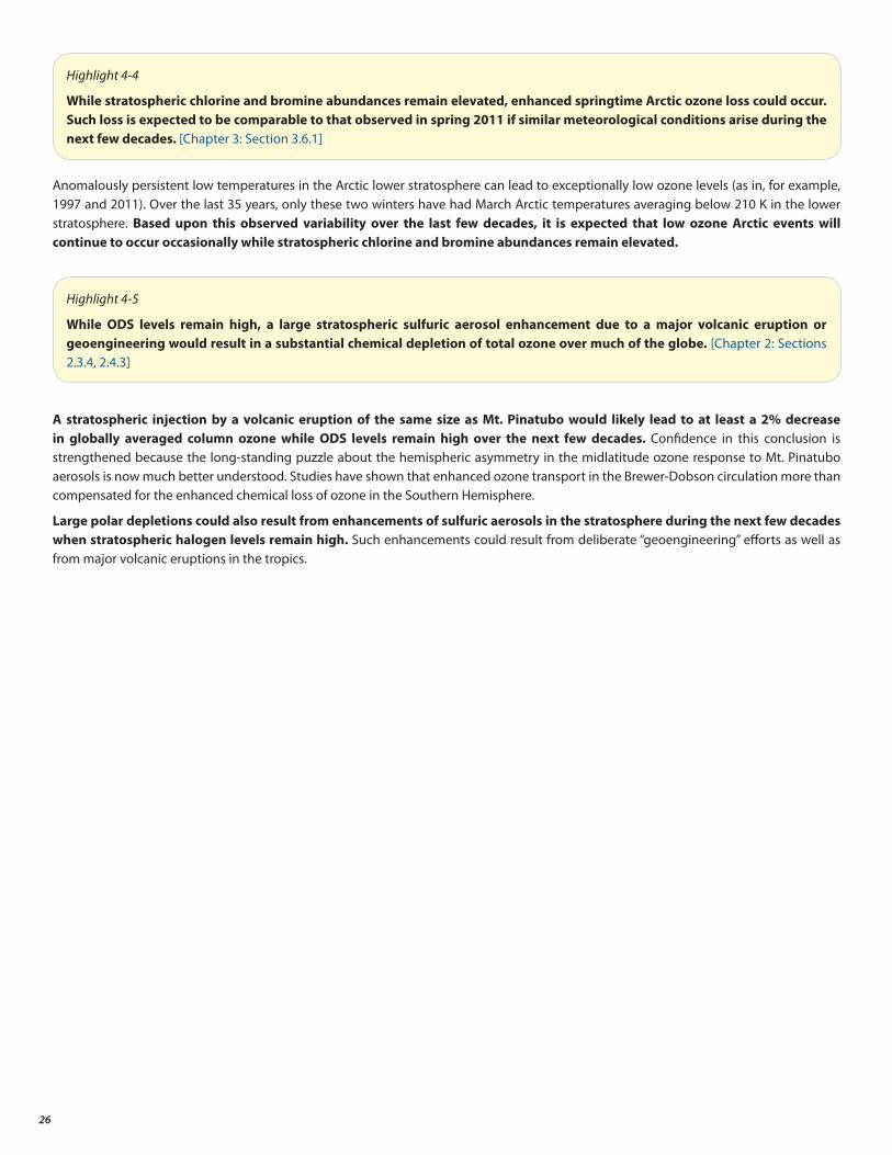
26
Anomalously persistent low temperatures in the Arctic lower stratosphere can lead to exceptionally low ozone levels (as in, for example, 1997 and 2011). Over the last 35 years, only these two winters have had March Arctic temperatures averaging below 210 K in the lower stratosphere. Based upon this observed variability over the last few decades, it is expected that low ozone Arctic events will continue to occur occasionally while stratospheric chlorine and bromine abundances remain elevated.
A stratospheric injection by a volcanic eruption of the same size as Mt. Pinatubo would likely lead to at least a 2% decrease in globally averaged column ozone while ODS levels remain high over the next few decades. Confidence in this conclusion is strengthened because the long-standing puzzle about the hemispheric asymmetry in the midlatitude ozone response to Mt. Pinatubo aerosols is now much better understood. Studies have shown that enhanced ozone transport in the Brewer-Dobson circulation more than compensated for the enhanced chemical loss of ozone in the Southern Hemisphere.
Large polar depletions could also result from enhancements of sulfuric aerosols in the stratosphere during the next few decades when stratospheric halogen levels remain high. Such enhancements could result from deliberate “geoengineering” efforts as well as from major volcanic eruptions in the tropics.
Highlight 4-5
While ODS levels remain high, a large stratospheric sulfuric aerosol enhancement due to a major volcanic eruption or geoengineering would result in a substantial chemical depletion of total ozone over much of the globe. [Chapter 2: Sections 2.3.4, 2.4.3]
Highlight 4-4
While stratospheric chlorine and bromine abundances remain elevated, enhanced springtime Arctic ozone loss could occur. Such loss is expected to be comparable to that observed in spring 2011 if similar meteorological conditions arise during the next few decades. [Chapter 3: Section 3.6.1]
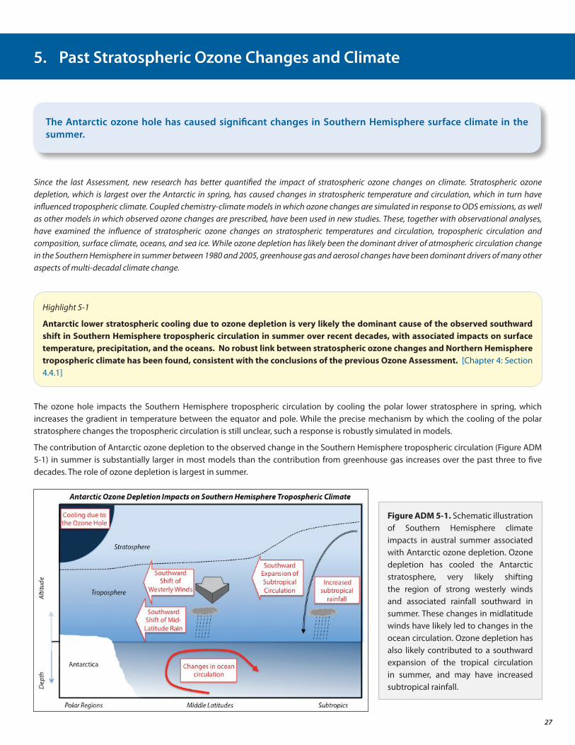
27
Since the last Assessment, new research has better quantified the impact of stratospheric ozone changes on climate. Stratospheric ozone depletion, which is largest over the Antarctic in spring, has caused changes in stratospheric temperature and circulation, which in turn have influenced tropospheric climate. Coupled chemistry-climate models in which ozone changes are simulated in response to ODS emissions, as well as other models in which observed ozone changes are prescribed, have been used in new studies. These, together with observational analyses, have examined the influence of stratospheric ozone changes on stratospheric temperatures and circulation, tropospheric circulation and composition, surface climate, oceans, and sea ice. While ozone depletion has likely been the dominant driver of atmospheric circulation change in the Southern Hemisphere in summer between 1980 and 2005, greenhouse gas and aerosol changes have been dominant drivers of many other aspects of multi-decadal climate change.
The ozone hole impacts the Southern Hemisphere tropospheric circulation by cooling the polar lower stratosphere in spring, which increases the gradient in temperature between the equator and pole. While the precise mechanism by which the cooling of the polar stratosphere changes the tropospheric circulation is still unclear, such a response is robustly simulated in models.
The contribution of Antarctic ozone depletion to the observed change in the Southern Hemisphere tropospheric circulation (Figure ADM 5-1) in summer is substantially larger in most models than the contribution from greenhouse gas increases over the past three to five decades. The role of ozone depletion is largest in summer.
The Antarctic ozone hole has caused significant changes in Southern Hemisphere surface climate in the summer.
5. Past Stratospheric Ozone Changes and Climate
Highlight 5-1
Antarctic lower stratospheric cooling due to ozone depletion is very likely the dominant cause of the observed southward shift in Southern Hemisphere tropospheric circulation in summer over recent decades, with associated impacts on surface temperature, precipitation, and the oceans. No robust link between stratospheric ozone changes and Northern Hemisphere tropospheric climate has been found, consistent with the conclusions of the previous Ozone Assessment. [Chapter 4: Section 4.4.1]
Figure ADM 5-1. Schematic illustration of Southern Hemisphere climate impacts in austral summer associated with Antarctic ozone depletion. Ozone depletion has cooled the Antarctic stratosphere, very likely shifting the region of strong westerly winds and associated rainfall southward in summer. These changes in midlatitude winds have likely led to changes in the ocean circulation. Ozone depletion has also likely contributed to a southward expansion of the tropical circulation in summer, and may have increased subtropical rainfall.
28
Climate models simulate a southward shift of the Southern Hemisphere midlatitude maximum in precipitation in austral summer in response to stratospheric ozone depletion. There is some evidence of a consistent pattern of rainfall trends in observations.
In the Southern Hemisphere summer, stratospheric ozone depletion has likely contributed to a southward expansion of the tropical circulation, which influences precipitation in subtropical regions (Figure ADM 5-1).
Observational and modeling studies present a broadly consistent picture of the ocean’s response to surface wind stress changes, which have likely been substantially caused by stratospheric ozone changes. This involves intensification of the subtropical ocean gyres and the north-south overturning circulations, with an accompanying subsurface warming. The impact of these wind stress changes on ocean carbon uptake from the atmosphere remains uncertain.
The influence of stratospheric ozone depletion on Antarctic sea ice increases reported in the last Ozone Assessment is not supported by a number of new coupled-model studies. These suggest that ozone depletion causes a decrease in Southern Hemisphere sea ice extent and thus did not lead to the small observed increase. However, there is low confidence in this model result because of large uncertainties in the simulation of Antarctic sea ice.
Ozone recovery is expected to drive a weakening and equatorward shift of the summertime Southern Hemisphere midlatitude jet, while increases in greenhouse gases are expected to drive a strengthening and poleward shift of the jet. Under a low greenhouse gas emissions scenario, ozone recovery is expected to dominate the effect of greenhouse gas increases on Southern Hemisphere tropospheric circulation in austral summer to give a weakening and equatorward shift of the midlatitude jet over the next 50 years, while in a high greenhouse gas emissions scenario the jet is projected to continue to shift poleward and to strengthen.
Highlight 5-2
There is further evidence that in austral summer, Antarctic stratospheric ozone recovery and increases in greenhouse gases will have opposite effects on the Southern Hemisphere tropospheric circulation, with associated impacts on surface temperature, precipitation, and the oceans. [Chapter 4: Section 4.5.1]
29
Ozone-layer depletion is caused by chemical reactions with chlorine and bromine compounds released from anthropogenic ODSs in the stratosphere. As noted in Figure ADM 1-3, ODSs are declining in our atmosphere and are projected to decline into the future. In response to this ODS decline, global ozone levels have stabilized (see ADM Highlights, Section 3) and will increase, and global ozone amounts will return to 1980 levels during the 21st century (see Figure ADM 6-2, bottom panel).
The primary greenhouse gases (GHGs) are CO2 , N2O, and CH4 . In the last Assessment, it was noted that increasing levels of these GHGs warm the troposphere and cool the stratosphere. This stratospheric cooling modifies the rates of some chemical reactions, generally lessening ozone loss rates, and thereby increasing ozone levels. Hence, future ozone levels will increase beyond levels observed prior to 1960. In addition to modifying stratospheric temperatures, N2O and CH4 alter the chemistry of the stratosphere by degrading into reactive nitrogen and hydrogen compounds. The reactive nitrogen compounds from the additional N2O mainly deplete ozone, while the reactive hydrogen compounds from CH4 increase ozone by mitigating chlorine-driven ozone depletion.
Future levels of GHGs will modify the stratosphere, but projecting how CO2 , N2O, and CH4 will change in the future is very difficult because of changing economics, government policies, and feedback factors in the Earth system. Four possible greenhouse gas (CO2 , CH4 , and N2O) projections have been developed for IPCC. These four GHG projections are radiative forcing outcomes that correspond to +2.6, +4.5, +6.0, and +8.5 W m-2 of global radiative forcing by the year 2100. The “high” 8.5 W m-2 scenario has steadily increasing CO2 , CH4 , and N2O over the course of the 21st century. The “low” 2.6 W m-2 forcing scenario has stabilized levels of N2O and decreasing levels of CO2 and CH4 in the 21st century. The 4.5 and 6.0 W m-2 scenarios are intermediate global radiative forcings with increasing levels of CO2 and varying levels of N2O and CH4.
Between 1979 and 1995, the global mean lower stratospheric temperature decreased by about 1°C but has since remained approximately constant, consistent with the approximately constant ozone abundance. Greenhouse gas increases have only had a minor contribution to cooling in this region, with volcanic aerosols driving episodic warming.
The observed cooling of the Antarctic lower stratosphere since 1979 during austral spring is consistent with the average simulated cooling in models forced by observed ozone variations. There is a large range in the magnitude of the simulated cooling: chemistry-climate models that underestimate the ozone depletion also underestimate the cooling.
In the middle and upper stratosphere, observed globally averaged temperatures decreased from 1979 to 2005, but the magnitude of the cooling is uncertain. While observations of upper stratospheric temperatures have continued since 2005 and indicate further cooling, there is currently no global satellite temperature record available for the upper stratosphere that would be homogeneous over the entire 1979 to 2013 period.
Ozone-depleting substances (ODSs) were the dominant driver of global ozone decline in the late 20th century. As controlled ODS concentrations decline, carbon dioxide (CO2), nitrous oxide (N2O), and methane (CH4) will strongly influence ozone evolution in the latter part of the 21st century through chemical and climate effects. N2O increases will tend to decrease ozone, while increasing CH4 and CO2 will tend to increase ozone. Uncertainties in future emissions of these gases lead to large differences in ozone projections at the end of the century.
6. The Future of the Ozone Layer
Highlight 6-1
In the lower stratosphere, ozone depletion has been the dominant cause of the observed globally averaged long-term cooling since about 1980. In the upper stratosphere, models indicate that increasing greenhouse gases and ozone changes have made comparable contributions to the observed cooling. [Chapter 4: Section 4.3.1]

30
As shown in Figure ADM 6-1, global ozone (magenta points) has declined, but future ozone levels (black line) will steadily increase. CO2 increases alone (red line) lead to increasing global ozone levels. Higher N2O alone (green line) reduces column ozone, while higher CH4 alone (brown line) increases column ozone, each by a few percent from 2020 to 2100, with the magnitude of these effects on ozone being comparable to what is expected from stratospheric cooling by CO2 increases. The influence of each individual trace gas (CO2, N2O, or CH4) on ozone also depends on projections of the other gases, so that their combined impact on ozone is strongly scenario dependent (see Figure ADM 6-2).
The combined effects of future increased CO2, N2O, and CH4 levels could bring forward the recovery of ozone by two to four decades.
Models that include chemistry, climate, and ocean processes interactively show differing amounts of ozone changes for various Representative Concentration Pathway (RCP) greenhouse gas scenarios. Figure ADM 6-2 shows how global ozone responds to these future RCP greenhouse gas scenarios. The 8.5 W m-2 “high” radiative forcing scenario (red) shows a 6% increase above 1960–1980 ozone levels by 2100, whereas the 2.6 W m-2 “low” scenario (magenta) shows a change of about 0% with respect to the 1960–1980 ozone level. These projected total ozone columns in 2100 differ by up to 20 DU in the global average. This range of change is comparable to the depletion caused to date by ODSs (see Figure ADM 6-2).
Part of the considerable scenario uncertainty in future column ozone is due to differences in emissions of N2O and CH4 between the various RCP scenarios. We do not have much confidence in our understanding of the current budgets of N2O and CH4 and explaining the recent changes in their atmospheric growth rate is a current scientific challenge; projections of their concentrations in the future are, therefore, uncertain.
Highlight 6-2
The evolution of the ozone layer in the late 21st century will largely depend on the atmospheric abundances of CO2 , N2O, and CH4. Increases of CO2 , and to a lesser extent N2O and CH4 , will cool the stratosphere radiatively, elevating global ozone. The major impact on ozone of N2O and CH4 is due to chemical processes. Increasing N2O will drive global ozone depletion, whereas rising CH4 levels drive column ozone increases (see Figure ADM 6-1). [Chapters 2 and 3: Sections 2.4, 3.5]
Global Total Ozone
10
0
-10
-20
4
-4
0 % C
hange
ODS only
Base
N2O only
CH4 only
CO2 only
Tota
l Ozo
ne C
hang
e (D
U)
1960 2000 2040 2080
2
-2
-6
Figure ADM 6-1. Model-simulated global/annual averaged total ozone response to the changes in CO2 (red line), CH4 (brown line), N2O (green line), and ODSs (blue line). The total response to ODSs and GHGs combined is shown as the black line. The responses are taken relative to 1960 values. Future GHG concentrations are based on the IPCC SRES A1B (medium) scenario. Ground-based total ozone observations (base-lined to the mid-1960s) are shown as magenta cross symbols. Adapted from Figure 2-24 of Chapter 2.
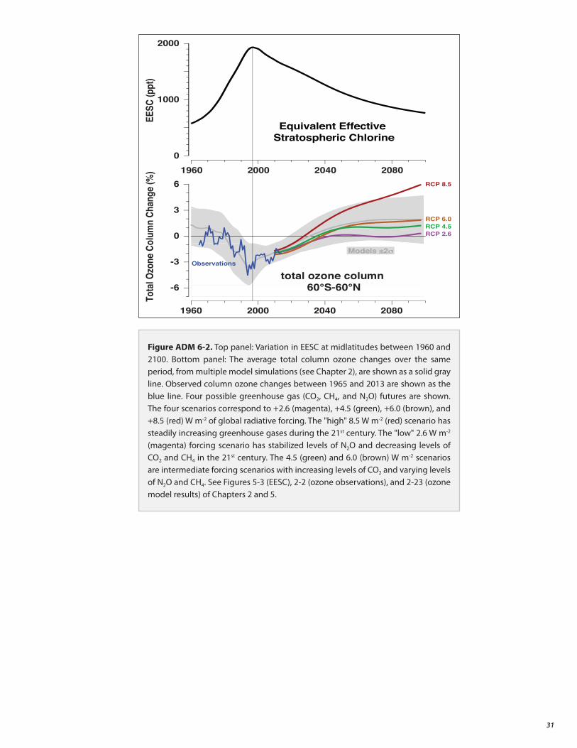
31
0
1000
2000
EESC
(ppt
)
Equivalent Effective Stratospheric Chlorine
-6
-3
0
3
6
Tota
l Ozo
ne C
olum
n Ch
ange
(%)
Models ±2σ
RCP 8.5
RCP 6.0RCP 4.5RCP 2.6
total ozone column 60°S-60°N
2080204020001960
2080204020001960
Observations
Figure ADM 6-2. Top panel: Variation in EESC at midlatitudes between 1960 and 2100. Bottom panel: The average total column ozone changes over the same period, from multiple model simulations (see Chapter 2), are shown as a solid gray line. Observed column ozone changes between 1965 and 2013 are shown as the blue line. Four possible greenhouse gas (CO2, CH4, and N2O) futures are shown. The four scenarios correspond to +2.6 (magenta), +4.5 (green), +6.0 (brown), and +8.5 (red) W m-2 of global radiative forcing. The "high" 8.5 W m-2 (red) scenario has steadily increasing greenhouse gases during the 21st century. The "low" 2.6 W m-2 (magenta) forcing scenario has stabilized levels of N2O and decreasing levels of CO2 and CH4 in the 21st century. The 4.5 (green) and 6.0 (brown) W m-2 scenarios are intermediate forcing scenarios with increasing levels of CO2 and varying levels of N2O and CH4. See Figures 5-3 (EESC), 2-2 (ozone observations), and 2-23 (ozone model results) of Chapters 2 and 5.

33
ADDITIONAL INFORMATIONOF INTEREST TO DECISION-MAKERS
• Metrics for Changes in Ozone and Climate
• Scenarios and Sensitivity Analyses

35
[Excerpted and adapted with slight modifications from Chapter 5 of the 2014 report of the Scientific Assessment Panel of the Montreal Protocol, “Scientific Assessment of Ozone Depletion: 2014.” For references, tables, figures, and chapter sections mentioned in this excerpt, please refer to Chapter 5, available online at: http://ozone.unep.org/en/assessment_panels_bodies.php?committee_id=7 or http://www.wmo.int/pages/prog/arep/gaw/ozone_2014/ozone_asst_report.html]
For the purpose of this Assessment, metrics are defined as tools used for quantifying and comparing impacts of emissions from human activity. Typically they aggregate and simplify complex information about different substances, placing them on a common scale to enable comparison of impacts. Metrics such as Equivalent Effective Stratospheric Chlorine (EESC) and Ozone Depletion Potentials (ODPs) have proven to be important tools in policy considerations for addressing stratospheric ozone-layer depletion, while other metrics, including radiative forcing (RF) and Global Warming Potentials (GWPs), have proven to be useful tools in climate policy. These metrics have all been used in past Assessments of ozone and climate including the WMO Assessments. In addition, newer metrics, such as Global Temperature change Potentials (GTPs), are introduced in the discussion below.
Some of these metrics express the integrated impact of a given substance relative to that for the release of the same mass of a reference compound (generally CFC-11 for ODPs and CO2 for GWPs and GTPs). For such metrics that use relative indices, some uncertainties in translating emissions into absolute environmental impacts tend to cancel, and the relative benefits of controlling emissions of different substances are highlighted. However, it should be recognized that the metrics discussed here do not represent the full complexity of the chemistry and physics of the atmosphere (e.g., where and when the ozone depletion occurs). Though simple, some caution is required when interpreting the values derived (e.g., how much are these values dependent on the background atmosphere assumed in their derivation). ODPs and GWPs have found widespread use in national regulatory actions and in international agreements such as the Montreal Protocol and the Kyoto Protocol.
5.3.1 Metrics for changes in ozone
Metrics for Changes in Ozone and Climate
Metrics for Ozone: The Basics
Equivalent Effective Stratospheric Chlorine (EESC)EESC is a sum of the time-dependent chlorine and bromine derived from tropospheric abundances of ODSs weighted to reflect their potential influence on ozone. EESC has become a standard benchmark for estimating ozone depletion relative to a base period, usually taken as 1980 (a time before major ozone depletion). EESC relates surface mixing ratios of chlorine- and bromine-containing ODSs to the stratospheric inorganic chlorine and bromine released from these substances in key regions of the stratosphere and thus to the amount of ozone they will destroy (Daniel et al., 1995; WMO, 1995, 1999, 2003, 2007, 2011; also see Chapter 1). EESC also accounts for the larger efficiency of bromine to destroy stratospheric ozone compared to chlorine (on a per-atom basis) and differences in where in the stratosphere the ODSs release their chlorine and bromine. EESC has been reformulated (Newman et al., 2007) to account for the spread in the time it takes tropospheric air to get to a given location in the stratosphere, the so-called “age-of-air spectrum,” and the age-of-air dependent fractional release values. Not only does this increase its accuracy, but EESC can also then be derived for various latitudes, including effects at midlatitudes or in the Antarctic vortex (Newman et al., 2009; WMO, 2011). The changes in integrated EESC and the date when EESC returns to 1980 levels have both been used in the previous WMO Assessments to quantify the relative impacts of future emissions of ODSs. In Section 5.4, EESC is used in the evaluation of scenarios for various assumptions about future emissions of halocarbons. The EESC concept has been further revised (Daniel et al., 2010) to account for the effects of nitrous oxide (N2O), the primary source for nitrogen oxides (NOx = NO + NO2 ) in the stratosphere.
EESC is calculated as in previous Assessments. The only difference between the calculations in the 2010 Ozone Assessment (WMO, 2011) and those here is that we now use an age spectrum for both midlatitude (3-year mean age) and Antarctic conditions (5.5-year mean age), while a full age spectrum was not used before. In both cases, we assume the width of the spectrum is equal to half of the average age (Newman et al., 2007). A complete discussion of the other aspects of the EESC calculation can be found in Chapter 5 of WMO (2011). As in that Assessment, we assume the relative impact of bromine compared to chlorine for ozone destruction, typically referred to as α, is 60 at midlatitudes and 65 in polar regions.
Ozone Depletion Potentials (ODPs)The concept of Ozone Depletion Potentials (ODPs) (Wuebbles 1981, 1983; Solomon et al. 1992; the various WMO Assessments) arose as a means of determining the relative ability of a chemical to destroy ozone. Steady-state ODPs are defined as the change in global
36
Updating the Evaluation of ODPs
There have been only a few published updates on ODP values since the last Assessment, with most of those concerning VSLS as discussed below. Papanastasiou et al. (2013) provide analyses of updated semi-empirical ODPs for several bromine-containing compounds (halon-1202, -1211, and -2402) using updated lifetimes computed with the NASA Goddard Space Flight Center (GSFC) 2-D atmospheric model (Fleming et al., 2011). Their analyses produced somewhat different ODP values compared to WMO (2011): 1.95 for halon-1202 vs. 1.7 in WMO (2011), 8.1 for halon-1211 vs. 7.9 in WMO (2011), and 18.4 for halon-2402 vs. 13.0 in WMO (2011).
New scientific results affect the earlier ODPs, especially from the reanalysis of atmospheric lifetimes in SPARC (2013). The revised SPARC (2013) recommended lifetimes are based on calculations with atmospheric chemical transport models, analysis of observations at the surface and in the stratosphere, laboratory analysis of chemical reactions and photolysis rates, and inverse modeling. In addition, the SPARC report provides uncertainties in the lifetimes of major halogenated ODS. The uncertainties in the lifetimes are considerable, ranging from 3% to 33% (one standard deviation, 1σ; also see Velders and Daniel (2014) for further discussion on these uncertainties). The SPARC (2013) atmospheric lifetimes are compared to those from WMO (2011) in Table 5-1 [included as ADM Appendix C of this document] (also see discussion of atmospheric lifetimes in Chapter 1). There are a number of differences, but the most important one to the derivation of ODPs is the change in lifetime of CFC-11 from 45 years to 52 years (+15%); because CFC-11 is in the denominator in ODP derivation, this change in lifetime decreases the values of all ODPs in WMO (2011) by 15%. Revisions in the lifetimes for other substances produce the other differences found in ODP values for “This Assessment” found in Table 5-2 [included as ADM Appendix D of this document].
ozone for a sustained unit mass emission of a specific compound relative to the change in global ozone for the sustained unit mass emission of CFC-11 (CCl3F). This is equivalent to assuming an infinitesimal emission pulse and adding up all the ozone lost until all of the emitted gas is removed from the atmosphere. ODPs provide an important and relatively straightforward way of analyzing the potential for a new chemical to affect ozone relative to the chlorofluorocarbons (CFCs) and other chlorine-, bromine-, and iodine-containing halocarbons. It is also now being applied to non-halogenated compounds like nitrous oxide (N2O) (Ravishankara et al., 2009; Fleming et al., 2011; WMO, 2011) and methane (CH4) (Fleming et al., 2011). ODPs are currently determined by two different means: calculations from chemical transport models (CTMs) of the global atmosphere, and the semi-empirical approach that depends primarily on observations rather than models (Solomon et al., 1992; WMO, 2003, 2007, 2011). Both approaches have been shown to give very similar ODP values in previous Assessments.
Advantages and disadvantages of using ODPs have been discussed in the prior WMO Assessments. Because ODPs are defined relative to the ozone loss caused by CFC-11, it is generally thought that the ODP values demonstrate less sensitivity to photochemical modeling errors than do absolute ozone loss calculations, but this is only strictly true when used for other Cl-containing compounds with similar atmospheric lifetimes. Interpretation of non-halocarbon ODPs could be particularly problematic. For example, ODPs are normally derived relative to the current atmosphere, but there could potentially be some differences in values if they were calculated relative to a future atmosphere with different background composition, temperatures, or circulation.
Originally, the evaluation of ODPs was conducted largely for chemicals with atmospheric lifetimes sufficiently long (> ~1 year) that they are well mixed throughout the troposphere after their emission at the surface, and a significant portion of the surface emissions can still reach the stratosphere. However, many of the compounds being considered either for new applications or as replacements for substances controlled under the Montreal Protocol are now designed to be very short-lived, on the order of days to a few months, so as to reduce the impacts on ozone and climate. Many of these very short-lived substances (VSLS) still contain chlorine, bromine, or iodine, and can be transported vertically into the lower stratosphere particularly through the tropical troposphere. A major complication with VSLS is that the compound can decompose into inorganic halogen compounds in the uppermost tropical troposphere, and chlorine, bromine, and iodine released from the stable gases are still transported, at least partially, to the stratosphere and hence an important uncertainty is the degree to which the inorganic halogens (e.g., HBr, HOBr) are scavenged during the removal of water vapor in ascent. Another issue is that basic assumptions of referencing to CFC-11 to cancel transport and other errors in the model clearly break down since the chemical removal processes are so different; nonetheless there is high value for policymakers in being able to use the modified form of the ODP concept for VSLS.
Due to the difficulties in calculating the dynamical and chemical processes affecting such short-lived compounds, three-dimensional (3-D) models fully representing the troposphere and stratosphere need to be used to predict the halogen loading and resulting effects on global ozone. As a result, the definition of ODPs has been revised for VSLS (Wuebbles et al., 2001; WMO, 2003, 2011; Pisso et al., 2010). The ODPs derived for VSLS now account for variations that can occur in the ODP as a function of where and when (geographic location and time of year) the compound is emitted. The most important factor in evaluating the ODP of VSLS is shown to be geographical distribution, or latitude, of the surface emissions because gases emitted at higher latitudes are less likely to reach the stratosphere before destruction than gases emitted in the tropics (Bridgeman et al., 2000; Olsen et al., 2000; Wuebbles et al., 2001). The discussion of updates to ODPs thus reflects this change in definition for VSLS.
37
The age-of-air spectrum from Newman et al. (2007) and the age-of-air dependent fractional release factors (FRFs, defined as age of-air-dependent ODS decomposition rates; also see Chapter 1) from Newman et al. (2006) were used in WMO (2011) for discrete ages-of-air for midlatitude (3 year) and Antarctic (5.5 year) conditions. A new analysis of the fractional release factor (FRF) for ten ODSs by Laube et al. (2013) gives values that are on average about 20% smaller than those derived by Newman et al. (2006) (see comparison in Table 5-1 [ADM Appendix C]). These have not been adopted for this Assessment, although their effect on ODP values is considered in the following discussion and in Chapter 1.
In Table 5-2 [ADM Appendix D], the steady-state semi-empirical ODPs for longer-lived halocarbons (those with an atmospheric lifetime greater than 0.5 year) are shown using the atmospheric lifetimes from WMO (2011) and those derived using the lifetimes from SPARC (2013). In general the derived ODP values in Table 5-2 [ADM Appendix D] are almost all smaller numerically (ranging from no change (for carbon tetrachloride, CCl4) to more than a factor of two smaller (for CFC-115), with most smaller by 10–30% than the values reported in WMO (2011), as expected given the longer lifetime for CFC-11. The one major exception is halon-2402, for which the lifetime in SPARC (2013) is appreciably longer than in WMO (2011).
The use of the Laube et al. (2013) FRFs also affects the semi-empirical ODPs, as shown by the values in parentheses in Table 5-2 [ADM Appendix D] (based on Velders and Daniel, 2014). Using both the lifetimes from SPARC (2013) and the fractional release values from Laube et al. (2013) results in small changes in ODPs of most species compared with the values reported in WMO (2011). The ODPs of the HCFCs show larger changes: the ODP of HCFC-22 decreases by 37%; that of HCFC-141b, by 40%; and that of HCFC-142b, by 64%. ODPs calculated from the fractional release values of Laube et al. (2013) and using the SPARC (2013) lifetimes are consistent with the assessed values in the Montreal Protocol and WMO (2011) except for HCFC-22, HCFC-141b, and HCFC-142b, all of which have much smaller values using the Laube et al. fractional release values. Uncertainties in the atmospheric lifetimes, the fractional release values, and atmospheric chemistry generally result in overall uncertainties on the order of 30% for the CFCs and CCl4, but are much higher for HCFCs and halons (roughly 55–58% for the HCFCs and halon-1301, to over 80% for halon-1202 and halon-1211), based on analyses by Velders and Daniel (2014). The 95th percentile confidence intervals are also shown in the table, as taken from Velders and Daniel (2014). They are shown when using the “most likely” and “possible” lifetime uncertainty ranges as presented in SPARC (2013).
Patten and Wuebbles (2010) evaluated the lifetimes and ODPs of (E)-1-chloro-3,3,3-trifluoropropylene ((E)-CHCl=CHCF3, HCFC-1233zd(E)) and (E)-1,2-dichloroethylene ((E)-CHCl=CHCl), assuming industrial emissions were to occur over all land surfaces in the latitude range 30°N to 60°N. These compounds are proposed foam blowing agents and electronic cleaning substances. Based on 3-D chemical transport model (CTM) calculations, the atmospheric lifetime of HCFC-1233zd(E) was 40 days with an ODP of 0.00034. The model-calculated lifetime is shorter than the boundary layer local lifetime given in Table 1-11 of Chapter 1 (250 days) and longer than the 26-day lifetime reported in Sulbaek Andersen et al. (2008) that was calculated using a specific OH concentration. For (E)-CHCl=CHCl the calculated lifetime and ODP were 12.7 days (42-day local lifetime in Table 1-11 of Chapter 1) and 0.00024, respectively. Patten et al. (2011) evaluated the lifetime and ODP of 2-bromo-3,3,3-trifluoropropene (CH2=CBrCF3), a suggested halon replacement for use in fire extinguishers. They reported a global annually averaged lifetime of 7 days and an ODP of 0.0028, when emissions were distributed between 30°N to 60°N, compared to the 24-day local lifetime given in Table 1-11 of Chapter 1. The differences in the model-calculated and estimated local lifetimes given in Table 1-11 highlight the dependence on the OH climatology used for the lifetime estimate.
Ravishankara et al. (1994) estimated that HFCs and other halocarbons with CF3 groups, such as HFC-23, -125, and -134a, could lead to ODPs of at most 0.0005 because of degradation product reactions. While the fluorine in HFCs is largely thought to be inert to ozone, it can destroy a small amount of ozone (Ravishankara et al., 1994). This can occur by (barely) catalytic cycles involving FOx = F + FO and CF3Ox = CF3O + CF3O2 + CF3O2NO2 families (e.g., Lary, 1997). Recent updates to relevant reaction rates suggest that the upper limits of the ODPs for such compounds are likely to be smaller (Sander et al., 2011), indicating that the effects of these compounds (not containing chlorine, bromine, or iodine) are unlikely to have a significant effect on stratospheric ozone.
5.3.2 Metrics for changes in cliMate
Metrics for Climate: The BasicsGlobal Warming Potentials (GWPs)Many metrics are based on the concept of radiative forcing (RF), which is itself a metric. RF has been commonly used to compare different forcing agents (e.g., emissions of gases and particles) affecting climate in assessments of climate change (e.g., IPCC, 1990, 1995, 1996, 1999, 2000, 2001, 2007, 2009, 2013). Traditionally, the use of radiative forcing as a metric has been based on there being a clear relationship between the globally averaged forcing and the globally averaged annual mean surface temperature response at equilibrium. IPCC reports now also use Effective Radiative Forcing (ERF) to compare different climate change mechanisms (Forster et al. in IPCC 2007; Myhre et al., 2013). Forcings can only be accurately compared in a global mean sense, and not all forcings necessarily have the same efficiency or “efficacy” in causing climate to change. The IPCC 5th Assessment Report accounts better for the effects
38
of efficacy by using the concept of ERF. For RF, all surface and tropospheric conditions are assumed to be constant, while for ERF, all physical variables can respond to perturbations except for those concerning the sea surface temperatures and sea ice. The basis for ERF is to account for the rapid adjustments in the troposphere that occur in the climate system such as the effects on clouds. The inclusion of these adjustments makes ERF a better indicator of the eventual temperature response, especially from particles and other forcings on climate that have strong atmospheric responses on short timescales or have large spatial variations. By including many of the rapid adjustments that differ across forcing agents, the ERF concept includes much of their relative efficacy and therefore leads to more uniform climate sensitivity across agents than the traditional RF concept (Myhre et al., 2013). Because the rapid adjustments included in ERF differ in strength across climate models, the uncertainty range for ERF estimates tends to be larger than the range for RF estimates (Myhre et al., 2013). Nonetheless, for well-mixed gases, there is no significant difference between RF and ERF.
The Global Warming Potential (GWP) metric arose out of analyses done for the first IPCC Assessment and is still the most widely used emission metric and the general standard for metric discussion in climate Assessments (IPCC 1990, 1996, 1999, 2007). It represents the radiative forcing for either pulse or sustained emissions above the current background levels by integrating the radiative forcing over a specific time interval and comparing that integral to the forcing from an equal mass emission of carbon dioxide. A comparison of the GWPs for different gases allows an evaluation of their relative potential for affecting climate over a given timescale. The Kyoto Protocol and other climate-related policymaking also compares the effects of different emissions using GWPs with a 100-year time horizon, effectively mapping all greenhouse gas emissions into “CO2-equivalent emissions.” It has become common practice to use the 100-year time horizon for analyses of GWPs, but the choice of time horizon has no direct scientific basis (IPCC, 1990; Wuebbles, 1995; Myhre et al., 2013). Its choice is a value judgment since it depends on the relative weight assigned to effects at different times. Other important choices include the background atmosphere underlying the GWP calculations, and the way indirect effects and feedbacks are considered (Myhre et al., 2013).
Essentially, GWPs are a relative measure of the total energy added to the climate system by a component in question relative to that added by CO2. The GWP is approximately equal to the ratio (normalizing by the similar expression for CO2) of the equilibrium temperature response due to a sustained emission of the species or to the integrated temperature response for a pulse emission (assuming efficacies are equal for the gases that are compared) (Myhre et al., 2013; also see O’Neill, 2000; Prather, 2002; Peters et al., 2011; Azar and Johansson, 2012).
However, GWPs do not lead to equivalence with the temporal evolution of the temperature response or that of other climate variables. As a result, despite its existing use in policy considerations, there have been many critiques of the GWP concept. Metrics beyond radiative forcing and GWPs have been proposed but have not yet been used for policy decisions. The most prevalently discussed alternative metric is Global Temperature change Potential, also referred to as Global Temperature Potential (GTP).
Global Temperature change Potentials (GTPs)The GTP metric (Shine et al., 2005; Shine et al., 2007) gives the relative temperature increase on a per unit mass of emissions basis due to emissions of a greenhouse gas relative to that due to CO2 emissions for the chosen time horizon. GTP takes into account the thermal inertia and response of the climate system, and provides a measure of the temperature responses of the different components for a specific time horizon. GTP is an end-point measure based on temperature change for a selected year. As with GWPs, the choice of time horizon has a strong effect on the metric. Like GWPs, GTPs can be used for weighting the emissions to obtain “CO2 equivalents.”
GWPs and GTPs are fundamentally different by construction (see Figure 5-1 of Chapter 5) and different numerical values can be expected. By accounting for the climate sensitivity and the exchange of heat between the atmosphere and the ocean, GTPs include physical processes that GWPs do not. GTPs account for the slow response of the (deep) ocean, thereby prolonging the response to emissions beyond what is controlled by the decay time of the atmospheric concentration. GTPs include both the atmospheric adjustment timescale of the component considered and the response timescale of the climate system. However, GTPs also incorporate extra uncertainties relative to GWPs from including the climate response in the analysis, e.g., GTP values can be significantly affected by assumptions about the climate sensitivity and heat-uptake by the ocean (also see discussion in Myhre et al., 2013). As such, GTPs are sensitive to the specific climate model used in their derivation (e.g., see Olivié and Peters, 2013) and to the background scenario used in the analyses. As a result, the relative uncertainty ranges are potentially much wider for GTPs compared to GWPs.
Peters et al. (2011) provide additional useful insights to the GWP and GTP emissions metrics. They found that GWPs are a useful measure of the energy entering the climate system. GWPs and GTPs should be different as GTPs are an instantaneous measure while GWPs are an integrated measure of the system; that is, for the GTP the pathway of the forcing following a pulse emission is important, whereas the GWP depends only on the integral of the forcing. The ultimate choice of emission metric(s) and time horizon(s) depends on policy objectives. To the extent that limiting integrated temperature change over a specific time horizon is consistent with the broader objectives of climate policy, the analysis by Peters et al. suggests that the GWP concept represents a relatively robust, transparent, and policy-relevant emission metric, except for the short-lived gases, but GWPs are quite small for such gases.
See Box ADM 1-2 (page 11) for an explanation of radiative forcing (RF).

39
Analyses of GWPs and GTPs
Updated GWPs and GTPs for many compounds based on the analyses in IPCC (Myhre et al., 2013) are shown in Table 5A-1 of the appendix of Chapter 5. Also shown are the atmospheric lifetimes and radiative efficiencies used in these analyses. Hodnebrog et al. (2013) provides further descriptions of the analyses of radiative efficiencies for many halocarbons and related compounds (the IPCC values for the GWPs and GTPs are largely based on those in Hodnebrog et al.). Absolute GWP and GTP (AGWP and AGTP) are the absolute integral of RF (W m-2 yr; using ERF if possible) and the absolute temperature change (°C) for a kg emission of the greenhouse gas. Climate-carbon feedbacks (i.e., feedbacks between climate change and the carbon cycle) are included in the AGWP and AGTP of CO2, but not for the AGWP of the non-CO2 gases; see discussion below. In the new IPCC analyses, there is an increase of approximately 1% and 6% relative to IPCC (2007) and WMO (2011) in the AGWP for CO2 for integrations of 20 and 100 years, respectively. As a result, many of the GWP values decrease slightly, but they also change because of changes in the lifetime and the radiative efficiency of the named greenhouse gas. This is the first time that values are provided for GTP in the Assessment. The derivation of GTP in IPCC (2013) assumes a climate sensitivity of 1.06°C (W m-2)-1, equivalent to a +3.9°C equilibrium response to 2 × CO2, toward the higher end of the traditional range in climate sensitivity of 1.5 to 4.5°C for doubling of CO2.
The IPCC (2013) GWP and GTP values do not include the changes in atmospheric lifetimes recommended by SPARC (2013). Table 5-5 [included here as ADM Appendix F] adjusts the IPCC GWPs and GTPs for the 24 halocarbons with recommended lifetimes from SPARC (2013). Halon-1211 and CCl4 were the only ODSs for which the lifetime was unchanged. The changes in GWPs and GTPs are roughly proportional to the changes in atmospheric lifetimes. Although there are some differences for all of the gases (except halon-1211 and CCl4), the largest differences in GWPs and GTPs relative to Table 5A-1 of Chapter 5 are found for CFC-11, CFC-115, halon-1301, halon-2402, halon-1202, HFC-125, and HFC-143a.
Uncertainties in GWP values based on the uncertainties given for radiative efficiencies, perturbation lifetimes, and in the AGWP for the reference gas CO2 are estimated in IPCC AR5 Chapter 8 (Myhre et al., 2013). The uncertainty in GWPs for gases with lifetimes of a few decades is estimated to be approximately ±25% and ±35% for 20 and 100 years, respectively. Velders and Daniel (2014) report uncertainties on a number of ODSs; their results suggest that the uncertainties differ substantially for different ODSs. Table 5-6 [included here as ADM Appendix G] shows the estimated uncertainty ranges in 20-year and 100-year GWPs for several HFCs first due to uncertainties in the SPARC (2013) lifetimes by themselves and then in combination with other uncertainties in evaluation of the full range of uncertainties.
For shorter-lived gases, the uncertainties in GWPs will be larger but the GWP values are also smaller. For GTPs, few uncertainty estimates are currently available in the literature. In IPCC, the results from Joos et al. (2013), Reisinger et al. (2010), and Boucher (2012) were used to assess an uncertainty for methane for a 100-year GTP of ±75% (as compared to a range of 14 to +22% for 100-year GWPs, based on Olivié and Peters (2013)). The uncertainty in GTPs for longer-lived gases is much smaller (e.g., −17 to +24% for N2O). We do not attempt to show the range of uncertainties for GTPs in this Assessment.
Values of the GWP and GTP metrics are dependent on what processes are included. Ideally all indirect effects should be taken into account. The indirect effects of CH4 on its own lifetime, tropospheric ozone, and stratospheric water have been traditionally included in its GWP (Prather, 1994; IPCC, 1995). The indirect effect of N2O on its own lifetime has been considered since the IPCC 3rd Assessment Report (Prather, 1998; IPCC, 2001; Prather and Hsu, 2010). The WMO Assessments (e.g., WMO, 2007, 2011) have considered the indirect effects on stratospheric ozone from various halocarbons. In Table 5-7 [included here as ADM Appendix H], indirect GWPs based on IPCC (2013) for various halocarbons are updated using the approach for the ozone response first developed by Daniel et al. (1995). The resulting values are similar to those found in the previous Assessments.
It is also important to consider feedbacks between climate and the carbon cycle, effectively the additional amount of CO2 released from the warming caused by any greenhouse gas. Gillett and Matthews (2010) included climate-carbon feedbacks in calculations of the GWPs for CH4 and N2O and found that this increased the values by ~20% for the 100-year GWP. For GTPs they found an increase of ~80%. The AGWP for the CO2 reference gas has included the climate-carbon feedback in the analyses of GWP in recent Assessments (WMO, 2011; IPCC, 2007, 2013). For the first time, Myhre et al. (2013) include analyses of these indirect climate-carbon feedback effects on GWPs and GTPs for many halocarbons. For many gases, the correction is sizeable, increasing the values of the GWPs and GTPs. However, uncertainties remain large, so more analysis is likely needed before this additional effect is included in policy considerations. Also, the GWPs for the combination from indirect effects on ozone depletion and from climate-carbon feedbacks have not been evaluated.

41
[Excerpted and adapted from Chapter 5 of the 2014 report of the Scientific Assessment Panel of the Montreal Protocol, “Scientific Assessment of Ozone Depletion: 2014.” For references, tables, figures, and chapter sections mentioned in this excerpt, please refer to Chapter 5, available online at: http://ozone.unep.org/en/assessment_panels_bodies.php?committee_id=7 or http://www.wmo.int/pages/prog/arep/gaw/ozone_2014/ozone_asst_report.html]
This section presents an analysis of a set of scenarios and hypothetical test cases that may be of use to decision-makers. The existing Montreal Protocol and its Amendments and adjustments provide the backdrop and a framework for these analyses. Options evaluated include the elimination of future production and future emissions in advance of current controls, and the recapture and destruction of banks in 2015 and 2020. Results are roughly linear, in that a decrease in 50% of future production will have about half the effect on ozone depletion and climate forcing as the scenario evaluated here in which all future production is eliminated. This Assessment does not evaluate the technical or economical feasibility of these options, but because of the linearity, these results can help guide policymakers in their environmental evaluation of feasible options.
5.4.1 tools Used in analyses of ozone and cliMate effects
As in WMO (2011), both EESC and climate-chemistry modeling studies are used in the scenario analyses relating to ozone impacts. As discussed earlier, EESC is a metric that relates the tropospheric concentration of source gases to their chemically active stratospheric products that are available to destroy ozone. It has been shown (Daniel et al., 2010) that the halogenated ODS mitigation options have about the same percentage impact on integrated EESC as on integrated global stratospheric total column ozone. Because of the computational ease of calculating EESC, an EESC analysis allows for a fast and accurate method for comparing potential ODS mitigation options involving halogenated species without running a full atmospheric model.
Typically, EESC has only been used for halocarbon source gases. However, surface N2O concentrations due to anthropogenic activity can also be included in EESC (Daniel et al., 2010). The calculation of N2O’s contribution to ozone depletion, and thus to EESC, is complicated by other chemical interactions, such as the concentration of atmospheric chlorine and stratospheric aerosols (Ravishankara et al., 2009), but these obstacles are similar to those encountered by the chlorine- and bromine-containing substances. In this chapter, we do not include N2O in our standard EESC calculations, but we do include a set of sensitivity runs to show the degree to which the 2-D modeled ozone response compares with the N2O EESC response for an N2O mitigation option.
The NASA/Goddard Space Flight Center (GSFC) two-dimensional (2-D) coupled chemistry-radiation-dynamics model (Fleming et al., 2011) is used to evaluate the impact of various ODS and GHG scenarios on past and future ozone, including evaluation of the effects of changes of CO2 and CH4 that cannot readily be addressed by EESC as used here. While 3-D climate-chemistry modeling studies would be ideal for these scenario / test analyses, the computational and time requirements make most of these studies prohibitive for this Assessment. The GSFC 2-D model provides realistic simulations of meridional transport in the stratosphere on timescales >30 days, as seen by good model agreement with a variety of observations in reproducing transport-sensitive features in the meridional plane (Fleming et al., 2011). Since the computational efficiency of a zonally averaged 2-D model makes it possible to perform multiple long-term simulations in a reasonable amount of time, this 2-D climate-chemistry model is optimal for addressing the ozone-change scenarios discussed here. To be consistent with the model results reported in other Chapters, the model simulations presented here use the recommended chemical rate constants from Sander et al. (2011). Sensitivity simulations revealed that using the updated rate constants from SPARC (2013) resulted in a very minor impact on global total ozone, with changes less than ±0.2 Dobson units (DU).
Radiative forcing is used to quantify the potential effects of the various scenarios on climate. The radiative forcing is calculated with a radiative transfer model using the spatial distribution of mixing ratios determined from observations or calculated in the given atmospheric chemistry-climate model. For the halocarbons, radiative forcing is determined by multiplying the surface mixing ratio by the appropriate radiative efficiency (see Table 5A-1 of Chapter 5). The radiative forcing of N2O is based on the analyses in Annex II of IPCC (2013).
In addition to the previously discussed ozone depletion and climate metrics, integrated ODP- and GWP-weighted quantities are also shown in Table 5-8 (shown below, page 44) as another comparative tool.
5.4.2 BackgroUnd scenario(s) for ozone and cliMate
To evaluate the impact of potential policy decisions on ozone depletion and climate change, a background or baseline scenario of mixing ratios from 1950 through 2100 has been developed for ODS halocarbons and N2O (and CH4 and CO2 in the 2-D model), against which other scenarios are compared. These alternative scenarios are consistent with various mitigation options and are discussed in more detail in Section 5.4.3 (see the “Alternative Future Scenarios” section below). The RCP6.0 scenario is used for the time evolution of CO2, CH4, and N2O abundances in the background scenario.
Scenarios and Sensitivity Analyses
42
The baseline scenario for the halocarbon ODSs is consistent with the current upper limits prescribed by the Montreal Protocol on Substances that Deplete the Ozone Layer, and it has been developed to be consistent with mixing ratio observations through the beginning of 2013 (see Chapter 1). In the years before atmospheric observations were made, mixing ratios have been estimated from reported production values and are very similar to values in WMO (2011). Future projections are determined from global lifetime estimates that have been recently updated (SPARC, 2013), future production amounts set to be the maximum allowed under the Montreal Protocol, and the same bottom-up bank estimates for 2008 as were used in WMO (2011). It is assumed that future releases of halocarbons from equipment and applications will continue at the same fractional rate as estimated over the period 2005 through 2011.
Figure 5-2 compares the current baseline scenario and alternative scenarios (see Section 5.4.3 [“Alternative Future Scenarios” section below] for a description of these scenarios) with the baseline scenario from WMO (2011). The most significant difference in terms of effects on EESC between the two baseline scenarios results from the longer estimated lifetimes for CFC-11 and CCl4. These lead to slower atmospheric decay and thus an increased contribution to EESC in the future. Lifetime estimate changes have no effect on historical mixing ratios since those are constrained by observations. Some of the largest relative mixing ratio changes occur for the HCFCs. These are primarily caused by the lower base level against which future HCFC production and consumption in Article 5 Parties are referenced in the current baseline compared with the one from WMO (2011); they are also partly due to a higher assumed level of production between 2009 and 2012 in the previous Assessment, before the freeze went into effect in 2013. The Article 5 base production level is defined in the Montreal Protocol as the average of the 2009–2010 production. In WMO (2011), it was estimated that the Article 5 base level for the HCFCs would be slightly more than 36 ODP-ktonnes; it is now known to be about 33 ODP-ktonnes. This affects the current HCFC production as well as the production and emissions for decades to come, since the future limits on production and consumption are prescribed by the Montreal Protocol to be a decreasing fraction of this base level over time.
Changing concentrations of CO2, CH4, and N2O also affect stratospheric ozone and should be considered in analyses of ozone. CO2 and CH4 have never been included in the EESC formalism, and N2O’s contribution to EESC has met with limited use. Therefore, in this chapter, we will consider the impact of these three gases in the 2-D model calculations, but not with the box model EESC analysis, except for a brief discussion of the estimated impact of N2O on EESC. The baseline scenario chosen for these compounds is taken to be the RCP6.0 scenario. While RCP6.0 is a mitigation scenario, it represents one choice of a central scenario around which we can explore the sensitivity of our results to a stronger mitigation scenario (RCP4.5) and a business-as-usual scenario (RCP8.5). This sensitivity analysis has been performed to explore the impact of this choice on the results, but in general, it has little effect on the impacts of the halocarbon mitigation scenarios in terms of either depletion of globally averaged total ozone or on climate forcing changes. However, the scenario choice could have local effects on the structure of ozone changes with altitude and latitude.
5.4.3 alternative fUtUre scenarios
Future scenarios have been developed that reflect the impacts of various mitigation options to further reduce future ozone depletion. Because halocarbons and N2O are greenhouse gases, these scenarios will reduce climate forcing as well. For the ODS halocarbons, the mitigation options include capture and destruction of the banks, elimination of future production beginning in 2015, and elimination of future emissions beginning in 2015. Two sets of bank recapture scenarios have been performed, one for elimination of banks in 2015 and one for 2020. A comparison of these bank scenarios illustrates the reduced impact of the bank capture option on ozone and climate as the halocarbons are released into the atmosphere over this 5-year period and bank sizes are projected to decline for most ODSs. Because all post-2015 emission either originates from production after 2015 or from banks existing in 2015, the production elimination and bank capture and destruction scenarios can be approximately added together to reproduce the “no emission” scenario results. The reason that the results are not always perfectly additive is that some of the metrics quantified here are tied to the return of EESC to 1980 levels and this return time changes differently in each mitigation scenario. The production, bank, and emission scenarios are run for individual ODS groups to evaluate the impact of mitigation options for each group to the future ozone and climate metrics. These individual calculations allow for a straightforward evaluation of the relative importance of future production and bank sizes for each of the ODS groups considered.
Figure 5-2 shows future ODS concentration projections for the various mitigation options. The CFCs should have almost no additional production in the future scenarios and so all future emissions are assumed to originate from current equipment and applications. Thus, bank recapture and destruction is the only approach to reduce future mixing ratios of the CFCs. On the other hand, banks of CH3Br and CCl4 may be small compared with their annual production; for these compounds, eliminating production is the way to reduce their future mixing ratios. Of course, as discussed in Chapter 1, there is a discrepancy between top-down emissions estimates derived from CCl4 mixing ratio observations and reported production, with reported production too small to be able to account for the observed trend in abundances even if all production were emitted immediately. Thus, to the extent that there is additional unidentified emission that does not come from reported production, elimination of that emission could reduce future EESC and ozone depletion. In this Assessment we adopt current emissions of CCl4 from the top-down estimates and assume that future emissions will decline at 6% per year in the absence of additional controls. HCFCs can be noticeably reduced in the future by both bank recapture and destruction and by production elimination. It is important to recognize that only emissions resulting from quarantine and pre-shipment (QPS) and critical-use exemption (CUE) applications are considered in our scenario calculations. While controlled uses are thought to lead to small emissions in comparison
43
to QPS emissions (see Chapter 1), we also neglect emissions associated with other activities, such as biomass burning and gasoline and biofuel usage. The baseline scenario for WMO (2011) is shown for comparison in Figure 5-2.
Figure 5-3 shows the impacts of the different mitigation options on total midlatitude EESC. The “No Future Emissions” curve represents the EESC levels to which we are committed even if no ODS are emitted from 2015 on. This limiting case assumes no further production and no release from existing banks. Both future production and current banks contribute to the elevation of EESC above this level in our baseline scenario approximately equally as shown by the various curves. The difference between the “Zero 2015 Bank” and “Zero 2020 Bank” curves illustrates the impact on EESC of waiting 5 years to capture and destroy the banks; this difference is largest just after 2020 and shrinks over time. Velders and Daniel (2014) have quantified the EESC uncertainty in a scenario that is similar to the baseline scenario shown in Figure 5-3. That calculated uncertainty is determined from uncertainty estimates in all the terms that are used in the EESC calculation. It is found that the 2σ fractional EESC uncertainty when considering the “most likely” lifetime ranges is comparable to the maximum difference between the baseline scenario and the zero emissions scenario. Overall, the most important single factor to future EESC uncertainty is the uncertainty in the lifetimes of the ODSs.
Table 5-8 (next page) shows, as in WMO (2011), how different specific mitigation options affect integrated EESC, ODP- and GWP-weighted emissions, and the return to 1980 EESC levels. In terms of future emissions, HCFCs, halons, CFCs, CCl4, and CH3Br all contribute noticeably to increasing future integrated EESC, where the integration is stopped once total EESC drops below 1980 levels. If all ODS emissions were to be eliminated beginning in 2015, EESC for midlatitudes would return to 1980 levels 11 years sooner than in the baseline scenario. The most significant projected emissions for determining the return time arise from current halon, CFC, and HCFCs banks and future production of HCFCs, and CH3Br. Future emissions of CCl4 are also projected to be important, but as discussed in Chapter 1 and in this chapter, the sources of these emissions are uncertain. Production of CH3Br has been eliminated for many historical uses. However, production for quarantine and pre-shipment applications is not controlled and is currently the largest remaining emissive anthropogenic component of CH3Br production. The elimination of future emissions from QPS uses could bring forward the date of EESC return to 1980 levels by 1.1 years, smaller than the 1.6 years estimated in the previous Assessment. Critical-use exemptions for CH3Br also continue to be granted, but emissions arising from this production are substantially smaller than those from QPS activities. A continuation of critical-use exemptions at the current level would delay the return of EESC to 1980 levels by 0.2 years. For climate considerations, HCFCs play the largest role in future integrated GWP-weighted emissions, contributing almost two-thirds of the total by the ODS halocarbons. These emissions result primarily from future HCFC production, but current banks are also important. Future CFC emissions represent most of the remaining cumulative GWP-weighted emissions through 2050 and are due almost exclusively to current banks.
Table 5-8 also shows the changes in integrated global ozone levels for selected scenarios run with the 2-D model. Figure 5-4 (top panel) shows the two most significant scenarios: 1) no future ODS emissions, and 2) no future human-related N2O emissions. Also shown is the effect of more modest N2O mitigation on future ozone. Unlike the ODS halocarbon scenarios, this N2O alternative mitigation scenario does not assume complete elimination of future production or emission. N2O has a number of sources but a major one results from the use of fertilizers, i.e., it is to a large degree a by-product of global food production, and because there are no replacements for this use, we have adopted the “concentrated mitigation” scenario from UNEP (2013) for the alternative mitigation scenario here to compare with the baseline. Even though the reduction in N2O is only a fraction of the total anthropogenic emissions, the results here are qualitatively consistent with WMO (2011): the impact of all anthropogenic N2O emissions is very significant compared with the sum of all halocarbon emissions in terms of both ozone depletion and climate. When integrated through 2050, elimination of all anthropogenic N2O emissions leads to a slightly larger reduction in future CO2-equivalent emissions than would the elimination of all ODS halocarbon emissions. In terms of integrated ODP-weighted emissions, elimination of anthropogenic N2O has about half the effect of an elimination of all ODS halocarbon emissions. The alternative N2O mitigation scenario has an obviously smaller impact on global ozone by 2050. N2O’s impact becomes relatively more important over time because the halocarbon production and consumption is phased out by the Montreal Protocol, while N2O is projected to continue growing under many future scenarios, including those considered here. It must be recognized, however, that the quantitative impact of N2O emissions mitigation depends on the baseline scenario chosen (RCP6.0 here). A higher baseline scenario will increase the impact of N2O mitigation on future climate forcing and ozone depletion.
Figure 5-5 shows the relative importance of historical and future projected N2O abundances on EESC relative to that of the ODS halocarbons for the baseline scenario used in the chapter. This exemplifies the increasingly important role that N2O is expected play in the future if its emissions are not reduced. A similar response is seen in the 2-D model calculations of ozone with increasing N2O but CO2 and CH4 fixed at 2000 levels, with increasing ozone flattening and even starting to decrease in the later part of the 21st century (Figure 5-4, bottom, green line). The upper panel of Figure 5-4 shows the relative impact of reducing or eliminating future N2O emissions compared with that of eliminating future halocarbon ODS emissions on global average total ozone. While total future N2O emissions cause substantially more depletion in the future than do future halocarbon ODS emissions, many of the N2O emissions are expected to be very difficult to eliminate (UNEP, 2013). If the UNEP (2013) N2O mitigation scenario is adopted, which was only analyzed to 2050 (Figure 5-4, top, red dash-dotted line), there is little difference relative to the baseline scenario and much less change than if the no future ODS emissions scenario were adopted (blue line). Again, however, the impact of N2O mitigation is expect to grow past 2050, while that of ODS halocarbon mitigation will decrease.
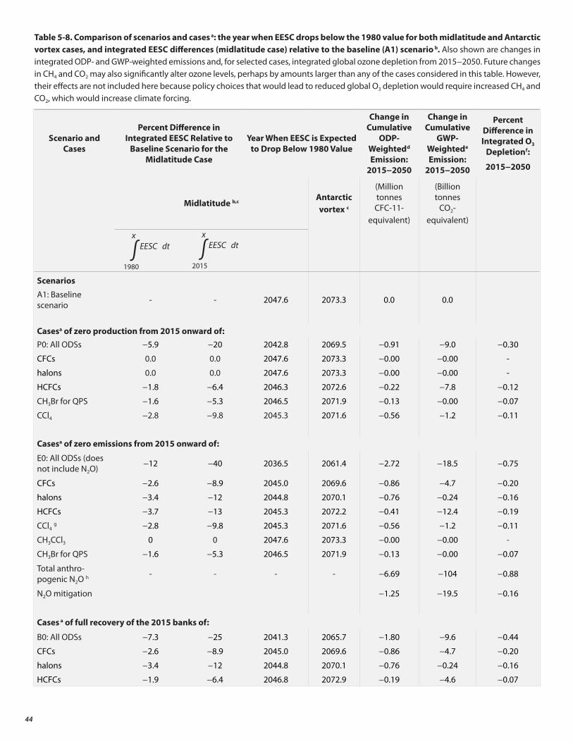
44
Table 5-8. Comparison of scenarios and cases a: the year when EESC drops below the 1980 value for both midlatitude and Antarctic vortex cases, and integrated EESC differences (midlatitude case) relative to the baseline (A1) scenario b. Also shown are changes in integrated ODP- and GWP-weighted emissions and, for selected cases, integrated global ozone depletion from 2015−2050. Future changes in CH4 and CO2 may also significantly alter ozone levels, perhaps by amounts larger than any of the cases considered in this table. However, their effects are not included here because policy choices that would lead to reduced global O3 depletion would require increased CH4 and CO2, which would increase climate forcing.
Scenario and Cases
Percent Difference in Integrated EESC Relative to
Baseline Scenario for the Midlatitude Case
Year When EESC is Expected to Drop Below 1980 Value
Change in Cumulative
ODP-Weightedd Emission:
2015−2050
Change in Cumulative
GWP-Weightede Emission:
2015−2050
Percent Difference in Integrated O3
Depletionf:
2015−2050
Midlatitude b,c Antarctic vortex c
(Million tonnes CFC-11-
equivalent)
(Billion tonnes
CO2-equivalent)
x
∫ EESC dt
1980
x
∫ EESC dt
2015
Scenarios
A1: Baseline scenario - - 2047.6 2073.3 0.0 0.0
Casesa of zero production from 2015 onward of: P0: All ODSs −5.9 −20 2042.8 2069.5 −0.91 −9.0 −0.30
CFCs 0.0 0.0 2047.6 2073.3 −0.00 −0.00 -
halons 0.0 0.0 2047.6 2073.3 −0.00 −0.00 -
HCFCs −1.8 −6.4 2046.3 2072.6 −0.22 −7.8 −0.12
CH3Br for QPS −1.6 −5.3 2046.5 2071.9 −0.13 −0.00 −0.07
CCl4 −2.8 −9.8 2045.3 2071.6 −0.56 −1.2 −0.11
Casesa of zero emissions from 2015 onward of:
E0: All ODSs (does not include N2O) −12 −40 2036.5 2061.4 −2.72 −18.5 −0.75
CFCs −2.6 −8.9 2045.0 2069.6 −0.86 −4.7 −0.20
halons −3.4 −12 2044.8 2070.1 −0.76 −0.24 −0.16
HCFCs −3.7 −13 2045.3 2072.2 −0.41 −12.4 −0.19
CCl4 g −2.8 −9.8 2045.3 2071.6 −0.56 −1.2 −0.11
CH3CCl3 0 0 2047.6 2073.3 −0.00 −0.00 -
CH3Br for QPS −1.6 −5.3 2046.5 2071.9 −0.13 −0.00 −0.07
Total anthro-pogenic N2O h - - - - −6.69 −104 −0.88
N2O mitigation −1.25 −19.5 −0.16
Cases a of full recovery of the 2015 banks of:
B0: All ODSs −7.3 −25 2041.3 2065.7 −1.80 −9.6 −0.44
CFCs −2.6 −8.9 2045.0 2069.6 −0.86 −4.7 −0.20
halons −3.4 −12 2044.8 2070.1 −0.76 −0.24 −0.16
HCFCs −1.9 −6.4 2046.8 2072.9 −0.19 −4.6 −0.07
45
Cases a of full recovery of the 2020 banks of:
B0: All ODSs −4.7 −16 2042.4 2066.8 −1.39 −8.1 −0.38
CFCs −1.5 −5.3 2045.6 2070.3 −0.64 −3.3 -
halons −2.0 −6.8 2045.4 2070.6 −0.56 −0.18 -
HCFCs −1.6 −5.5 2046.5 2072.7 −0.19 −4.6 -
CH3Br sensitivity:
Same as A1, but critical-use exemptions continue at 2012 levels
+0.2 +0.7 2047.8 2073.5 +0.02 +0.00 -
a Significance of ozone-depleting substances for future EESC was calculated in the hypothetical “cases” by setting production or emission to zero in 2015 and subsequent years or the bank of the ODS to zero in the year 2015 or 2020.
b EESC is integrated until it returns to 1980 levels, denoted as year “x.”c For midlatitude conditions, an average age-of-air of 3 years, corresponding fractional release values, and a bromine efficiency
factor (alpha) of 60 are assumed. For Antarctic vortex conditions, an average age-of-air of 5.5 years, corresponding fractional release values, and an alpha value of 65 are assumed. In all cases, age spectra are applied as in Newman et al. (2007).
d Semi-empirical ODPs from Table 5-2.e GWPs with 100-year time horizon (see Chapter 5, Appendix Table 5A-1).f Integrated globally averaged total column ozone changes are taken from 2-D model runs described in Chapter 5.g Banks are assumed to be zero. Emissions include uncertain sources such as possible fugitive emissions and unintended other emissions.h The integrated ODP- and GWP-weighted emissions correspond to the reduction of anthropogenic N2O emissions from a
business-as-usual case to a strong mitigation case (see text).
It is important to recognize that any future increases in CO2 and CH4 not only will have a substantial impact on climate forcing, but also are expected to lead to higher levels of globally averaged total ozone than if these greenhouse gases remained constant. So while CO2 and CH4 are likely not considered candidates for altering future ozone depletion themselves, it is important to be aware that policy options for halocarbon ODS and for N2O will be made against a backdrop of potentially large ozone changes due to CO2 and CH4. The effects on ozone due to increasing CO2 and CH4 are discussed in detail in Chapter 2; a summary of the important mechanisms and ozone responses is provided here.
For most of the scenarios examined, increases in ozone arising from CO2 and CH4 increases may be comparable to or larger than the additional depletion caused by N2O increases. This behavior can be seen from the 2-D model calculations of global total ozone using the RCP6.0 scenario shown in Figure 5-4 (bottom). This illustrates the individual effects of future increases in CO2 (red line), CH4 (yellow line), and N2O (green line) in the presence of decreasing ODS, and can be compared with the impact due to only the decreasing ODS (in which the GHGs are all fixed at 2000 levels, blue line). As shown by comparing the red, yellow, and green lines with the blue line in Figure 5-4, increasing CO2 leads to a substantial global ozone increase by 2100 (+2% relative to 1950) primarily due to stratospheric cooling, which reduces the ozone chemical loss rates (Haigh and Pyle, 1979). Note that these results are for global ozone and that more localized changes may differ (see below and Chapter 2). Another factor is that future CO2-induced stratospheric changes will indirectly affect ozone by somewhat mitigating the ozone depletion caused by N2O (see Figure ADM 6-1 and Section 2.4.3.1 of Chapter 2).
Compared to CO2, methane loading leads to a smaller global total ozone increase (yellow line in Figure 5-4, bottom). CH4 causes ozone to increase by: 1) mitigation of the chlorine-ozone loss cycles in the stratosphere, and 2) enhanced NOx-induced ozone production in the troposphere and lowermost stratosphere following CH4 oxidation (Brasseur and Solomon, 2005, and see Section 2.4.3.1 of Chapter 2). For total column ozone, these processes dominate the ozone reductions caused by the CH4-enhanced HOx-ozone loss cycles that are important primarily in the upper stratosphere (Revell et al., 2012). The slight decline of the CH4-induced total ozone change during the late 21st century in Figure 5-4 is caused by the decrease in methane in the RCP6.0 scenario. As atmospheric chlorine levels decline through the 21st century, future methane-induced changes in total ozone will be increasingly determined by the NOx-ozone production cycle in the troposphere and lowermost stratosphere. The large range in CH4 among the RCP scenarios, mainly due to the very high methane of RCP8.5 (Section 2.4.3.2 of Chapter 2), is projected to produce a large range of future tropospheric ozone responses. For example, in 2100, CH4 increases of 1.9–2.0 ppm (approximately the increase from present day to 2100 in RCP8.5) are projected to increase tropospheric column ozone by 3.5–5 DU (10–13%) (Brasseur et al., 2006; Kawase et al., 2011).
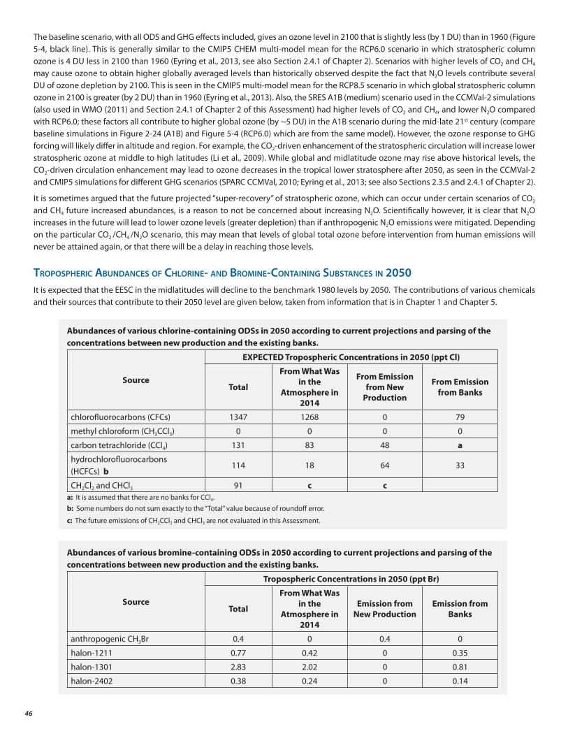
46
The baseline scenario, with all ODS and GHG effects included, gives an ozone level in 2100 that is slightly less (by 1 DU) than in 1960 (Figure 5-4, black line). This is generally similar to the CMIP5 CHEM multi-model mean for the RCP6.0 scenario in which stratospheric column ozone is 4 DU less in 2100 than 1960 (Eyring et al., 2013, see also Section 2.4.1 of Chapter 2). Scenarios with higher levels of CO2 and CH4 may cause ozone to obtain higher globally averaged levels than historically observed despite the fact that N2O levels contribute several DU of ozone depletion by 2100. This is seen in the CMIP5 multi-model mean for the RCP8.5 scenario in which global stratospheric column ozone in 2100 is greater (by 2 DU) than in 1960 (Eyring et al., 2013). Also, the SRES A1B (medium) scenario used in the CCMVal-2 simulations (also used in WMO (2011) and Section 2.4.1 of Chapter 2 of this Assessment) had higher levels of CO2 and CH4, and lower N2O compared with RCP6.0; these factors all contribute to higher global ozone (by ~5 DU) in the A1B scenario during the mid-late 21st century (compare baseline simulations in Figure 2-24 (A1B) and Figure 5-4 (RCP6.0) which are from the same model). However, the ozone response to GHG forcing will likely differ in altitude and region. For example, the CO2-driven enhancement of the stratospheric circulation will increase lower stratospheric ozone at middle to high latitudes (Li et al., 2009). While global and midlatitude ozone may rise above historical levels, the CO2-driven circulation enhancement may lead to ozone decreases in the tropical lower stratosphere after 2050, as seen in the CCMVal-2 and CMIP5 simulations for different GHG scenarios (SPARC CCMVal, 2010; Eyring et al., 2013; see also Sections 2.3.5 and 2.4.1 of Chapter 2).
It is sometimes argued that the future projected “super-recovery” of stratospheric ozone, which can occur under certain scenarios of CO2 and CH4 future increased abundances, is a reason to not be concerned about increasing N2O. Scientifically however, it is clear that N2O increases in the future will lead to lower ozone levels (greater depletion) than if anthropogenic N2O emissions were mitigated. Depending on the particular CO2 /CH4 /N2O scenario, this may mean that levels of global total ozone before intervention from human emissions will never be attained again, or that there will be a delay in reaching those levels.
tropospheric aBUndances of chlorine- and BroMine-containing sUBstances in 2050It is expected that the EESC in the midlatitudes will decline to the benchmark 1980 levels by 2050. The contributions of various chemicals and their sources that contribute to their 2050 level are given below, taken from information that is in Chapter 1 and Chapter 5.
Abundances of various chlorine-containing ODSs in 2050 according to current projections and parsing of the concentrations between new production and the existing banks.
Source
EXPECTED Tropospheric Concentrations in 2050 (ppt Cl)
Total
From What Was in the
Atmosphere in 2014
From Emission from New
Production
From Emission from Banks
chlorofluorocarbons (CFCs) 1347 1268 0 79
methyl chloroform (CH3CCl3) 0 0 0 0
carbon tetrachloride (CCl4) 131 83 48 a
hydrochlorofluorocarbons (HCFCs) b
114 18 64 33
CH2Cl2 and CHCl3 91 c ca: It is assumed that there are no banks for CCl4. b: Some numbers do not sum exactly to the “Total” value because of roundoff error.
c: The future emissions of CH2CCl2 and CHCl3 are not evaluated in this Assessment.
Abundances of various bromine-containing ODSs in 2050 according to current projections and parsing of the concentrations between new production and the existing banks.
Source
Tropospheric Concentrations in 2050 (ppt Br)
Total
From What Was in the
Atmosphere in 2014
Emission from New Production
Emission from Banks
anthropogenic CH3Br 0.4 0 0.4 0
halon-1211 0.77 0.42 0 0.35
halon-1301 2.83 2.02 0 0.81
halon-2402 0.38 0.24 0 0.14
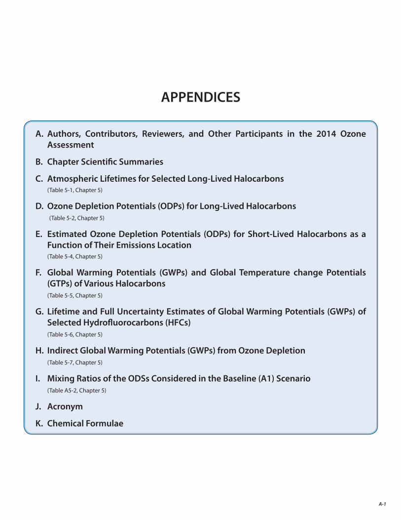
A-1
APPENDICES
A. Authors, Contributors, Reviewers, and Other Participants in the 2014 Ozone Assessment
B. Chapter Scientific Summaries
C. Atmospheric Lifetimes for Selected Long-Lived Halocarbons (Table 5-1, Chapter 5)
D. Ozone Depletion Potentials (ODPs) for Long-Lived Halocarbons (Table 5-2, Chapter 5)
E. Estimated Ozone Depletion Potentials (ODPs) for Short-Lived Halocarbons as a Function of Their Emissions Location (Table 5-4, Chapter 5)
F. Global Warming Potentials (GWPs) and Global Temperature change Potentials (GTPs) of Various Halocarbons
(Table 5-5, Chapter 5)
G. Lifetime and Full Uncertainty Estimates of Global Warming Potentials (GWPs) of Selected Hydrofluorocarbons (HFCs)
(Table 5-6, Chapter 5)
H. Indirect Global Warming Potentials (GWPs) from Ozone Depletion (Table 5-7, Chapter 5)
I. Mixing Ratios of the ODSs Considered in the Baseline (A1) Scenario (Table A5-2, Chapter 5)
J. Acronym
K. Chemical Formulae

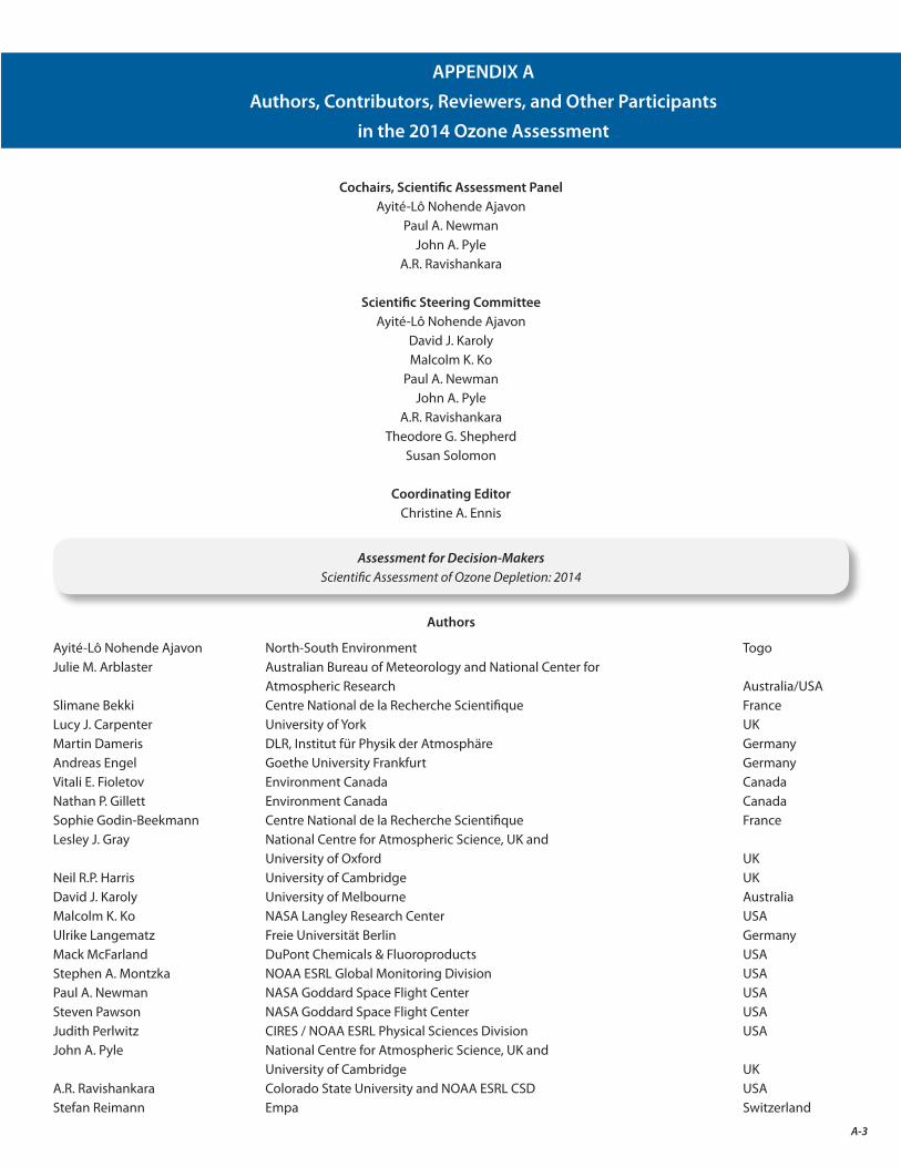
A-3
Cochairs, Scientific Assessment PanelAyité-Lô Nohende Ajavon
Paul A. NewmanJohn A. Pyle
A.R. Ravishankara
Scientific Steering CommitteeAyité-Lô Nohende Ajavon
David J. KarolyMalcolm K. Ko
Paul A. NewmanJohn A. Pyle
A.R. RavishankaraTheodore G. Shepherd
Susan Solomon
Coordinating EditorChristine A. Ennis
Assessment for Decision-MakersScientific Assessment of Ozone Depletion: 2014
Authors
Ayité-Lô Nohende Ajavon North-South Environment TogoJulie M. Arblaster Australian Bureau of Meteorology and National Center for Atmospheric Research Australia/USASlimane Bekki Centre National de la Recherche Scientifique FranceLucy J. Carpenter University of York UKMartin Dameris DLR, Institut für Physik der Atmosphäre GermanyAndreas Engel Goethe University Frankfurt GermanyVitali E. Fioletov Environment Canada CanadaNathan P. Gillett Environment Canada CanadaSophie Godin-Beekmann Centre National de la Recherche Scientifique FranceLesley J. Gray National Centre for Atmospheric Science, UK and University of Oxford UKNeil R.P. Harris University of Cambridge UKDavid J. Karoly University of Melbourne AustraliaMalcolm K. Ko NASA Langley Research Center USAUlrike Langematz Freie Universität Berlin GermanyMack McFarland DuPont Chemicals & Fluoroproducts USAStephen A. Montzka NOAA ESRL Global Monitoring Division USAPaul A. Newman NASA Goddard Space Flight Center USASteven Pawson NASA Goddard Space Flight Center USAJudith Perlwitz CIRES / NOAA ESRL Physical Sciences Division USAJohn A. Pyle National Centre for Atmospheric Science, UK and University of Cambridge UKA.R. Ravishankara Colorado State University and NOAA ESRL CSD USAStefan Reimann Empa Switzerland
APPENDIX A
Authors, Contributors, Reviewers, and Other Participants
in the 2014 Ozone Assessment
A-4
Theodore G. Shepherd University of Reading UKSusan Solomon Massachusetts Institute of Technology USAWolfgang Steinbrecht Deutscher Wetterdienst, Hohenpeissenberg GermanyDavid W.J. Thompson Colorado State University USAGuus J.M. Velders National Institute for Public Health and the Environment (RIVM) The NetherlandsDonald J. Wuebbles University of Illinois USA
Contributors
John S. Daniel NOAA ESRL Chemical Sciences Division USALucien Froidevaux Jet Propulsion Laboratory, California Institute of Technology USABradley D. Hall NOAA ESRL Global Monitoring Division USAMichaela I. Hegglin University of Reading UKNathaniel Livesey Jet Propulsion Laboratory, California Institute of Technology USARolf Müller Forschungszentrum Jülich GmbH GermanyRonald G. Prinn Massachusetts Institute of Technology USA Darryn W. Waugh The Johns Hopkins University USA
Reviewers
Stephen O. Andersen Institute for Governance & Sustainable Development USAPieter J. Aucamp EEAP Panel Liaison/Ptersa South AfricaGufran Beig Indian Institute of Tropical Meteorology IndiaGeir O. Braathen World Meteorological Organization SwitzerlandJohn P. Burrows University of Bremen GermanyPablo O. Canziani Pontificia Universidad Católica / CONICET ArgentinaMartyn P. Chipperfield University of Leeds UKJohn S. Daniel NOAA ESRL Chemical Sciences Division USAChristine A. Ennis NOAA ESRL Chemical Sciences Division USADavid W. Fahey NOAA ESRL Chemical Sciences Division USALucien Froidevaux Jet Propulsion Laboratory, California Institute of Technology USAAnnie Gabriel Department of the Environment AustraliaMarco González Sistemas de Energia Costa RicaMichaela I. Hegglin University of Reading UKKenneth W. Jucks NASA Headquarters USALambert J.M. Kuijpers TEAP Panel Liaison / Technical University Eindhoven The NetherlandsMichael J. Kurylo Universities Space Research Association / Goddard Earth Sciences, Technology, and Research USAMartin R. Manning New Zealand Climate Change Research Institute New ZealandAmanda C. Maycock University of Cambridge UKPauline M. Midgley University of Bern SwitzerlandOlaf Morgenstern National Institute of Water and Atmospheric Research New ZealandRolf Müller Forschungszentrum Jülich GmbH GermanyHiroaki Naoe Japan Meteorological Agency JapanThomas Peter Swiss Federal Institute of Technology (ETH) SwitzerlandDavid Plummer Environment Canada CanadaLorenzo M. Polvani Columbia University USARonald G. Prinn Massachusetts Institute of Technology USAJose M. Rodriguez NASA Goddard Space Flight Center USARoss J. Salawitch University of Maryland USAMegumi Seki UNEP Ozone Secretariat KenyaRajendra Shende TERRE Policy Centre IndiaWilliam T. Sturges University of East Anglia UKSaid Ali Thauobane Université des Comores ComorosTimothy J. Wallington Ford Motor Company USADarryn W. Waugh The Johns Hopkins University USARay F. Weiss University of California San Diego/Scripps Institution of Oceanography USA
A-5
Shigeo Yoden Kyoto University JapanDurwood Zaelke Institute for Governance & Sustainable Development USALingxi Zhou Chinese Meteorological Administration China
[Lead Authors in plain font; Chapter Editors in italics.]
Chapter 1: Update on Ozone-Depleting Substances (ODSs) and Other Gases of Interest to the Montreal ProtocolLucy J. Carpenter University of York UKStefan Reimann Empa SwitzerlandAndreas Engel Goethe University Frankfurt GermanyStephen A. Montzka NOAA ESRL Global Monitoring Division USA
Chapter 2: Update on Global Ozone: Past, Present, and FutureSteven Pawson NASA Goddard Space Flight Center USAWolfgang Steinbrecht Deutscher Wetterdienst, Hohenpeissenberg GermanyVitali E. Fioletov Environment Canada CanadaUlrike Langematz Freie Universität Berlin Germany
Chapter 3: Update on Polar Ozone: Past, Present, and FutureMartin Dameris DLR, Institut für Physik der Atmosphäre GermanySophie Godin-Beekmann Centre National de la Recherche Scientifique FranceJudith Perlwitz CIRES / NOAA ESRL Physical Sciences Division USASlimane Bekki Centre National de la Recherche Scientifique France
Chapter 4: Stratospheric Ozone Changes and ClimateJulie M. Arblaster Australian Bureau of Meteorology and National Center for Atmospheric Research Australia/USANathan P. Gillett Environment Canada CanadaLesley J. Gray Oxford University UKDavid W.J. Thompson Colorado State University USA
Chapter 5: Scenarios and Information for PolicymakersNeil R.P. Harris Cambridge University UKDonald J. Wuebbles University of Illinois USAMack McFarland DuPont Chemicals & Fluoroproducts USAGuus J.M. Velders RIVM (National Institute for Public Health and the Environment) The Netherlands
Twenty Questions and Answers About the Ozone Layer: 2014 UpdateMichaela I. Hegglin University of Reading UK
All Authors, Contributors, and ReviewersScientific Assessment of Ozone Depletion: 2014
Jon Abbatt CanadaAyité-Lô Nohende Ajavon TogoHideharu Akiyoshi JapanJoan M. Alexander USASimon Alexander AustraliaStephen O. Andersen USAValentina Aquila USAJulie M. Arblaster Australia/USA
Matthew Ashfold MalaysiaGhassem Asrar USAPieter J. Aucamp South AfricaAlkiviadis F. Bais GreeceMark P. Baldwin UKElizabeth A. Barnes USASteven L. Baughcum USAGufran Beig India
Lead Authors and Chapter EditorsScientific Assessment of Ozone Depletion: 2014
A-6
Slimane Bekki FrancePeter Bernath USATina Birmpili UNEPThomas Birner USADonald R. Blake USAGreg Bodeker New ZealandRumen D. Bojkov GermanyGeir O. Braathen WMOPeter Braesicke GermanyStefan Brönnimann SwitzerlandDominik Brunner SwitzerlandJames B. Burkholder USAJohn P. Burrows GermanyNeal Butchart UKAmy H. Butler USAWenju Cai AustraliaFrancesco Cairo ItalyNatalia Calvo SpainPablo O. Canziani ArgentinaLucy J. Carpenter UKKenneth S. Carslaw UKAndrew J. Charlton-Perez UKWissam Chehade GermanyMartyn P. Chipperfield UKBo Christiansen DenmarkIrene Cionni ItalyCathy Clerbaux FranceMelanie Coldewey-Egbers GermanyMartin Dameris GermanyJohn S. Daniel USAJos de Laat The NetherlandsAndy Delcloo BelgiumSandip Dhomse UKSusana B. Diaz ArgentinaMarcel Dorf GermanyAnne R. Douglass USAGeoffrey S. Dutton USARichard S. Eckman USANawo Eguchi JapanJames William Elkins USAAndreas Engel GermanyInes Engel GermanyChristine A. Ennis USAVeronika Eyring GermanyDavid W. Fahey USAVitali E. Fioletov CanadaEric L. Fleming USAPiers M. Forster UKPaul J. Fraser AustraliaStacey M. Frith USALucien Froidevaux USAJan Fuglestvedt NorwayMasatomo Fujiwara JapanJohn C. Fyfe CanadaAnnie Gabriel AustraliaLenah Gaoetswe BotswanaChaim I. Garfinkel IsraelHella Garny GermanyMarvin A. Geller USAEdwin P. Gerber USA
Andrew Gettelman USATomasz Gierczak PolandManuel Gil-Ojeda SpainNathan P. Gillett CanadaSophie Godin-Beekmann FranceMarco González Costa RicaLesley J. Gray UKKevin M. Grise USAJens-Uwe Grooß GermanySerge Guillas UKJoanna D. Haigh UKBradley D. Hall USASteven C. Hardiman UKNeil R.P. Harris UKBirgit Hassler USAAlain Hauchecorne FrancePeter Haynes UKMichaela I. Hegglin UKFrançois Hendrick BelgiumPeter Hitchcock UKØivind Hodnebrog NorwayLarry Horowitz USARyan Hossaini UKJianxin Hu ChinaNathalie Huret FranceDale F. Hurst USAIolanda Ialongo FinlandMohammad Ilyas MalaysiaFranz Immler BelgiumIvar S.A. Isaksen NorwayCharles H. Jackman USAMichal Janouch Czech RepublicAshley Jones Canada Julie M. Jones UKKenneth W. Jucks USADavid J. Karoly AustraliaAlexey Yu. Karpechko FinlandYasuko Kasai JapanPhilippe Keckhut FranceSergey Khaykin RussiaDoug Kinnison USAAndrew R. Klekociuk AustraliaJeff R. Knight UKMalcolm K. Ko USAYutaka Kondo JapanKarin Kreher New ZealandKirstin Krüger NorwayPaul B. Krummel AustraliaLambert J.M. Kuijpers The NetherlandsMarkus Kunze GermanyMichael J. Kurylo USAPaul J. Kushner CanadaErkki Kyrölä FinlandGabriela Lakkis ArgentinaShyam Lal IndiaJean-François Lamarque USATom Land USAUlrike Langematz GermanyJohannes C. Laube UKKatharine S. Law France
A-7
Franck Lefèvre FranceBernard Legras FranceJos Lelieveld GermanyQing Liang USAEun-Pa Lim AustraliaJintai Lin ChinaNathaniel Livesey USADiego Loyola GermanyEmmanuel Mahieu BelgiumDesmond Manatsa ZimbabweGloria L. Manney USAMartin R. Manning New ZealandElisa Manzini GermanyBella Maranion USADaniel R. Marsh USAAmanda C. Maycock UKMack McFarland USACharles McLandress CanadaChris McLinden CanadaJohan Mellqvist SwedenMichael P. Meredith UKPauline M. Midgley SwitzerlandDaniel M. Mitchell UKMario J. Molina USAStephen A. Montzka USAOlaf Morgenstern New ZealandJens Mühle USARolf Müller GermanyHiroaki Naoe JapanThando Ndarana South AfricaPaul A. Newman USAOle John Nielsen DenmarkSimon O’Doherty UKKeiichi Ohnishi JapanLuke D. Oman USAVladimir L. Orkin USAAndrew Orr UKYvan J. Orsolini NorwaySteven Pawson USAJuan Carlos Peláez CubaStuart A. Penkett UKJudith Perlwitz USAThomas Peter SwitzerlandIrina Petropavlovskikh USAKlaus Pfeilsticker GermanyDaniel Phoenix USADamaris K. Pinheiro BrazilGiovanni Pitari ItalyMichael C. Pitts USADavid Plummer CanadaLorenzo M. Polvani USAJean-Pierre Pommereau FranceLamont R. Poole USARobert W. Portmann USAMichael J. Prather USAMichael Previdi USARonald G. Prinn USAJohn A. Pyle UKBirgit Quack GermanyB. Rajakumar India
S. Ramachandran IndiaV. Ramaswamy USACora Randall USAWilliam Randel USAMarilyn Raphael USAA.R. Ravishankara USAStefan Reimann SwitzerlandJames Renwick New ZealandLaura Revell SwitzerlandMarkus Rex GermanyRobert C. Rhew USAHarald E. Rieder AustriaMartin Riese GermanyMatt Rigby UKVincenzo Rizi ItalyAlan Robock USAJose M. Rodriguez USAEugene Rozanov SwitzerlandVladimir Ryabinin SwitzerlandAlfonso Saiz-Lopez SpainTakatoshi Sakazaki JapanRoss J. Salawitch USAMichelle L. Santee USARobert Sausen GermanySue Schauffler USARobyn Schofield AustraliaDian J. Seidel USAMegumi Seki UNEPWilliam Seviour UKJonathan Shanklin UKTiffany A. Shaw USARajendra Shende IndiaTheodore G. Shepherd UKKiyotaka Shibata JapanKeith Shine UKMasato Shiotani JapanMichael Sigmond CanadaPeter Simmonds UKIsla R. Simpson USAIsobel J. Simpson USARajiv R. Singh USABjörn-Martin Sinnhuber GermanyKaren L. Smith USASusan Solomon USASeok-Woo Son KoreaJohannes Staehelin SwitzerlandWolfgang Steinbrecht GermanyGabriele P. Stiller GermanyRichard S. Stolarski USAWilliam T. Sturges UKTove M. Svendby NorwayNeil C. Swart CanadaDavid W. Tarasick CanadaSusann Tegtmeier GermanySaid Ali Thauobane ComorosLarry W. Thomason USADavid W.J. Thompson USASimone Tilmes USAOwen Brian Toon USAMatthew B. Tully Australia
A-8
Liaisons of Sponsoring OrganizationsGeir O. Braathen World Meteorological Organization Switzerland
Tina Birmpili United Nations Environment Programme KenyaA.R. Ravishankara National Oceanic and Atmospheric Administration USA
Kenneth W. Jucks National Aeronautics and Space Administration USAClaus Brüning European Commission Belgium
Assessment Coordinator and Technical EditorChristine A. Ennis CIRES/NOAA ESRL Chemical Sciences Division USA
Publication/Graphics Design and LayoutDebra A. Dailey-Fisher NOAA ESRL Chemical Sciences Division USA
Conference Coordination and DocumentationChristine A. Ennis CIRES/NOAA ESRL Chemical Sciences Division USA
Geir O. Braathen World Meteorological Organization SwitzerlandDebra A. Dailey-Fisher NOAA ESRL Chemical Sciences Division USA
John A. Pyle University of Cambridge UK
Conference SupportDebra Dailey-Fisher NOAA ESRL Chemical Sciences Division USA
Jennifer Fox NOAA ESRL Chemical Sciences Division USA Jeanne S. Waters NOAA ESRL Chemical Sciences Division USA
Kathy A. Thompson CSC USAChantal Renaudot World Meteorological Organization Switzerland
Alice Wood University of Cambridge UKMegumi Seki UNEP Ozone Secretariat Kenya
James S. Curlin UNEP Division of Technology, Industry, and Economics FranceBenedictine Desbois UNEP Division of Technology, Industry, and Economics France
Computing and Networking SupportRichard J. Tisinai CIRES/NOAA ESRL Chemical Sciences Division USA
Jennifer Fox NOAA ESRL Chemical Sciences Division USA
Document DistributionJeanne S. Waters NOAA ESRL Chemical Sciences Division USA
Debra A. Dailey-Fisher NOAA ESRL Chemical Sciences Division USASuzette M. Milano-Schoser NOAA ESRL Chemical Sciences Division USA
Megumi Seki UNEP Ozone Secretariat KenyaKathleen Creavalle UNEP Ozone Secretariat Kenya
Geir O. Braathen/Chantal Renaudot World Meteorological Organization Switzerland
Reference Research and EditingScout D. Ennis CIRES/NOAA ESRL Chemical Sciences Division USAZita N. Toth STC and NOAA ESRL Chemical Sciences Division USA
John Turner UKJoachim Urban SwedenRonald van der A The NetherlandsGuus J.M. Velders The NetherlandsDaniel P. Verdonik USAJean-Paul Vernier USAMartin K. Vollmer SwitzerlandPeter von der Gathen GermanyChristian von Savigny GermanyTimothy J. Wallington USADarryn W. Waugh USAAnn R. Webb UKMark Weber GermanyDebra K. Weisenstein USARay F. Weiss USA
Laura J. Wilcox UKJeannette Wild USAElian Augusto Wolfram ArgentinaYutian Wu USADonald J. Wuebbles USAShi-Keng Yang USAShigeo Yoden JapanYoko Yokouchi JapanPaul J. Young UKShari A. Yvon-Lewis USADurwood Zaelke USAChristos S. Zerefos GreeceLingxi Zhou ChinaJerry Ziemke USA
A-9
Changes in the global atmospheric abundance of a substance are determined by the balance between its emissions and removal. Declines observed for ozone-depleting substances (ODSs) controlled under the Montreal Protocol are due to global emission reductions that have made emissions smaller than removals. Most ODSs are potent greenhouse gases. As the majority of ODSs have been phased out, demand for hydrochlorofluorocarbon (HCFC) and hydrofluorocarbon (HFC) substitutes for the substances controlled under the Montreal Protocol has increased; these are also greenhouse gases. HCFCs deplete much less ozone per kilogram emitted than chlorofluorocarbons (CFCs), while HFCs essentially deplete no ozone.
The amended and adjusted Montreal Protocol has continued to reduce emissions and atmospheric abundances of most controlled ozone-depleting substances. By 2012, the total combined abundance of anthropogenic ODSs in the troposphere (measured as Equivalent Chlorine) had decreased by nearly 10% from its peak value in 1994.
The contributions to the overall decline in tropospheric chlorine (Cl) and bromine (Br) from substances and groups of substances controlled and not controlled under the Montreal Protocol have changed since the previous Assessment. The observed declines in total tropospheric Cl and Br from controlled substances during the 5-year period 2008–2012 were 13.4 ± 0.9 parts per trillion (ppt)/yr and 0.14 ± 0.02 ppt/yr, respectively.11
Substances controlled under the Montreal Protocol• −13.5 ± 0.5 ppt Cl/yr from chlorofluorocarbons (CFCs) • −4.1 ± 0.2 ppt Cl/yr from methyl chloroform (CH3CCl3)• −4.9 ± 0.7 ppt Cl/yr from carbon tetrachloride (CCl4)• −0.07 ± 0.01 ppt Cl/yr from halon-1211• +9.2 ± 0.3 ppt Cl/yr from hydrochlorofluorocarbons (HCFCs)• −0.06 ± 0.02 ppt Br/yr from halons• −0.08 ± 0.02 ppt Br/yr from methyl bromide (CH3Br)
Substances not controlled under the Montreal Protocol• −1.7 ± 1.3 ppt Cl/yr from methyl chloride (CH3Cl)• +1.3 ± 0.2 ppt Cl/yr from very short-lived chlorine compounds (predominantly dichloromethane, CH2Cl2)
Tropospheric Chlorine
Total tropospheric chlorine from ODSs continued to decrease between 2009 and 2012 to 3300 parts per trillion (ppt) in 2012. The observed decline in controlled substances of 13.4 ± 0.9 ppt Cl/yr during 2008–2012 was in line with the A1 (baseline) scenario of the 2010 Assessment.
Of total tropospheric Cl in 2012:• CFCs, consisting primarily of CFC-11, -12, and -113, accounted for 2024 ± 5 ppt (about 61%) and are declining. Their relative
contribution is essentially unchanged from the 2010 Assessment (62% in 2008).
• CCl4 accounted for 339 ± 5 ppt (about 10%). While our current understanding of the budget of CCl4 is incomplete, mole fractions of CCl4 declined largely as projected based on prior observations and the A1 scenario of the 2010 Assessment during 2009–2012.
• HCFCs accounted for 286 ± 4 ppt (8.7%). In total, the rate of increase for the sum of HCFCs has slowed by 25% since 2008 and has been lower than projected in the 2010 Assessment.
• CH3CCl3, the largest contributor to the decrease in total tropospheric chlorine until around 2005, accounted for only 16 ± 1 ppt (0.5%). This is 50% less than in 2008 (32 ppt) and a 95% reduction from its mean contribution to the total Cl decline during the 1980s. The fraction is declining in line with the A1 scenario of the 2010 Assessment.
Chapter 1 Update on Ozone-Depleting Substances (ODSs) and Other Gases of Interest to the Montreal Protocol
scientific sUMMary
11 All uncertainties are one standard deviation unless otherwise specified.
APPENDIX B
Chapter Scientific Summaries
A-10
• CH3Cl accounted for 540 ± 5 ppt (about 16%) and has remained essentially constant since 2008. This gas is emitted predominantly from natural sources.
• Very short-lived compounds (VSLS) contribute approximately 3%.
Global emissions of HCFCs remain substantial, but relative emissions of individual constituents have changed notably since the last Assessment. Emissions of HCFC-22 have stabilized since 2008 at around 370 gigagrams per year (Gg/yr). HCFC-142b emissions decreased in the same period. In contrast emissions of HCFC-141b have increased since the last Assessment, in parallel with reported production and consumption in Article 5 Parties.
Estimated sources and sinks of CCl4 remain inconsistent with observations of its abundance. The estimate of the total global lifetime (26 years) combined with the observed CCl4 trend in the atmosphere (−1.1 to −1.4 ppt/yr in 2011–2012) implies emissions of 57 (40–74) Gg/yr, which cannot be reconciled with estimated emissions from net reported production. New evidence indicates that other poorly quantified sources, unrelated to reported production, could contribute to the currently unaccounted emissions.
Three CFCs (CFC-112, -112a, -113a) and one HCFC (HCFC-133a) have recently been detected in the atmosphere. These four chlorine-containing compounds are listed in the Montreal Protocol and contribute about 4 ppt or ~ 0.1% toward current levels of total chlorine, currently adding less than 0.5 ppt Cl/yr. Abundances of CFC-112 and CFC-112a are declining and those of CFC-113a and HCFC-133a are increasing. The sources of these chemicals are not known.
Stratospheric Inorganic Chlorine and Fluorine
Hydrogen chloride (HCl) is the major reservoir of inorganic chlorine (Cly) in the mid- to upper stratosphere. Satellite-derived measurements of HCl (50°N–50°S) in the mid- to upper stratosphere show a mean decline of 0.6% ± 0.1%/yr between 1997 and 2012. This is consistent with the measured changes in controlled chlorinated source gases. Variability in this decline is observed over shorter time periods based on column measurements above some ground-based sites, likely due to dynamic variability.
Measured abundances of stratospheric fluorine product gases (HF, COF2 , COClF) increased by about 1%/yr between 2008 and 2012. This is consistent with increases in measured abundances of fluorinated compounds and their degradation products. The increase was smaller than in the beginning of the 1990s, when the concentrations of fluorine-containing ODSs were increasing more rapidly.
Tropospheric Bromine
Total organic bromine from controlled ODSs continued to decrease in the troposphere and by 2012 was 15.2 ± 0.2 ppt, approximately 2 ppt below peak levels observed in 1998. This decrease was close to that expected in the A1 scenario of the 2010 Assessment and was primarily driven by declines in methyl bromide (CH3Br), with some recent contribution from an overall decrease in halons. Total bromine from halons had stopped increasing at the time of the last Assessment, and a decrease is now observable.
CH3Br mole fractions continued to decline during 2008–2012, and by 2012 had decreased to 7.0 ± 0.1 ppt, a reduction of 2.2 ppt from peak levels measured during 1996–1998. These atmospheric declines are driven primarily by continued decreases in total reported consumption of CH3Br from fumigation. As of 2009, reported consumption for quarantine and pre-shipment (QPS) uses, which are exempted uses (not controlled) under the Montreal Protocol, surpassed consumption for controlled (non-QPS) uses. As a result of the decrease in atmospheric CH3Br, the natural oceanic source is now comparable to the oceanic sink.
Stratospheric Inorganic Bromine
Total inorganic stratospheric bromine (Bry), derived from observations of bromine monoxide (BrO), was 20 (16–23) ppt in 2011, and had decreased at ~0.6 ± 0.1%/yr between peak levels observed in 2000–2001 and 2012. This decline is consistent with the decrease in total tropospheric organic Br based on measurements of CH3Br and the halons.
Equivalent Effective Stratospheric Chlorine (EESC)
EESC is a sum of chlorine and bromine derived from ODS tropospheric abundances weighted to reflect their expected depletion of stratospheric ozone. The growth and decline in EESC depends on a given tropospheric abundance propagating to the stratosphere with varying time lags (on the order of years) associated with transport. Therefore the EESC abundance, its peak timing, and its rate of decline, are different in different regions of the stratosphere.
By 2012, EESC had declined by about 10% in polar regions and about 15% in midlatitudes from their peak values, with CH3CCl3, CH3Br, and CFCs contributing approximately equally to these declines. This drop is about 40% of the decrease required for EESC in midlatitudes to return to the 1980 benchmark level, and about 20% of the decrease required for EESC in polar regions to return to the 1980 benchmark level.
A-11
Very Short-Lived Halogenated Substances (VSLS)
VSLS are defined as trace gases whose local lifetimes are comparable to, or shorter than, interhemispheric transport timescales and that have non-uniform tropospheric abundances. These local lifetimes typically vary substantially over time and space. As in prior Assessments, we consider species with annual mean lifetimes less than approximately 6 months to be VSLS. Of the VSLS identified in the current atmosphere, brominated and iodinated species are predominantly of oceanic origin, while the chlorinated species have significant industrial sources. These compounds will release their halogen atoms nearly immediately once they enter the stratosphere. The current contribution of chlorinated VSLS to Equivalent Chlorine (ECl) is about one-third as large as the contribution of VSLS brominated gases. Iodine from VSLS likely makes a minor contribution to ECl.
Total chlorinated VSLS source gases increased from 84 (70–117) ppt in 2008 to 91 (76–125) ppt in 2012 in the lower troposphere. Dichloromethane (CH2Cl2), a VSLS that has predominantly anthropogenic sources, accounted for the majority of this change, with an increase of ~60% over the last decade.
The estimated contribution of chlorinated VSLS to total stratospheric chlorine remains small. A lack of data on their concentrations in the tropical tropopause layer (TTL) limits our ability to quantify their contribution to the inorganic chlorine loading in the lower stratosphere. Current tropospheric concentrations of chlorinated VSLS imply a source gas injection of 72 (50–95) ppt, with 64 ppt from anthropogenic emissions (e.g., CH2Cl2, CHCl3, 1,2 dichloroethane (CH2ClCH2Cl), tetrachloroethene (CCl2CCl2)). The product gases are estimated to contribute 0–50 ppt giving a total of ~95 ppt (50–145 ppt) against a total of 3300 ppt of chlorine from long-lived ODSs entering the stratosphere.
There is further evidence that VSLS contribute ~5 (2–8) ppt to a total of ~20 ppt of stratospheric bromine. Estimates of this contribution from two independent approaches are in agreement. New data suggest that previous estimates of stratospheric Bry derived from BrO observations may in some cases have been overestimated, and imply a contribution of ~5 (2–8) ppt of bromine from VSLS. The second approach sums the quantities of observed, very short-lived source gases around the tropical tropopause with improved modeled estimates of VSLS product gas injection into the stratosphere, also giving a total contribution of VSLS to stratospheric bromine of ~5 (2–8) ppt.
Updated Lifetime Estimates
The uncertainties of estimated lifetimes for key long-lived ozone-depleting and related substances are better quantified following the SPARC Lifetimes Assessment (Stratosphere-troposphere Processes And their Role in Climate, 2013). Of note is the change in the estimated lifetime of CFC-11 (revised from 45 yr to 52 yr). The estimate of the total global lifetime of CCl4 (26 yr) remains unchanged from the previous Assessment, although estimates of the relative importance of the multiple loss processes have been revised.
Other Trace Gases That Directly Affect Ozone and Climate
The emissions of CFCs, HCFCs, and HFCs in terms of their influence on climate (as measured by gigatonnes of carbon dioxide (CO2)-equivalent emissions) were roughly equal in 2012. However, the emissions of HFCs are increasing rapidly, while the emissions of CFCs are going down and those of HCFCs are essentially unchanged. The 100-year GWP-weighted emissions for the sum of CFC, HCFC, and HFC emissions was 2.2 Gt CO2-equivalent in 2012. The sum of GWP-weighted emissions of CFCs was 0.73 ± 0.25 Gt CO2-equivalent/yr in 2012 and has decreased on average by 11.0 ± 1.2%/yr from 2008 to 2012. The sum of HCFC emissions was 0.76 ± 0.12 Gt CO2-equivalent/yr in 2012 and has been essentially unchanged between 2008 and 2012. Finally, the sum of HFC emissions was 0.69 ± 0.12 Gt CO2-equivalent/yr in 2012 and has increased on average by 6.8 ± 0.9%/yr from 2008 to 2012. The HFC increase partially offsets the decrease by CFCs. Current emissions of HFCs are, however, are less than 10% of peak CFC emissions in the early 1990s (>8 Gt CO2-equivalent/yr).
From 2008 to 2012 the global mean mole fraction of nitrous oxide (N2O), which leads to ozone depletion in the stratosphere, increased by 3.4 parts per billion (ppb), to 325 ppb. With the atmospheric burden of CFC-12 decreasing, N2O is currently the third most important long-lived greenhouse gas contributing to radiative forcing (after CO2 and methane (CH4 )).
Methane (CH4) is an important greenhouse gas and influences stratospheric ozone. In 2012 the average background global mole fraction of CH4 was 1808 ppb, with a growth rate of 5–6 ppb/yr from 2008 to 2012. This is comparable to the 2006–2008 period when the CH4 growth rate began increasing again after several years of near-zero growth. The renewed increase is thought to result from a combination of increased CH4 emissions from tropical and high-latitude wetlands together with increasing anthropogenic (fossil fuel) emissions, though the relative contribution of the wetlands and fossil fuel sources is uncertain.
Hydrofluorocarbons (HFCs) used as ODS substitutes are increasing in the global atmosphere. The most abundant HFC, HFC-134a, reached a mole fraction of nearly 68 ppt in 2012 with an increase of 5 ppt/yr (7.6%) in 2011–2012. HFC-125, -143a, and -32 have similar or even higher relative growth rates than HFC-134a, but their current abundances are considerably lower.
Worldwide emissions of HFC-23, a potent greenhouse gas and by-product of HCFC-22 production, reached a maximum of ~15 Gg in 2006, decreased to ~9 Gg in 2009, and then increased again to reach ~13 Gg/yr in 2012. While efforts in non-Article 5 Parties mitigated an increasing portion of HFC-23 emissions through 2004, the temporary decrease in emissions after 2006 is consistent with
A-12
destruction of HFC-23 in Article 5 Parties owing to the Clean Development Mechanism (CDM) of the Kyoto Protocol. The average global mole fraction of HFC-23 reached 25 ppt in 2012, with an increase of nearly 1 ppt/yr in recent years.
Mole fractions of sulfur hexafluoride (SF6), nitrogen trifluoride (NF3), and sulfuryl fluoride (SO2F2) increased in recent years. Global averaged mole fractions of SF6 reached 7.6 ppt in 2012, with an annual increase of 0.3 ppt/yr (4%/yr). Global averaged mole fractions of NF3 reached 0.86 ppt in 2011, with an annual increase of 0.1 ppt/yr (12%/yr). Global averaged mole fractions of SO2F2 reached 1.8 ppt in 2012, with an annual increase of 0.1 ppt/yr (5%/yr). The considerable increases for these entirely anthropogenic, long-lived substances are caused by ongoing emissions.
Past Changes in Total Column Ozone
This chapter deals with the evolution of global ozone outside of the polar regions. The increase of ozone-depleting substance (ODS) concentrations caused the large ozone decline observed from 1980 to the mid-1990s. Since the late 1990s, concentrations of ODSs have been declining due to the successful implementation of the Montreal Protocol. As reported in the last Assessment, global ozone levels have remained stable since 2000. Ozone columns observed in the last four years have largely remained in the range observed since 2000.
Over the next decades we expect increasing global-mean stratospheric ozone columns, as ODSs decline further. Climate change and emissions of greenhouse gases, especially carbon dioxide (CO2 ), methane (CH4 ), and nitrous oxide (N2O), also affect the evolution of global stratospheric ozone, particularly in the second half of the 21st century, when ODS concentrations are expected to be low.
• Compared to 1964–1980 total column ozone, ground-based and space-based observations show that present-day (circa 2008–2013) ozone columns are: • lower by about 2% for the near-global average (60°S–60°N), compared to 2.5% reported in the last Assessment; • lower by about 3.5% in the Northern Hemisphere (35°N–60°N), as reported in the last Assessment;• lower by about 6% in the Southern Hemisphere (35°S–60°S), as reported in the last Assessment. The larger depletion in the
Southern Hemisphere is linked to the Antarctic ozone hole; and • almost unchanged in the tropics (20°S–20°N), as in the last Assessment.
• Ground- and space-based observations indicate that near-global (60°S–60°N) column ozone has increased by around 1% ± 1.7% (2 sigma) between 2000 and 2013. However, there is substantial disagreement among the data sets about the magnitude and statistical significance of this increase. Two out of three independent data sets show increases at the upper end; one recently updated data set shows an increase at the lower end. The CCMVal-2 multi-model mean predicts a 1% increase between 2000 and 2013 for the near-global (60°S–60°N) column ozone.
• Total column ozone (dominated by lower stratospheric ozone) displays large, dynamically forced year-to-year variability in the middle and high latitudes, exemplified by unusually high ozone in 2010 and low ozone in 2011 in the Northern Hemisphere, and low ozone in 2006 in the Southern Hemisphere. The recent decline (15% since 1997) in concentrations of ODSs, as described by Equivalent Effective Stratospheric Chlorine (EESC), is expected to have had only a small impact on total ozone recovery (approximately 3 Dobson units (DU), or 1%, since 2000). Separation of the small recent ODS-related ozone increase from the large natural variability (up to 15 DU or 5% change from one year to the next) can currently not be made with a high level of confidence.
Past Changes in Ozone Profiles
Additional and improved data sets have strengthened our ability to assess ozone profile changes over the last 10 to 15 years. Data from the upper stratosphere now confirm the significance of ozone increases that were already suggested in the last Assessment. Large ozone variability in the lower stratosphere complicates the identification of long-term ozone changes in this region. Chemistry-climate model (CCM) simulations that include realistic time variations of greenhouse gas (GHG) and ODS concentrations capture changes in the ozone profile that agree quite well with those observed. These CCM simulations provide a means of attributing changes in ozone to different processes.
• Measurements show a statistically significant increase in upper stratospheric ozone (35–45 km altitude) in middle latitudes and the tropics since around 2000. Following a large observed decline of 5–8% per decade through the 1980s and middle 1990s, ozone has increased by 2.5–5% per decade over the 2000 to 2013 period.
• About half of the upper stratospheric ozone increase after 2000 can be attributed to the decline of ODS since the late 1990s. Increasing CO2 concentrations have led to a cooling of the upper stratosphere. CCM simulations reveal that, between the 1980s and the present this has contributed to an increase in ozone concentrations. Before the middle 1990s, this ozone increase was substantially
Chapter 2 Update on Global Ozone: Past, Present, and Future
scientific sUMMary
A-13
smaller than the ozone decrease caused by ODS increases. From 2000 to 2013, the ozone increase arising from the decline in ODS concentrations is of comparable magnitude to that caused by upper stratospheric cooling.
• As reported in the last Assessment (WMO, 2011), CCMs consistently show a long-term decline of ozone in the lowermost tropical stratosphere by up to 20% between 1960 and 2060. This modeled ozone decline is caused by an increase in the strength of upwelling in the tropical lower stratosphere. This increased upwelling is associated with a strengthening Brewer-Dobson circulation caused by GHG-induced climate change.
• In-situ and space-based observations reveal that ozone concentrations in the lowermost tropical stratosphere have declined by as much as 10% between 1984 and 2005. There are several additional data sets available since 2002. Continued ozone decreases are not detected in the presence of large natural variability during 2002–2013. This observed behavior is consistent with that computed in CCMs, which also show periods of strong interannual and decadal variability.
Future Ozone Changes
The chemistry-climate model simulations used in the last Assessment are still the main source for projection of future ozone levels and the dates of return of ozone to 1980 levels. Declining ODS concentrations, upper stratospheric cooling because of increased CO2, and the possible strengthening of the Brewer-Dobson circulation from climate change are all likely to affect recovery of global column ozone, with different relative contributions in various latitude regions.
• Estimates of the likely return dates of total column ozone concentrations to their 1980 values have not changed since the last Assessment. The best estimates are:• by midcentury for global mean annually averaged ozone;• between 2015 and 2030 for annually averaged Northern Hemisphere midlatitude ozone;• between 2030 and 2040 for annually averaged Southern Hemisphere midlatitude ozone; and• for annual average tropical column ozone, slowly increasing until the middle of the 21st century, before leveling off at values
about 0–3% below 1980s columns.
• The updated lifetimes estimated for ODSs in the SPARC lifetimes report have no significant impact on model projections of future ozone evolution.
• Projections of future ozone levels depend substantially on the assumed scenario of greenhouse gas (GHG) emissions, especially in the later half of the 21st century. Six chemistry-climate model simulations show that projected total ozone columns in 2100 differ by up to 20 DU or 7% in the global average, by up to 40 DU or 12% in midlatitudes, and by up to 10 DU or 4% in the tropics between minimum and maximum radiative forcing Representative Concentration Pathway scenarios for future CO2, N2O, and CH4 emissions. These new estimates of scenario uncertainty are broadly consistent with previous estimates from different models and scenarios reported in the last Assessment. Our confidence in the magnitude of this scenario uncertainty remains low because of the small number of models and scenarios assessed.
• Part of the scenario uncertainty in future column ozone is due to differences in emissions of N2O and CH4 between different scenarios. Increases of stratospheric N2O and CH4 impact the chemical cycles relevant for ozone. Higher N2O emissions tend to reduce column ozone, whereas higher CH4 tends to increase column ozone, each by a few percent from 2020 to 2100. The magnitude of these effects on ozone is comparable to what is expected from stratospheric cooling by CO2 increases. The influence of each individual trace gas on ozone also depends on emissions of the others, meaning that their impacts on ozone are strongly scenario dependent.
• Given that ODS levels remain high, a large enhancement of stratospheric sulfate aerosol in the next decade, e.g., due to a volcanic eruption of the same size as Mt. Pinatubo, could result in chemical losses of at least 2% in total ozone columns over much of the globe. Confidence in this conclusion is strengthened because the long-standing puzzle about the midlatitude hemispheric asymmetry in the midlatitude ozone response to Mt. Pinatubo aerosols is now much better understood. Studies have shown that enhanced ozone transport in the Brewer-Dobson circulation more than compensated the enhanced chemical loss in the Southern Hemisphere.
Polar Ozone Changes
As stated in the previous Assessments, ozone-depleting substance (ODS) levels reached a maximum in the polar regions around the beginning of this century and have been slowly decreasing since then, consistent with the expectations based on compliance
Chapter 3 Update on Polar Ozone: Past, Present, and Future
scientific sUMMary
A-14
with the Montreal Protocol and its Amendments and adjustments. Considering the current elevated levels of ODSs, and their slow rate of decrease, changes in the size and depth of the Antarctic ozone hole and in the magnitude of the Arctic ozone depletion since 2000 have been mainly controlled by variations in temperature and dynamical processes.
· Over the 2010–2013 period, the Antarctic ozone hole continued to appear each spring. The continued occurrence of an Antarctic ozone hole is expected because ODS levels have declined by only about 10% from the peak values reached at the beginning of this century.
· Larger year-to-year variability of Antarctic springtime total ozone was observed over the last decade compared to the 1990s. The main driver of this pronounced variability has been variations in meteorological processes, notably the occurrence of dynamically induced disturbances of the Antarctic polar vortex.
· A small increase of about 10–25 Dobson units (DU) in springtime Antarctic total ozone since 2000 can be derived by subtracting an estimate of the natural variability from the total ozone time series. However, uncertainties in this estimate and in the total ozone measurements preclude definitive attribution of this increase to the reduction of ODSs over this period.
· Exceptionally low ozone abundances in the Arctic were observed in spring of 2011. These low ozone levels were due to anomalously persistent low temperatures and a strong, isolated polar vortex in the lower stratosphere that led to a large extent of halogen-induced chemical ozone depletion, and also to atypically weak transport of ozone-rich air into the vortex from lower latitudes. State-of-the-art chemical transport models (CTMs), which use observed winds and temperatures in the stratosphere together with known chemical processes, successfully reproduce the observed ozone concentrations.
Understanding of Polar Ozone Processes
Since the last Assessment, new laboratory measurements have strengthened our knowledge of polar ozone loss processes. Simulations using updated and improved models have been tested using the wealth of currently available measurements from satellites, ground-based networks, and dedicated campaigns.
• CTMs are generally able to reproduce the observed polar chlorine activation by stratospheric particles and the rate of the resulting photochemical ozone loss. Since the last Assessment, better constraint of a key photochemical parameter based on recent laboratory measurements, i.e., the ClOOCl (ClO dimer) photolysis cross section, has increased confidence in our ability to quantitatively model polar ozone loss processes in CTMs.
• Chemistry-climate models (CCMs), which calculate their own temperature and wind fields, do not fully reproduce the range of polar ozone variability. Most CCMs have limitations in simulating the temperature variability in polar regions in winter and spring, as well as the temporal and spatial variation of the polar vortex.
Future Changes in Polar Ozone
Projections of future ozone levels in this Assessment are mainly based on the CCM simulations used in the last Assessment. Individual studies using results from climate models provide new insights into the effects of carbon dioxide (CO2), nitrous oxide (N2O), and methane (CH4) on future polar ozone levels by the end of this century.
• Arctic and Antarctic ozone abundances are predicted to increase as a result of the expected reduction of ODSs. A return to values of ozone in high latitudes similar to those of the 1980s is likely during this century, with polar ozone predicted by CCMs to recover about 20 years earlier in the Arctic (2025–2035) than in the Antarctic (2045–2060). Updated ODS lifetimes have no significant effect on these estimated return dates to 1980 values.
• During the next few decades, while stratospheric halogens remain elevated, large Arctic ozone loss events similar to that observed in spring 2011 would occur again under similar long-lasting cold stratospheric conditions. CCM simulations indicate that dynamic variability will lead to occasional cold Arctic winters in the stratosphere but show no indication for enhanced frequency of their occurrence.
• Climate change will be an especially important driver for polar ozone change in the second half of the 21st century. Increases in CO2 concentrations will lead to a cooling of the stratosphere and increases in all greenhouse gases are projected to strengthen the transport of ozone-rich air to higher latitudes. Under conditions of low halogen loading both of these changes are anticipated to increase polar ozone amounts. The changes are expected to have a larger impact on ozone in the Arctic than in the Antarctic due to a larger sensitivity of dynamical processes in the Northern Hemisphere to climate change. Polar ozone levels at the end of the century might be affected by changing concentrations of N2O and CH4 through their direct impact on atmospheric chemistry. The atmospheric concentrations of both of these gases are projected to increase in most future scenarios, but these projections are very uncertain.
• Substantial polar ozone depletion could result from enhancements of sulfuric aerosols in the stratosphere during the next few decades when stratospheric halogen levels remain high. Such enhancements could result from major volcanic eruptions
A-15
in the tropics or deliberate “geoengineering” efforts. The surface area and number density of aerosol in polar regions are important parameters for heterogeneous chemistry and chlorine activation. The impact of sulfur dioxide (SO2) injection of either natural or anthropogenic origin on polar ozone depends on the halogen loading. In the next several decades, enhanced amounts of sulfuric acid aerosols would increase polar ozone depletion.
Since the last Assessment, new research has better quantified the impact of stratospheric ozone changes on climate. Additional model and observational analyses are assessed which examine the influence of stratospheric ozone changes on stratospheric temperatures and circulation, Southern Hemisphere tropospheric circulation and composition, surface climate, oceans, and sea ice.
• Stratospheric ozone changes are the dominant driver of observed globally averaged long-term temperature changes in the lower stratosphere. Between 1979 and 1995 global mean lower stratospheric temperature decreased by about 1 K but has since remained approximately constant.
• Models broadly reproduce the evolution of global mean lower stratospheric temperature change. Stratospheric ozone changes are the dominant driver of these changes, with volcanic aerosol driving episodic warming, and greenhouse gas increases having only a minor contribution.
• Observed mid- and upper-stratospheric temperatures decreased from 1979 to 2005, but the magnitude of the cooling is uncertain. A newly reprocessed data set of satellite measurements exhibits substantially different cooling trends compared to the existing data set. Models indicate that increasing greenhouse gases, as well as ozone changes, both made comparable contributions to observed cooling in the mid and upper stratosphere.
• There was little overall change in global lower stratospheric water vapor concentration between 2000 and 2012, based on satellite measurements, which show a decrease between 2000 and 2004 followed by an increase to 2012.
• The observed cooling of the Antarctic lower stratosphere since 1979 during austral spring is consistent with the average simulated cooling in models forced with observed ozone depletion. There is a large range in the magnitude of the simulated cooling, with models that underestimate the ozone depletion also underestimating the temperature trends.
• Climate models consistently predict a long-term increase in the strength of the Brewer-Dobson circulation due to greenhouse gas increases, with important impacts on stratospheric and tropospheric composition.
• The predicted increase in the strength of the Brewer-Dobson circulation extends throughout the depth of the stratosphere.
• Observations of changes in temperature, ozone, and trace gases over the past three to five decades are suggestive of increased upwelling in the tropical lower stratosphere, consistent with a strengthening of the shallow branch of the Brewer-Dobson circulation predicted by models. There is large uncertainty in changes in the deep branch of the Brewer-Dobson circulation inferred from observations in the mid and upper stratosphere.
• Stratospheric ozone recovery and an acceleration of the Brewer-Dobson circulation in the future would both tend to increase the global tropospheric ozone burden. The projected net changes in tropospheric ozone and other compounds vary regionally and are scenario and model dependent.
• Stratospheric temperature changes due to Antarctic ozone depletion are very likely the dominant driver of the observed changes in Southern Hemisphere tropospheric circulation in summer over recent decades, with associated surface climate and ocean impacts.
• The contribution of Antarctic ozone depletion to the observed increase in the Southern Annular Mode index in austral summer is substantially larger in most models than the contribution from greenhouse gas increases over the past three to five decades. An increase in this index corresponds to a decrease in atmospheric pressure at high latitudes, an increase at midlatitudes, and a poleward shift of the midlatitude jet. The role of ozone depletion is largest in summer. Observations and models suggest smaller Southern Annular Mode trends in other seasons.
• Stratospheric ozone depletion has likely contributed to the observed expansion of the Southern Hemisphere Hadley Cell in austral summer.
Chapter 4 Stratospheric Ozone Changes and Climate
scientific sUMMary
A-16
• Climate models simulate a poleward shift of the Southern Hemisphere midlatitude maximum in precipitation and a moistening of the subtropics in response to stratospheric ozone depletion in austral summer. There is some evidence of a consistent pattern of trends in observations.
• Observational and modeling studies present a broadly consistent picture of the ocean’s response to surface wind stress changes, which have likely been substantially caused by stratospheric ozone changes, with intensification of the subtropical ocean gyres and the meridional overturning circulations, and a subsurface warming. The impact of these wind stress changes on oceanic carbon uptake remains uncertain. The role of ocean eddies, which modify the ocean circulation and temperature response to wind stress changes, is better understood than at the time of the last Ozone Assessment, but remains a source of uncertainty.
• The influence of stratospheric ozone depletion on Antarctic sea ice increases reported in the last Ozone Assessment is not supported by a number of new coupled modeling studies. These suggest that ozone depletion drives a decrease in Southern Hemisphere sea ice extent and thus did not lead to the small observed increase. However, there is low confidence in this model result because of large uncertainties in the simulation of Antarctic sea ice.
• No robust link between stratospheric ozone changes and Northern Hemisphere tropospheric climate has been found, consistent with the conclusions of the previous Ozone Assessment.
• There is further evidence that in austral summer over the next 50 years, Antarctic stratospheric ozone recovery and increases in greenhouse gases will have opposite effects on the Southern Hemisphere tropospheric circulation, with associated surface climate and ocean impacts.
• Ozone recovery is expected to drive a weakening and equatorward shift of the midlatitude jet, while increases in greenhouse gases are expected to drive a strengthening and poleward shift of the jet. Under a low greenhouse gas emissions scenario, ozone recovery is expected to dominate the effect of greenhouse gas increases on Southern Hemisphere tropospheric circulation in austral summer to give a weakening and equatorward shift of the midlatitude jet over the next 50 years, whereas in a high emissions scenario the jet is projected to continue to strengthen and shift poleward.
• An equatorward shift in the Southern Hemisphere Hadley Cell boundary and extratropical rainfall in summer is simulated in response to ozone recovery. These changes offset a scenario-dependent fraction of projected greenhouse-gas induced changes in these variables.
• Simulations from multiple models indicate that if the concentrations of ozone-depleting substances (ODSs) had continued to increase in the absence of the Montreal Protocol, the enhanced ozone depletion from uncontrolled ODSs would be expected to have led to substantial additional cooling in the Antarctic polar stratosphere, with associated changes in Southern Hemisphere circulation and rainfall patterns.
• New estimates of global mean ozone radiative forcing due to emissions of ozone-depleting substances, which account for stratospheric ozone change and its indirect effect on tropospheric ozone, indicate a stronger surface cooling effect than that due to stratospheric ozone changes alone.
• The overall global mean ozone radiative forcing from the effects of ODS emissions on both tropospheric and stratospheric ozone is assessed to be −0.15 (−0.3 to 0) watts per square meter (W m-2) in 2011. Approximately three quarters of this results from ozone changes in the stratosphere.
• Models indicate that ODS-induced stratospheric ozone depletion has acted to decrease tropospheric ozone. This ODS-driven decrease in tropospheric ozone contributes to the overall negative ozone radiative forcing, although the magnitude is uncertain.
• The radiative forcing due to observed decreases in stratospheric ozone concentration alone is estimated to be −0.05 W m-2 (−0.15 to 0.05) W m-2 in 2011. A rapid adjustment to radiative forcing may also arise from cloud changes, resulting from the circulation changes driven by ODS-induced ozone depletion. The radiative effect of this cloud adjustment may be of a larger magnitude than the non-adjusted forcing.
• Uncertainty in future lower stratospheric ozone trends in the tropics precludes a confident assessment of the sign of future stratospheric ozone radiative forcing. Current models give a range of stratospheric ozone radiative forcing of −0.05 to +0.25 W m-2 in 2100 under a high greenhouse gas emissions scenario, which is generally suggestive of a slight warming contribution relative to present.
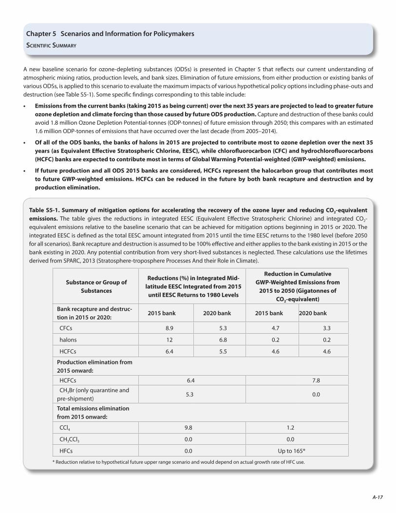
A-17
A new baseline scenario for ozone-depleting substances (ODSs) is presented in Chapter 5 that reflects our current understanding of atmospheric mixing ratios, production levels, and bank sizes. Elimination of future emissions, from either production or existing banks of various ODSs, is applied to this scenario to evaluate the maximum impacts of various hypothetical policy options including phase-outs and destruction (see Table S5-1). Some specific findings corresponding to this table include:
• Emissions from the current banks (taking 2015 as being current) over the next 35 years are projected to lead to greater future ozone depletion and climate forcing than those caused by future ODS production. Capture and destruction of these banks could avoid 1.8 million Ozone Depletion Potential-tonnes (ODP-tonnes) of future emission through 2050; this compares with an estimated 1.6 million ODP-tonnes of emissions that have occurred over the last decade (from 2005–2014).
• Of all of the ODS banks, the banks of halons in 2015 are projected to contribute most to ozone depletion over the next 35 years (as Equivalent Effective Stratospheric Chlorine, EESC), while chlorofluorocarbon (CFC) and hydrochlorofluorocarbons (HCFC) banks are expected to contribute most in terms of Global Warming Potential-weighted (GWP-weighted) emissions.
• If future production and all ODS 2015 banks are considered, HCFCs represent the halocarbon group that contributes most to future GWP-weighted emissions. HCFCs can be reduced in the future by both bank recapture and destruction and by production elimination.
Table S5-1. Summary of mitigation options for accelerating the recovery of the ozone layer and reducing CO2-equivalent emissions. The table gives the reductions in integrated EESC (Equivalent Effective Stratospheric Chlorine) and integrated CO2-equivalent emissions relative to the baseline scenario that can be achieved for mitigation options beginning in 2015 or 2020. The integrated EESC is defined as the total EESC amount integrated from 2015 until the time EESC returns to the 1980 level (before 2050 for all scenarios). Bank recapture and destruction is assumed to be 100% effective and either applies to the bank existing in 2015 or the bank existing in 2020. Any potential contribution from very short-lived substances is neglected. These calculations use the lifetimes derived from SPARC, 2013 (Stratosphere-troposphere Processes And their Role in Climate).
Substance or Group of Substances
Reductions (%) in Integrated Mid-latitude EESC Integrated from 2015
until EESC Returns to 1980 Levels
Reduction in Cumulative GWP-Weighted Emissions from
2015 to 2050 (Gigatonnes of CO2-equivalent)
Bank recapture and destruc-tion in 2015 or 2020:
2015 bank 2020 bank 2015 bank 2020 bank
CFCs 8.9 5.3 4.7 3.3
halons 12 6.8 0.2 0.2
HCFCs 6.4 5.5 4.6 4.6
Production elimination from 2015 onward:
HCFCs 6.4 7.8
CH3Br (only quarantine and pre-shipment)
5.3 0.0
Total emissions elimination from 2015 onward:
CCl4 9.8 1.2
CH3CCl3 0.0 0.0
HFCs 0.0 Up to 165*
* Reduction relative to hypothetical future upper range scenario and would depend on actual growth rate of HFC use.
Chapter 5 Scenarios and Information for Policymakers
scientific sUMMary
A-18
• The impact on ozone-layer recovery of further policy actions on already controlled ozone-depleting substances is becoming smaller. Nonetheless, if all ODS emissions – including those emanating from many widely dispersed banks – were to be stopped in 2015, then the return to 1980 midlatitude EESC values would be brought forward to 2036 compared with 2047 in the baseline scenario.
• Updated Ozone Depletion Potentials (ODPs) are almost all numerically smaller, ranging from no change (for carbon tetrachloride, CCl4) to more than a factor of two smaller (for CFC-115), with most of these smaller by 10–30% than the values reported in WMO (2011). These changes largely reflect the revised estimate for the atmospheric lifetime of CFC-11 (from 45 to 52 years) reported in SPARC (2013); CFC-11 is the reference gas in determining ODPs so this change affects all ODPs. Uncertainties in the atmospheric lifetimes, the fractional release values, and atmospheric chemistry generally result in overall uncertainties in ODPs on the order of 30% for the CFCs and CCl4, but are higher for HCFCs and halons (about 60% for the HCFCs and halon-1301, to over 80% for halon-1202 and halon-1211).
• New atmospheric model studies continue to emphasize that ODPs for very short-lived substances (VSLS) that contain bromine or chlorine are strongly dependent on the geographic location and season of emission. Impacts from VSLS are much larger (with ODPs approaching values of 1) if emissions occur in regions close to convective regions in the tropics. There is still insufficient research available to confidently compare the mitigation options of anthropogenic VSLS emissions with those of the longer-lived halogenated hydrocarbons; overall the VSLS have smaller ODPs than longer-lived ODS. However, if long-lived controlled halocarbons (and their banks) follow their projected decline, then chlorine- and bromine-containing anthropogenic VSLS emissions will play a relatively larger role in future ozone depletion, but the absolute effects are smaller than that of ODSs today while remaining uncertain.
• The projection of CCl4 remains more uncertain than projections for other ODSs due to our incomplete understanding of the current CCl4 budget (likely a missing source; see Chapter 1). In the scenarios examined (see table above), CCl4 human-related emissions from 2015 through 2050 are comparable to those of the HCFCs in terms of ODP-weighted emissions and are about 10% in terms of GWP-weighted emissions. It is expected that future emissions of CCl4 will remain an important factor in the evolution of EESC.
• The total anthropogenic emissions of methyl bromide (CH3Br) have declined in response to controls of the Montreal Protocol. Overall, reported consumption has gone down from ~70,000 tonnes/yr in the late 1990s to ~13,000 tonnes/yr in 2012.
• Quarantine and pre-shipment (QPS) uses of CH3Br are exempted uses (not controlled) by the Montreal Protocol and in 2012 constitute an annual consumption of CH3Br (~9,000 tonnes) that is larger than the annual consumption for 2012 from uses controlled by the Protocol (~4,000 tonnes). The elimination of future emissions from QPS uses could bring forward the date of EESC return to 1980 levels by 1.1 years, smaller than the 1.6 years estimated in the previous Assessment. Critical-use exemptions continue to be granted, but at levels significantly reduced compared with four years ago. A continuation of critical-use exemptions at the current level would delay the return of EESC to 1980 levels by 0.2 years.
• Carbon dioxide (CO2), nitrous oxide (N2O), and methane (CH4) are each important to climate forcing and to the levels of stratospheric ozone (see Chapter 2). In terms of the globally averaged ozone column, additional N2O leads to lower ozone levels, whereas additional CO2 and CH4 lead to higher ozone levels. Ozone depletion to date would have been greater if not for the historical increases in CO2 and CH4. The net impact on ozone recovery and future levels of stratospheric ozone thus depends on the future abundances of these gases. For many of the scenarios used in the most recent Intergovernmental Panel on Climate Change (IPCC) Assessment (IPCC, 2013), global ozone will increase to above pre-1980 levels due to future trends in the gases. Latitudinal and altitudinal responses are expected to vary. Note that scenarios used in IPCC consider a future with all three major greenhouse gases increasing and thus it is important to assess the net balance of these perturbations on stratospheric ozone.
• Global Warming Potentials (GWPs) for a range of halocarbons have been updated based on IPCC (2013) and SPARC (2013). The CO2 Absolute Global Warming Potential (AGWP; the denominator for the GWP of other greenhouse gases) has increased by 6% compared to the previous Assessment (WMO, 2011). As a result, GWP values for many non-CO2 greenhouse gases decreased slightly. GWPs also changed because of revised values for the lifetime and the radiative efficiency of the individual greenhouse gases. The revised SPARC-based lifetimes for a range of ODSs have been updated due to new analyses of observations and models and are included here; the largest differences in GWPs are found for CFC-11, CFC-115, halon-1301, halon-2402, and halon-1202. For hydrofluorocarbons (HFCs), some examples of the IPCC 100-year GWPs and the SPARC lifetime adjusted values are given below. The numbers in parentheses represent the effects of uncertainties in the SPARC lifetimes, radiative efficiency, and the AGWP for CO2 based on 90% confidence. In addition, the IPCC (2013) stated uncertainties in the 100-year GWP for HFC-134a is ±35% (90% confidence) as representative for similar gases. The IPCC and updated GWPs that use the SPARC lifetimes are consistent within their uncertainties.
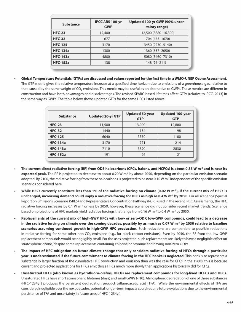
A-19
SubstanceIPCC AR5 100-yr
GWPUpdated 100-yr GWP (90% uncer-
tainty range)
HFC-23 12,400 12,500 (8880–16,300)
HFC-32 677 704 (453–1070)
HFC-125 3170 3450 (2230–5140)
HFC-134a 1300 1360 (857–2050)
HFC-143a 4800 5080 (3460–7310)
HFC-152a 138 148 (96–211)
• Global Temperature Potentials (GTPs) are discussed and values reported for the first time in a WMO-UNEP Ozone Assessment. The GTP metric gives the relative temperature increase at a specified time horizon due to emissions of a greenhouse gas, relative to that caused by the same weight of CO2 emissions. This metric may be useful as an alternative to GWPs. These metrics are different in construction and have both advantages and disadvantages. The revised SPARC-based lifetimes affect GTPs (relative to IPCC, 2013) in the same way as GWPs. The table below shows updated GTPs for the same HFCs listed above.
Substance Updated 20-yr GTPUpdated 50-year
GTP Updated 100-year
GTP
HFC-23 11,500 13,000 12,800
HFC-32 1440 154 98
HFC-125 6040 3350 1180
HFC-134a 3170 771 214
HFC-143a 7110 5390 2830
HFC-152a 191 26 21
• The current direct radiative forcing (RF) from ODS halocarbons (CFCs, halons, and HCFCs) is about 0.33 W m-2 and is near its expected peak. The RF is projected to decrease to about 0.20 W m-2 by about 2050, depending on the particular emission scenario adopted. By 2100, the radiative forcing from these halocarbons is projected to be near 0.10 W m-2 independent of the specific emission scenarios considered here.
• While HFCs currently constitute less than 1% of the radiative forcing on climate (0.02 W m-2), if the current mix of HFCs is unchanged, increasing demand could imply a radiative forcing for HFCs as high as 0.4 W m-2 by 2050. For all scenarios (Special Report on Emissions Scenarios (SRES) and Representative Concentration Pathway (RCP)) used in the recent IPCC Assessments, the HFC radiative forcing increases by 0.1 W m-2 or less by 2050; however, these scenarios did not consider recent market trends. Scenarios based on projections of HFC markets yield radiative forcings that range from 0.16 W m-2 to 0.4 W m-2 by 2050.
• Replacements of the current mix of high-GWP HFCs with low- or zero-ODP, low-GWP compounds, could lead to a decrease in the radiative forcing on climate over the coming decades, possibly by as much as 0.07 W m-2 by 2030 relative to baseline scenarios assuming continued growth in high-GWP HFC production. Such reductions are comparable to possible reductions in radiative forcing for some other non-CO2 emissions (e.g., for black carbon emissions). Even by 2050, the RF from the low-GWP replacement compounds would be negligibly small. For the uses projected, such replacements are likely to have a negligible effect on stratospheric ozone, despite some replacements containing chlorine or bromine and having non-zero ODPs.
• The impact of HFC mitigation on future climate change that only considers radiative forcing of HFCs through a particular year is underestimated if the future commitment to climate forcing in the HFC banks is neglected. This bank size represents a substantially larger fraction of the cumulative HFC production and emission than was the case for CFCs in the 1980s; this is because current and projected applications for HFCs emit those HFCs much more slowly than applications historically did for CFCs.
• Unsaturated HFCs (also known as hydrofluoro-olefins, HFOs) are replacement compounds for long-lived HCFCs and HFCs. Unsaturated HFCs have short atmospheric lifetimes (days) and small GWPs (<10). Atmospheric degradation of one of these substances (HFC-1234yf ) produces the persistent degradation product trifluoroacetic acid (TFA). While the environmental effects of TFA are considered negligible over the next decades, potential longer-term impacts could require future evaluations due to the environmental persistence of TFA and uncertainty in future uses of HFC-1234yf.
A-20
• CFC-316c ((E)- and (Z)- isomers of cyclic 1,2-C4F6Cl2) are possible ODS replacement compounds, and have long lifetimes (75 and 114 years), with correspondingly high ODPs (0.46 and 0.54) and GWPs (4160 and 5400).
• Emissions of biogenically produced bromocarbons will likely increase as a result of changes in the management of their human-related production (e.g., marine aquaculture). However, uncertainties in all natural emissions and in transport to the stratosphere are large, making it difficult to quantify their effects on ozone.
• Current emissions from aviation and rockets have only a small effect on total ozone (<1%). However, new technologies and potential market growth in aviation and rockets will require further assessment as they could potentially lead to effects on ozone.
· Geoengineering the climate system via anthropogenic increases of stratospheric sulfate aerosols within the next few decades would be expected to deplete stratospheric ozone, with the largest effects in the polar regions. The current level of understanding of how other possible geoengineering approaches would affect the stratosphere is limited.
• The proposed cosmic-ray-driven breakdown of CFCs in ice particles is of negligible importance in polar ozone loss.
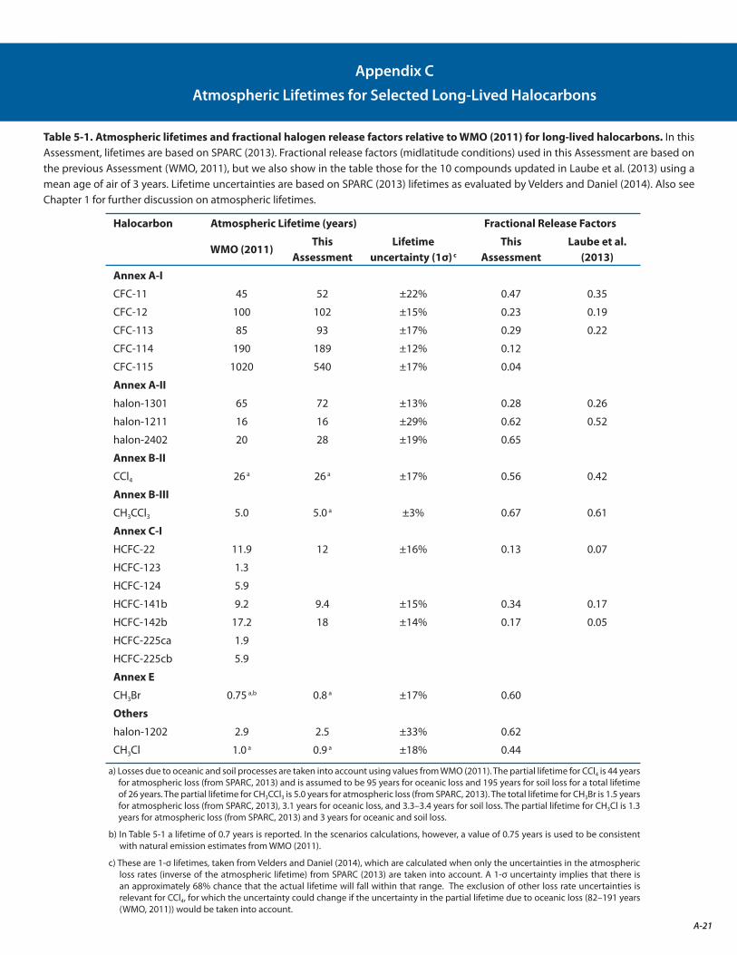
A-21
Table 5-1. Atmospheric lifetimes and fractional halogen release factors relative to WMO (2011) for long-lived halocarbons. In this Assessment, lifetimes are based on SPARC (2013). Fractional release factors (midlatitude conditions) used in this Assessment are based on the previous Assessment (WMO, 2011), but we also show in the table those for the 10 compounds updated in Laube et al. (2013) using a mean age of air of 3 years. Lifetime uncertainties are based on SPARC (2013) lifetimes as evaluated by Velders and Daniel (2014). Also see Chapter 1 for further discussion on atmospheric lifetimes.
Halocarbon Atmospheric Lifetime (years) Fractional Release Factors
WMO (2011)This
AssessmentLifetime
uncertainty (1σ) c
This Assessment
Laube et al. (2013)
Annex A-I
CFC-11 45 52 ±22% 0.47 0.35
CFC-12 100 102 ±15% 0.23 0.19
CFC-113 85 93 ±17% 0.29 0.22
CFC-114 190 189 ±12% 0.12
CFC-115 1020 540 ±17% 0.04
Annex A-II
halon-1301 65 72 ±13% 0.28 0.26
halon-1211 16 16 ±29% 0.62 0.52
halon-2402 20 28 ±19% 0.65
Annex B-II
CCl4 26 a 26 a ±17% 0.56 0.42
Annex B-III
CH3CCl3 5.0 5.0 a ±3% 0.67 0.61
Annex C-I
HCFC-22 11.9 12 ±16% 0.13 0.07
HCFC-123 1.3
HCFC-124 5.9
HCFC-141b 9.2 9.4 ±15% 0.34 0.17
HCFC-142b 17.2 18 ±14% 0.17 0.05
HCFC-225ca 1.9
HCFC-225cb 5.9
Annex E
CH3Br 0.75 a,b 0.8 a ±17% 0.60
Others
halon-1202 2.9 2.5 ±33% 0.62
CH3Cl 1.0 a 0.9 a ±18% 0.44
a) Losses due to oceanic and soil processes are taken into account using values from WMO (2011). The partial lifetime for CCl4 is 44 years for atmospheric loss (from SPARC, 2013) and is assumed to be 95 years for oceanic loss and 195 years for soil loss for a total lifetime of 26 years. The partial lifetime for CH3CCl3 is 5.0 years for atmospheric loss (from SPARC, 2013). The total lifetime for CH3Br is 1.5 years for atmospheric loss (from SPARC, 2013), 3.1 years for oceanic loss, and 3.3–3.4 years for soil loss. The partial lifetime for CH3Cl is 1.3 years for atmospheric loss (from SPARC, 2013) and 3 years for oceanic and soil loss.
b) In Table 5-1 a lifetime of 0.7 years is reported. In the scenarios calculations, however, a value of 0.75 years is used to be consistent with natural emission estimates from WMO (2011).
c) These are 1-σ lifetimes, taken from Velders and Daniel (2014), which are calculated when only the uncertainties in the atmospheric loss rates (inverse of the atmospheric lifetime) from SPARC (2013) are taken into account. A 1-σ uncertainty implies that there is an approximately 68% chance that the actual lifetime will fall within that range. The exclusion of other loss rate uncertainties is relevant for CCl4, for which the uncertainty could change if the uncertainty in the partial lifetime due to oceanic loss (82–191 years (WMO, 2011)) would be taken into account.
Appendix C
Atmospheric Lifetimes for Selected Long-Lived Halocarbons
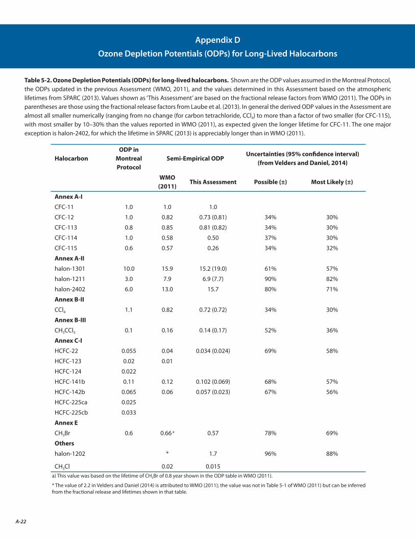
A-22
Table 5-2. Ozone Depletion Potentials (ODPs) for long-lived halocarbons. Shown are the ODP values assumed in the Montreal Protocol, the ODPs updated in the previous Assessment (WMO, 2011), and the values determined in this Assessment based on the atmospheric lifetimes from SPARC (2013). Values shown as ‘This Assessment’ are based on the fractional release factors from WMO (2011). The ODPs in parentheses are those using the fractional release factors from Laube et al. (2013). In general the derived ODP values in the Assessment are almost all smaller numerically (ranging from no change (for carbon tetrachloride, CCl4) to more than a factor of two smaller (for CFC-115), with most smaller by 10–30% than the values reported in WMO (2011), as expected given the longer lifetime for CFC-11. The one major exception is halon-2402, for which the lifetime in SPARC (2013) is appreciably longer than in WMO (2011).
HalocarbonODP in
Montreal Protocol
Semi-Empirical ODPUncertainties (95% confidence interval)
(from Velders and Daniel, 2014)
WMO (2011)
This Assessment Possible (±) Most Likely (±)
Annex A-I
CFC-11 1.0 1.0 1.0
CFC-12 1.0 0.82 0.73 (0.81) 34% 30%
CFC-113 0.8 0.85 0.81 (0.82) 34% 30%
CFC-114 1.0 0.58 0.50 37% 30%
CFC-115 0.6 0.57 0.26 34% 32%
Annex A-II
halon-1301 10.0 15.9 15.2 (19.0) 61% 57%
halon-1211 3.0 7.9 6.9 (7.7) 90% 82%
halon-2402 6.0 13.0 15.7 80% 71%
Annex B-II
CCl4 1.1 0.82 0.72 (0.72) 34% 30%
Annex B-III
CH3CCl3 0.1 0.16 0.14 (0.17) 52% 36%
Annex C-I
HCFC-22 0.055 0.04 0.034 (0.024) 69% 58%
HCFC-123 0.02 0.01
HCFC-124 0.022
HCFC-141b 0.11 0.12 0.102 (0.069) 68% 57%
HCFC-142b 0.065 0.06 0.057 (0.023) 67% 56%
HCFC-225ca 0.025
HCFC-225cb 0.033
Annex E
CH3Br 0.6 0.66 a 0.57 78% 69%
Others
halon-1202 * 1.7 96% 88%
CH3Cl 0.02 0.015a) This value was based on the lifetime of CH3Br of 0.8 year shown in the ODP table in WMO (2011).
* The value of 2.2 in Velders and Daniel (2014) is attributed to WMO (2011); the value was not in Table 5-1 of WMO (2011) but can be inferred from the fractional release and lifetimes shown in that table.
Appendix D
Ozone Depletion Potentials (ODPs) for Long-Lived Halocarbons
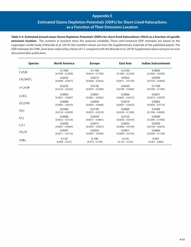
A-23
Table 5-4. Estimated annual-mean Ozone Depletion Potentials (ODPs) for short-lived halocarbons (VSLS) as a function of specific emissions location. The numbers in brackets show the seasonal variability. These semi-empirical ODP estimates are based on the Lagrangian model study of Brioude et al. (2010) (the numbers shown are from the Supplementary materials of the published paper). The ODP estimates for CHBr3 have been reduced by a factor of 3.1 compared with the Brioude et al. (2010) Supplement values owing to an error discovered after publication.
Species North America Europe East Asia Indian Subcontinent
C2H5Br 0.1300 [0.0780 – 0.2000]
0.1100[0.0610 – 0.1700]
0.2100[0.1000 – 0.3100]
0.4600[0.3400 – 0.6300]
CH2CBrCF30.0035
[0.0008 – 0.0077]0.0013
[0.0006 – 0.0024]0.0052
[0.0011 – 0.0130]0.0440
[0.0130 – 0.0830]
n-C3H7Br 0.0235 [0.0150 – 0.0320]
0.0150[0.0070 – 0.0260]
0.0420[0.0190 – 0.0600]
0.1700[0.0790 – 0.1300]
C2HCl30.0004
[0.0001 – 0.0007]0.0001
[0.0001 – 0.0002]0.0006
[0.0002 – 0.0013]0.0041
[0.0013 – 0.0079]
CCl3CHO 0.0008 [0.0005 – 0.0010]
0.0004[0.0002 – 0.0008]
0.0014[0.0007 – 0.0022]
0.0062[0.0026 – 0.0110]
CH3I 0.0360 [0.0130 – 0.0650]
0.0140[0.0072 – 0.0210]
0.0660[0.0220 – 0.1500]
0.4200[0.1300 – 0.8300]
CF3I 0.0068 [0.0022 – 0.0120]
0.0034[0.0013 – 0.0061]
0.0120[0.0020 – 0.0310]
0.0940[0.0290 – 0.1900]
C3F7I 0.0028 [0.0007 – 0.0064]
0.0015[0.0005 – 0.0031]
0.0033[0.0006 – 0.0100]
0.0390[0.0140 – 0.0670]
CH2ClI 0.0047 [0.0011 – 0.0110]
0.0024[0.0007 – 0.0050]
0.0051[0.0009 – 0.0150]
0.0660[0.0240 – 0.1100]
CHBr30.130
[0.094 – 0.201]0.106
[0.074 – 0.158]0.216
[0.123 – 0.310]0.581
[0.387 – 0.806]
Appendix E
Estimated Ozone Depletion Potentials (ODPs) for Short-Lived Halocarbons as a Function of Their Emissions Location
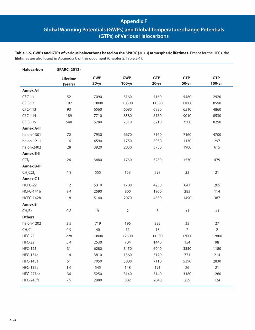
A-24
Table 5-5. GWPs and GTPs of various halocarbons based on the SPARC (2013) atmospheric lifetimes. Except for the HFCs, the lifetimes are also found in Appendix C of this document (Chapter 5, Table 5-1).
Halocarbon SPARC (2013)
Lifetime (years)
GWP20-yr
GWP100-yr
GTP20-yr
GTP50-yr
GTP100-yr
Annex A-I
CFC-11 52 7090 5160 7160 5480 2920
CFC-12 102 10800 10300 11300 11000 8590
CFC-113 93 6560 6080 6830 6510 4860
CFC-114 189 7710 8580 8180 9010 8530
CFC-115 540 5780 7310 6210 7500 8290
Annex A-II
halon-1301 72 7930 6670 8160 7160 4700
halon-1211 16 4590 1750 3950 1130 297
halon-2402 28 3920 2030 3730 1900 615
Annex B-II
CCl4 26 3480 1730 3280 1570 479
Annex B-III
CH3CCl3 4.8 555 153 298 32 21
Annex C-I
HCFC-22 12 5310 1780 4230 847 265
HCFC-141b 9.4 2590 800 1900 285 114
HCFC-142b 18 5140 2070 4530 1490 387
Annex E
CH3Br 0.8 9 2 3 <1 <1
Others
halon-1202 2.5 719 196 285 35 27
CH3Cl 0.9 40 11 13 2 2
HFC-23 228 10800 12500 11500 13000 12800
HFC-32 5.4 2530 704 1440 154 98
HFC-125 31 6280 3450 6040 3350 1180
HFC-134a 14 3810 1360 3170 771 214
HFC-143a 51 7050 5080 7110 5390 2830
HFC-152a 1.6 545 148 191 26 21
HFC-227ea 36 5250 3140 5140 3180 1260
HFC-245fa 7.9 2980 882 2040 259 124
Appendix F
Global Warming Potentials (GWPs) and Global Temperature change Potentials(GTPs) of Various Halocarbons
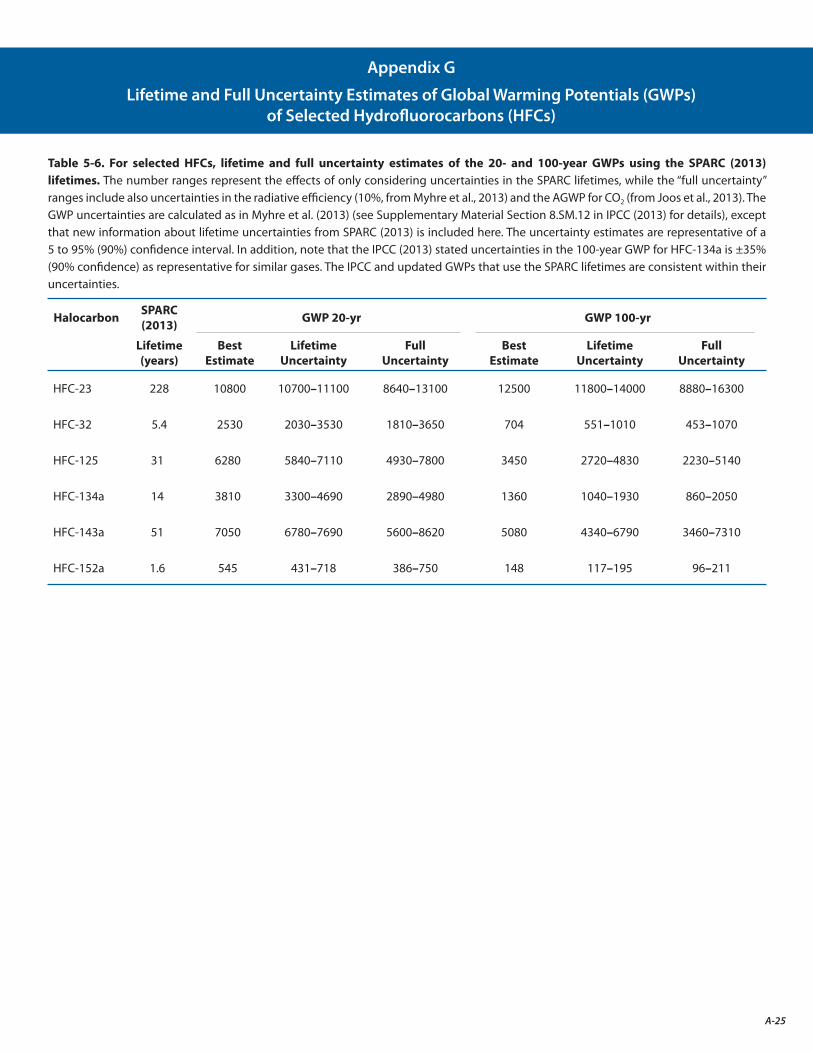
A-25
Table 5-6. For selected HFCs, lifetime and full uncertainty estimates of the 20- and 100-year GWPs using the SPARC (2013) lifetimes. The number ranges represent the effects of only considering uncertainties in the SPARC lifetimes, while the “full uncertainty” ranges include also uncertainties in the radiative efficiency (10%, from Myhre et al., 2013) and the AGWP for CO2 (from Joos et al., 2013). The GWP uncertainties are calculated as in Myhre et al. (2013) (see Supplementary Material Section 8.SM.12 in IPCC (2013) for details), except that new information about lifetime uncertainties from SPARC (2013) is included here. The uncertainty estimates are representative of a 5 to 95% (90%) confidence interval. In addition, note that the IPCC (2013) stated uncertainties in the 100-year GWP for HFC-134a is ±35% (90% confidence) as representative for similar gases. The IPCC and updated GWPs that use the SPARC lifetimes are consistent within their uncertainties.
Halocarbon SPARC(2013) GWP 20-yr GWP 100-yr
Lifetime (years)
Best Estimate
Lifetime Uncertainty
FullUncertainty
BestEstimate
Lifetime Uncertainty
FullUncertainty
HFC-23 228 10800 10700–11100 8640–13100 12500 11800–14000 8880–16300
HFC-32 5.4 2530 2030–3530 1810–3650 704 551–1010 453–1070
HFC-125 31 6280 5840–7110 4930–7800 3450 2720–4830 2230–5140
HFC-134a 14 3810 3300–4690 2890–4980 1360 1040–1930 860–2050
HFC-143a 51 7050 6780–7690 5600–8620 5080 4340–6790 3460–7310
HFC-152a 1.6 545 431–718 386–750 148 117–195 96–211
Appendix G
Lifetime and Full Uncertainty Estimates of Global Warming Potentials (GWPs)of Selected Hydrofluorocarbons (HFCs)
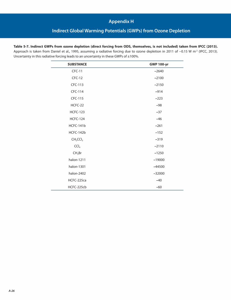
A-26
Table 5-7. Indirect GWPs from ozone depletion (direct forcing from ODS, themselves, is not included) taken from IPCC (2013). Approach is taken from Daniel et al., 1995, assuming a radiative forcing due to ozone depletion in 2011 of −0.15 W m-2 (IPCC, 2013). Uncertainty in this radiative forcing leads to an uncertainty in these GWPs of ±100%.
SUBSTANCE GWP 100-yr
CFC-11 –2640
CFC-12 –2100
CFC-113 –2150
CFC-114 –914
CFC-115 –223
HCFC-22 –98
HCFC-123 –37
HCFC-124 –46
HCFC-141b –261
HCFC-142b –152
CH3CCl3 –319
CCl4 –2110
CH3Br –1250
halon-1211 –19000
halon-1301 –44500
halon-2402 –32000
HCFC-225ca –40
HCFC-225cb –60
Appendix H
Indirect Global Warming Potentials (GWPs) from Ozone Depletion
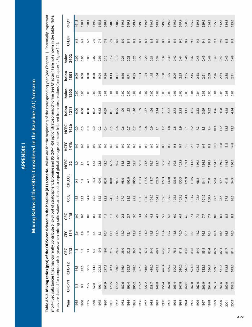
A-27
APP
END
IX I
Mix
ing
Ratio
s of
the
OD
Ss C
onsi
dere
d in
the
Base
line
(A1)
Sce
nari
o
Tabl
e A
5-2.
Mix
ing
rati
os (p
pt) o
f the
OD
Ss c
onsi
dere
d in
the
base
line
(A1)
sce
nari
o. V
alue
s ar
e fo
r the
beg
inni
ng o
f the
cor
resp
ondi
ng y
ear (
see
Chap
ter 1
). P
oten
tially
impo
rtan
t sh
ort-
lived
subs
tanc
es th
at m
ay c
urre
ntly
con
trib
ute
5 (2
–8) p
pt o
f str
atos
pher
ic b
rom
ine
and
95 (5
0–14
5) p
pt o
f str
atos
pher
ic c
hlor
ine
(see
Cha
pter
1) a
re n
ot sh
own
in th
e ta
ble.
Not
e:
Are
as a
re s
hade
d fo
r com
poun
ds in
yea
rs w
hen
mix
ing
ratio
val
ues
are
forc
ed to
equ
al g
loba
l ave
rage
est
imat
es in
ferr
ed fr
om o
bser
vatio
ns (s
ee C
hapt
er 1
, Fig
ure
1-1)
.
Year
CFC-
11CF
C-12
CFC-
113
CFC-
114
CFC-
115
CCl 4
CH3C
Cl3
HCF
C-22
HCF
C-14
1bH
CFC-
142b
halo
n12
11ha
lon
1202
halo
n13
01ha
lon
2402
CH3B
rCH
3Cl
1955
3.3
14.3
1.3
2.6
0.0
42.3
0.1
1.0
0.0
0.0
0.00
0.00
0.00
0.00
6.3
491.
3
1960
9.5
29.5
1.9
3.8
0.0
52.1
1.5
2.1
0.0
0.0
0.00
0.00
0.00
0.00
6.5
510.
3
1965
23.5
58.8
3.1
5.0
0.0
64.4
4.7
4.9
0.0
0.0
0.00
0.00
0.00
0.00
6.7
528.
1
1970
52.8
114.
35.
56.
50.
275
.916
.312
.10.
00.
00.
020.
000.
000.
027.
053
9.9
1975
106.
120
3.1
10.4
8.3
0.6
85.5
40.0
23.8
0.0
0.2
0.12
0.01
0.04
0.06
7.4
545.
8
1980
161.
929
7.1
19.0
10.7
1.5
92.9
82.0
42.5
0.0
0.4
0.69
0.01
0.36
0.15
7.8
548.
4
1981
170.
531
2.1
21.5
11.1
1.7
94.3
89.0
46.6
0.0
0.5
0.81
0.01
0.43
0.17
7.9
548.
6
1982
179.
233
0.5
24.5
11.6
2.0
95.7
94.1
50.7
0.0
0.6
0.95
0.01
0.51
0.19
8.0
548.
9
1983
187.
634
6.4
28.0
12.0
2.3
97.0
98.0
54.8
0.0
0.6
1.09
0.02
0.60
0.21
8.0
549.
1
1984
196.
436
3.7
32.2
12.4
2.7
98.5
102.
058
.80.
00.
71.
230.
020.
710.
238.
154
9.3
1985
206.
237
8.5
36.7
12.9
3.0
99.9
106.
562
.70.
00.
71.
400.
020.
850.
268.
254
9.4
1986
216.
239
7.9
41.8
13.4
3.4
101.
311
0.3
66.9
0.0
0.8
1.59
0.02
1.03
0.27
8.3
549.
5
1987
227.
241
6.4
47.5
14.0
3.9
103.
011
3.5
71.5
0.0
0.8
1.77
0.02
1.24
0.29
8.4
549.
6
1988
238.
743
9.0
54.0
14.5
4.3
104.
011
8.7
76.7
0.0
0.9
1.96
0.02
1.45
0.31
8.5
549.
7
1989
248.
845
9.3
60.9
15.0
4.7
104.
812
3.5
82.5
0.0
1.1
2.14
0.02
1.64
0.34
8.6
549.
8
1990
256.
447
6.4
67.6
15.4
5.2
105.
612
7.3
88.2
0.0
1.2
2.32
0.03
1.80
0.37
8.7
549.
8
1991
262.
048
9.7
73.3
15.7
5.6
105.
913
0.8
93.7
0.0
1.8
2.52
0.03
1.95
0.39
8.8
549.
9
1992
265.
450
0.7
78.2
15.8
6.0
105.
813
3.6
99.8
0.1
2.8
2.72
0.03
2.09
0.42
8.9
549.
9
1993
267.
851
0.0
81.2
16.0
6.4
105.
313
0.3
103.
90.
43.
92.
920.
032.
230.
449.
054
9.9
1994
268.
151
6.5
83.0
16.1
6.8
104.
412
1.9
109.
11.
55.
13.
110.
032.
350.
469.
255
0.0
1995
267.
852
3.0
83.8
16.1
7.1
103.
711
0.5
113.
62.
86.
23.
350.
042.
450.
479.
255
5.2
1996
267.
052
8.7
84.0
16.2
7.4
102.
698
.211
9.4
4.5
7.2
3.53
0.04
2.53
0.48
9.2
539.
3
1997
266.
053
2.9
83.8
16.3
7.7
101.
684
.112
4.2
6.4
8.3
3.69
0.05
2.61
0.49
9.1
529.
6
1998
264.
653
6.4
83.4
16.4
7.9
100.
771
.012
8.9
8.2
9.4
3.82
0.05
2.69
0.49
9.3
554.
3
1999
263.
353
9.3
82.9
16.4
8.0
99.6
59.4
134.
310
.110
.43.
960.
042.
760.
499.
355
5.5
2000
261.
654
1.4
82.3
16.5
8.1
98.5
49.7
139.
211
.811
.44.
080.
042.
840.
499.
054
2.8
2001
260.
054
2.8
81.7
16.5
8.2
97.5
41.5
144.
713
.512
.54.
180.
032.
880.
498.
553
4.8
2002
258.
254
3.6
81.1
16.6
8.3
96.5
34.5
150.
514
.813
.34.
240.
022.
910.
498.
353
3.6
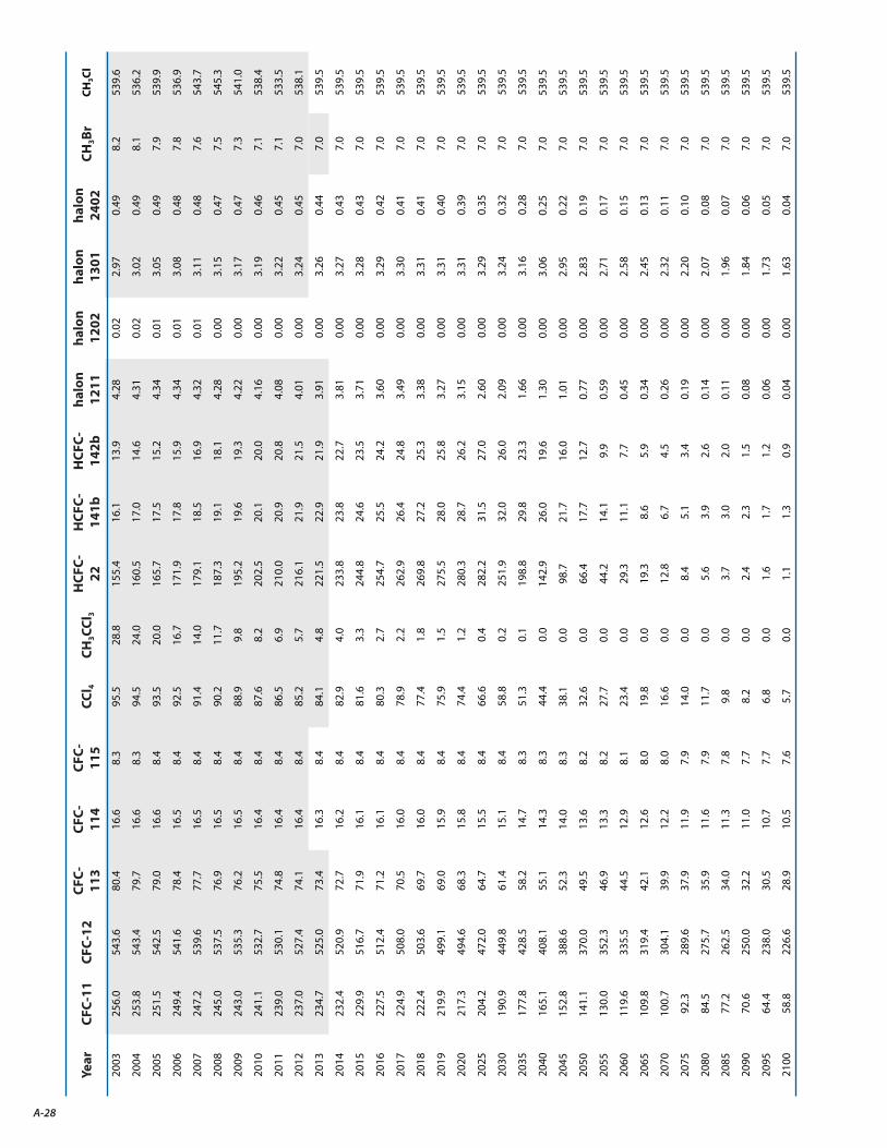
A-28
Year
CFC-
11CF
C-12
CFC-
113
CFC-
114
CFC-
115
CCl 4
CH3C
Cl3
HCF
C-22
HCF
C-14
1bH
CFC-
142b
halo
n12
11ha
lon
1202
halo
n13
01ha
lon
2402
CH3B
rCH
3Cl
2003
256.
054
3.6
80.4
16.6
8.3
95.5
28.8
155.
416
.113
.94.
280.
022.
970.
498.
253
9.6
2004
253.
854
3.4
79.7
16.6
8.3
94.5
24.0
160.
517
.014
.64.
310.
023.
020.
498.
153
6.2
2005
251.
554
2.5
79.0
16.6
8.4
93.5
20.0
165.
717
.515
.24.
340.
013.
050.
497.
953
9.9
2006
249.
454
1.6
78.4
16.5
8.4
92.5
16.7
171.
917
.815
.94.
340.
013.
080.
487.
853
6.9
2007
247.
253
9.6
77.7
16.5
8.4
91.4
14.0
179.
118
.516
.94.
320.
013.
110.
487.
654
3.7
2008
245.
053
7.5
76.9
16.5
8.4
90.2
11.7
187.
319
.118
.14.
280.
003.
150.
477.
554
5.3
2009
243.
053
5.3
76.2
16.5
8.4
88.9
9.8
195.
219
.619
.34.
220.
003.
170.
477.
354
1.0
2010
241.
153
2.7
75.5
16.4
8.4
87.6
8.2
202.
520
.120
.04.
160.
003.
190.
467.
153
8.4
2011
239.
053
0.1
74.8
16.4
8.4
86.5
6.9
210.
020
.920
.84.
080.
003.
220.
457.
153
3.5
2012
237.
052
7.4
74.1
16.4
8.4
85.2
5.7
216.
121
.921
.54.
010.
003.
240.
457.
053
8.1
2013
234.
752
5.0
73.4
16.3
8.4
84.1
4.8
221.
522
.921
.93.
910.
003.
260.
447.
053
9.5
2014
232.
452
0.9
72.7
16.2
8.4
82.9
4.0
233.
823
.822
.73.
810.
003.
270.
437.
053
9.5
2015
229.
951
6.7
71.9
16.1
8.4
81.6
3.3
244.
824
.623
.53.
710.
003.
280.
437.
053
9.5
2016
227.
551
2.4
71.2
16.1
8.4
80.3
2.7
254.
725
.524
.23.
600.
003.
290.
427.
053
9.5
2017
224.
950
8.0
70.5
16.0
8.4
78.9
2.2
262.
926
.424
.83.
490.
003.
300.
417.
053
9.5
2018
222.
450
3.6
69.7
16.0
8.4
77.4
1.8
269.
827
.225
.33.
380.
003.
310.
417.
053
9.5
2019
219.
949
9.1
69.0
15.9
8.4
75.9
1.5
275.
528
.025
.83.
270.
003.
310.
407.
053
9.5
2020
217.
349
4.6
68.3
15.8
8.4
74.4
1.2
280.
328
.726
.23.
150.
003.
310.
397.
053
9.5
2025
204.
247
2.0
64.7
15.5
8.4
66.6
0.4
282.
231
.527
.02.
600.
003.
290.
357.
053
9.5
2030
190.
944
9.8
61.4
15.1
8.4
58.8
0.2
251.
932
.026
.02.
090.
003.
240.
327.
053
9.5
2035
177.
842
8.5
58.2
14.7
8.3
51.3
0.1
198.
829
.823
.31.
660.
003.
160.
287.
053
9.5
2040
165.
140
8.1
55.1
14.3
8.3
44.4
0.0
142.
926
.019
.61.
300.
003.
060.
257.
053
9.5
2045
152.
838
8.6
52.3
14.0
8.3
38.1
0.0
98.7
21.7
16.0
1.01
0.00
2.95
0.22
7.0
539.
5
2050
141.
137
0.0
49.5
13.6
8.2
32.6
0.0
66.4
17.7
12.7
0.77
0.00
2.83
0.19
7.0
539.
5
2055
130.
035
2.3
46.9
13.3
8.2
27.7
0.0
44.2
14.1
9.9
0.59
0.00
2.71
0.17
7.0
539.
5
2060
119.
633
5.5
44.5
12.9
8.1
23.4
0.0
29.3
11.1
7.7
0.45
0.00
2.58
0.15
7.0
539.
5
2065
109.
831
9.4
42.1
12.6
8.0
19.8
0.0
19.3
8.6
5.9
0.34
0.00
2.45
0.13
7.0
539.
5
2070
100.
730
4.1
39.9
12.2
8.0
16.6
0.0
12.8
6.7
4.5
0.26
0.00
2.32
0.11
7.0
539.
5
2075
92.3
289.
637
.911
.97.
914
.00.
08.
45.
13.
40.
190.
002.
200.
107.
053
9.5
2080
84.5
275.
735
.911
.67.
911
.70.
05.
63.
92.
60.
140.
002.
070.
087.
053
9.5
2085
77.2
262.
534
.011
.37.
89.
80.
03.
73.
02.
00.
110.
001.
960.
077.
053
9.5
2090
70.6
250.
032
.211
.07.
78.
20.
02.
42.
31.
50.
080.
001.
840.
067.
053
9.5
2095
64.4
238.
030
.510
.77.
76.
80.
01.
61.
71.
20.
060.
001.
730.
057.
053
9.5
2100
58.8
226.
628
.910
.57.
65.
70.
01.
11.
30.
90.
040.
001.
630.
047.
053
9.5
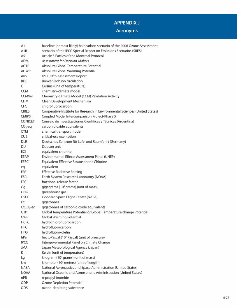
A-29
APPENDIX J
Acronyms
A1 baseline (or most likely) halocarbon scenario of the 2006 Ozone AssessmentA1B scenario of the IPCC Special Report on Emissions Scenarios (SRES)A5 Article 5 Parties of the Montreal ProtocolADM Assessment for Decision-MakersAGTP Absolute Global Temperature PotentialAGWP Absolute Global Warming PotentialAR5 IPCC Fifth Assessment Report BDC Brewer-Dobson circulationC Celsius (unit of temperature)CCM chemistry-climate modelCCMVal Chemistry-Climate Model (CCM) Validation ActivityCDM Clean Development MechanismCFC chlorofluorocarbonCIRES Cooperative Institute for Research in Environmental Sciences (United States)CMIP5 Coupled Model Intercomparison Project-Phase 5 CONICET Consejo de Investigaciones Cientificas y Técnicas (Argentina)CO2-eq carbon dioxide equivalentsCTM chemical transport modelCUE critical-use exemptionDLR Deutsches Zentrum für Luft- und Raumfahrt (Germany)DU Dobson unitECl equivalent chlorineEEAP Environmental Effects Assessment Panel (UNEP)EESC Equivalent Effective Stratospheric Chlorineeq equivalentERF Effective Radiative ForcingESRL Earth System Research Laboratory (NOAA)FRF fractional release factorGg gigagrams (109 grams) (unit of mass)GHG greenhouse gasGSFC Goddard Space Flight Center (NASA)Gt gigatonnesGtCO2-eq gigatonnes of carbon dioxide equivalentsGTP Global Temperature Potential or Global Temperature change PotentialGWP Global Warming PotentialHCFC hydrochlorofluorocarbonHFC hydrofluorocarbonHFO hydrofluoro-olefinhPa hectoPascal (102 Pascal) (unit of pressure)IPCC Intergovernmental Panel on Climate Change JMA Japan Meteorological Agency (Japan)K Kelvin (unit of temperature)kg kilogram (103 grams) (unit of mass)km kilometer (103 meters) (unit of length)NASA National Aeronautics and Space Administration (United States)NOAA National Oceanic and Atmospheric Administration (United States)nPB n-propyl bromideODP Ozone Depletion PotentialODS ozone-depleting substance
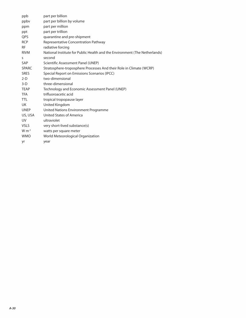
A-30
ppb part per billionppbv part per billion by volumeppm part per millionppt part per trillionQPS quarantine and pre-shipmentRCP Representative Concentration PathwayRF radiative forcingRIVM National Institute for Public Health and the Environment (The Netherlands)s secondSAP Scientific Assessment Panel (UNEP)SPARC Stratosphere-troposphere Processes And their Role in Climate (WCRP)SRES Special Report on Emissions Scenarios (IPCC)2-D two-dimensional3-D three-dimensionalTEAP Technology and Economic Assessment Panel (UNEP)TFA trifluoroacetic acidTTL tropical tropopause layerUK United KingdomUNEP United Nations Environment ProgrammeUS, USA United States of AmericaUV ultravioletVSLS very short-lived substance(s)W m-2 watts per square meterWMO World Meteorological Organizationyr year
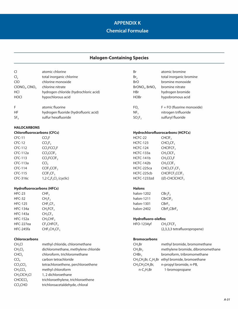
A-31
Halogen-Containing Species
Cl atomic chlorine Br atomic bromineCly total inorganic chlorine Bry total inorganic bromineClO chlorine monoxide BrO bromine monoxideClONO2, ClNO3 chlorine nitrate BrONO2, BrNO3 bromine nitrateHCl hydrogen chloride (hydrochloric acid) HBr hydrogen bromideHOCl hypochlorous acid HOBr hypobromous acid
F atomic fluorine FOx F + FO (fluorine monoxide)HF hydrogen fluoride (hydrofluoric acid) NF3 nitrogen trifluorideSF6 sulfur hexafluoride SO2F2 sulfuryl fluoride
HALOCARBONSChlorofluorocarbons (CFCs) Hydrochlorofluorocarbons (HCFCs)CFC-11 CCl3F HCFC-22 CHClF2
CFC-12 CCl2F2 HCFC-123 CHCl2CF3
CFC-112 CCl2FCCl2F HCFC-124 CHClFCF3
CFC-112a CCl3CClF2 HCFC-133a CH2ClCF3
CFC-113 CCl2FCClF2 HCFC-141b CH3CCl2FCFC-113a CCl3 HCFC-142b CH3CClF2
CFC-114 CClF2CClF2 HCFC-225ca CHCl2CF2CF3
CFC-115 CClF2CF3 HCFC-225cb CHClFCF2CClF2
CFC-316c 1,2 C4F6Cl2 (cyclic) HCFC-1233zd ((E)-CHClCHCF3
Hydrofluorocarbons (HFCs) HalonsHFC-23 CHF3 halon-1202 CBr2F2
HFC-32 CH2F2 halon-1211 CBrClF2
HFC-125 CHF2CF3 halon-1301 CBrF3
HFC-134a CH2FCF3 halon-2402 CBrF2CBrF2
HFC-143a CH3CF3 HFC-152a CH3CHF2 Hydrofluoro-olefinsHFC-227ea CF3CHFCF3 HFO-1234yf CH2CFCF3
HFC-245fa CHF2CH2CF3 (2,3,3,3 tetrafluoropropene)
Chlorocarbons BromocarbonsCH3Cl methyl chloride, chloromethane CH3Br methyl bromide, bromomethaneCH2Cl2 dichloromethane, methylene chloride CH2Br2 methylene bromide, dibromomethaneCHCl3 chloroform, trichloromethane CHBr3 bromoform, tribromomethaneCCl4 carbon tetrachloride CH3CH2Br, C2H5Br ethyl bromide, bromoethaneCCl2CCl2 tetrachloroethene, perchloroethene CH3CH2CH2Br, n-propyl bromide, n-PB, CH3CCl3 methyl chloroform n-C3H7Br 1-bromopropaneCH2ClCH2Cl 1, 2 dichloroethaneCHClCCl2 trichloroethylene, trichloroetheneCCl3CHO trichloroacetaldehyde, chloral
APPENDIX K
Chemical Formulae
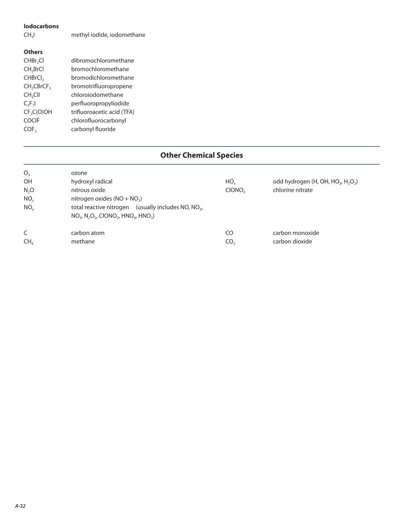
A-32
IodocarbonsCH3I methyl iodide, iodomethane
OthersCHBr2Cl dibromochloromethaneCH2BrCl bromochloromethaneCHBrCl2 bromodichloromethaneCH2CBrCF3 bromotrifluoropropeneCH2ClI chloroiodomethane C3F7I perfluoropropyliodideCF3C(O)OH trifluoroacetic acid (TFA)COClF chlorofluorocarbonylCOF2 carbonyl fluoride
Other Chemical Species O3 ozone OH hydroxyl radical HOx odd hydrogen (H, OH, HO2, H2O2)N2O nitrous oxide ClONO2 chlorine nitrateNOx nitrogen oxides (NO + NO2)NOy total reactive nitrogen (usually includes NO, NO2, NO3, N2O5, ClONO2, HNO4, HNO3)
C carbon atom CO carbon monoxideCH4 methane CO2 carbon dioxide