
Faculte de genieGenie electrique et genie informatique
Auditory System for a Mobile Robot
These de doctoratSpecialite : genie electrique
Jean-Marc VALIN
Sherbrooke (Quebec) Canada 10 aout 2005


i
Abstract
The auditory system of living creatures provides useful information about the world, such as
the location and interpretation of sound sources. For humans, it means to be able to focus one’s
attention on events, such as a phone ringing, a vehicle honking, a person taking, etc. For those
who do not suffer from hearing impairments, it is hard to imagine a day without being able to
hear, especially in a very dynamic and unpredictable world. Mobile robots would also benefit
greatly from having auditory capabilities.
In this thesis, we propose an artificial auditory system that gives a robot the ability to locate
and track sounds, as well as to separate simultaneous sound sources and recognising simulta-
neous speech. We demonstrate that it is possible to implement these capabilities using an array
of microphones, without trying to imitate the human auditory system. The sound source lo-
calisation and tracking algorithm uses a steered beamformer to locate sources, which are then
tracked using a multi-source particle filter. Separation of simultaneous sound sources is achieved
using a variant of the Geometric Source Separation (GSS) algorithm, combined with a multi-
source post-filter that further reduces noise, interference and reverberation. Speech recognition
is performed on separated sources, either directly or by using Missing Feature Theory (MFT) to
estimate the reliability of the speech features.
The results obtained show that it is possible to track up to four simultaneous sound sources,
even in noisy and reverberant environments. Real-time control of the robot following a sound
source is also demonstrated. The sound source separation approach we propose is able to
achieve a 13.7 dB improvement in signal-to-noise ratio compared to a single microphone when
three speakers are present. In these conditions, the system demonstrates more than 80% accu-
racy on digit recognition, higher than most human listeners could obtain in our small case study
when recognising only one of these sources. All these new capabilities will allow humans to
interact more naturally with a mobile robot in real life settings.

ii

iii
Sommaire
La plupart des êtres vivants possèdent un système auditif leur fournissant de l’information
utile sur leur environnement, comme la direction et l’interprétation des source sonores. Cela
permet de diriger notre attention sur des événements, comme une sonnerie de téléphone, le
klaxon d’un véhicule, une personne qui parle, etc. Pour ceux qui ne souffrent pas d’un problème
auditif, il est difficile d’imaginer passer une journée sans pouvoir entendre, particulièrement
dans un environnement dynamique et imprévisible. Les robots mobiles pourraient eux aussi
tirer un bénéfice important de capacités auditives.
Dans cette thèse, nous proposons un système d’audition artificielle dotant un robot de la
capacité de localiser et suivre des sons, ainsi que de la capacité de séparer des sources sonores
sonores simultanées et de reconnaître ce qui est dit. Nous démontrons qu’il est possible de
réaliser ces capacités à l’aide d’un réseau de microphones, sans la nécessité d’imiter le système
auditif humain. L’algorithme de localisation et suivi de sources sonores utilise un beamformer
dirigé pour localiser les sources, qui sont ensuite suivies en utilisant un filtre particulaire. La sé-
paration de sources sonores simultanées est accomplie par une variante de l’algorithme de sépa-
ration géometrique des sources (Geometric Source Separation), combinée à un post-traitement
multi-source permettant de réduire le bruit, les interférences et la réverbération. Les sources
séparées sont ensuite utilisées pour effectuer la reconnaissance vocale, soit directement, soit en
utilisant la théorie des données manquantes (Missing Feature Theory) qui tient compte de la
fiabilité des paramètres de la parole séparée.
Les résultats obtenus montrent qu’il est possible de suivre jusqu’à quatre sources sonores
simultanées, même dans des environnements bruités et réverbérants. Nous démontrons aussi
le contrôle en temps réel d’un robot se déplaçant pour suivre une source en mouvement. De
plus, lorsque trois personnes parlent en même temps, l’approche proposée pour la séparation
des sources sonores permet d’améliorer de 13.7 dB le rapport signal-à-bruit si on compare à
l’utilisation d’un seul microphone. Dans ces conditions, le système obtient un taux de recon-
naissance supérieur à 80% sur des chiffres, ce qui est supérieur à ce que la plupart des auditeurs
humains ont obtenu lors de tests simples de reconnaissance sur une seule de ces sources. Ces
nouvelles capacités auditives permettront aux humains d’interagir de façon plus naturelle avec
un robot mobile.

iv

v
Acknowledgements
I would like to express my gratitude to my thesis supervisor François Michaud and my thesis
co-supervisor Jean Rouat for their support and feedback during the course of this thesis. Their
knowledge and insight have greatly contributed to the success of this project.
During this research, I was supported financially by the National Science and Engineering
Research Council of Canada (NSERC), the Quebec Fonds de recherche sur la nature et les
technologies (FQRNT) and the Université de Sherbrooke. François Michaud holds the Canada
Research Chair (CRC) in Mobile Robotics and Autonomous Intelligent Systems. This research
is supported financially by the CRC Program and the Canadian Foundation for Innovation (CFI).
I would like to thank Hiroshi G. Okuno for receiving me at the Kyoto University Speech
Media Processing Group for an internship from August to November 2004, during which I was
introduced to the missing feature theory. During this stay, I was supported financially by the
Japan Society for the Promotion of Science (JSPS) short-term exchange student scholarship.
Special thanks to Brahim Hadjou for help formalising the particle filtering notation, to Do-
minic Létourneau and Pierre Lepage for implementing what was necessary to control the robot
in real time using my algorithms and to Yannick Brosseau for performing speech recognition
experiments. Thanks to Serge Caron and Jonathan Bisson for the design and fabrication of the
microphones. Many thanks to everyone at the Mobile Robotics and Intelligent Systems Re-
search Laboratory (LABORIUS) who took part in my numerous experiments. I would like to
thank Nuance Corporation for providing us with a free license to use its Nuance Voice Platform.
I am grateful to my wife, Nathalie, for her love, encouragement and unconditional support
throughout my PhD, and to my son, Alexandre, for giving me a reason to finish on schedule!

vi

Contents
1 Overview of the Thesis 1
1.1 Audition in Mobile Robotics . . . . . . . . . . . . . . . . . . . . . . . . . . . 4
1.2 Experimental Setup . . . . . . . . . . . . . . . . . . . . . . . . . . . . . . . . 6
1.3 Thesis Outline . . . . . . . . . . . . . . . . . . . . . . . . . . . . . . . . . . . 8
2 Sound Source Localisation 11
2.1 Related Work . . . . . . . . . . . . . . . . . . . . . . . . . . . . . . . . . . . 12
2.2 System Overview . . . . . . . . . . . . . . . . . . . . . . . . . . . . . . . . . 13
2.3 Localisation Using a Steered Beamformer . . . . . . . . . . . . . . . . . . . . 14
2.3.1 Delay-And-Sum Beamformer . . . . . . . . . . . . . . . . . . . . . . 15
2.3.2 Spectral Weighting . . . . . . . . . . . . . . . . . . . . . . . . . . . . 17
2.3.3 Direction Search on a Spherical Grid . . . . . . . . . . . . . . . . . . 18
2.3.4 Direction Refining . . . . . . . . . . . . . . . . . . . . . . . . . . . . 21
2.4 Particle-Based Tracking . . . . . . . . . . . . . . . . . . . . . . . . . . . . . . 22
2.4.1 Prediction . . . . . . . . . . . . . . . . . . . . . . . . . . . . . . . . . 24
2.4.2 Instantaneous Direction Probabilities from Beamformer Response . . . 25
2.4.3 Probabilities for Multiple Sources . . . . . . . . . . . . . . . . . . . . 27
2.4.4 Weight Update . . . . . . . . . . . . . . . . . . . . . . . . . . . . . . 30
2.4.5 Adding or Removing Sources . . . . . . . . . . . . . . . . . . . . . . 31
2.4.6 Parameter Estimation . . . . . . . . . . . . . . . . . . . . . . . . . . . 32
vii

viii CONTENTS
2.4.7 Resampling . . . . . . . . . . . . . . . . . . . . . . . . . . . . . . . . 33
2.5 Results . . . . . . . . . . . . . . . . . . . . . . . . . . . . . . . . . . . . . . . 33
2.5.1 Characterisation . . . . . . . . . . . . . . . . . . . . . . . . . . . . . 34
2.5.1.1 Detection Reliability . . . . . . . . . . . . . . . . . . . . . . 34
2.5.1.2 Localisation Accuracy . . . . . . . . . . . . . . . . . . . . . 35
2.5.2 Source Tracking . . . . . . . . . . . . . . . . . . . . . . . . . . . . . 36
2.5.2.1 Moving Sources . . . . . . . . . . . . . . . . . . . . . . . . 36
2.5.2.2 Moving Robot . . . . . . . . . . . . . . . . . . . . . . . . . 37
2.5.2.3 Sources with Intersecting Trajectories . . . . . . . . . . . . 37
2.5.2.4 Number of Microphones . . . . . . . . . . . . . . . . . . . . 38
2.5.2.5 Audio Bandwidth . . . . . . . . . . . . . . . . . . . . . . . 40
2.5.3 Localisation and Tracking for Robot Control . . . . . . . . . . . . . . 40
2.6 Discussion . . . . . . . . . . . . . . . . . . . . . . . . . . . . . . . . . . . . . 41
3 Sound Source Separation 43
3.1 Related Work . . . . . . . . . . . . . . . . . . . . . . . . . . . . . . . . . . . 44
3.2 System Overview . . . . . . . . . . . . . . . . . . . . . . . . . . . . . . . . . 46
3.3 Linear Source Separation . . . . . . . . . . . . . . . . . . . . . . . . . . . . . 47
3.3.1 Geometric Source Separation . . . . . . . . . . . . . . . . . . . . . . 47
3.3.2 Proposed Improvements to the GSS algorithm . . . . . . . . . . . . . . 49
3.3.2.1 Stochastic Gradient Adaptation . . . . . . . . . . . . . . . . 49
3.3.2.2 Regularisation Term . . . . . . . . . . . . . . . . . . . . . . 50
3.3.3 Initialisation . . . . . . . . . . . . . . . . . . . . . . . . . . . . . . . 50
3.4 Multi-Source Post-Filter . . . . . . . . . . . . . . . . . . . . . . . . . . . . . 51
3.4.1 Noise Estimation . . . . . . . . . . . . . . . . . . . . . . . . . . . . . 52
3.4.2 Suppression Rule in the Presence of Speech . . . . . . . . . . . . . . . 53
3.4.3 Optimal Gain Modification Under Speech Presence Uncertainty . . . . 55
3.4.4 Post-filter Initialisation . . . . . . . . . . . . . . . . . . . . . . . . . . 56

CONTENTS ix
3.5 Results . . . . . . . . . . . . . . . . . . . . . . . . . . . . . . . . . . . . . . . 57
3.6 Discussion . . . . . . . . . . . . . . . . . . . . . . . . . . . . . . . . . . . . . 60
4 Speech Recognition of Separated Sound Sources 65
4.1 Related Work in Robust Speech Recognition . . . . . . . . . . . . . . . . . . . 66
4.1.1 Missing Feature Theory Overview . . . . . . . . . . . . . . . . . . . . 67
4.1.2 Applications of Missing Feature Theory . . . . . . . . . . . . . . . . . 68
4.2 ASR on Separated Sources . . . . . . . . . . . . . . . . . . . . . . . . . . . . 69
4.3 Missing Feature Recognition . . . . . . . . . . . . . . . . . . . . . . . . . . . 71
4.3.1 Computation of Missing Feature Masks . . . . . . . . . . . . . . . . . 71
4.3.2 Speech Analysis for Missing Feature ASR . . . . . . . . . . . . . . . . 73
4.3.3 Automatic Speech Recognition Using Missing Feature Theory . . . . . 74
4.4 Results . . . . . . . . . . . . . . . . . . . . . . . . . . . . . . . . . . . . . . . 74
4.4.1 Direct Coupling . . . . . . . . . . . . . . . . . . . . . . . . . . . . . . 75
4.4.1.1 Human Capabilities . . . . . . . . . . . . . . . . . . . . . . 76
4.4.1.2 Moving Sources . . . . . . . . . . . . . . . . . . . . . . . . 78
4.4.2 Missing Feature Theory Coupling . . . . . . . . . . . . . . . . . . . . 79
4.4.2.1 Separated Signals . . . . . . . . . . . . . . . . . . . . . . . 80
4.4.2.2 Speech Recognition Accuracy . . . . . . . . . . . . . . . . . 81
4.5 Discussion . . . . . . . . . . . . . . . . . . . . . . . . . . . . . . . . . . . . . 82
5 Conclusion 87
5.1 Future Work . . . . . . . . . . . . . . . . . . . . . . . . . . . . . . . . . . . . 89
5.2 Perspectives . . . . . . . . . . . . . . . . . . . . . . . . . . . . . . . . . . . . 90

x CONTENTS

List of Figures
1.1 Microphones used on the Spartacus robot. . . . . . . . . . . . . . . . . . . . . 7
1.2 Spartacus robot in configurations. . . . . . . . . . . . . . . . . . . . . . . . . 8
1.3 Overview of the proposed artificial auditory system. . . . . . . . . . . . . . . . 9
2.1 Overview of the Localisation subsystem. . . . . . . . . . . . . . . . . . . . . . 14
2.2 Recursive subdivision of a triangular element. . . . . . . . . . . . . . . . . . . 19
2.3 TDOA for the far field approximation. . . . . . . . . . . . . . . . . . . . . . . 20
2.4 Probabilistic tracking of multiple sources using a fixed grid. . . . . . . . . . . 23
2.5 Example of two sources being represented by a particle filter. . . . . . . . . . . 24
2.6 Beamformer output probabilities Pq for azimuth as a function of time. . . . . . 26
2.7 Assignment example where two of the tracked sources are observed, with one
new source and one false detection. . . . . . . . . . . . . . . . . . . . . . . . . 27
2.8 Tracking of four moving sources, showing azimuth as a function of time. . . . . 32
2.9 Source trajectories (robot represented as an X, sources represented with dots). . 36
2.10 Four speakers moving around a stationary robot. False detection shown in black. 37
2.11 Two stationary speakers with the robot moving. False detection shown in black. 38
2.12 Two speakers intersecting in front of the robot. . . . . . . . . . . . . . . . . . 38
2.13 Tracking of four sources using C2 in the E1 environment, using 4 to 7 micro-
phones. . . . . . . . . . . . . . . . . . . . . . . . . . . . . . . . . . . . . . . 39
xi

xii LIST OF FIGURES
2.14 Tracking of four sources using C2 in the E1 environment for reduced audio
bandwidth. . . . . . . . . . . . . . . . . . . . . . . . . . . . . . . . . . . . . 40
3.1 Overview of the separation system. . . . . . . . . . . . . . . . . . . . . . . . . 46
3.2 Overview of the complete separation system. . . . . . . . . . . . . . . . . . . 52
3.3 Signal-to-noise ratio (SNR) and log-spectral distortion (LSD) for each source
of interest. . . . . . . . . . . . . . . . . . . . . . . . . . . . . . . . . . . . . . 59
3.4 Attenuation of noise and interference in the direction of each source of interest. 60
3.5 Temporal signals for separation of first source. . . . . . . . . . . . . . . . . . . 62
3.6 Spectrograms for separation of first source comparing different processing. . . 63
4.1 Direct integration of speech recognition. . . . . . . . . . . . . . . . . . . . . . 69
4.2 Speech recognition integration using missing feature theory . . . . . . . . . . . 70
4.3 Speech recognition results for two simultaneous speakers. . . . . . . . . . . . . 76
4.4 Speech recognition results for three simultaneous speakers. . . . . . . . . . . . 77
4.5 Human versus machine speech recognition accuracy. . . . . . . . . . . . . . . 78
4.6 Source trajectories (azimuth as a function of time): recognition on two moving
speakers. . . . . . . . . . . . . . . . . . . . . . . . . . . . . . . . . . . . . . . 79
4.7 SIG 2 robot with eight microphones (two are occluded). . . . . . . . . . . . . . 80
4.8 Missing feature masks for separation of three speakers. . . . . . . . . . . . . . 81
4.9 Speech recognition accuracy results for 30◦ separation between speakers. . . . 83
4.10 Speech recognition accuracy results for 60◦ separation between speakers. . . . 84
4.11 Speech recognition accuracy results for 90◦ separation between speakers. . . . 85

List of Tables
2.1 Detection reliability for C1 and C2 configurations. . . . . . . . . . . . . . . . . 35
2.2 Correct localisation rate as a function of sound type and distance for C2 config-
uration. . . . . . . . . . . . . . . . . . . . . . . . . . . . . . . . . . . . . . . 35
2.3 Localisation accuracy (root mean square error). . . . . . . . . . . . . . . . . . 36
xiii

xiv LIST OF TABLES

List of Algorithms
1 Steered beamformer direction search. . . . . . . . . . . . . . . . . . . . . . . 19
2 Localisation of multiple sources. . . . . . . . . . . . . . . . . . . . . . . . . . 21
3 Particle-based tracking algorithm . . . . . . . . . . . . . . . . . . . . . . . . . 24
xv

xvi LIST OF ALGORITHMS

Lexicon
ASR. Automatic Speech Recognition.
CMS. Cepstral Mean Subtraction (also cepstral mean normalisation).
DCT. Discrete Cosine Transform.
DSP. Digital Signal Processor.
FFT. Fast Fourier Transform.
GSS. Geometric Source Separation.
LSS. Linear Source Separation.
MCRA. Minima-Controlled Recursive Average.
MFCC. Mel-Frequency Cepstral Coefficient.
MFT. Missing Feature Theory.
MMSE. Minimum Mean Square Error.
pdf. Probability density function.
Reverberation Time (T60). Time for reverberation to decrease by 60 dB.
SNR. Signal-to-Noise Ratio.
SRR. Signal-to-Reverberant Ratio.
TDOA. Time Delay of Arrival.
xvii

xviii LIST OF ALGORITHMS

Chapter 1
Overview of the Thesis
The auditory system of living creatures provides significant information about the world, such
as the location and the interpretation of sound sources. For humans, it means to be able to focus
one’s attention on events, such as a phone ringing, a vehicle honking, a person taking, etc. For
those who do not suffer from hearing impairments, it is hard to imagine a day without being
able to hear, especially in a very dynamic and unpredictable world.
Brooks et al. [1] postulate that the essence of intelligence lies in four main aspects: de-
velopment, social interaction, embodiment, and integration. It turns out that hearing plays a
role in three of these factors. Obviously, speech is by far the preferred means of commu-
nication between humans. Hearing also plays a very important role in human development.
Marschark [2] even suggests that although deaf children have similar IQ results compared to
other children, they do experience more learning difficulties in school. Hearing is useful for the
integration aspect of intelligence, as it complements well other sensors such as vision by being
omni-directional, capable of working in the dark and not limited by physical structures (such
as walls). Therefore, it is important for robots to understand spoken language and respond to
auditory events. The auditory capabilities will undoubtly improve the intelligence manifested
by autonomous robots.
The human hearing sense is very good at focusing on a single source of interest and fol-
lowing a conversation even when several people are speaking at the same time. We refer to
1

2 CHAPTER 1. OVERVIEW OF THE THESIS
this situation as the cocktail party effect. In order to operate in human and natural settings, au-
tonomous mobile robots should be able to do the same. This means that a mobile robot should
be able to separate and recognise sound sources present in the environment at any time. This
requires the robots not only to detect sounds, but also to locate their origin, separate the different
sound sources (since sounds may occur simultaneously), and process all of this data to be able
to extract useful information about the world.
While it is desirable for an artificial auditory system to achieve the same level of perfor-
mance as the human auditory system, it is not necessary for the approach taken to mimic the
human auditory system. Unlike humans, robots are not inherently limited to having only two
ears (microphones) and do not have the human limitations due to psychoacoustic masking [3]
or partial insensitivity to phase. On the other hand, the human brain is far more complex and
powerful than what can be achieved today in terms of artificial intelligence. So it may be appro-
priate to compensate for this fact by adding more sensors. Using more than two microphones
provides increased resolution in three-dimensional space. This also means increased robustness,
since multiple signals greatly helps reduce the effects of noise and improve discrimination of
multiple sound sources.
The primary objective of this thesis1 is to give a mobile robot auditory capabilities using an
array of microphones. We focus on three main capabilities:
1. Localising (potentially simultaneous) sound sources and being able to track them over
time;
2. Separating simultaneous sound sources from each other so they can be analysed sepa-
rately;
3. Performing speech recognition on separated sources.
While some of these aspects have already been studied in the field of signal processing, they are
revisited here with a special focus on mobile robotics and its constraints:1Up-to-date information, as well as audio and video clips related to the project are available at
http://www.gel.usherb.ca/laborius/projects/Audible/

3
• Limited computational capabilities. A mobile robot has only limited on-board comput-
ing power. For that reason, we impose that our system be able to run on a low-power,
embedded PC computer.
• Need for real-time processing with reasonable delay. In order for the extracted au-
ditory information to be useful, it must be available at the same time as the events are
happening. For that reason, the processing delay must be kept small. A certain delay is
still acceptable, but it depends on the particular information needed.
• Weight and space constraints. A mobile robot usually has strict weight and space
constraints. The auditory system we propose must respect the constraints imposed by the
robot and not the contrary. In practice, this means that the microphones must be placed
on the robot wherever possible.
• Noisy operating environment (both point source and diffuse sources, robot noise).
Mobile robots are set to evolve in a wide range of environments. Some of these environ-
ments are likely to be noisy and reverberant. The noise may take many different forms. It
can be a stationary, diffuse noise, such as the room ventilation system or a number of ma-
chines in the room. Noise can also be in the form of people talking around the robot (not
to the robot). In that case, the noise is non-stationary, usually a point source, and referred
to as interference. Also, every environment is reverberant to a certain degree. While this
is usually not a problem in small rooms, our system will certainly have to be robust to
reverberation (the echo in a room) when a robot is to operate in larger, reverberant rooms.
• Mobile sound sources. A mobile robot usually evolves in a dynamically changing en-
vironment. That implies that sound sources around it will appear, disappear, and move
around the robot.
• Mobile reference system (robot can move). Not only can sound sources move around
the robot, but the robot itself should be able to move in its environment. The auditory

4 CHAPTER 1. OVERVIEW OF THE THESIS
system must remain functional even when the robot is moving.
• Adaptability. It is highly desirable for the auditory system we develop to be easily
adapted to any mobile robot. For this reason, there should be as few adjustments as
possible that depend on the robot’s shape.
1.1 Audition in Mobile Robotics
Artificial hearing for robots is a research topic still in its infancy, at least when compared to all
the work already done on artificial vision in robotics. However, the field of artificial audition
has been the subject of much research in recent years. In 2004, the IEEE/RSJ International
Conference on Intelligent Robots and Systems (IROS) has for the first time included a special
session on robot audition. Initial work on sound localisation by Irie [4] for the Cog [5] and
Kismet robots can be found as early as 1995. The capabilities implemented were however very
limited, partly because of the necessity to overcome hardware limitations.
The SIG robot2 and its successor, SIG23, both developed at Kyoto University, have integrated
increasing auditory capabilities [6, 7, 8, 9, 10, 11, 12] over the years (from 2000 to now). Both
robots are based on binaural audition, which is still the most common form of artificial audition
on mobile robots. Original work by Nakadai et al. [6, 7] on active audition have made it possible
to locate sound sources in the horizontal plane using binaural audition and active behaviour to
disambiguate front from rear. Later work has focused more on sound source separation [10, 11]
and speech recognition [13, 14].
The ROBITA robot, designed at Waseda University, uses two microphones to follow a con-
versation between two people, originally requiring each participant to wear a headset [15], al-
though a more recent version uses binaural audition [16].
A completely different approach is used by Zhang and Weng [17] with the SAIL robot
with the goal of making a robot develop auditory capabilities autonomously. In this case, the2http://winnie.kuis.kyoto-u.ac.jp/SIG/oldsig/3http://winnie.kuis.kyoto-u.ac.jp/SIG/

1.1. AUDITION IN MOBILE ROBOTICS 5
Q-learning unsupervised learning algorithm is used instead of supervised learning, which is
most commonly used in the field of speech recognition. The approach is validated by making
the robot learn simple voice commands. Although current speech recognition accuracy using
conventional methods is usually higher than the results obtained, the advantage is that the robot
learns words autonomously.
More recently, robots have started taking advantage of using more than two microphones.
This is the case of the Sony QRIO SDR-4XII robot [18] that features seven microphones. Unfor-
tunately, little information is available regarding the processing done with those microphones. A
service robot by Choi et al. [19] uses eight microphones organised in a circular array to perform
speech enhancement and recognition. The enhancement is provided by an adaptive beamform-
ing algorithm. Work by Asano, Asoh, et al. [20, 21, 22] also uses a circular array composed
of eight microphones on a mobile robot to perform both localisation and separation of sound
sources. In more recent work [23], particle filtering is used to integrate vision and audition in
order to track sound sources.
In general, human-robot interface is a popular area of audition-related research in robotics.
Works on robot audition for human-robot interface has also been done by Prodanov et al. [24]
and Theobalt et al. [25], based on a single microphone near the speaker. Even though human-
robot interface is the most common goal of robot audition research, there is research being
conducted for other goals. Huang et al. [26] use binaural audition to help robots navigate
in their environment, allowing a mobile robot to move toward sound-emitting objects without
colliding with those object. The approach even works when those objects are not visible (i.e.,
not in line of sight), which is an advantage over vision.
It is possible to use audition to determine the size and characteristics of a room, as proposed
by Tesch and Zimmer [27]. The approach uses a single microphone and can be used for local-
isation purposes if the room has been visited before. The system works by emitting wideband
noise and measuring reverberation characteristics.
Robot audition even has military applications, where a robot uses for instance an array of

6 CHAPTER 1. OVERVIEW OF THE THESIS
eight microphones to detect impulsive noise events in order to locate a sniper weapon [28]. The
approach is based on impulse time detection and the localisation is performed using Time Delay
of Arrival (TDOA) estimates. The authors claim to be working on a 16-microphone version of
their system.
Audition has also been applied to groups of robot4 at the Idaho National Engineering and
Environmental Laboratory (INEEL). In that case, the robots use chirp sounds and audition to
communicate with each other in a simple manner. The robots themselves have very limited
auditory capabilities, but the goal is to include a large number of robots. Unfortunately, little
information is available about the exact auditory capabilities of the robot.
Although not strictly related to audition, work has been done to allow robots to show emo-
tions when talking [29]. This is done by varying speech characteristics such as pitch, rate and
intensity. If combined with auditory capabilities, this could enhance robot interactions with
humans.
1.2 Experimental Setup
The proposed artificial auditory system is tested using an array of omni-directional microphones,
each composed of an electret cartridge mounted on a simple custom pre-amplifier (as shown in
Figure 1.1a). The number of microphones is set to eight, as it is the maximum number of analog
input channels on commercially available soundcards. Two array configurations are used for the
evaluation of the system. The first configuration (C1) is an open array and consists of inexpen-
sive (∼US$1 each) microphones arranged on the vertices of a 16 cm cube mounted on top of
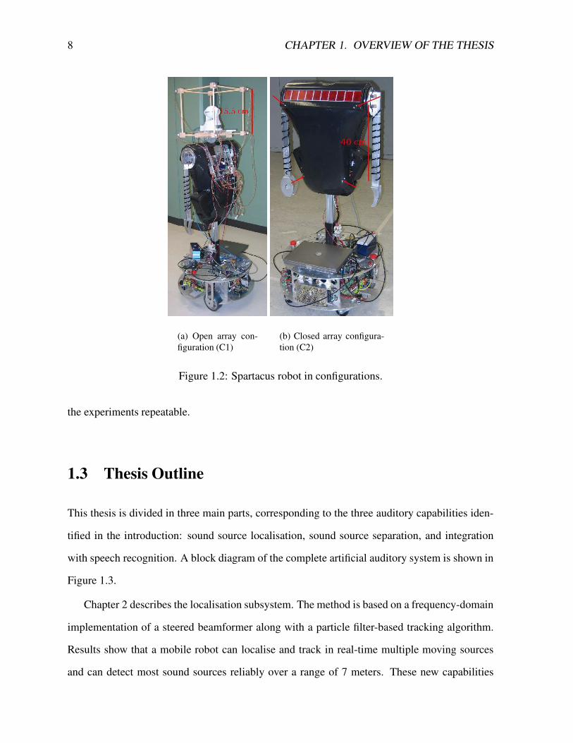
the Spartacus robot (shown in Figure 1.2a). The second configuration (C2) is a closed array and
uses smaller, middle-range (∼US$20 each) microphones, placed through holes (Figure 1.1b) at
different locations on the body of the robot (shown in Figure 1.2b). Although we are mainly
interested in the C2 configuration because it is the least intrusive, the C1 configuration is used
4http://www.inel.gov/featurestories/12-01robots.shtml

1.2. EXPERIMENTAL SETUP 7
to demonstrate the validity of some of the hypotheses we make, as well as the adaptability of
the system. It is reported that better localisation and separation results are obtained when max-
imising the distance between the microphones [30]. So, given the fact that we desire uniform
performance regardless of the location of the sources, we spread the microphones evenly (and
as far away from each other as possible) on the robot surface.
(a) Electret with pre-amplifier (C1)
(b) Electret installed directly onthe robot frame (C2)
Figure 1.1: Microphones used on the Spartacus robot.
For both arrays, all channels are sampled simultaneously using an RME Hammerfall Mul-
tiface DSP connected to a notebook computer (Pentium-M 1.6 GHz CPU) through a CardBus
interface. The software part is implemented within the FlowDesigner5 environment and is de-
signed to be connected to other components of the robot through the MARIE6 framework, as
described in [31].
Experiments are performed in two different environments. The first environment (E1) is a
medium-size room (10 m × 11 m, 2.5 m ceiling) with a reverberation time (-60 dB) of 350 ms
and moderate noise (ventilation, computers). The second environment (E2) is a hall (16 m ×
17 m, 3.1 m ceiling, connected to other rooms) with a reverberation time of approximately 1.0 s
and a high level of background noise. While E2 is a public area, we tried to minimise the noise
(by not having people close to the experimental setup) made by other people in order to make
5http://flowdesigner.sourceforge.net/6http://marie.sourceforge.net/
8 CHAPTER 1. OVERVIEW OF THE THESIS
(a) Open array con-figuration (C1)
(b) Closed array configura-tion (C2)
Figure 1.2: Spartacus robot in configurations.
the experiments repeatable.
1.3 Thesis Outline
This thesis is divided in three main parts, corresponding to the three auditory capabilities iden-
tified in the introduction: sound source localisation, sound source separation, and integration
with speech recognition. A block diagram of the complete artificial auditory system is shown in
Figure 1.3.
Chapter 2 describes the localisation subsystem. The method is based on a frequency-domain
implementation of a steered beamformer along with a particle filter-based tracking algorithm.
Results show that a mobile robot can localise and track in real-time multiple moving sources
and can detect most sound sources reliably over a range of 7 meters. These new capabilities

1.3. THESIS OUTLINE 9
Figure 1.3: Overview of the proposed artificial auditory system.
allow a mobile robot to interact with people in real life settings.
Chapter 3 presents a method for separating simultaneous sound sources for the separation
subsystem. The microphone array and the sound localisation data are used in a real-time im-
plementation of the Geometric Source Separation [32] algorithm. A multi-source post-filter is
also developed in order to further reduce interferences from other sources as well as background
noise. The main advantage of our approach for mobile robots resides in the fact that both the
frequency-domain Geometric Source Separation algorithm and the post-filter are able to adapt
rapidly to new sources and non-stationarity. Separation results are presented for three simulta-
neous interfering speakers in the presence of noise. A reduction of log spectral distortion (LSD)
and increase of signal-to-noise ratio (SNR) of approximately 8.9 dB and 13.7 dB are observed.
When the source of interest is silent, background noise and interference is reduced by 24.5 dB.
Chapter 4 demonstrates the use of the sound separation system to give a mobile robot the
ability to perform automatic speech recognition with simultaneous speakers. Two different
configurations for speech recognition are tested. In one configuration, the separated audio is
sent directly to an automatic speech recogniser (ASR). In the second configuration, the post-

10 CHAPTER 1. OVERVIEW OF THE THESIS
filter described in Chapter 3 is used to estimate the reliability of spectral features and compute
a missing feature mask that provides the ASR with information about the reliability of spectral
features. We show that it is possible to perform speech recognition for up to three simultaneous
speakers, even in a reverberant environment.
Chapter 5 concludes this thesis by summarising the results obtained, listing possible future
work, and suggesting applications of this work to other fields.
Chapter 2
Sound Source Localisation
Sound source localisation is defined as the determination of the coordinates of sound sources
in relation to a point in space. To perform sound localisation, our brain combines timing (more
specifically delay or phase) and amplitude information from the sound perceived by our two ears
[33], sometimes in addition to information from other senses. However, localising sound sources
using only two inputs is a challenging task. The human auditory system is very complex and
resolves the problem by accounting for the acoustic diffraction around the head and the ridges
of the outer ear. Without this ability, localisation with two microphones is limited to azimuth
only, along with the impossibility to distinguish if the sounds come from the front or the back.
Also, obtaining high-precision readings when the sound source is in the same axis as the pair of
microphones is more difficult.
One advantage with robots is that they do not have to inherit the same limitations as liv-
ing creatures. Using more than two microphones allows reliable and accurate localisation in
three dimensions (azimuth and elevation). Also, having multiple signals provides additional
redundancy, reducing the uncertainty caused by the noise and non-ideal conditions such as re-
verberation and imperfect microphones. It is with this principle in mind that we have developed
an approach allowing to localise sound sources using an array of microphones.
Our approach is based on a frequency-domain beamformer that is steered in all possible di-
11

12 CHAPTER 2. SOUND SOURCE LOCALISATION
rections to detect sources. Instead of measuring TDOAs and then converting to a position, the
localisation process is performed in a single step. This makes the system more robust, espe-
cially in the case where an obstacle prevents one or more microphones from properly receiving
the signals. The results of the localisation process are then enhanced by probability-based post-
processing, which prevents false detection of sources. This makes the system sensitive enough
for simultaneous localisation of multiple moving sound sources. This approach is an extension
of earlier work [34] and works for both far-field and near-field sound sources. Detection relia-
bility, accuracy, and tracking capabilities of the approach are validated using the Spartacus robot
platform, with different types of sound sources.
This chapter is organised as follows. Section 2.1 situates our work in relation to other
research projects in the field. Section 2.2 presents a brief overview of the system. Section 2.3
describes our steered beamformer implemented in the frequency-domain. Section 2.4 explains
how we enhance the results from the beamformer using a probabilistic post-processor. This is
followed by experimental results in Section 2.5, showing how the system behaves under different
conditions. Section 2.6 concludes the chapter and presents future work on sound localisation.
2.1 Related Work
Most of the work in relation to localisation of sound sources has been done using only two
microphones. This is the case with the SIG robot that uses both inter-aural phase difference
(IPD) and inter-aural intensity difference (IID) to locate sounds [12]. The binaural approach has
limitations when it comes to evaluating elevation and usually, the front-back ambiguity cannot
be resolved without resorting to active audition [35].
More recently, approaches using more than two microphones have been developed. One
approach uses a circular array of eight microphones to locate sound sources using the MUSIC
algorithm [22], a signal subspace approach. In our previous work also using eight microphones
[36], we presented a method for localising a single sound source where time delay of arrival

2.2. SYSTEM OVERVIEW 13
(TDOA) estimation was separated from the direction of arrival (DOA) estimation. It was found
that a system combining TDOA and DOA estimation in a single step improves the system’s
robustness, while allowing localisation (but not tracking) of simultaneous sources [34]. Kagami
et al. [37] reports a system using 128 microphones for 2D sound localisation of sound sources.
Similarly, Wang et al. [38] use 24 fixed microphones to track a moving robot in a room.
However, it would not be practical to include such a large number of microphones on a mobile
robot.
Most of the work so far on localisation of source sources does not address the problem of
tracking moving sources. It is proposed in [39] to use a Kalman filter for tracking a moving
source. However the proposed method assumes that a single source is present. In the past
years, particle filtering [40] (a sequential Monte Carlo method) has been increasingly popular to
resolve object tracking problems. Ward et al. [41, 42] and Vermaak [43] use this technique for
tracking single sound sources. Asoh et al. [23] even suggested to use this technique for mixing
audio and video data to track speakers. But again, the technique is limited to a single source
due to the problem of associating the localisation observation data to each of the sources being
tracked. We refer to that problem as the source-observation assignment problem. Some attempts
are made at defining multi-modal particle filters in [44], and the use of particle filtering for
tracking multiple targets is demonstrated in [45, 46, 47]. But so far, the technique has not been
applied to sound source tracking. Our work demonstrates that it is possible to track multiple
sound sources using particle filters by solving the source-observation assignment problem.
2.2 System Overview
The proposed localisation and tracking system, as shown in Figure 2.1, is composed of three
parts:
• A microphone array;
• A memoryless localisation algorithm based on a steered beamformer;

14 CHAPTER 2. SOUND SOURCE LOCALISATION
• A particle filtering tracker.
The array is composed of up to eight omni-directional microphones mounted on the robot. Since
the system is designed to be installed on any robot, there is no strict constraint on the position of
the microphones: only their positions must be known in relation to each other (measured with
∼0.5 cm accuracy). The microphone signals are used by a beamformer (spatial filter) that is
steered in all possible directions in order to maximise the output energy. The initial localisation
performed by the steered beamformer is then used as the input of a post-processing stage that
uses particle filtering to simultaneously track all sources and prevent false detections. The output
of the localisation system can be used to direct the robot attention to the source. It can also be
used as part of a source separation algorithm to isolate the sound coming from a single source,
as described in Chapter 3.
Steeredbeamformer
.
.
.
Particlefiltering
Sourceslocation
Omni-directionalmicrophones
Beamformerenergy
Figure 2.1: Overview of the Localisation subsystem.
2.3 Localisation Using a Steered Beamformer
The basic idea behind the steered beamformer approach to source localisation is to direct a
beamformer in all possible directions and look for maximal output. This can be done by max-
imising the output energy of a simple delay-and-sum beamformer. The formulation in both
time and frequency domain is presented in Section 2.3.1. Section 2.3.2 describes the frequency-

2.3. LOCALISATION USING A STEERED BEAMFORMER 15
domain weighting performed on the microphone signals and Section 2.3.3 shows how the search
is performed. A possible modification for improving the resolution is described in Section 2.3.4.
2.3.1 Delay-And-Sum Beamformer
The output y(nt)of an N -microphone delay-and-sum beamformer is defined as:
y(nt) =
N−1∑
n=0
xn (nt − τn) (2.1)
where xn (nt) is the signal from the nth microphone and τn is the delay of arrival for that
microphone. The output energy of the beamformer over a frame of length L is thus given
by:
E =L−1∑
nt=0
[y(nt)]2
=L−1∑
nt=0
[x0 (nt − τ0) + . . .+ xN−1 (nt − τN−1)]2 (2.2)
Assuming that only one sound source is present, we can see that E will be maximal when
the delays τn are such that the microphone signals are in phase, and therefore add constructively.
One problem with this technique is that energy peaks are very wide [48], which means that
the accuracy on τn is poor. Moreover, in the case where multiple sources are present, it is likely
for the two or more energy peaks to overlap, making them impossible to distinguish. One way
to narrow the peaks is to whiten the microphone signals prior to computing the energy [49].
Unfortunately, the coarse-fine search method as proposed in [48] cannot be used in that case
because the narrow peaks can then be missed during the coarse search. Therefore, a full fine
search is necessary, which requires increased computing power.
It is however possible to reduce the amount of computation by calculating the beamformer
energy in the frequency domain. This also has the advantage of making the whitening of the
signal easier. To do so, the beamformer output energy in Equation 2.2 can be expanded as:

16 CHAPTER 2. SOUND SOURCE LOCALISATION
E =
N−1∑
n=0
L−1∑
nt=0
x2n (nt − τn)
+ 2
N−1∑
n1=0
n1−1∑
n2=0
L−1∑
nt=0
xn1 (nt − τn1) xn2 (nt − τn2) (2.3)
which in turn can be rewritten in terms of cross-correlations:
E = K + 2
N−1∑
n1=0
n1−1∑
n2=0
Rxn1 ,xn2(τn1 − τn2) (2.4)
where K =∑N−1
n=0
∑L−1nt=0 x
2n (nt − τn) is nearly constant with respect to the τm delays and can
thus be ignored when maximisingE. The cross-correlation function can be approximated in the
frequency domain as:
Rij(τ) ≈L−1∑
k=0
Xi(k)Xj(k)∗e2πkτ/L (2.5)
where Xi(k) is the discrete Fourier transform of xi(nt), Xi(k)Xj(k)∗ is the cross-spectrum of
xi(nt) and xj(nt) and (·)∗ denotes the complex conjugate. The power spectra and cross-power
spectra are computed on overlapping windows (50% overlap) of L = 1024 samples at 48 kHz.
The cross-correlations Rij(τ) are computed by averaging the cross-power spectra Xi(k)Xj(k)∗
over a time period of 4 frames (40 ms). Once the Rij(τ) are pre-computed, it is possible to
computeE using onlyN(N−1)/2 lookup and accumulation operations, whereas a time-domain
computation would require 2L(N + 2) operations. For example, for N = 8 microphones and
Ng = 2562 directions, it follows that the complexity of the search itself is reduced from 1.2
Gflops to only 1.7 Mflops. After counting all time-frequency transformations, the complexity is
only 48.4 Mflops, 25 times less than a time domain search with the same resolution.

2.3. LOCALISATION USING A STEERED BEAMFORMER 17
2.3.2 Spectral Weighting
In the frequency domain, the whitened cross-correlation (also known as the phase transform, or
PHAT) is computed as:
R(w)ij (τ) ≈
L−1∑
k=0
Xi(k)Xj(k)∗
|Xi(k)| |Xj(k)|e2πkτ/L (2.6)
While it produces much sharper cross-correlation peaks, the whitened cross-correlation has
one drawback: each frequency bin of the spectrum contributes the same amount to the final
correlation, even if the signal at that frequency is dominated by noise. This makes the system
less robust to noise, while making detection of voice (which has a narrow bandwidth) more
difficult. In order to alleviate the problem, we introduce a weighting function that acts as a mask
based on the signal-to-noise ratio (SNR). For microphone i, we define this weighting function
as:
ζ`i (k) =ξ`i (k)
ξ`i (k) + 1(2.7)
where ξ`i (k) is an estimate of the a priori SNR at the ith microphone, at time frame `, for
frequency k. It is computed using the decision-directed approach proposed by Ephraim and
Malah [50]:
ξ`i (k) =(1− αd)
[
ζ`−1i (k)
]2 ∣∣X`−1
i (k)∣
∣
2+ αd
∣
∣X`i (k)
∣
∣
2
σ2i (k)
(2.8)
where αd = 0.1 is the adaptation rate and σ2i (k) is the noise estimate for microphone i. It
is easy to estimate σ2i (k) using the Minima-Controlled Recursive Average (MCRA) technique
[51], which adapts the noise estimate during periods of low energy.
It is also possible to make the system more robust to reverberation by modifying the weight-
ing function to include a reverberation term λrevi (k, `) to the noise estimate at time frame `. We
use a simple reverberation model with exponential decay:
λrevi (k, `) = γλrevi (k, `) +(1− γ)
δ
∣
∣ζ`i (k)X`−1i (k)
∣
∣
2(2.9)

18 CHAPTER 2. SOUND SOURCE LOCALISATION
where γ represents the reverberation time (T60) of the room (γ = 10−6/T60 ), δ is the Signal-
to-Reverberant Ratio (SRR) and λrevi (k,−1) = 0. In some sense, Equation 2.9 can be seen as
modelling the precedence effect [52, 53] in order to give less weight to frequency bins where a
loud sound was recently present. The resulting enhanced cross-correlation is defined as:
R(e)ij (τ) =
L−1∑
k=0
ζi(k)Xi(k)ζj(k)Xj(k)∗
|Xi(k)| |Xj(k)|e2πkτ/L (2.10)
The spectral weighting described above has similarities with the maximum likelihood (ML)
weighting described in [54], with two main differences. The first is that the weight we use
requires a lower complexity because it can be applied directly to the spectrum of the signals.
The second difference is that in high SNR conditions, the cross-correlation peak can take very
large values, and is thus be more difficult to use for evaluating the probability that a source is
really present (see Section 2.4.2).
The advantage of our approach over the simpler PHAT lies in the fact that the PHAT does
not take into account noise at all and assumes that the signal-to-reverberant ratio (SRR) is con-
stant across frequency [54]. The latter assumption only holds when the signal being tracked is
relatively stationary (i.e., no transients) compared to the reverberation time. For this reason, the
PHAT cannot model the precedence effect. In practice, it was found that when the presence of
a sound source is known, the localisation accuracy using our weighting similar to that obtained
using the PHAT. The main difference is that our weighting makes it easier to estimate if a source
is really present. As far as we are aware, no other work focuses on sound source localisation
when the number of sources present is unknown (and detection becomes important).
2.3.3 Direction Search on a Spherical Grid
In order to reduce the computation required and to make the system isotropic, we define a
uniform triangular grid for the surface of a sphere. To create the grid, we start with an initial
icosahedral grid [55]. Each triangle in the initial 20-element grid is recursively subdivided into

2.3. LOCALISATION USING A STEERED BEAMFORMER 19
four smaller triangles, as shown in Figure 2.2. The resulting grid is composed of 5120 triangles
and 2562 points. The beamformer energy is then computed for the hexagonal region associated
with each of these points. Each of the 2562 regions covers a radius of about 2.5◦ around its
centre, setting the resolution of the search.
(a) Icosahedral grid (b) Subdivison by four (onelevel)
(c) Subdivison by sixteen (twolevels)
Figure 2.2: Recursive subdivision of a triangular element.
Algorithm 1 Steered beamformer direction search.for all grid index k doEk ← 0for all microphone pair ij doτ ← lookup(k, ij)
Ek ← Ek +R(e)ij (τ)
end forend fordirection of source← argmaxk (Ek)
Once the cross-correlations R(e)ij (τ) are computed, the search for the best direction on the
grid is performed as described by Algorithm 1. The lookup parameter is a pre-computed table
of the time delay of arrival (TDOA) for each microphone pair and each direction on the sphere.
Using the far-field assumption as illustrated in Figure 2.3, the TDOA in samples is computed

20 CHAPTER 2. SOUND SOURCE LOCALISATION
using the cosine law [36]:
cosφ =cτij/Fs‖~pi − ~pj‖
=(~pi − ~pj) · ~u‖~pi − ~pj‖ ‖~u‖
(2.11)
where ~pi is the position of microphone i, ~u is a unit-vector that points in the direction of the
source, c is the speed of sound and Fs is the sampling rate. Isolating τij from Equation 2.11 and
knowing that ~u is a unit vector, we obtain:
τij =Fsc
(~pi − ~pj) · ~u (2.12)
pi
u
θφ
sourc
e dire
ction
microphone imicrophone j
cτij / Fs
pj
Figure 2.3: TDOA for the far field approximation.
Equation 2.12 assumes that the time delay is proportional to the distance between the source
and microphone. This is only true when there is no diffraction involved. While this hypothesis is
only verified for an “open” array (all microphones are in line of sight with the source), in practice
we demonstrate experimentally (see Section 2.5) that the approximation is good enough for our
system to work for a “closed” array (in which there are obstacles within the array).
For an array of N microphones and an Ng-element grid, the algorithm requires N(N−1)Ng
table memory accesses and N(N − 1)Ng/2 additions. In the proposed configuration (Ng =
2562, N = 8), the accessed data can be made to fit entirely in a modern processor’s L2 cache.
Using Algorithm 1, our system is able to find the loudest source present by maximising the
energy of a steered beamformer. In order to localise other sources that may be present, the pro-

2.3. LOCALISATION USING A STEERED BEAMFORMER 21
Algorithm 2 Localisation of multiple sources.for q = 0 to Q− 1 doDq ← Steered beamformer direction searchfor all microphone pair ij doτ ← lookup(Dq, ij)
R(e)ij (τ) = 0
end forend for
cess is repeated by removing the contribution of the first source to the cross-correlations, leading
to Algorithm 2. Since we do not know how many sources are present, the number of sources
to find is set to the constant Q. Therefore, Algorithm 2 finds the Q loudest sources around the
array. We determined empirically that the maximum number of sources our beamformer is able
to locate at once is four. The fact that Algorithm 2 always finds four sources regardless of the
number of sources present leads to a high rate of false detection, even when four or more sources
are present. That problem is handled by the particle filter described in Section 2.4.
2.3.4 Direction Refining
When a source is located using Algorithm 1, the direction accuracy is limited by the size of
the grid used. It is however possible, as an optional step, to further refine the source location
estimate. In order to do so, we define a refined grid for the surrounding of the point where
a source was found. To take into account the near-field effects, the grid is refined in three
dimensions: horizontally, vertically and over distance. Using five points in each direction, we
obtain a 125-point local grid with a maximum error of around 1◦. For the near-field case,
Equation 2.12 no longer holds, so it is necessary to compute the time differences as:
τij =Fsc
(‖d~u− ~pj‖ − ‖d~u− ~pi‖) (2.13)
where d is the distance between the source and the centre of the array. Equation 2.13 is evaluated
for five distances d (ranging from 50 cm to 5 m) in order to find the direction of the source with

22 CHAPTER 2. SOUND SOURCE LOCALISATION
improved accuracy. Unfortunately, it was observed that the value of d found in the search is
too unreliable to provide a good estimate of the distance between the source and the array. The
incorporation of the distance nonetheless allows improved accuracy for the near field case.
2.4 Particle-Based Tracking
The steered beamformer detailed in Section 2.3 provides only instantaneous, noisy information
about sources being possibly present, and no information about the behaviour of the source in
time (i.e. tracking). For that reason, it is desirable to use a probabilistic temporal integration to
track the different sound sources based on all measurements available up to the current time.
It has been shown [41, 42, 23] that particle filters are an effective way of tracking sound
sources. The choice of particle filtering is further motivated by the fact that earlier work using
a fixed grid for tracking showed that the technique can not provide continuous tracking when
moving sources had short periods of silence. This can be observed in Figure 2.4, taken from
[34]. Particle filtering is also preferred to Kalman filtering because key aspects of the proposed
algorithm, such as the handling of false detections and source-observation assignment (see
Section 2.4.3), cannot be adequately modelled as a Gaussian process, as is assumed by the
Kalman filter [39].
Let S(t)j be the state variable associated to source j (j = 0, 1, . . . ,M −1) at time t, a particle
filter approximates the probability density function (pdf) of S(t)j as:
p(
S(t)j
)
≈Np∑
i=1
w(t)j,i δ(
S(t)j − s
(t)j,i
)
where δ(
S(t)j − s
(t)j,i
)
is the Dirac function for a particle of state s(t)j,i , w
(t)j,i is the particle weight
and Np is the number of particles. With this approach, each particle can be viewed as represent-
ing a hypothesis about the location of a sound source and the weights assigned to the particles
represent the probability for each hypothesis to be correct. The state vector for the particles is

2.4. PARTICLE-BASED TRACKING 23
0 5 10 15 20 25 30
−150
−100
−50
0
50
100
150
Time [s]
Ang
le [d
eg]
Speaker 1
Speaker 2
Speaker 3
Speaker 4
Speaker 1
Figure 2.4: Probabilistic tracking of multiple sources using a fixed grid.
composed of six dimensions, three for the position x(t)j,i and three for its derivative:
s(t)j,i =
x(t)j,i
x(t)j,i
(2.14)
Figure 2.5 illustrates the particle representation of two sources. The source in red is located
around 60 degrees azimuth and 15 degrees elevation while the source in green is located around
-60 degrees azimuth and 20 degrees elevation. The spread of the particles is an indicator of the
uncertainty on the source position.
Since the particle position is constrained to lie on a unit sphere and the speed is tangent to
the sphere, there are only four degrees of freedom. The particle filtering algorithm is outlined in
Algorithm 3 and generalises sound source tracking to an arbitrary and non-constant number of
sources. The steps are detailed in Subsections 2.4.1 to 2.4.7. The particle weights are updated by
taking into account observations obtained from the steered beamformer and by computing the
assignment between these observations and the sources being tracked. From there, the estimated
location of the source is the weighted mean of the particle positions.

24 CHAPTER 2. SOUND SOURCE LOCALISATION
-10
0
10
20
30
40
-100 -50 0 50 100
Ele
vatio
n [d
eg]
Azimuth [deg]
-10
0
10
20
30
40
-100 -50 0 50 100
Ele
vatio
n [d
eg]
Azimuth [deg]
Figure 2.5: Example of two sources being represented by a particle filter.
Algorithm 3 Particle-based tracking algorithm. Steps 1 to 7 correspond to Subsections 2.4.1 to2.4.7.
1. Predict the state s(t)j from s
(t−1)j for each source j.
2. Compute instantaneous direction probabilities associated with the steered beamformerresponse.
3. Compute probabilities P (t)q,j associating beamformer peaks to sources being tracked.
4. Compute updated particle weights w(t)j,i .
5. Add or remove sources if necessary.
6. Compute source localisation estimate x(t)j for each source.
7. Resample particles for each source if necessary and go back to step 1.
2.4.1 Prediction
The prediction step in particle filtering plays a similar role as for the Kalman filter. However,
instead of explicitly predicting the mean and variance of the model, the particles are subjected
to a stochastic excitation with damping model as proposed in [42]:

2.4. PARTICLE-BASED TRACKING 25
x(t)j,i = ax
(t−1)j,i + bFx (2.15)
x(t)j,i = x
(t−1)j,i + ∆T x
(t)j,i (2.16)
where a = e−α∆T controls the damping term, b = β√
1− a2 controls the excitation term, Fx
is a normally distributed random variable of unit variance and ∆T is the time interval between
updates. In addition, we consider three possible states:
• Stationary source (α = 2, β = 0.04);
• Constant velocity source (α = 0.05, β = 0.2);
• Accelerated source (α = 0.5, β = 0.2).
A normalisation step1 ensures that x(t)i still lies on the unit sphere (
∥
∥
∥x
(t)j,i
∥
∥
∥= 1) after applying
Equations 2.15 and 2.16.
2.4.2 Instantaneous Direction Probabilities from Beamformer Response
The steered beamformer described in Section 2.3 produces an observation O(t) for each time t.
The observation O(t) =[
O(t)0 . . . O
(t)Q−1
]
is composed of Q potential source locations yq found
by Algorithm 2. We also denote O(t), the set of all observations O(t) up to time t. We introduce
the probability Pq that the potential source q is a true source (not a false detection). The value
of Pq can be interpreted as our confidence in the steered beamformer output. For the first source
(q = 0), we have observed that the higher the beamformer energy, the more likely that potential
source is to be true. However, for the other potential sources (q > 0), false alarms are very
frequent and independent of energy. With this in mind, for the four potential sources q, we
1The normalisation is performed as x(t)i ← x
(t)i /
∥
∥
∥x(t)i
∥
∥
∥.

26 CHAPTER 2. SOUND SOURCE LOCALISATION
define Pq empirically as:
Pq =
ν2/2, q = 0, ν ≤ 1
1− ν−2/2, q = 0, ν > 1
0.3, q = 1
0.16, q = 2
0.03, q = 3
(2.17)
with ν = E0/ET , where ET is a threshold that depends on the number of microphones, the
frame size and the analysis window used (we empirically found that ET = 150 is appropriate
for eight microphones). Figure 2.6 shows an example of Pq values for potential sources found
by the steered beamformer in a case with four moving sources2. It is possible to distinguish four
trajectories, but it can be seen that the observations from the steered beamformer are nonetheless
very noisy.
-150
-100
-50
0
50
100
150
0 5 10 15 20 25 30 35
Azi
mut
h [d
eg]
Time [s]
Figure 2.6: Beamformer output probabilities Pq for azimuth as a function of time. Observationswith Pq > 0.5 shown in red, 0.2 < Pq < 0.5 in blue, Pq < 0.2 in green.
At time t, the probability density of observing O(t)q for a source located at particle position
x(t)j,i is given by:
p(
O(t)q
∣
∣x(t)j,i
)
= N(
yq;xj,i; σ2)
(2.18)
2Only the azimuth part of yq is shown as a function of time.

2.4. PARTICLE-BASED TRACKING 27
where N (yq;xj,i; σ2) is a normal distribution centred at xj,i with variance σ2 evaluated at yq,
and models the localisation accuracy of the steered beamformer. We use σ = 0.05, which
corresponds to an RMS error of 3 degrees for the location found by the steered beamformer.
2.4.3 Probabilities for Multiple Sources
Before we can derive the update rule for the particle weights w(t)j,i , we must first introduce the
concept of source-observation assignment. For each potential source q detected by the steered
beamformer, there are three possibilities:
• It is a false detection (H0).
• It corresponds to one of the sources currently tracked (H1).
• It corresponds to a new source that is not yet being tracked (H2).
In the case of H1, we need to determine which tracked source j corresponds to potential source
q. First, we assume that a potential source may correspond to at most one tracked source and
that a tracked source can correspond to at most one potential source.
New source
Falsedetection
Potentialsource q
Trackedsource j
Not observed
Figure 2.7: Assignment example where two of the tracked sources are observed, with onenew source and one false detection. The assignment can be described as f({0, 1, 2, 3}) ={1,−2, 0,−1}.
Let f : {0, 1, . . . , Q−1} −→ {−2,−1, 0, 1, . . . ,M−1} be a function assigning observation
q to the source j (values -2 is used for false detection and -1 is used for a new source). Figure 2.7
28 CHAPTER 2. SOUND SOURCE LOCALISATION
illustrates a hypothetical case with four potential sources detected by the steered beamformer
and their assignment to the tracked sources. Knowing P(
f∣
∣O(t))
(the probability that f is the
correct assignment given observation O(t)) for all possible f , we can derive Pq,j, the probability
that the tracked source j corresponds to the potential source q as:
P(t)q,j =
∑
f
δj,f(q)P(
f∣
∣O(t))
(2.19)
P (t)q (H0) =
∑
f
δ−2,f(q)P(
f∣
∣O(t))
(2.20)
P (t)q (H2) =
∑
f
δ−1,f(q)P(
f∣
∣O(t))
(2.21)
where δi,j is the Kronecker delta. Equation 2.19 is in fact the sum of the probabilities of all f
that assign potential source q to tracked source j and similarly for Equations 2.20 and 2.21.
Omitting t for clarity, the probability P (f |O) is given by:
P (f |O) =p(O|f)P (f)
p(O)(2.22)
Knowing that there is only one correct assignment (∑
f P (f |O) = 1), we can avoid computing
the denominator p(O) by using normalisation. Assuming conditional independence of the ob-
servations given the mapping function, we can decompose p (O| f) into individual components:
p (O| f) =∏
q
p (Oq| f(q)) (2.23)
We assume that the distribution of the false detections (H0) and the new sources (H2) are
uniform, while the distribution for tracked sources (H1) is the pdf approximated by the particle
distribution convolved with the steered beamformer error pdf:
p (Oq| f(q)) =
1/4π, f(q) = −2
1/4π, f(q) = −1∑
i wf(q),ip (Oq|xj,i) , f(q) ≥ 0
(2.24)

2.4. PARTICLE-BASED TRACKING 29
The a priori probability of f being the correct assignment is also assumed to come from inde-
pendent individual components, so that:
P (f) =∏
q
P (f(q)) (2.25)
with:
P (f(q)) =
(1− Pq)Pfalse, f(q) = −2
PqPnew f(q) = −1
PqP(
Obs(t)j
∣
∣O(t−1))
f(q) ≥ 0
(2.26)
where Pnew is the a priori probability that a new source appears and Pfalse is the a priori
probability of false detection. The probability P(
Obs(t)j
∣
∣O(t−1))
that source j is observable
(i.e., that it exists and is active) at time t is given by:
P(
Obs(t)j
∣
∣O(t−1))
= P(
Ej∣
∣O(t−1))
P(
A(t)j
∣
∣O(t−1))
(2.27)
where Ej is the event that source j actually exists and A(t)j is the event that it is active (but
not necessarily detected) at time t. By active, we mean that the signal it emits is non-zero (for
example, a speaker who is not making a pause). The probability that the source exists is given
by:
P(
Ej∣
∣O(t−1))
= P(t−1)j +
(
1− P (t−1)j
) PoP(
Ej∣
∣O(t−2))
1− (1− Po)P (Ej |O(t−2) )(2.28)
where Po is the a priori probability that a source is not observed (i.e., undetected by the steered
beamformer) even if it exists (with P0 = 0.2 in our case) and P (t)j =
∑
q P(t)q,j is the probability
that source j is observed (assigned to any of the potential sources).
Assuming a first order Markov process, we can write the following about the probability of
source activity:
P(
A(t)j
∣
∣O(t−1))
= P(
A(t)j
∣
∣
∣A
(t−1)j
)
P(
A(t−1)j
∣
∣O(t−1))
+P(
A(t)j
∣
∣
∣¬A
(t−1)j
) [
1− P(
A(t−1)j
∣
∣O(t−1))]
(2.29)

30 CHAPTER 2. SOUND SOURCE LOCALISATION
with P(
A(t)j
∣
∣
∣A
(t−1)j
)
the probability that an active source remains active (set to 0.95), and
P(
A(t)j
∣
∣
∣¬A
(t−1)j
)
the probability that an inactive source becomes active again (set to 0.05).
Assuming that the active and inactive states are equiprobable, the activity probability is com-
puted using Bayes’ rule and usual probability manipulations:
P(
A(t)j
∣
∣O(t))
=1
1 +
h
1−P“
A(t)j |O(t−1)
”ih
1−P“
A(t)j |O(t)
”i
P“
A(t)j |O(t−1)
”
P“
A(t)j |O(t)
”
(2.30)
2.4.4 Weight Update
At times t, the new particle weights for source j are defined as:
w(t)j,i = p
(
x(t)j,i
∣
∣O(t))
(2.31)
Assuming that the observations are conditionally independent given the source position, and
knowing that for a given source j,∑Np
i=1 w(t)j,i = 1, we obtain through Bayesian inference:
w(t)j,i =
p(
O(t)∣
∣x(t)j,i
)
p(
x(t)j,i
)
p (O(t))
=p(
O(t)∣
∣x(t)j,i
)
p(
O(t−1)∣
∣x(t)j,i
)
p(
x(t)j,i
)
p (O(t))
=p(
xj,i∣
∣O(t))
p(
x(t)j,i
∣
∣O(t−1))
p(
O(t))
p(
O(t−1))
p (O(t)) p(
x(t)j,i
)
=p(
x(t)j,i
∣
∣O(t))
w(t−1)j,i
∑Npi=1 p
(
x(t)j,i |O(t)
)
w(t−1)j,i
(2.32)
Let I (t)j denote the event that source j is observed at time t and knowing that P
(
I(t)j
)
=
P(t)j =
∑
q P(t)q,j , we have:

2.4. PARTICLE-BASED TRACKING 31
p(
x(t)j,i
∣
∣O(t))
=(
1− P (t)j
)
p(
x(t)j,i
∣
∣
∣O(t),¬I (t)
j
)
+ P(t)j p
(
x(t)j,i
∣
∣
∣O(t), I
(t)j
)
(2.33)
In the case where no observation matches the source, all particles have the same probability, so
we obtain:
p(
x(t)j,i
∣
∣O(t))
=(
1− P (t)j
) 1
Np
+ Pj
∑Qq=1 P
(t)q,j p
(
O(t)q
∣
∣
∣x
(t)j,i
)
∑Ni=1
∑Qq=1 P
(t)q,j p
(
O(t)q
∣
∣
∣x
(t)j,i
) (2.34)
where the denominator on the right side of Equation 2.34 provides normalisation for the I (t)j
case, so that∑N
i=1 p(
x(t)j,i
∣
∣
∣O(t), I
(t)j
)
= 1.
2.4.5 Adding or Removing Sources
In a real environment, sources may appear or disappear at any moment. If, at any time, Pq(H2)
is higher than a threshold empirically set3 to 0.3, we consider that a new source is present. In
that case, a set of particles is created for source q. Even when a new source is created, it is only
assumed to exist if its probability of existence P(
Ej∣
∣O(t))
reaches a certain threshold, which
we empirically set4 to 0.98. At this point, the probability of existence is set to 1 and ceases to
be updated.
In the same way, we set a time limit (typically two seconds) on sources. If the source has
not been observed (P (t)j < Tobs) for a certain amount of time, we consider that it no longer
exists. In that case, the corresponding particle filter is no longer updated nor considered in
future calculations. The value of Tobs only determines whether a discontinuous source will be
considered as one or two sources.
3The value must be small enough for all sources to be detected, but large enough to prevent a large number offalse alarms from being tracked.
4The exact value does not have a significant impact on the performance of the system

32 CHAPTER 2. SOUND SOURCE LOCALISATION
2.4.6 Parameter Estimation
The estimated position x(t)j of each source is the mean of the pdf and can be obtained as a
weighted average of its particles position:
x(t)j =
Np∑
i=1
w(t)j,ix
(t)j,i (2.35)
It is however possible to obtain better accuracy simply by adding a delay to the algorithm.
This can be achieved by augmenting the state vector by past position values. At time t, the
position at time t− T is thus expressed as:
x(t−T )j =
Np∑
i=1
w(t)j,ix
(t−T )j,i (2.36)
Using the same example as in Figure 2.6, Figure 2.8 represents how the particle filter is able to
remove the noise and produce smooth trajectories. The added delay produces an even smoother
result.
-150
-100
-50
0
50
100
150
0 5 10 15 20 25 30 35
Azi
mut
h [d
eg]
Time [s]
(a) No delay
-150
-100
-50
0
50
100
150
0 5 10 15 20 25 30 35
Azi
mut
h [d
eg]
Time [s]
(b) Delayed estimation (T=500 ms)
Figure 2.8: Tracking of four moving sources, showing azimuth as a function of time.

2.5. RESULTS 33
2.4.7 Resampling
Resampling is necessary in order to prevent the filter from degenerating to a single particle
of weight 1. During the resampling stage Np “new” particles are drawn from the original
Np particles with the probably of a particle being selected being proportional to its weight
w(t)j,i . After resampling, all particle weights are reset to 1/Np, preserving the original pdf. The
resampling step in particle filtering can be views as survival of the fittest, where the particles
with a large weight are more likely to be selected (and can be selected multiple times) than the
particles with a small weight.
Also, resampling is performed only whenNeff ≈(
∑Ni=1 w
2j,i
)−1
< Nmin [56] withNmin =
0.7N . That criterion ensures that resampling only occurs when new data is available for a certain
source. Otherwise, this would cause unnecessary reduction in particle diversity, due to some
particles randomly disappearing.
2.5 Results
Results for the localisation are obtained using the robot described in Section 1.2 with the C1 and
C2 configurations in the E1 and E2 environments. Running the localisation system in real-time
currently requires 30% of a 1.6 GHz Pentium-M CPU. Due to the low complexity of the particle
filtering algorithm, we are able to use 1000 particles per source without noticeable increase in
complexity. This also means that the CPU time does not increase significantly with the number
of sources present. For all tasks, configurations and environments, all parameters have the same
value, except for the reverberation decay γ, which is set to 0.65 (T60 = 350 ms) in the E1
environment and 0.85 (T60 = 910 ms) in the E2 environment. In both cases, the Signal-to-
Reverberant Ratio (SRR) δ is set to 3.3 (5.2 dB).

34 CHAPTER 2. SOUND SOURCE LOCALISATION
2.5.1 Characterisation
The system is characterised in environment E1 in terms of detection reliability and accuracy.
Detection reliability is defined as the capacity to detect and localise sounds to within 10 degrees,
while accuracy is defined as the localisation error for sources that are detected. We use three
different types of sound: a hand clap, the test sentence (“Spartacus, come here”), and a burst of
white noise lasting 100 ms. The sounds are played from a speaker placed at different locations
around the robot and at three different heights: 0.1 m, 1 m, 1.4 m.
2.5.1.1 Detection Reliability
Detection reliability is tested at distances (measured from the centre of the array) ranging from
1m (a normal distance for close interaction) to 7m (limitations of of the room). Three indicators
are computed: correct localisation (within 10 degrees), reflections (incorrect elevation due to
floor and ceiling), and other errors (repeated detection or large error). For all indicators, we
compute the number of occurrences divided by the number of sounds played. This test includes
1440 sounds at a 22.5◦ interval for 1 m and 3 m, and 360 sounds at a 90◦ interval for 5 m and 7
m).
Results are shown in Table 2.1 for both C1 and C2 configurations5. In configuration C1,
results show near-perfect reliability even at seven meter distance. For C2, we noted that the
reliability depends on the sound type, so detailed results for different sounds are provided in
Table 2.2, showing that only hand clap sounds cannot be reliably detected passed one meter. We
expect that a human would have achieved a score of 100% for this reliability test.
Like most localisation algorithms, our system is unable to detect pure tones. This behaviour
is explained by the fact that sinusoids occupy only a very small region of the spectrum and thus
have a very small contribution to the cross-correlations with the proposed weighting. It must be
noted that tones tend to be more difficult to localise than wideband signals even for the human
5The total for a configuration does not have to be equal to 100% percent because there are cases where nothingis detected and other cases where an error occurs in addition to correct localisation.

2.5. RESULTS 35
auditory system6.
Table 2.1: Detection reliability for C1 and C2 configurations.
Distance Correct (%) Reflection (%) Other error (%)C1 C2 C1 C2 C1 C2
1 m 100 94.2 0.0 7.3 0.0 1.33 m 99.4 80.6 0.0 21.0 0.3 0.15 m 98.3 89.4 0.0 0.0 0.0 1.17 m 100 85.0 0.6 1.1 0.6 1.1
Table 2.2: Correct localisation rate as a function of sound type and distance for C2 configuration.
Distance Hand clap (%) Speech (%) Noise burst (%)1 m 88.3 98.3 95.83 m 50.8 97.9 92.95 m 71.7 98.3 98.37 m 61.7 95.0 98.3
2.5.1.2 Localisation Accuracy
In order to measure the accuracy of the localisation system, we use the same setup as for
measuring reliability, with the exception that only distances of 1 m and 3 m are tested (1440
sounds at a 22.5◦ interval) due to limited space available in the testing environment. Neither
distance nor sound type has significant impact on accuracy. The root mean square accuracy
results are shown in Table 2.3 for configurations C1 and C2. Both azimuth and elevation are
shown separately. According to [57, 58], human sound localisation accuracy ranges between
two and four degrees in similar conditions. The localisation accuracy of our system is thus
equivalent or better than human localisation accuracy.
6Observed from personal experience.

36 CHAPTER 2. SOUND SOURCE LOCALISATION
Table 2.3: Localisation accuracy (root mean square error).
Localisation error C1 (deg) C2 (deg)Azimuth 1.10 1.44Elevation 0.89 1.41
2.5.2 Source Tracking
We measure the tracking capabilities of the system for multiple sound sources. These are
performed using the C2 configuration in both E1 and E2 environments. In all cases, the distance
between the robot and the sources is approximately two meters. The azimuth is shown as a
function of time for each source. The elevation is not shown as it is almost the same for all
sources during these tests. The trajectories of the sources in the three experiments are shown in
Figure 2.9. For each of the three cases, only one experiment was performed so that no selection
would have to be made about which trial to display.
(a) Moving sources (b) Moving robot (c) Sources with inter-secting trajectories
Figure 2.9: Source trajectories (robot represented as an X, sources represented with dots).
2.5.2.1 Moving Sources
In a first set of trials, four people were told to talk continuously (reading a text with normal
pauses between words) to the robot while moving, as shown on Figure 2.9a. Each person walked
90 degrees towards the left of the robot before walking 180 degrees towards the right.

2.5. RESULTS 37
Results are presented in Figure 2.10 for delayed estimation (T=500 ms). In both environ-
ments, the source estimated trajectories are consistent with the trajectories of the four speakers
and only one false detection was present for a short period of time.
-150
-100
-50
0
50
100
150
0 5 10 15 20 25 30 35
Azi
mut
h [d
eg]
Time [s]
(a) E1
-150
-100
-50
0
50
100
150
5 10 15 20 25 30 35 40
Azi
mut
h [d
eg]
Time [s]
(b) E2
Figure 2.10: Four speakers moving around a stationary robot. False detection shown in black(around t = 15 s in E1).
2.5.2.2 Moving Robot
Tracking capabilities of our system are also evaluated in the context where the the robot is
moving, as shown on Figure 2.9b. In this experiment, two people are talking continuously to
the robot as it is passing between them. The robot then makes a half-turn to the left. Results
are presented in Figure 2.11 for delayed estimation (T=500 ms). Once again, the estimated
source trajectories are consistent with the trajectories of the sources relative to the robot for
both environments. Only one false detection was present for a short period of time.
2.5.2.3 Sources with Intersecting Trajectories
In this experiment, two moving speakers are talking continuously to the robot, as shown on
Figure 2.9c. They start from each side of the robot, intersecting in front of the robot before
reaching the other side. Results for delayed estimation (T=500 ms) are presented in Figure 2.12

38 CHAPTER 2. SOUND SOURCE LOCALISATION
-150
-100
-50
0
50
100
150
5 10 15 20 25 30 35 40
Azi
mut
h [d
eg]
Time [s]
(a) E1
-150
-100
-50
0
50
100
150
5 10 15 20 25 30
Azi
mut
h [d
eg]
Time [s]
(b) E2
Figure 2.11: Four speakers moving around a stationary robot.Two stationary speakers with therobot moving. False detection shown in black (around t = 38 s in E1 and around t = 20 s inE2).
and show that the particle filter is able to keep track of each source. This result is possible
because the prediction step (Section 2.4.1) imposes some inertia to the sources.
-100
-50
0
50
100
2 4 6 8 10 12 14 16 18
Azi
mut
h [d
eg]
Time [s]
(a) E1
-100
-50
0
50
100
4 6 8 10 12 14 16
Azi
mut
h [d
eg]
Time [s]
(b) E2
Figure 2.12: Two speakers intersecting in front of the robot.
2.5.2.4 Number of Microphones
These results evaluate how the number of microphones used affect the system capabilities. To
do so, we use the same recording as in 2.5.2.1 for C2 in E1 with only a subset of the microphone
signals to perform localisation. Since a minimum of four microphones are necessary for localis-

2.5. RESULTS 39
ing sounds without ambiguity7, we evaluate the system for four to seven microphones (selected
arbitrarily as microphones number 1 through N ). Comparing results of Figure 2.13 to those
obtained in Figure 2.10 for E1, it can be observed that tracking capabilities degrade gracefully
as microphones are removed. While using seven microphones makes little difference compared
to the baseline of eight microphones, the system is unable to reliably track more than two of the
sources when only four microphones are used. Although there is no theoretical relationship be-
tween the number of microphones and the maximum number of sources that can be tracked, this
clearly shows how the redundancy added by using more microphones can help in the context of
sound source localisation.
-150
-100
-50
0
50
100
150
0 500 1000 1500 2000 2500 3000 3500 4000
Azi
mut
h [d
eg]
Time [s]
-150
-100
-50
0
50
100
150
0 500 1000 1500 2000 2500 3000 3500 4000
Azi
mut
h [d
eg]
Time [s]
-150
-100
-50
0
50
100
150
0 500 1000 1500 2000 2500 3000 3500 4000
Azi
mut
h [d
eg]
Time [s]
-150
-100
-50
0
50
100
150
0 500 1000 1500 2000 2500 3000 3500 4000
Azi
mut
h [d
eg]
Time [s]
4 microphones 5 microphones
6 microphones 7 microphones
Figure 2.13: Tracking of four sources using C2 in the E1 environment, using 4 to 7 microphones(ET adjusted to be proportional to the number of microphone pairs, T = 500 ms).
7With three microphones, it is not possible to distinguish sources on either side of the plane formed by themicrophones.

40 CHAPTER 2. SOUND SOURCE LOCALISATION
2.5.2.5 Audio Bandwidth
We evaluate the impact of audio bandwidth on the tracking capabilities using the same recording
as in 2.5.2.1 for C2 in E1. The input signal is low-pass filtered at different frequencies, while the
rest of the processing is still performed at 48 kHz, so that the cross-correlations are computed
at higher resolution. Figure 2.14 presents tracking results corresponding to 8 kHz sampling rate
and 16 kHz sampling rate, since those sampling rate have been used in other work [22, 39, 41,
54]. It can be observed that results are significantly degraded when compared to Figure 2.10,
especially in the case of 8 kHz sampling, where only two of the four sources could be tracked.
This can be explained by the fact that the spectrum of speech extends beyond 8 kHz and that
those higher frequencies can still contribute to the localisation process. Figure 2.14 justifies our
use of the full 20 kHz audio bandwidth.
-200
-150
-100
-50
0
50
100
150
200
0 500 1000 1500 2000 2500 3000 3500
Azi
mut
h [d
eg]
Time [s]
(a) 8 kHz sampling rate
-200
-150
-100
-50
0
50
100
150
200
0 500 1000 1500 2000 2500 3000 3500
Azi
mut
h [d
eg]
Time [s]
-200
-150
-100
-50
0
50
100
150
200
0 500 1000 1500 2000 2500 3000 3500
Azi
mut
h [d
eg]
Time [s]
-200
-150
-100
-50
0
50
100
150
200
0 500 1000 1500 2000 2500 3000 3500
Azi
mut
h [d
eg]
Time [s]
-200
-150
-100
-50
0
50
100
150
200
0 500 1000 1500 2000 2500 3000 3500
Azi
mut
h [d
eg]
Time [s]
-200
-150
-100
-50
0
50
100
150
200
0 500 1000 1500 2000 2500 3000 3500
Azi
mut
h [d
eg]
Time [s]
-200
-150
-100
-50
0
50
100
150
200
0 500 1000 1500 2000 2500 3000 3500
Azi
mut
h [d
eg]
Time [s]
(b) 16 kHz sampling rate
Figure 2.14: Tracking of four sources using C2 in the E1 environment for reduced audio band-width.
2.5.3 Localisation and Tracking for Robot Control
This experiment is performed in real-time and consists of making the robot follow the person
speaking to it. At any time, only the source present for the longest time is considered. When
the source is detected in front (within 10 degrees) of the robot, it is made to go forward. At the

2.6. DISCUSSION 41
same time, regardless of the angle, the robot turns toward the source in such a way as to keep
the source in front. Using this simple control system, it is possible to control the robot simply
by talking to it, even in noisy and reverberant environments.
This has been tested by controlling the robot going from environment E1 to environment E2,
having to go through corridors and an elevator, speaking to the robot with normal intensity at a
distance ranging from one meter to three meters. The system worked in real-time8, providing
tracking data at a rate of 25 Hz with no additional delay (T=0) on the estimator. The robot reac-
tion time is limited mainly by the inertia of the robot. One problem we encountered during the
experiment is that when going through corridors, the robot would sometimes detect reflections
on the walls in addition to the real sources. Fortunately, the fact that the robot considers only
the oldest source present reduces problems from both reflections and noise sources.
2.6 Discussion
Using an array of eight microphones, we have implemented a system that is able to localise and
track simultaneous moving sound sources in the presence of noise and reverberation, at distances
up to seven meters. We have also demonstrated that the system can successfully control the
motion of a robot in real-time, using only the direction of sounds. The tracking capabilities
demonstrated result from combining our frequency-domain steered beamformer with a particle
filter tracking multiple sources. Moreover, the solution we found to the source-observation
assignment problem is also applicable to other multiple objects tracking problems, like visual
tracking.
A robot using the proposed system has access to a rich, robust and useful set of informa-
tion derived from its acoustic environment. This can certainly affect its ability of making au-
tonomous decisions in real life settings, and show higher intelligent behaviour. Also, because
the system is able to localise multiple sound sources, it can be exploited by a sound separation
8A video of the experiment can be downloaded from http://www.gel.usherb.ca/laborius/projects/Audible/JMLocalization.mov

42 CHAPTER 2. SOUND SOURCE LOCALISATION
algorithm and enable speech recognition to be performed. This allows to identify the sound
sources so that additional relevant information can be obtained from the acoustic environment.
The main aspect of the localisation algorithm that could be improved is robustness to sound
reflections on hard surfaces (such as the floor, the walls and the ceiling) that sometimes cause
a source to be detected at multiple locations at the same time. For this, it may be possible to
use knowledge of the environment to eliminate impossible hypotheses (such as a speech source
coming from below the floor).

Chapter 3
Sound Source Separation
In this chapter, we address the problem of separating individual sound sources from a mixture of
sounds. The human hearing sense is very good at focusing on a single source of interest despite
all kinds of interferences. We generally refer to this situation as the cocktail party effect, where
a human listener is able to follow a conversation even when several people are speaking at the
same time. For a mobile robot, it means being able to separate each sound source present in the
environment at any moment.
Working toward that goal, we have developed a two-step approach for performing sound
source separation on a mobile robot equipped with an array of eight microphones. The first
step consists of linear separation based on a simplified version of the Geometric Source Sep-
aration (GSS) approach, proposed by Parra and Alvino [32], with a faster stochastic gradient
estimation and shorter time frames estimations. The second step is a generalisation of beam-
former post-filtering for multiple sources and uses adaptive spectral estimation of background
noise and interfering sources to enhance the signal produced during the initial separation. The
novelty of this post-filter resides in the fact that, for each source of interest, the noise estimate
is decomposed into stationary, reverberation, and transient components assumed to be due to
leakage between the outputs of the initial separation stage.
The chapter is organised as follows. Section 3.1 presents prior art in multi-microphone
43

44 CHAPTER 3. SOUND SOURCE SEPARATION
separation of sound sources. Section 3.2 gives an overview of the complete separation algorithm.
Section 3.3 presents the linear separation algorithm and Section 3.4 describes the proposed post-
filter. Results are presented in Section 3.5, followed by a discussion in Section 3.6.
3.1 Related Work
There are several approaches to sound source separation from multiple microphones. Most fall
either into the Blind Source Separation (BSS) or beamforming categories. Blind Source Sepa-
ration and Independent Component Analysis (ICA) are ways to recover the original (unmixed)
sources with no prior knowledge, other than the fact that all sources are statistically independent.
Several criteria exist for expressing the independence of the sources, either based on information
theory (e.g., Kullback-Leiber divergence) [59] or based on statistics (e.g., maximum likelihood)
[60]. Blind source separation has been applied to audio [61, 62], often in the form of frequency
domain ICA [63, 64, 65]. Recently, Araki et al. [66] have applied ICA to the separation of three
sources using only two microphones.
One drawback of BSS and ICA techniques is that they require assumptions to be made about
the statistics of the sources to be separated. These assumptions are usually contained in the
contrast function [67] or other simplifying hypotheses [68]. Also, while the weak assumptions
made by BSS and ICA can be considered as an advantage of the method for certain applications,
we consider it to be a weakness in the context of microphone array sound source separation
because these techniques do not use the knowledge about the location of the sound sources.
A more “classical” way of isolating a source coming from a certain direction is beamform-
ing. Unlike BSS, beamforming assumes that the transfer function between the source of interest
and the different microphones is known approximately. It is thus possible to optimise the beam-
former parameters in such a way as to minimise noise while conserving perfect response for the
signal of interest. This is known as the Minimum Variance Distortionless Response (MVDR)
criterion [69].

3.1. RELATED WORK 45
The beamforming technique most widely used today is the Generalised Sidelobe Canceller
(GSC), originally proposed by Griffiths and Jim [70]. The GSC algorithm uses a fixed beam-
former (delay and sum) to produce an initial estimation of the source of interest. Also, a block-
ing matrix is used to produce noise reference signals (that do not contain the source of interest)
than can be used by a multiple-input canceller to further reduce noise at the output of the fixed
beamformer. The GSC algorithm can be implemented in the frequency domain [71] where its
components are matrices, or in the time domain [72] where the components are adaptive filters.
Recently, a method has been proposed to combine the advantages of both the BSS and the
beamforming approach. The Geometric Source Separation (GSS) approach proposed by Parra
and Alvino [32] uses the assumption that all sources are independent, while using information
about source position through a geometric constraint. Unlike most variants of BSS, the GSS
algorithm uses only second order statistics as its independence criterion, making it simpler
and more robust. The GSS has been extended to take into account the Head-Related Transfer
Function (HRTF) in order to improve separation [73]. However, we choose not to apply this
technique because of the complexity involved and the fact that it would make the system more
difficult to adapt to different robots (i.e., different configurations for placing the microphones).
All methods previously listed can be called Linear Source Separation (LSS) methods, in
that once the demixing parameters are fixed, each output is a Linear Time Invariant (LTI) trans-
formation from the microphone inputs. In real-life environments with background noise, re-
verberation and imperfect microphones, it is not possible to achieve perfect separation using
LSS methods, so further noise reduction is required. Several techniques have been developed
to remove background noise, including spectral subtraction [74] and optimal spectral amplitude
estimation [50, 75, 51]. Techniques have also been developed specifically to reduce noise at the
output of LSS algorithms, generally beamformers. Most of these post-filtering techniques ad-
dress reduction of stationary background noise [76, 77, 78]. Recently, a multi-channel post-filter
taking into account non-stationary interferences was proposed by Cohen [79].

46 CHAPTER 3. SOUND SOURCE SEPARATION
3.2 System Overview
The proposed sound separation algorithm, as shown in Figure 3.1, is composed of three parts:
1. A microphone array;
2. A linear source separation algorithm (LSS) implemented as a variant of the Geometric
Source Separation (GSS) algorithm;
3. A multi-source post-filter.
Figure 3.1: Overview of the separation system.
The microphone array is composed of a number of omni-directional elements mounted on
the robot. The microphone signals are combined linearly in a first-pass separation algorithm.
The output of this initial separation is then enhanced by a (non-linear) post-filter designed to
optimally attenuate the remaining noise and interference from other sources.
We assume that these sources are detected and that their position is estimated by the locali-
sation and tracking algorithm described in Chapter 2. We also assume that sources may appear,
disappear or move at any time. It is thus necessary to maximise the adaptation speed for both
the LSS and the multi-source post-filter.

3.3. LINEAR SOURCE SEPARATION 47
3.3 Linear Source Separation
The LSS algorithm we propose in this section is based on the Geometric Source Separation
(GSS) approach proposed by Parra and Alvino [32]. Unlike the Linearly Constrained Minimum
Variance (LCMV) beamformer that minimises the output power subject to a distortionless con-
straint, GSS explicitly minimises cross-talk, leading to faster adaptation. The method is also
interesting for use in the mobile robotics context because it allows easy addition and removal
of sources. Using some approximations described in Subsection 3.3.2.1, it is also possible to
implement separation with relatively low complexity (i.e., complexity that grows linearly with
the number of microphones), as described in [80].
3.3.1 Geometric Source Separation
The method operates in the frequency domain on overlapped frames of 21 ms (1024 samples at
48 kHz). Let Sm(k, `) be the real (unknown) sound source m at time frame ` and for discrete
frequency k. We denote as s(k, `) the vector corresponding to the sources Sm(k, `) and matrix
A(k) is the transfer function leading from the sources to the microphones. The signal received
at the microphones is thus given by:
x(k, `) = A(k)s(k, `) + n(k, `) (3.1)
where n(k, `) is the non-coherent background noise received at the microphones. The matrix
A(k) can be estimated using the result of a sound localisation algorithm. Assuming that all
transfer functions have unity gain, the elements of A(k) can be expressed as:
aij(k) = e−2πkδij (3.2)
where δij is the time delay (in samples) to reach microphone i from source j.
The separation result is then defined as y(k, `) = W(k, `)x(k, `), where W(k, `) is the

48 CHAPTER 3. SOUND SOURCE SEPARATION
separation matrix that must be estimated. This is done by providing two constraints (the index `
is omitted for the sake of clarity):
1. Decorrelation of the separation algorithm outputs, expressed as Ryy(k)−diag [Ryy(k)] =
01.
2. The geometric constraint W(k)A(k) = I, which ensures unity gain in the direction of the
source of interest and places zeros in the direction of interferences.
In theory, constraint 2) could be used alone for separation (the method is referred to as LS-
C2 in [32]), but in practice, the method does not take into account reverberation or errors in
localisation. It is also subject to instability if A(k) is not invertible at a specific frequency.
When used together, constraints 1) and 2) are too strong. For this reason, we use a “soft”
constraint (referred to as GSS-C2 in [32]) combining 1) and 2) in the context of a gradient
descent algorithm.
Two cost functions are created by computing the square of the error associated with con-
straints 1) and 2). These cost functions are respectively defined as:
J1(W(k)) = ‖Ryy(k)− diag [Ryy(k)]‖2 (3.3)
J2(W(k)) = ‖W(k)A(k)− I‖2 (3.4)
where the matrix norm is defined as ‖M‖2 = trace[
MMH]
and is equal to the sum of the
square of all elements in the matrix. The gradient of the cost functions with respect to W(k) is
equal to [32]:
∂J1(W(k))
∂W∗(k)= 4E(k)W(k)Rxx(k) (3.5)
∂J2(W(k))
∂W∗(k)= 2 [W(k)A(k)− I]AH(k) (3.6)
1Assuming non-stationary sources, second order statistics are sufficient for ensuring independence of the sepa-rated sources.

3.3. LINEAR SOURCE SEPARATION 49
where E(k) = Ryy(k)− diag [Ryy(k)].
The separation matrix W(k) is then updated as follows:
Wn+1(k) = Wn(k)− µ[
α(k)∂J1(W(k))
∂W∗(k)+∂J2(W(k))
∂W∗(k)
]
(3.7)
where α(f) is an energy normalisation factor equal to ‖Rxx(k)‖−2 and µ is the adaptation rate.
We use µ = 0.01, which performs adequately for both stationary and moving sources.
3.3.2 Proposed Improvements to the GSS algorithm
We propose two improvements to the GSS algorithm as it is described in [32]. The first mod-
ification simplifies the computation of the correlation matrices Rxx(k) and Ryy(k), while the
second one introduces regularisation to prevent large values to appear in the demixing matrix
during the adaptation process.
3.3.2.1 Stochastic Gradient Adaptation
Instead of estimating the correlation matrices Rxx(k) and Ryy(k) on several seconds of data,
our approach uses instantaneous estimations. This is analogous to the approximation made in
the Least Mean Square (LMS) adaptive filter [69]. We thus assume that:
Rxx(k) = x(k)x(k)H (3.8)
Ryy(k) = y(k)y(k)H (3.9)
It is then possible to rewrite the gradient of Equation 3.5 as:
∂J1(W(k))
∂W∗(k)= 4 [E(k)W(k)x(k)]x(k)H (3.10)
which only requires matrix-by-vector products, greatly reducing the complexity of the algo-
rithm. The normalisation factor α(k) can also be simplified as[
‖x(k)‖2]−2
. Although we use

50 CHAPTER 3. SOUND SOURCE SEPARATION
instantaneous estimation, the fact that the update rate is small means that many frames of data
are still necessary for adapting the demixing matrix, so the averaging is performed implicitly.
We have observed that the modification did not cause significant degradation in performance,
while it greatly facilitates real-time implementation.
3.3.2.2 Regularisation Term
Another modification we propose to the GSS algorithm is the addition of a regularisation. Since
it is desirable for the demixing matrix to be as small as possible (while still respecting the other
constraints), we define the regularisation term as the cost:
JR(W(k)) = λ ‖W(k)‖2 (3.11)
The gradient of the regularisation cost is equal to:
∂JR(W(k))
∂W∗(k)= λW(k) (3.12)
so we can rewrite Equation 3.7 as:
Wn+1(k) = Wn(k)− µ[
α(k)∂J1(W(k))
∂W∗(k)+∂J2(W(k))
∂W∗(k)+∂JR(W(k))
∂W∗(k)
]
(3.13)
or:
Wn+1(k) = (1− λµ)Wn(k)− µ[
α(k)∂J1(W(k))
∂W∗(k)+∂J2(W(k))
∂W∗(k)
]
(3.14)
where we set the regularisation parameter λ to 0.5.
3.3.3 Initialisation
The fact that sources can appear or disappear at any time imposes constraints on the initialisation
of the separation matrix W(k). The initialisation must provide the following:

3.4. MULTI-SOURCE POST-FILTER 51
• The initial weights for a new source;
• Acceptable separation (before adaptation).
Furthermore, when a source appears or disappears, other sources must be unaffected.
One easy way to satisfy both constraints is to initialise the column of W(k) corresponding
to the new source m as:
wm,i(k) =a∗i,m(k)
N(3.15)
where N is the number of microphones. This weight initialisation corresponds to a delay-
and-sum beamformer, referred to as the I1 initialisation method [32]. Such initialisation ensures
that prior to adaptation, the performances are at worst equivalent to a delay-and-sum beam-
former.
3.4 Multi-Source Post-Filter
In order to enhance the output of the GSS algorithm presented in Section 3.3, we derive a
frequency-domain post-filter that is based on the optimal estimator originally proposed by
Ephraim and Malah [50, 75] and further improved by Cohen and Berdugo [51, 79, 81]. The
novelty of our approach, as proposed in [82, 80], resides in the fact that, for a given output of
the GSS, the transient components of the corrupting sources is assumed to be due to leakage
from the other channels during the GSS process. Furthermore, for a given source, the stationary
and the transient components are combined into a single noise estimator used for noise suppres-
sion, as shown in Figure 3.2.
For this post-filter, we consider that all interferences (except the background noise) are lo-
calised (detected) sources and we assume that the leakage between outputs is constant. This
leakage is due to reverberation, localisation error, differences in microphone frequency re-
sponses, near-field effects, etc. In addition, the post-filter is tuned in such a way as to maximise
speech recognition accuracy, as opposed to perceptual quality or objective quality measurement.

52 CHAPTER 3. SOUND SOURCE SEPARATION
Geometricsource
separationAttenuation
rule
Ym(k,l)
Stationarynoise
estimation
Interferenceleak
estimation
SNR & speechprobatilityestimation
+
Sm(k,l)Xn(k,l)
λmstat.(k,l)
λmleak(k,l)
^
λm(k,l)
Reverberationestimation(optional) λm
rev.(k,l)
sourcelocations
Figure 3.2: Overview of the complete separation system.Xn(k, `), n = 0 . . . N − 1: Microphone inputs, Ym(k, `), m = 0 . . .M − 1: Inputs to thepost-filter, Sm(k, `) = Gm(k, `)Ym(k, `), m = 0 . . .M − 1: Post-filter outputs.
3.4.1 Noise Estimation
This section describes the estimation of noise variances that are used to compute the weighting
function Gm(k, `) by which the outputs Ym(k, `) of the LSS is multiplied to generate a cleaned
signal whose spectrum is denoted Sm(k, `). The noise variance estimation λm(k, `) is expressed
as:
λm(k, `) = λstat.m (k, `) + λleakm (k, `) (3.16)
where λstat.m (k, `) is the estimate of the stationary component of the noise for source m at frame
` for frequency k, and λleakm (k, `) is the estimate of source leakage. We compute the stationary
noise estimate λstat.m (k, `) using the Minima Controlled Recursive Average (MCRA) technique
proposed by Cohen and Berdugo [51].
To estimate λleakm (k, `), we assume that the interference from other sources is reduced by
a factor η (typically −10 dB ≤ η ≤ −5 dB) by the separation algorithm (LSS). The leakage

3.4. MULTI-SOURCE POST-FILTER 53
estimate is thus expressed as:
λleakm (k, `) = ηM−1∑
i=0,i6=m
Zi(k, `) (3.17)
where Zm(k, `) is the smoothed spectrum of the mth source Ym(k, `), and is recursively defined
(with αs = 0.2, from informal listening tests) as:
Zm(k, `) = αsZm(k, `− 1) + (1− αs) |Ym(k, `)|2 (3.18)
In the case where reverberation is present, we can add a third term to Equation 3.16, so that:
λm(k, `) = λstat.m (k, `) + λleakm (k, `) +
M−1∑
i=0
λrevi (k, `) (3.19)
where the reverberation estimate λrevi (k, `) for source i is given by (similarly to Equation 2.9):
λrevi (k, `) = γλrevi (k, `− 1) +(1− γ)
δ
∣
∣
∣Si(k, `− 1)
∣
∣
∣
2
(3.20)
This method of taking into account reverberation is similar to the work by Wu and Wang [83]
but it is used in such a way that reverberation from the source of interest and from the interfering
sources is considered at the same time. Unlike the work of Wu and Wang, we do not need in-
verse filtering to compensate for spectral coloration because artificial speech recognition (ASR)
engines typically normalise the channel response using cepstral mean subtraction (CMS).
3.4.2 Suppression Rule in the Presence of Speech
We now derive the suppression rule under H1, the hypothesis that speech is present. From here
on, unless otherwise stated, the m and ` arguments are omitted for clarity and the equations
are given for each m and for each `. The proposed noise suppression rule is based on minimum
mean-square error (MMSE) estimation of the log-spectral amplitude. Although earlier work [82,

54 CHAPTER 3. SOUND SOURCE SEPARATION
80] proposed an optimal estimator in the loudness domain (|S(k)|1/2) to maximise perceptual
quality, the choice of the log-domain here is based on optimal speech recognition accuracy.
Assuming that speech is present (H1), the amplitude estimator AH1(k) is defined as:
AH1(k) = exp (E [log |S(k)| |Y (k) , H1]) = GH1(k) |Y (k)| (3.21)
where GH1(k) is the spectral gain assuming that speech is present.
The optimal spectral gain is given in [75]:
GH1(k) =ξ(k)
1 + ξ(k)
{
1
2
∫ ∞
υ(k)
e−t
tdt
}
(3.22)
where γ(k) , |Y (k)|2 /λ(k) and ξ(k) , E[
|X(k)|2]
/λ(k) are respectively the a posteriori
SNR and the a priori SNR, and υ(k) , γ(k)ξ(k)/ (ξ(k) + 1) [50, 75].
Using the modifications proposed in [51] to take into account speech presence uncertainty,
the a priori SNR ξ(k) is estimated recursively as:
ξ(k, `) = (1− αp)G2H1
(k, `− 1)γ(k, `− 1) + αp max {γ(k, `)− 1, 0} (3.23)
where the update rate αp is dependent on the a priori SNR as proposed by Cohen [81]:
αp =
(
ξ(k, `)
1 + ξ(k, `)
)2
+ αpmin (3.24)
with αpmin = 0.07 determined from informal listening tests to force a minimal amount of
adaptation.

3.4. MULTI-SOURCE POST-FILTER 55
3.4.3 Optimal Gain Modification Under Speech Presence Uncertainty
In order to take into account the probability of speech presence, we derive the estimator for the
log-domain:
A(k) = exp (E [log |S(k)| |Y (k) ]) (3.25)
Considering H1, the hypothesis that speech is present for a source (source index m and
frame index ` are omitted for clarity), and H0, the hypothesis that speech is absent (as defined
in [51]), we obtain:
E [ log A(k)|Y (k)] = p(k)E [ log A(k)|H1, Y (k)]
+ [1− p(k)]E [ log A(k)|H0, Y (k)] (3.26)
where p(k) is the probability of speech at frequency k.
The optimally modified gain is thus given by:
G(k) = exp [p(k) log GH1(k) + (1− p(k)) log Gmin] (3.27)
where GH1(k) is defined in Equation 3.22, and Gmin is the minimum gain allowed when speech
is absent, which is set to -20 dB (similarly as in [51]) to limit distortion to the signal. Equation
3.27 further simplifies as:
G(k) = {GH1(k)}p(k) ·G1−p(k)min (3.28)
The probability of speech presence is computed as:
p(k) =
{
1 +q(k)
1− q(k) (1 + ξ(k)) exp (−υ(k))
}−1
(3.29)
where q(k) is the a priori probability of speech absence for frequency k and is defined as [51]:
q(k) = min (1− Plocal(k)Pglobal(k)Pframe, 0.9) (3.30)

56 CHAPTER 3. SOUND SOURCE SEPARATION
where Plocal(k), Pglobal(k) and Pframe are speech presence probabilities computed respectively
on a local frequency window, a large frequency window and on the whole frame.
The computation of Plocal(k), Pglobal(k) and Pframe is inspired from Cohen and Berdugo
[51] and Choi [84] so that:
Pψ(k) =1
1 +(
θζψ(k)
)2 (3.31)
where ψ can be either local, global or frame, θ is a soft-decision threshold that we set to -5 dB,
and ζψ(k) is a recursive average of the estimated a priori SNR:
ζψ(k) = (1− αζ) ζ(k) + αζ
w2∑
j=−w1
hψ(j)ξ(k + j) (3.32)
with αζ = 0.3 (determined from listening tests). In Equation 3.32, hψ(j) is a Hanning window
covering 140 Hz for Plocal, 1400 Hz for Pglobal and the full band for Pframe.
3.4.4 Post-filter Initialisation
When a new source appears, post-filter state variables need to be initialised. Most of these
variables may safely be set to zero. The exception is λstat.m (k, `0), the initial stationary noise
estimation for source m. The MCRA algorithm requires several seconds to produce its first
estimate for source m, so it is necessary to find another way to estimate the background noise
until a better estimate is available. This initial estimate is thus computed using noise estimations
at the microphones. Assuming the delay-and-sum initialisation of the weights from Equation
3.15, the initial background noise estimate is thus:
λstat.m (k, `0) =1
N2
N−1∑
n=0
σ2xn (k) (3.33)
where σ2xn (k) is the noise estimation for microphone n.

3.5. RESULTS 57
3.5 Results
The separation system is tested using the robot described in Section 1.2 in both C1 and C2
configurations. In order to test the system, three streams of voice were recorded separately, in
a quiet environment. The speech consists of 251 sequences of four connected digits taken from
the AURORA database [85] played from speakers located at 90 degrees to the left, in front,
and 135 degrees to the right of the robot. The background noise is recorded on the robot and
includes the room ventilation and the internal robot fans. All four signals are recorded using the
same microphone array and subsequently mixed together. This procedure is required in order
to compute the distance measures (such as SNR) presented in this section. It is worth noting
that although the signals were mixed artificially, the result still represents real conditions with
background noise, interfering sources, and reverberation. Because a clean reference signal is
required, only the E1 environment is considered (it is not possible to make clean recordings in
the E2 environment).
In evaluating our source separation system, we use the conventional signal-to-noise ratio
(SNR) and the log spectral distortion (LSD), that is defined as:
LSD =1
L
L−1∑
`=0
1
K
K−1∑
k=0
10 log10
max(
|S(k, `)|2 , ε(k))
max
(
∣
∣
∣S(k, `)
∣
∣
∣
2
, ε(k)
)
2
12
(3.34)
where L is the number of frames, K is the number of frequency bins and ε(k) is meant to
prevent extreme values for spectral regions of low energy. In both cases, the reference signal is
estimated by applying the GSS algorithm on multi-channel recording containing only the source
of interest. Because the reference signal is only available with reverberation, the reverberation
suppression algorithm is not used in these tests. Only the narrowband part of the signal (300 Hz
to 3400 Hz) is considered since most of the speech information is contained in that band.
Measurements are made for the following processing:

58 CHAPTER 3. SOUND SOURCE SEPARATION
• unprocessed microphone inputs;
• delay-and-sum (fixed) beamformer;
• separation with GSS only;
• separation with GSS followed by a conventional single-source post-filter (removing the
interference estimation from our post-filter);
• separation with GSS followed by the proposed multi-source post-filter.
The SNR and LSD results for each source and for each processing is shown in Figure 3.3.
These results demonstrate that when three sources are present, the complete source separation
system we propose provides an average SNR improvement of 13.7 dB and an average LSD im-
provement 8.9 dB. It can be observed that both the GSS algorithm and the post-filter play an
important role in the separation and that our proposed multi-source post-filter performs signif-
icantly better than single-source noise removal. When combined together, the GSS algorithm
and the post-filter require 25% of a 1.6 GHz Pentium-M to run in real-time when three sources
are present.
There are two factors that affect the SNR and LSD measures: the amount of residual noise
and interference, and the distortion caused to the signal of interest. It is not possible to separate
those two factors. For that reason, we measured the attenuation (relative to the input signal) of
the noise and interference in the direction of each source when it is silent. Attenuation for the
different processing is shown in Figure 3.4 (the input signal has 0 dB attenuation by definition).
The GSS algorithm alone provides an average attenuation of 9 dB, while our proposed multi-
source post-filter further attenuates the noise and interference by 15.5 dB (compared to GSS
alone), for a total average attenuation of 24.5 dB.
The results in SNR, LSD and attenuation show that the delay-and-sum algorithm performs
reasonably well when compared to the GSS algorithm. Because our implementation of the GSS
is initialised in a manner equivalent to a delay-and-sum beamformer, this indicates that we can

3.5. RESULTS 59
(a) Signal-to-noise ratio (SNR)
(b) Log-spectral distance (LSD)
Figure 3.3: Signal-to-noise ratio (SNR) and log-spectral distortion (LSD) for each source ofinterest.

60 CHAPTER 3. SOUND SOURCE SEPARATION
Figure 3.4: Attenuation of noise and interference in the direction of each source of interest.
expect the separation algorithm to work well even when adaptation is incomplete. Also, it shows
that the delay-and-sum beamformer could be used instead of GSS in a case where very limited
computing power is available.
Time-domain signal plots for the first source are shown in Figure 3.5 and spectrograms
are shown in Figure 3.6. Even though the task involves non-stationary interference with the
same frequency content as the signal of interest, it can be observed that our proposed post-
filter (unlike the single-source post-filter) is able to remove most of the interference, while not
causing excessive distortion to the signal of interest. Informal subjective evaluation confirms
that the post-filter has a positive impact on both quality and intelligibility of the speech2.
3.6 Discussion
In this chapter, we described a microphone array linear source separator and a post-filter in the
context of multiple and simultaneous sound sources. The linear source separator is based on
2Audio signals and spectrograms for all three sources are available at:http://www.gel.usherb.ca/laborius/projects/Audible/separation/

3.6. DISCUSSION 61
a simplification of the geometric source separation algorithm that performs regularisation and
instantaneous estimation of the correlation matrix Rxx(k). The post-filter is based on an optimal
log-spectral MMSE estimator where the noise estimate is computed as the sum of a stationary
noise estimate, an estimation of leakage from the geometric source separation algorithm, and a
reverberation estimate.
Experimental results show an average reduction in log spectral distortion of 8.9 dB and an
average increase of the signal-to-noise ratio of 13.7 dB compared to the noisy signal inputs. This
is significant;y better than all other methods evaluated. A significant part of that improvement
is due to our multi-source post-filter, which is shown to perform better than a traditional single-
source post-filter. Informal evaluation and visual inspection of spectrograms indicate that the
distortion introduced by the system is acceptable to most listeners.
A possible improvement to the algorithm would be to derive a method that computes re-
verberation parameters so that the system can automatically adapt to changing environments.
It would also be interesting to explore the use of the signal phase as an additional source of
information to the post-filter, as proposed by Aarabi and Shi [86]. Finally, the multi-source
post-filter we have developed makes few assumptions about the nature of the signals or the
linear separation algorithm used. It may thus be applicable to other multi-sensor systems.

62 CHAPTER 3. SOUND SOURCE SEPARATION
-6000
-4000
-2000
0
2000
4000
6000
0 0.5 1 1.5 2
Ampli
tude
Time [s]
-3000
-2000
-1000
0
1000
2000
3000
0 0.5 1 1.5 2
Ampli
tude
Time [s]
(a) Signal captured by one microphone
-3000
-2000
-1000
0
1000
2000
3000
0 0.5 1 1.5 2
Ampli
tude
Time [s]
(b) Separated signal
-3000
-2000
-1000
0
1000
2000
3000
0 0.5 1 1.5 2
Ampli
tude
Time [s]
(c) Reference signal
Figure 3.5: Temporal signals for separation of first source.

3.6. DISCUSSION 63
0.0 0.4 0.8 1.2 1.6 2.0 2.40
400
800
1200
1600
2000
2400
2800
3200
3600
4000
Time [s]
Frequency [Hz]
0.0 0.4 0.8 1.2 1.6 2.0 2.40
400
800
1200
1600
2000
2400
2800
3200
3600
4000
Time [s]
Frequency [Hz]
0.0 0.4 0.8 1.2 1.6 2.0 2.40
400
800
1200
1600
2000
2400
2800
3200
3600
4000
Time [s]
Frequency [Hz]
0.0 0.4 0.8 1.2 1.6 2.0 2.40
400
800
1200
1600
2000
2400
2800
3200
3600
4000
Time [s]
Frequency [Hz]
0.0 0.4 0.8 1.2 1.6 2.0 2.40
400
800
1200
1600
2000
2400
2800
3200
3600
4000
Time [s]
Frequency [Hz]
0.0 0.4 0.8 1.2 1.6 2.0 2.40
400
800
1200
1600
2000
2400
2800
3200
3600
4000
Time [s]
Frequency [Hz]
Delay−and−sum beamformerMicrophone signal
GSS + multi−source (proposed)
GSS only GSS + single−source
Reference signal
Figure 3.6: Spectrograms for separation of first source comparing different processing.

64 CHAPTER 3. SOUND SOURCE SEPARATION

Chapter 4
Speech Recognition of Separated Sound
Sources
Robust speech recognition usually assumes source separation and/or noise removal from the
audio or feature vectors. When several people speak at the same time, each separated speech
signal is severely distorted in spectrum from its original signal.
We propose two different approaches for speech recognition on a mobile robot. Both ap-
proaches make use of the separated sources computed by the algorithm presented in Chapter
3. The first is a conventional approach and consists of sending the separated audio directly
to a speech recognition engine for further processing. This is the most common method for
speech recognition using a microphone array [87] and, in some variants, the acoustic models
are adapted to the separated speech [88].
The second approach provides closer integration between the sound source separation algo-
rithm and the speech recognition engine by estimating the reliability of spectral features, and
providing that information to the speech recognition engine so it can be used during recognition
[89, 90]. This second approach, as originally described in [91], was developed in collaboration
with Kyoto University and builds on an original proof-of-concept by Yamamoto [13, 14]. Un-
like the original proof-of-concept, which required access to the clean speech data, the system
65

66 CHAPTER 4. SPEECH RECOGNITION OF SEPARATED SOUND SOURCES
we now propose can be used in a real environment by computing the missing feature mask only
from the data available to the robot. This is done by using interference information provided by
the multi-source post-filter described in Section 3.4.
This chapter is organised as follows. Section 4.1 discusses the state of the art and limita-
tions of speech enhancement and missing feature-based speech recognition. Section 4.2 gives
an overview of the system. Speech recognition integration and computation of the missing fea-
ture mask are addressed in Section 4.3. Results are presented in Section 4.4, followed by a
discussion.
4.1 Related Work in Robust Speech Recognition
Robustness against noise in conventional1 automatic speech recognition (ASR) is being exten-
sively studied, particularly in the AURORA project [85]. In order to realise noise-robust speech
recognition, multi-condition training (training on a mixture of clean speech and noises) has been
studied [92, 93]. This is currently the most common method for vehicle and telephone appli-
cations. Because an acoustic model obtained by multi-condition training reflects the noise in a
specific condition, ASR’s use of the acoustic model is effective as long as the noise is station-
ary. This assumption holds for background noise in a vehicle and on a telephone. However,
multi-condition training may not be effective for mobile robots, since those usually work in dy-
namically changing noisy environments. Source separation and speech enhancement algorithms
for robust recognition is another potential alternative for ASR on mobile robots. However, this
method is not always effective, since most source separation and speech enhancement tech-
niques add some distortion to the separated signals and consequently degrade features, reducing
the recognition rate, even if the signal is perceived to be cleaner by naïve listeners [94]. The
work of Seltzer et al. [95] on microphone arrays addresses the problem of optimising the array
processing specifically for speech recognition.
1We use conventional in the sense of speech recognition for applications where a single microphone is used ina static environment such as a vehicle or an office.

4.1. RELATED WORK IN ROBUST SPEECH RECOGNITION 67
Although the source separation and speech enhancement system in Chapter 3 are designed
for optimal speech recognition, it is desirable to make speech recognition more robust to uncer-
tain or distorted features.
4.1.1 Missing Feature Theory Overview
Research of confidence islands in the time-frequency plane representation has been shown to
be effective in various applications and can be implemented with different strategies. One of
the most effective is the missing feature strategy. Cooke et al. [96, 97] propose a probabilistic
estimation of a mask in regions of the time-frequency plane where the information is not reliable.
Then, after masking, the parameters for speech recognition are generated and can be used in
conventional speech recognition systems. Using this method, it is possible to obtain a significant
increase in recognition rates without any modelling of the noise [98]. In this scheme, the mask
is essentially based on the signal-to-interference ratio (SIR) and a probabilistic estimation of the
mask is used.
A missing feature theory-based ASR uses a Hidden Markov Model (HMM) where acoustic
model probabilities are modified to take into account only the reliable features. According to
the work by Cooke et al. [97], HMMs are trained on clean data. Density in each state S is
modelled using mixtures of Mg Gaussians with diagonal-only covariance.
Let f(x|S) be the output probability density of feature vector x in state S, and P (j|S)
represent the weight of mixture j expressed as a probability. The output probability density is
given by:
f(x|S) =
Mg∑
j=1
P (j|S)f(x|j, S) (4.1)
Cooke et al. [97] propose to transform Equation 4.1 to take into consideration the only reli-
able features from x and to remove unreliable features. This is equivalent to use the marginal-
isation probability density functions f(xr|j, S) instead of f(x|j, S) by simply implementing a
binary mask. Consequently, only reliable features are used in the probability calculation, and

68 CHAPTER 4. SPEECH RECOGNITION OF SEPARATED SOUND SOURCES
the recogniser can avoid undesirable effects due to unreliable features.
Conventional ASR usually uses Mel Frequency Cepstral Coefficients (MFCC) [99] that
capture the characteristics of speech. However, the missing feature mask is usually computed in
the spectral domain and it is not easy to convert to the cepstral domain. Automatic generation of
missing feature mask needs prior information about which spectral regions of a separated sound
are distorted. This information can be obtained by our sound source separation and post-filter
system [80, 82]. We use the post-filter gains to automatically generate the missing feature mask.
Since we use a vector of 48 spectral features, the missing feature mask is a vector comprising
the 48 corresponding values. The value may be discrete (1 for reliable, or 0 for unreliable) or
continuous between 0 and 1.
4.1.2 Applications of Missing Feature Theory
Hugo Van hamme [100] formulates the missing feature approach for speech recognisers using
conventional parameters such as MFCC. He uses data imputation according to Cooke [97] and
proposes a suitable transformation to be used with MFCC for missing features. The acoustic
model evaluation of the unreliable features is modified to express that their clean values are
unknown or confined within bounds. In a more recent paper, Hugo Van hamme [101] presents
speech recognition results by integrating harmonicity in the signal to noise ratio for noise es-
timation. He uses only static MFCC as, according to him, dynamic MFCC do not increase
sufficiently the speech recognition rate when used in the context of missing features frame-
work. The needs to estimate pitch and voiced regions in the time-space representation is a limit
to this approach. In a similar approach, Raj, Seltzer and Stern [102] propose to modify the
spectral representation to derive cepstral vectors. They present two missing feature algorithms
that reconstruct spectrograms from incomplete noisy spectral representations (masked repre-
sentations). Cepstral vectors can be derived from the reconstructed spectrograms for missing
feature recognition. Seltzer et al. [103] propose the use of a Bayesian classifier to determine
the reliability of spectrographic elements. Ming, Jancovic and Smith [104, 105] propose the

4.2. ASR ON SEPARATED SOURCES 69
probabilistic union model as an alternative to the missing feature framework. According to
the authors, methods based on the missing feature framework usually require the identification
of the noisy bands. This identification can be difficult for noise with unknown, time-varying
spectral characteristics. They designed an approach for speech recognition involving partial,
unknown corrupted frequency-bands. In their approach, they combine the local frequency-band
information based on the union of random events, to reduce the dependence of the model on
information about the noise. Cho and Oh [106] apply the union model to improve robust speech
recognition based on frequency bands selection. From this selection, they generate “channel-
attentive” Mel frequency cepstral coefficients. Even if the use of missing features for robust
recognition is relatively recent, many applications have already been designed.
In order to avoid the use of multi-condition training, we propose to merge a multi-microphone
source separation and speech enhancement system with the missing feature approach. Very little
work has been done with arrays of microphones in the context of missing feature theory. To our
knowledge, only McCowan et al. [107] applies the missing feature framework to microphone
arrays. The proposed approach defines a missing feature mask based on the input-to-output ratio
of a post-filter. The approach is however only validated on stationary noise.
4.2 ASR on Separated Sources
In the first proposed approach, the sources separated using the algorithm described in Chapter 3
are sent directly to a speech recognition engine, as shown in Figure 4.1.
Figure 4.1: Direct integration of speech recognition.

70 CHAPTER 4. SPEECH RECOGNITION OF SEPARATED SOUND SOURCES
The second approach, illustrated in Figure 4.2, aims to integrate the different steps of source
separation, speech enhancement and speech recognition as closely as possible in order to max-
imise recognition accuracy by using as much of the available information as possible. The
missing feature mask is generated in the time-frequency plane since the separation module and
the post-filter already use this signal representation.
Figure 4.2: Speech recognition integration using missing feature theory
Not only can the multi-source post-filter reduce the amount of noise and interference, but its
behaviour provides useful information that can be used to evaluate the reliability of different
regions of the time-frequency plane for the separated signals. That information is used to
compute a missing feature mask, which the ASR can use to further improve accuracy. This also
has the advantage that acoustic models trained on clean data can be used (no multi-condition
training is required).
Some missing feature mask techniques can also require the estimation of prior character-
istics of the corrupting sources or noise. They usually assume that the noise or interference
characteristics vary slowly with time. This is not possible in the context of a mobile robot. We
propose to estimate quasi-instantaneously the mask (without preliminary training) by exploiting
the post-filter outputs along with the local gains (in the time-frequency plane representation)
of the post-filter. These local gains are used to generate the missing feature mask. Thus, the
ASR with clean acoustic models can adapt to the distorted sounds by consulting the post-filter
feature missing masks. This approach is also a partial solution to the automatic generation of

4.3. MISSING FEATURE RECOGNITION 71
simultaneous missing feature masks (one for each speaker). It allows the use of simultaneous
speech recognisers (one for each separated sound source) with their own mask.
4.3 Missing Feature Recognition
The post-filter uses adaptive spectral estimation of background noise, interfering sources and
reverberation to enhance the signal produced during the initial separation. The main idea lies in
the fact that, for each source of interest, the noise estimate is decomposed into stationary and
transient components assumed to be due to leakage between the output channels of the initial
separation stage. It also provides useful information concerning the amount of noise present at a
certain time, at a particular frequency. Hence, we use the post-filter to estimate a missing feature
mask that indicates how reliable each region of the spectrum is when performing recognition.
4.3.1 Computation of Missing Feature Masks
The missing feature mask is a matrix representing the reliability of each feature in the time-
frequency plane. More specifically, this reliability is computed for each frame and for each
Mel-frequency band. This reliability can be either a continuous value from 0 to 1, or a discrete
value of 0 or 1. In this work, discrete masks are used.
It is worth mentioning that computing the mask in the Mel-frequency bank domain means
that it is not possible to use MFCC features, since the effect of the Discrete Cosine Transform
(DCT) cannot be applied to the missing feature mask. For this reason, the log-energy of the
Mel-frequency bands are used directly as features.
Each Mel-frequency band is considered reliable if the ratio of the output energy over the
input energy is greater than a threshold Tm. The reason for this choice is that it is assumed that
the more noise present in a certain frequency band, the lower the post-filter gain will be for that
band.
We proceed in two steps. For each frame ` and for each MEL frequency band i, do:

72 CHAPTER 4. SPEECH RECOGNITION OF SEPARATED SOUND SOURCES
1. Compute a continuous mask m`(i) that reflects the reliability of the band:
m`(i) =Sout` (i) +N`(i)
Sin` (i)(4.2)
where Sin` (i) and Sout` (i) are respectively the post-filter input and output energy for frame
` at Mel-frequency band i, and N`(i) is the background noise estimate (summation of the
λstat.m (k, `) for band i).
2. Deduce a binary maskM`(i) used to remove the unreliable MEL frequency bands at frame
`:
M`(i) =
1, m`(i) > Tm
0, otherwise(4.3)
where Tm is an arbitrary threshold (we use Tm = 0.25 based on speech recognition
experiments).
In comparison to McCowan et al. [107], the use of the multi-source post-filter allows a better
reliability estimation by distinguishing between interference and background noise. We include
the background noise estimate N`(i) in the numerator of Equation 4.2 to ensure that the missing
feature mask equals 1 when no speech source is present (as long as there is no interference).
Without this condition, all of the features would be considered unreliable in the case where
no speech is present for the source of interest. This would, in turn, prevent the silence model
of the ASR from performing adequately (this has been observed in practice). Using a more
conventional post-filter as proposed by McCowan et al. [107] and Cohen et al. [79] would not
allow the mask to preserve silence features, which is known to degrade ASR accuracy. The
distinction between background noise and interference also reflects the fact that background
noise cancellation is generally much better than interference cancellation.
An example of missing feature masks with the corresponding separated signals after post-
filtering is shown in Figure 4.8. It is observed that the mask indeed preserves the silent periods

4.3. MISSING FEATURE RECOGNITION 73
and considers unreliable regions of the spectrum as dominated by other sources. The missing
feature mask for delta-features (time derivative of the Mel spectral features) is computed using
the mask for the static features. The dynamic mask ∆M`(i) is computed as:
∆M`(i) =2∏
k=−2
M`−k(i) (4.4)
and is non-zero only when all the MEL features used to compute the delta-features are deemed
reliable.
4.3.2 Speech Analysis for Missing Feature ASR
Since MFCC cannot be easily used directly with a missing feature mask and as the post-filter
gains are expressed in the time–frequency plane, we use spectral features that are derived from
MFCC features with the Inverse Discrete Cosine Transform (IDCT). The detailed steps for
feature generation are as follows:
1. [FFT] The speech signal sampled at 16 kHz is analysed using an FFT with a 400-point
window and a 160 frame shift.
2. [Mel] The spectrum is analysed by a Mel-scale filter bank to obtain the Mel-scale spec-
trum of the 24th order.
3. [Log] The Mel-scale spectrum of the 24th order is converted to log-energies.
4. [DCT] The log Mel-scale spectrum is converted by Discrete Cosine Transform to the
cepstrum.
5. [Lifter] Cepstral features 0 and 13-23 are set to zero so as to make the spectrum smoother.
6. [CMS] Convolutive effects are removed using Cepstral Mean Subtraction.
7. [IDCT] The normalised cepstrum is transformed back to the log Mel-scale spectral do-
main by means of an Inverse DCT.

74 CHAPTER 4. SPEECH RECOGNITION OF SEPARATED SOUND SOURCES
8. [Differentiation] The features are differentiated in the time domain. Thus, we obtain 24
log spectral features as well as their first-order time derivatives.
The [CMS] step is necessary in order to remove the effect of convolutive noise, such as rever-
beration and microphone frequency response.
The same features are used for training and evaluation. Training is performed on clean
speech, without any effect from the post-filter. In practice, this means that the acoustic model
does not need to be adapted in any way to our method and the only difference with a conventional
ASR is the use of the missing feature mask as represented in Equation 4.1.
4.3.3 Automatic Speech Recognition Using Missing Feature Theory
Once the ASR features and the missing feature mask are computed, the last step consists of
making use of the missing feature mask in the probability model of the ASR. Let f(x|s) be
the output probability density of feature vector x in state S. The output probability density is
defined by Equation 4.1 and becomes:
f(x|S) =
Mg∑
j=1
P (j|S)f(xr|j, S) (4.5)
where xr = {xi|M(i) = 1} contains only the reliable features of x. This means that only reli-
able features are used in probability calculation, and thus the recogniser can avoid undesirable
effects due to unreliable features.
4.4 Results
In this section, we present speech recognition results for the two coupling methods: direct,
and using missing feature theory. The testing conditions include recognition of two and three
stationary simultaneous speakers, as well as recognition on two moving speakers.
4.4. RESULTS 75
4.4.1 Direct Coupling
For the case where speech recognition is performed directly on the separated speech, we use the
same setup as described in Section 1.2. We use the Nuance2 speaker-independent commercial
speech recognition engine, which only accepts speech sampled at 8 kHz. The test data is
composed of 251 utterances of four connected English digits (male and female) selected from
the AURORA clean database3. In each test, the utterances are played from two or three speakers
at the same time. In the condition where three speakers are used, one speaker is placed at 90
degrees on the left, one is in front of the robot, and the other is placed 90 degrees to the right.
In the case of two speakers, only the speakers in front and on the right are used.
Three processing conditions are compared:
1. Use of the GSS algorithm only with no post-filtering;
2. Use of the GSS with post-filter, but without enabling reverberation cancellation (no dere-
verb., Equation 3.16);
3. The proposed system with GSS, post-filtering including reverberation cancellation (Equa-
tion 3.19).
No tests are presented using only one microphone because in this case, the system would have
no directional information at all to distinguish between the speakers (it would recognise the
same digits for all sources).
Results for two simultaneous speakers are shown in Figure 4.3, while results for three simul-
taneous speakers are shown in Figure 4.4. The average recognition rate (word correct averaged
over all sources) is 83% for three simultaneous speakers and 90% for two simultaneous speak-
ers. In all cases, the proposed system provides a significant improvement over the use of the
GSS algorithm alone. The average reduction in word error rate is 51% relative4 and is fairly2http://www.nuance.com/3Files were taken from the testa/clean1/ to testa/clean4/ directories.4The relative improvement is computed as the difference in error rates, divided by the error rate for the reference
condition.

76 CHAPTER 4. SPEECH RECOGNITION OF SEPARATED SOUND SOURCES
constant across microphone configuration, environment (reverberation conditions) and number
of speakers. The results with no reverberation cancellation show that reverberation cancellation
is responsible for half of the post-filter improvement in the E2 environment (1 second reverber-
ation time), but has no significant effect on the E1 environment (350 ms reverberation time),
even though individual results vary slightly.
Figure 4.3: Speech recognition results for two simultaneous speakers.
4.4.1.1 Human Capabilities
Just for the sake of comparison, we compare the auditory capabilities developed to human
capabilities in a cocktail party context. This is done by repeating the previous experiment with a
person in the place of the robot. Five different listeners placed in the E1 environment were told
to transcribe the digits from the front speaker only. We did not ask the listeners to transcribe all
directions because humans can usually only focus their attention on a single source of interest.

4.4. RESULTS 77
Figure 4.4: Speech recognition results for three simultaneous speakers.
The use of connected digits for the test is convenient because for this, humans cannot make
use of higher level language knowledge. Moreover, the listeners were all non-native English
speakers. It is shown in [108] that in noisy conditions, non-native listeners tend to obtain
recognition accuracy results similar to those obtained by an ASR. This indicates that our tests
would be comparing mainly the lower-level auditory capabilities (audio analysis) of humans to
our robot.
The results in Figure 4.5 comparing human accuracy show an important variability between
speakers. Those results indicate that in difficult cocktail party conditions, our system performs
equally or better than humans. In fact, the best listener obtained only 0.5% (absolute) better
accuracy, while the worst listener had 11% lower accuracy (absolute). We do not however
expect these results to hold for the case of real conversations, since in this case, humans have
an advantage over an ASR’s language model (we are good at “guessing” what words will come

78 CHAPTER 4. SPEECH RECOGNITION OF SEPARATED SOUND SOURCES
next in a conversation). On the other hand, our system is able to listen to several conversations
simultaneously, while our listeners could not recognise much of what originated from the other
sources.
Figure 4.5: Human versus machine speech recognition accuracy.
4.4.1.2 Moving Sources
We performed an experiment to measure speech recognition accuracy when speakers are mov-
ing. Unfortunately, the fact that the AURORA data used in the previous experiment is only
available at 8 kHz makes accurate tracking impossible because most of the speech bandwidth is
not available (see Section 2.5.2.5). For that reason, the digit strings were spoken out loud in the
E1 environment, while wandering around the robot at a distance varying between one and two
metres. The estimated trajectories of both speakers are shown in Figure 4.6. Over a period of
three minutes, only two false detections were found, one of which can be explained as being the
sound of a speaker’s feet. The speech recognition accuracy (word correct) is 96.0% for the first
speaker (trajectory shown in green) and 85.1% for the second speaker (trajectory shown in red).
The difference between the two results can be explained by the fact that the first speaker’s voice
is louder.

4.4. RESULTS 79
-150
-100
-50
0
50
100
150
0 20 40 60 80 100 120 140 160 180 200
Azi
mut
h [d
eg]
Time [s]
Figure 4.6: Source trajectories (azimuth as a function of time): recognition on two movingspeakers. Two false detections are shown in black (around t = 40 s and t = 100 s).
4.4.2 Missing Feature Theory Coupling
Unlike other experiments, the work on speech recognition integration using missing feature
theory is evaluated on the SIG2 humanoid robot on which eight microphones were installed, as
shown in Figure 4.7. These results were obtained during a collaboration with Kyoto University
and, while they reflect a slightly older version of the separation algorithm, we believe they are
nonetheless valid and interesting.
Because the ASR needs to be modified to support MFT, it was not possible to use Nuance
as in Section 4.4.1 because it is not distributed with the source code. The speech recognition
engine used is based on the CASA Tool Kit (CTK) [98] hosted at Sheffield University, U.K.5,
and uses 16 kHz audio as input. The same work was also applied to the Julius [109] Japanese
ASR6, but since preliminary experiments comparing both recognisers showed better recognition
accuracy using CTK, only these results are reported.
5http://www.dcs.shef.ac.uk/research/groups/spandh/projects/respite/ctk/6http://julius.sourceforge.jp/

80 CHAPTER 4. SPEECH RECOGNITION OF SEPARATED SOUND SOURCES
In order to test the system, three Japanese voices (two males, one female) are played simul-
taneously: one in front, one on the left, and one on the right. In three different experiments, the
angle between the centre speaker and the side speakers are set to 30, 60, and 90 degrees. The
speakers are placed two meters away from the robot. The room in which the experiment took
place has a reverberation time of approximately 300 ms. The post-filter uses short-term spectral
amplitude (STSA) estimation [50] since it was found to maximise speech recognition accuracy.
Speech recognition complexity is not reported as it usually varies greatly between different en-
gine and settings. Japanese isolated word recognition is performed using speaker-independent
triphone [110] acoustic models.
Figure 4.7: SIG 2 robot with eight microphones (two are occluded).
4.4.2.1 Separated Signals
Spectrograms showing separation of the three speakers7 are shown in Figure 4.8, along with the
corresponding mask for static features. Even though the task involves non-stationary interfer-
ence with the same frequency content as the signal of interest, we observe that our post-filter
is able to remove most of the interference. Informal subjective evaluation has confirmed that
7Audio signals and spectrograms for all three sources are available at:http://www.gel.usherb.ca/laborius/projects/Audible/separation/sap/

4.4. RESULTS 81
the post-filter has a positive impact on both quality and intelligibility of the speech. This is also
confirmed by improved recognition results.
a)
b)
c)
d)
e)
f)
g)
Figure 4.8: Missing feature masks for separation of three speakers, 90◦ apart with post-filter:a) signal as captured at microphone #1; b) separated right speaker; c) separated centre speaker;d) separated left speaker; e) – g) corresponding mel-frequency missing feature mask for staticfeatures with reliable features (M`(i) = 1) shown in black. Time is represented on the x-axisand frequency (0-8kHz) on the y-axis.
4.4.2.2 Speech Recognition Accuracy
We present speech recognition accuracy results obtained in three different conditions:
1. Geometric Source Separation (GSS) only;
2. GSS separation plus post-filter;
3. GSS separation plus post-filter and missing feature mask.
Again, no tests are presented using only one microphone because in this case, the system would
have no directional information at all to distinguish between the speakers (it would recognise

82 CHAPTER 4. SPEECH RECOGNITION OF SEPARATED SOUND SOURCES
the same digits for all sources). The speech recognition accuracy on the clean (non-mixed) data
is usually very high (>95%), so it is not reported either.
The test set contains 200 isolated common Japanese words spoken simultaneously by two
male speakers and one female speaker. There is no overlap with the training set. Results are
presented in Figures 4.9, 4.10 and 4.11. The relatively poor results with GSS only are mainly
due to the highly non-stationary interference coming from the two other speakers and the fact
that the microphones placement is constrained by the robot dimensions. The post-filter brings
an average reduction in relative error rate8 of 10% over use of GSS alone. When the post-filter
is combined with missing feature theory, the total improvement becomes 38%. The important
difference in recognition accuracy as a function of direction (left, centre, right) is mainly due to
differences in playback level, resulting in different SNR levels after GSS. It can also be observed
from the results that accuracy decreases as the separation between sources decreases. This can
be explained by the fact that it is more difficult to find a demixing matrix for narrow angles,
making the GSS step less efficient. Note that these results cannot be compared to those obtained
in Section 4.4.1 because the task and experimental setup are completely different.
4.5 Discussion
In this chapter, we demonstrate a complete multi-microphone speech recognition system that
integrates all stages of source separation and recognition so as to maximise accuracy in the con-
text of simultaneous speakers. We also demonstrate that the multi-source post-filter described in
Section 3.4 can be optionally used to enhance speech recognition accuracy by providing feature
reliability information (in the form of a missing feature mask) to a missing feature theory-based
ASR. This optional missing feature mask is designed so that only spectral regions dominated by
interference are marked as unreliable.
When the separation system is coupled directly to the ASR without the use of a missing
8The relative error rate is computed as the difference in errors divided by the number of errors in the referencesetup.

4.5. DISCUSSION 83
Figure 4.9: Speech recognition accuracy results for 30◦ separation between speakers.
feature mask, the speech recognition rate is on average 83% for three simultaneous speakers
and 90% for two simultaneous speakers. The result also clearly demonstrates the importance of
the post-filter and reverberation cancellation for reverberant environments. Moreover, the results
obtained are equal or better than those obtained by human listeners in the same conditions. Good
results are also obtained when the speakers are moving.
When using a missing feature theory-based ASR, we have obtained a reduction of 38%
(relative) in error rate compared to separation with GSS only. In this case, the post-filter alone
contributes to a 10% reduction in error rate. This shows that speech recognition on simultaneous
speakers can be enhanced when using the missing feature framework in conjunction with a
multi-source post-filter.
In the future, we believe it is possible for the technique to be generalised to the use of cep-
stral features (which provide better accuracy) instead of spectral features. One way to achieve
this would be to go one step further to increase speech recognition robustness by explicitly
considering the uncertainty in the feature values. Instead of considering features as reliable or
unreliable, the acoustic model would take into consideration both the estimated features and

84 CHAPTER 4. SPEECH RECOGNITION OF SEPARATED SOUND SOURCES
Figure 4.10: Speech recognition accuracy results for 60◦ separation between speakers.
their variance, as proposed in [111, 112].

4.5. DISCUSSION 85
Figure 4.11: Speech recognition accuracy results for 90◦ separation between speakers.

86 CHAPTER 4. SPEECH RECOGNITION OF SEPARATED SOUND SOURCES

Chapter 5
Conclusion
In this thesis, a complete auditory system for a mobile robot is presented. The system is com-
posed of subsystems for localising sources, separating the different sources, as well as perform-
ing speech recognition. The sound localisation system is composed of two parts: a steered
beamformer implemented in the frequency domain that is able to “listen” for sources in all pos-
sible directions; a particle filter using a probabilistic model to track multiple sound sources by
combining past and present estimations from the steered beamformer.
The sound source separation algorithm is also composed of two parts. The first part is
an implementation of the Geometric Source Separation (GSS) algorithm that provides partial
separation using the microphone array audio data and the location of the sources. The sources
separated by the GSS algorithm are then sent to the second part, a multi-source post-filter, that
uses a log-domain spectral estimator to further remove noise, interference and reverberation.
The novelty of our post-filter is that it estimates the spectrum of interferences by using the other
separated sources.
The output of the sound source separation subsystem is used for performing speech recog-
nition. The audio can be sent directly to an ASR for recognition. Optionally, it is possible to
use internal values from the post-filter to compute a missing feature mask, representing the reli-
ability of the spectral features. That mask can then be sent to the ASR so as to ignore unreliable
87

88 CHAPTER 5. CONCLUSION
features and increase recognition rate.
We can now comment on the original mobile robotics constraints imposed on the system, as
outlined in Chapter 1:
• Limited computational capabilities. The system is able to function in real-time con-
suming between 40% and 70% (depending on the number of sources present) of the CPU
cycles on a Pentium-M 1.6 GHz. Using machine-dependant optimisations could probably
help to further reduce the computational requirements.
• Need for real-time processing with reasonable delay. The delay added by the locali-
sation system is 50 ms, which is small enough for any application (and no longer than
typical human reflexes). The delay for the separation is even less, so it is only limited
by the delay in localisation information. In cases where it is needed, an additional delay
of 500 ms to the localisation algorithm also provides smoother tracking, while still mak-
ing the (rougher) short-delay estimations available for source separation and fast reflex
actions.
• Weight and space constraints. The additional weight of the system is composed only of
the eight microphones (very light), the soundcard and the embedded computer. Of these,
the soundcard and computer could be made even smaller by the use of a DSP card. The
space constraints are also respected, since each microphone is a 2.5 cm square (could
be even further reduced by using smaller components) and can be placed directly on the
surface of the robot’s frame, without having to modify the robot in any way.
• Noisy operating environment (both point source, diffuse sources, robot noise). We
have shown that the system works in noisy environments, with several people talking at
the same time. Also, the system is shown to perform reliably even in a room where the
reverberation time is 1 second.
• Mobile sound sources. The system is tested in conditions where the sound sources are
moving and is still able to perform both tracking and separation on those sources.

5.1. FUTURE WORK 89
• Mobile reference system (robot can move). We demonstrate that the system functions
when the robot is moving. Also, because no absolute reference is used, this case is
equivalent to the case where all sources are moving (the system does not know whether
the robot or the sources are moving).
• Adaptability. The system is demonstrated in two different configurations on the Sparta-
cus robot. Also, a collaboration with Kyoto University has shown that the system could
work on the SIG2 robot without any modification.
In light of this, we can say that all the goals set for a mobile robot auditory system are success-
fully achieved.
5.1 Future Work
An important aspect of speech-based human-robot interaction that has not been addressed in this
thesis is dialog management. While it is important for a robot to be able to recognise speech
in real-life environments, it is equally important for the robot to know what to say and what
to expect as a response. The latter means that the robot should be able to update its speech
recognition context (vocabulary, grammar and/or language model) dynamically. Also, it would
be desirable for a robot to have good conversational and socialising skills. As part of a more
complete dialog system, it would be interesting for the robot to still be able to listen even when
it is speaking. This would require using echo cancellation to subtract the speech from the robot
from the signal captured at the microphones.
Since the current system is able to recognise what is being said by a speaker, the logical
extension would be to recognise who the speaker is. This would involve running speaker iden-
tification algorithms on the separated outputs. Also, it would be useful to recognise non-speech
sounds occurring in the environment. These include people walking, doors closing, phones
ringing, etc. This could be used to direct the attention of the robot, e.g. by directing a camera to
events occurring in its surroundings.

90 CHAPTER 5. CONCLUSION
Another area of research in mobile robot audition would be to apply human-inspired audition
techniques with the use of a microphone array. This includes making use of the head-related
transfer function (HRTF) along with interaural intensity difference (IID) to obtain additional
information about the signals. In the same spirit, it would be interesting to adapt computational
auditory scene analysis (CASA) and neural based techniques [113] to the use of microphone
arrays.
Finally, on a more practical aspect, a useful improvement would consist of implementing the
system described in this thesis on a DSP platform. This would allow integration with a larger
variety of robots by alleviating the size and computational requirements.
5.2 Perspectives
While the system developed for this thesis is especially targeted at mobile robotics, many of the
advancements made are also applicable to other fields or research areas. First, the localisation
algorithm developed can be easily adapted to a video-conferencing application. It would thus
allow the camera to automatically follow the person speaking, even if that person is moving, as
is done by Mungamuru and Aarabi [54].
The sound separation system can also be applied to different fields. The robustness to
noise would make it suitable for use in noisy environments (such as automobiles) in order to
improve speech recognition accuracy. The ability to perform recognition simultaneously on
different speakers would also make it possible to generate a real-time text version of a meeting
(e.g., for deaf participants), as well as performing automatic generation of meeting minutes
or lecture transcription. Also, the localisation information combined with speech recognition
results would allow automatic annotation of audio content and could be used in conjunction
with the Annodex1 annotation format [114].
Now that we have demonstrated that it is possible for a mobile robot to have auditory
1http://www.annodex.net/

5.2. PERSPECTIVES 91
capabilities close to that of humans (and in some cases maybe better), we believe that mobile
robots will be able to interact more naturally with humans in an unconstrained environments.
This assertion will soon be verified in practice as the Spartacus robot will attend the 2005 AAAI
conference as part of the AAAI challenge2.
2http://palantir.swarthmore.edu/aaai05/robotChallenge.htm

92 CHAPTER 5. CONCLUSION

Bibliography
[1] R. A. Brooks, C. Breazeal, R. Irie, C. Kemp, M. Marjanovic, B. Scassellati, andM. Williamson, “Alternate essences of intelligence,” in Proceedings National Conferenceon Artificial Intelligence, 1998, pp. 961–976.
[2] M. Marschark, Raising and Educating a Deaf Child. Oxford University Press, 1998,http://www.rit.edu/ memrtl/course/interpreting/modules/modulelist.htm.
[3] R. H. Ehmer, “Masking patterns of tones,” Journal of the Acoustical Society of America,vol. 31, no. 8, 1959.
[4] R. Irie, “Robust sound localization: An application of an auditory perception systemfor a humanoid robot,” Master’s thesis, MIT Department of Electrical Engineering andComputer Science, 1995.
[5] R. Brooks, C. Breazeal, M. Marjanovie, B. Scassellati, and M. Williamson, “The Cogproject: Building a humanoid robot,” in Computation for Metaphors, Analogy, andAgents, C. Nehaniv, Ed. Spriver-Verlag, 1999, pp. 52–87.
[6] K. Nakadai, T. Lourens, H. G. Okuno, and H. Kitano, “Active audition for humanoid,” inProceedings National Conference on Artificial Intelligence, 2000, pp. 832–839.
[7] K. Nakadai, T. Matsui, H. G. Okuno, and H. Kitano, “Active audition system and hu-manoid exterior design,” in Proceedings IEEE/RSJ International Conference on Intelli-gent Robots and Systems, 2000, pp. 1453–1461.
[8] K. Nakadai, K. Hidai, H. G. Okuno, and H. Kitano, “Real-time multiple speaker trackingby multi-modal integration for mobile robots,” in Proceedings Eurospeech, 2001, pp.1193–1196.
[9] H. G. Okuno, K. Nakadai, K.-I. Hidai, H. Mizoguchi, and H. Kitano, “Human-robot in-teraction through real-time auditory and visual multiple-talker tracking,” in ProceedingsIEEE/RSJ International Conference on Intelligent Robots and Systems, 2001, pp. 1402–1409.
[10] K. Nakadai, H. G. Okuno, and H. Kitano, “Real-time sound source localization andseparation for robot audition,” in Proceedings IEEE International Conference on SpokenLanguage Processing, 2002, pp. 193–196.
93

94 BIBLIOGRAPHY
[11] ——, “Exploiting auditory fovea in humanoid-human interaction,” in Proceedings Na-tional Conference on Artificial Intelligence, 2002, pp. 431–438.
[12] K. Nakadai, D. Matsuura, H. G. Okuno, and H. Kitano, “Applying scattering theory torobot audition system: Robust sound source localization and extraction,” in ProceedingsIEEE/RSJ International Conference on Intelligent Robots and Systems, 2003, pp. 1147–1152.
[13] S. Yamamoto, K. Nakadai, H. Tsujino, T. Yokoyama, and H. Okuno, “Improvement ofrobot audition by interfacing sound source separation and automatic speech recognitionwith missing feature theory.” in Proceedings IEEE International Conference on Roboticsand Automation, 2004, pp. 1517–1523.
[14] S. Yamamoto, K. Nakadai, H. Tsujino, and H. Okuno, “Assessment of general applicabil-ity of robot audition system by recognizing three simultaneous speeches.” in ProceedingsIEEE/RSJ International Conference on Intelligent Robots and Systems, 2004, pp. 2111–2116.
[15] Y. Matsusaka, T. Tojo, S. Kubota, K. Furukawa, D. Tamiya, K. Hayata, Y. Nakano,and T. Kobayashi, “Multi-person conversation via multi-modal interface - A robot whocommunicate with multi-user,” in Proceedings Eurospeech, 1999, pp. 1723–1726.
[16] Y. Matsusaka, S. Fujie, and T. Kobayashi, “Modeling of conversational strategy for therobot participating in the group conversation,” in Proceedings Eurospeech, 2001.
[17] Y. Zhang and J. Weng, “Grounded auditory development by a developmental robot,” inProceedings INNS/IEEE International Joint Conference of Neural Networks, 2001, pp.1059–1064.
[18] M. Fujita, Y. Kuroki, T. Ishida, and T. Doi, “Autonomous behavior control architecture ofentertainment humanoid robot SDR-4X,” in Proceedings IEEE/RSJ International Con-ference on Intelligent Robots and Systems, 2003, pp. 960–967.
[19] C. Choi, D. Kong, J. Kim, and S. Bang, “Speech enhancement and recognition usingcircular microphone array for service robots,” in Proceedings IEEE/RSJ InternationalConference on Intelligent Robots and Systems, 2003, pp. 3516–3521.
[20] H. Asoh, S. Hayamizu, I. Hara, Y. Motomura, S. Akaho, and T. Matsui, “Socially embed-ded learning of the office-conversant mobile robot jijo-2,” in Proceedings InternationalJoint Conference on Artificial Intelligence, vol. 1, 1997, pp. 880–885.
[21] F. Asano, H. Asoh, and T. Matsui, “Sound source localization and signal separation foroffice robot jijo-2,” in Proceedings International Conference on Multisensor Fusion andIntegration for Intelligent Systems, 1999, pp. 243–248.
[22] F. Asano, M. Goto, K. Itou, and H. Asoh, “Real-time source localization and separationsystem and its application to automatic speech recognition,” in Proceedings Eurospeech,2001, pp. 1013–1016.
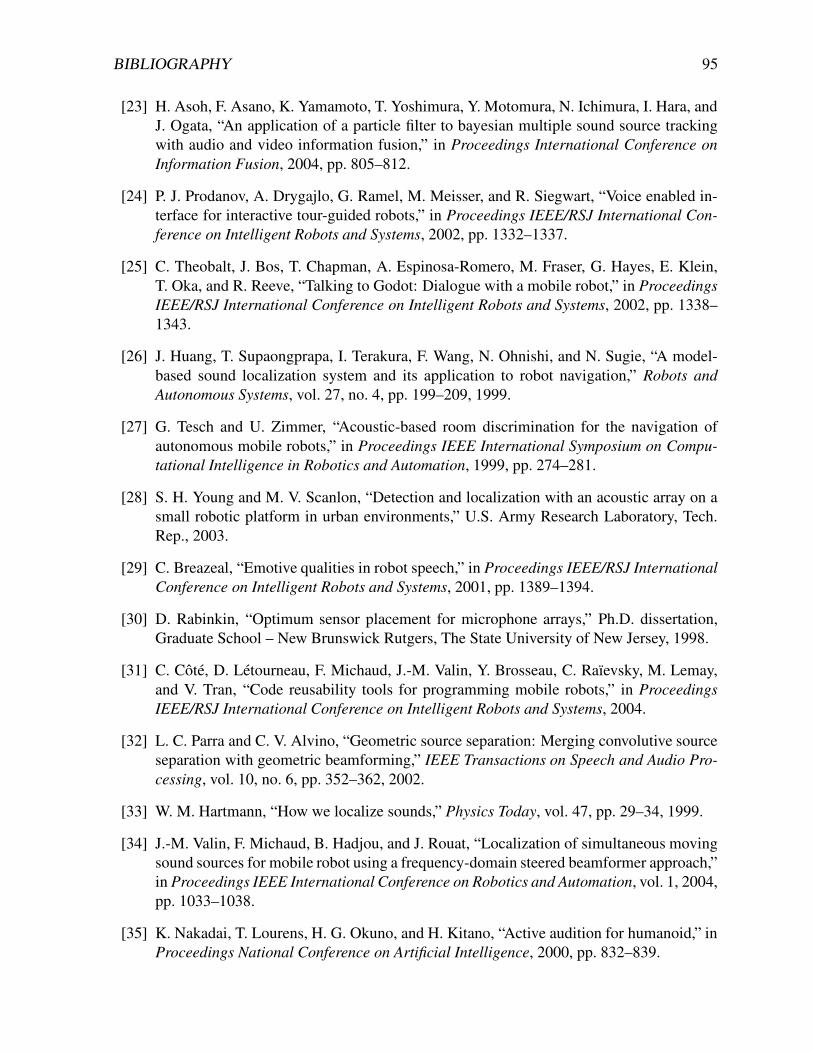
BIBLIOGRAPHY 95
[23] H. Asoh, F. Asano, K. Yamamoto, T. Yoshimura, Y. Motomura, N. Ichimura, I. Hara, andJ. Ogata, “An application of a particle filter to bayesian multiple sound source trackingwith audio and video information fusion,” in Proceedings International Conference onInformation Fusion, 2004, pp. 805–812.
[24] P. J. Prodanov, A. Drygajlo, G. Ramel, M. Meisser, and R. Siegwart, “Voice enabled in-terface for interactive tour-guided robots,” in Proceedings IEEE/RSJ International Con-ference on Intelligent Robots and Systems, 2002, pp. 1332–1337.
[25] C. Theobalt, J. Bos, T. Chapman, A. Espinosa-Romero, M. Fraser, G. Hayes, E. Klein,T. Oka, and R. Reeve, “Talking to Godot: Dialogue with a mobile robot,” in ProceedingsIEEE/RSJ International Conference on Intelligent Robots and Systems, 2002, pp. 1338–1343.
[26] J. Huang, T. Supaongprapa, I. Terakura, F. Wang, N. Ohnishi, and N. Sugie, “A model-based sound localization system and its application to robot navigation,” Robots andAutonomous Systems, vol. 27, no. 4, pp. 199–209, 1999.
[27] G. Tesch and U. Zimmer, “Acoustic-based room discrimination for the navigation ofautonomous mobile robots,” in Proceedings IEEE International Symposium on Compu-tational Intelligence in Robotics and Automation, 1999, pp. 274–281.
[28] S. H. Young and M. V. Scanlon, “Detection and localization with an acoustic array on asmall robotic platform in urban environments,” U.S. Army Research Laboratory, Tech.Rep., 2003.
[29] C. Breazeal, “Emotive qualities in robot speech,” in Proceedings IEEE/RSJ InternationalConference on Intelligent Robots and Systems, 2001, pp. 1389–1394.
[30] D. Rabinkin, “Optimum sensor placement for microphone arrays,” Ph.D. dissertation,Graduate School – New Brunswick Rutgers, The State University of New Jersey, 1998.
[31] C. Côté, D. Létourneau, F. Michaud, J.-M. Valin, Y. Brosseau, C. Raïevsky, M. Lemay,and V. Tran, “Code reusability tools for programming mobile robots,” in ProceedingsIEEE/RSJ International Conference on Intelligent Robots and Systems, 2004.
[32] L. C. Parra and C. V. Alvino, “Geometric source separation: Merging convolutive sourceseparation with geometric beamforming,” IEEE Transactions on Speech and Audio Pro-cessing, vol. 10, no. 6, pp. 352–362, 2002.
[33] W. M. Hartmann, “How we localize sounds,” Physics Today, vol. 47, pp. 29–34, 1999.
[34] J.-M. Valin, F. Michaud, B. Hadjou, and J. Rouat, “Localization of simultaneous movingsound sources for mobile robot using a frequency-domain steered beamformer approach,”in Proceedings IEEE International Conference on Robotics and Automation, vol. 1, 2004,pp. 1033–1038.
[35] K. Nakadai, T. Lourens, H. G. Okuno, and H. Kitano, “Active audition for humanoid,” inProceedings National Conference on Artificial Intelligence, 2000, pp. 832–839.

96 BIBLIOGRAPHY
[36] J.-M. Valin, F. Michaud, J. Rouat, and D. Létourneau, “Robust sound source localizationusing a microphone array on a mobile robot,” in Proceedings IEEE/RSJ InternationalConference on Intelligent Robots and Systems, 2003, pp. 1228–1233.
[37] S. Kagami, Y. Tamai, H. Mizoguchi, and T. Kanade, “Microphone array for 2D soundlocalization and capture,” in Proceedings IEEE International Conference on Roboticsand Automation, 2004, pp. 703–708.
[38] Q. Wang, T. Ivanov, and P. Aarabi, “Acoustic robot navigation using distributed micro-phone arrays,” Information Fusion (Special Issue on Robust Speech Processing), vol. 5,no. 2, pp. 131–140, 2004.
[39] D. Bechler, M. Schlosser, and K. Kroschel, “System for robust 3D speaker tracking usingmicrophone array measurements,” in Proceedings IEEE/RSJ International Conference onIntelligent Robots and Systems, 2004, pp. 2117–2122.
[40] M. S. Arulampalam, S. Maskell, N. Gordon, and T. Clapp, “A tutorial on particle fil-ters for online nonlinear/non-gaussian bayesian tracking,” IEEE Transactions on SignalProcessing, vol. 50, no. 2, pp. 174–188, 2002.
[41] D. B. Ward and R. C. Williamson, “Particle filtering beamforming for acoustic source lo-calization in a reverberant environment,” in Proceedings IEEE International Conferenceon Acoustics, Speech, and Signal Processing, vol. II, 2002, pp. 1777–1780.
[42] D. B. Ward, E. A. Lehmann, and R. C. Williamson, “Particle filtering algorithms fortracking an acoustic source in a reverberant environment,” IEEE Transactions on Speechand Audio Processing, vol. 11, no. 6, pp. 826–836, 2003.
[43] J. Vermaak and A. Blake, “Nonlinear filtering for speaker tracking in noisy and reverber-ant environments,” in Proceedings IEEE International Conference on Acoustics, Speech,and Signal Processing, vol. 5, 2001, pp. 3021–3024.
[44] J. Vermaak, A. Doucet, and P. Pérez, “Maintaining multi-modality through mixture track-ing,” in Proceedings International Conference on Computer Vision, 2003, pp. 1950–1954.
[45] J. MacCormick and A. Blake, “A probabilistic exclusion principle for tracking multipleobjects,” International Journal of Computer Vision, vol. 39, no. 1, pp. 57–71, 2000.
[46] C. Hue, J.-P. L. Cadre, and P. Perez, “A particle filter to track multiple objects,” inProceedings IEEE Workshop on Multi-Object Tracking, 2001, pp. 61–68.
[47] J. Vermaak, S. Godsill, and P. Pérez, “Monte Carlo filtering for multi-target tracking anddata association,” IEEE Transactions on Aerospace and Electronic Systems, 2005. (Toappear).
[48] R. Duraiswami, D. Zotkin, and L. Davis, “Active speech source localization by a dualcoarse-to-fine search,” in Proceedings IEEE International Conference on Acoustics,Speech, and Signal Processing, 2001, pp. 3309–3312.

BIBLIOGRAPHY 97
[49] M. Omologo and P. Svaizer, “Acoustic event localization using a crosspower-spectrumphase based technique,” in Proceedings IEEE International Conference on Acoustics,Speech, and Signal Processing, 1994, pp. II–273–II–276.
[50] Y. Ephraim and D. Malah, “Speech enhancement using minimum mean-square errorshort-time spectral amplitude estimator,” IEEE Transactions on Acoustics, Speech andSignal Processing, vol. ASSP-32, no. 6, pp. 1109–1121, 1984.
[51] I. Cohen and B. Berdugo, “Speech enhancement for non-stationary noise environments,”Signal Processing, vol. 81, no. 2, pp. 2403–2418, 2001.
[52] J. Huang, N. Ohnishi, and N. Sugie, “Sound localization in reverberant environmentbased on the model of the precedence effect,” IEEE Transactions on Instrumentationand Measurement, vol. 46, no. 4, pp. 842–846, 1997.
[53] J. Huang, N. Ohnishi, X. Guo, and N. Sugie, “Echo avoidance in a computational modelof the precedence effect,” Speech Communication, vol. 27, no. 3-4, pp. 223–233, 1999.
[54] B. Mungamuru and P. Aarabi, “Enhanced sound localization,” IEEE Transactions onSystems, Man, and Cybernetics Part B, vol. 34, no. 3, pp. 1526–1540, 2004.
[55] F. Giraldo, “Lagrange-Galerkin methods on spherical geodesic grids,” Journal of Com-putational Physics, vol. 136, pp. 197–213, 1997.
[56] A. Doucet, S. Godsill, and C. Andrieu, “On sequential Monte Carlo sampling methodsfor bayesian filtering,” Statistics and Computing, vol. 10, pp. 197–208, 2000.
[57] W. M. Hartmann, “Localization of sounds in rooms,” Journal of the Acoustical Society ofAmerica, vol. 74, pp. 1380–1391, 1983.
[58] B. Rakerd and W. M. Hartmann, “Localization of noise in a reverberant environment,” inProceedings International Congress on Acoustics, 2004.
[59] S. Haykin, Neural Networks, a Comprehensive Foundation, 2nd ed. Prentice Hall, 1999.
[60] J.-F. Cardoso, “Blind signal separation: Statistical principles,” in Proceedings IEEE,vol. 9, no. 10, 1998, pp. 2009–2025.
[61] H. Saruwatari, T. Kawamura, and K. Shikano, “Blind source separation for speech basedon fast-convergence algorithm with ica and beamforming,” in Proceedings Eurospeech,2001, pp. 2603–2606.
[62] A. Koutras, E. Dermatas, and G. Kokkinakis, “Improving simultaneous speech recogni-tion in real room environments using overdetermined blind source separation,” in Pro-ceedings Eurospeech, 2001, pp. 1009–1012.
[63] S. Araki, S. Makino, R. Mukai, and H. Saruwatari, “Equivalence between frequencydomain blind source separation and frequency domain adaptive null beamformers,” inProceedings Eurospeech, 2001, pp. 2595–2598.

98 BIBLIOGRAPHY
[64] R. Mukai, S. Araki, and S. Makino, “Separation and dereverberation performance offrequency domain blind source separation for speech in a reverberant environment,” inProceedings Eurospeech, 2001, pp. 2599–2602.
[65] S. Rickard, R. Balan, and J. Rosca, “Real-time time-frequency based blind source sep-aration,” in Proceedings International Conference on Independent Component Analysisand Blind Source Separation, 2001, pp. 651–656.
[66] S. Araki, S. Makino, A. Blin, R. Mukai, and H. Sawada, “Underdetermined blind sep-aration for speech in real environments with sparseness and ica,” in Proceedings IEEEInternational Conference on Acoustics, Speech, and Signal Processing, 2004, pp. 881–884.
[67] S.-I. Amari, A. Cichocki, and H. H. Yang, “Blind signal separation and extraction: Neu-ral and information-theoretic approaches,” in Unsupervised Adaptive Filtering volumeI, Blind Source Separation, ser. Adaptive and Learning Systems for Signal Processing.Wiley-Interscience, 2000, ch. 3, pp. 63–138.
[68] P. Comon and P. Chevalier, “Blind source separation: Models, concepts, algorithms, andperformance,” in Unsupervised Adaptive Filtering Volume I, Blind Source Separation,ser. Adaptive and Learning Systems for Signal Processing. Wiley-Interscience, 2000,ch. 5, pp. 191–235.
[69] S. Haykin, Adaptive Filter Theory, 4th ed. Prentice Hall, 2002.
[70] L. J. Griffiths and C. W. Jim, “An alternative approach to linearly constrained adaptivebeamforming,” IEEE Transactions on Antennas and Propagation, vol. AP-30, no. 1, pp.27–34, 1982.
[71] S. Gannot, D. Burshtein, and E. Weinstein, “Signal enhancement using beamforming andnonstationarity with application to speech,” IEEE Transactions on Signal Processing,vol. 49, no. 8, pp. 1614–1626, 2001.
[72] O. Hoshuyama, A. Sugiyama, and A. Hirano, “A robust adaptive beamformer for micro-phone arrays with a blocking matrix using constrained adaptive filters,” IEEE Transac-tions on Signal Processing, vol. 47, no. 10, pp. 2677–2684, 1999.
[73] M. S. Pedersen and L. K. Hansen, “Semi-blind source separation using head-relatedtransfer functions,” in Proceedings IEEE International Conference on Acoustics, Speech,and Signal Processing, vol. V, 2004, pp. 713–716.
[74] S. F. Boll, “A spectral subtraction algorithm for suppression of acoustic noise in speech,”in Proceedings IEEE International Conference on Acoustics, Speech, and Signal Pro-cessing, 1979, pp. 200–203.
[75] Y. Ephraim and D. Malah, “Speech enhancement using minimum mean-square errorlog-spectral amplitude estimator,” IEEE Transactions on Acoustics, Speech and SignalProcessing, vol. ASSP-33, no. 2, pp. 443–445, 1985.

BIBLIOGRAPHY 99
[76] R. Zelinski, “A microphone array with adaptive post-filtering for noise reduction in re-verberant rooms,” in Proceedings IEEE International Conference on Acoustics, Speech,and Signal Processing, vol. 5, 1988, pp. 2578–2581.
[77] I. McCowan, C. Marro, and L. Mauuary, “Robust speech recognition using near-field su-perdirective beamforming with post-filtering,” in Proceedings IEEE International Con-ference on Acoustics, Speech, and Signal Processing, 2000, p. 1723.
[78] I. McCowan and H. Bourlard, “Microphone array post-filter for diffuse noise field,” inProceedings IEEE International Conference on Acoustics, Speech, and Signal Process-ing, vol. 1, 2002, pp. 905–908.
[79] I. Cohen and B. Berdugo, “Microphone array post-filtering for non-stationary noise sup-pression,” in Proceedings IEEE International Conference on Acoustics, Speech, and Sig-nal Processing, 2002, pp. 901–904.
[80] J.-M. Valin, J. Rouat, and F. Michaud, “Enhanced robot audition based on microphonearray source separation with post-filter,” in Proceedings IEEE/RSJ International Confer-ence on Intelligent Robots and Systems, 2004, pp. 2123–2128.
[81] I. Cohen, “On the decision-directed estimation approach of Ephraim and Malah,” in Pro-ceedings IEEE International Conference on Acoustics, Speech, and Signal Processing,2004, pp. 293–296.
[82] J.-M. Valin, J. Rouat, and F. Michaud, “Microphone array post-filter for separation ofsimultaneous non-stationary sources,” in Proceedings IEEE International Conference onAcoustics, Speech, and Signal Processing, 2004.
[83] M. Wu and D. Wang, “A two-stage algorithm for enhancement of reverberant speech,” inProceedings IEEE International Conference on Acoustics, Speech, and Signal Process-ing, 2005, pp. 1085–1088.
[84] M. S. Choi and H. G. Kang, “An improved estimation of a priori speech absence prob-ability for speech enhancement : in perspective of speech perception,” in ProceedingsIEEE International Conference on Acoustics, Speech, and Signal Processing, 2005, pp.1117–1120.
[85] D. Pearce, “Developing the ETSI Aurora advanced distributed speech recognition front-end & what next,” in Proceedings IEEE Automatic Speech Recognition and Understand-ing Workshop, 2001.
[86] P. Aarabi and G. Shi, “Phase-based dual-microphone robust speech enhancement,” IEEETransactions on Systems, Man and Cybernetics, vol. 34, no. 4, pp. 1763–1773, 2004.
[87] F. Asano, M. Goto, K. Itou, and H. Asoh, “Real-time sound source localization andseparation system and its application to automatic speech recognition,” in ProceedingsEurospeech, 2001, pp. 1013–1016.

100 BIBLIOGRAPHY
[88] K. Nakadai, H. G. Okuno, and H. Kitano, “Auditory fovea based speech separation andits application to dialog system,” in Proceedings IEEE/RSJ International Conference onIntelligent Robots and Systems, 2002, pp. 1314–1319.
[89] P. Renevey, R. Vetter, and J. Kraus, “Robust speech recognition using missing featuretheory and vector quantization,” in Proceedings Eurospeech, 2001, pp. 1107–1110.
[90] J. Barker, L. Josifovski, M. Cooke, and P. Green, “Soft decisions in missing data tech-niques for robust automatic speech recognition,” in Proceedings IEEE International Con-ference on Spoken Language Processing, vol. I, 2000, pp. 373–376.
[91] S. Yamamoto, J.-M. Valin, K. Nakadai, J. Rouat, F. Michand, T. Ogata, and H. G. Okuno,“Enhanced robot speech recognition based on microphone array source separation andmissing feature theory,” in Proceedings IEEE International Conference on Robotics andAutomation, 2005, pp. 1489–1494.
[92] R. P. Lippmann, E. A. Martin, and D. B. Paul, “Multi-styletraining for robust isolated-word speech recognition,” in Proceedings IEEE International Conference on Acoustics,Speech, and Signal Processing, 1987, pp. 705–708.
[93] M. Blanchet, J. Boudy, and P. Lockwood, “Environment adaptation for speech recogni-tion in noise,” in Proceedings European Signal Processing Conference, vol. VI, 1992, pp.391–394.
[94] D. O’Shaughnessy, “Interacting with computers by voice: automatic speech recognitionand synthesis,” Proceedings of the IEEE, vol. 91, no. 9, pp. 1272–1305, Sept. 2003.
[95] M. L. Seltzer and R. M. Stern, “Subband parameter optimization of microphone arraysfor speech recognition in reverberant environments,” in Proceedings IEEE InternationalConference on Acoustics, Speech, and Signal Processing, 2003, pp. 408–411.
[96] M. Cooke, P. Green, and M. Crawford, “Handling missing data in speech recognition,”in Proceedings IEEE International Conference on Spoken Language Processing, 1994,Paper 26.20.
[97] M. Cooke, P. Green, L. Josifovski, and A. Vizinho, “Robust automatic speech recognitionwith missing and unreliable acoustic data,” Speech Communication, vol. 34, pp. 267–285,2001.
[98] J. Barker, M. Cooke, and P. Green, “Robust ASR based on clean speech models: Anevaluation of missing data techniques for connected digit recognition in noise,” in Pro-ceedings Eurospeech, 2001, pp. 213–216.
[99] J. Picone, “Signal modeling techniques in speech recognition,” IEEE Proceedings,vol. 81, no. 9, pp. 1215–1247, 1993.
[100] H. V. hamme, “Robust speech recognition using missing feature theory in the cepstral orLDA domain,” in Proceedings Eurospeech, 2003, pp. 1973–1976.

BIBLIOGRAPHY 101
[101] ——, “Robust speech recognition using cepstral domain missing data techniques andnoisy masks,” in Proceedings IEEE International Conference on Acoustics, Speech, andSignal Processing, 2004, pp. 213–216.
[102] B. Raj, M. L. Seltzer, and R. M. Stern, “Reconstruction of missing features for robustspeech recognition,” Speech Communication, vol. 43, no. 4, pp. 275–296, 2004.
[103] M. L. Seltzer, B. Raj, and R. M. Stern, “A bayesian framework for spectrographic maskestimation for missing feature speech recognition,” Speech Communication, vol. 43,no. 4, pp. 379–393, Sept 2004.
[104] J. Ming, P. Jancovic, and F. J. Smith, “Robust speech recognition using probabilisticunion models,” IEEE Transactions on Speech and Audio Processing, vol. 10, no. 6, pp.403–414, 2002.
[105] J. Ming and F. J. Smith, “Speech recognition with unknown partial feature corruption –a review of the union model,” Computer Speech and Language, vol. 17, pp. 287–305,2003.
[106] H.-Y. Cho and Y.-H. Oh, “On the use of channel-attentive MFCC for robust recognition ofpartially corrupted speech,” IEEE Signal Processing Letters, vol. 11, no. 6, pp. 581–584,2004.
[107] I. McCowan, A. Morris, and H. Bourlard, “Improved speech recognition performance ofsmall microphone arrays using missing data techniques,” in Proceedings IEEE Interna-tional Conference on Spoken Language Processing, 2002, pp. 2181–2184.
[108] S. D. Peters, P. Stubley, and J.-M. Valin, “One the limits of speech recognition in noise,”in Proceedings IEEE International Conference on Acoustics, Speech, and Signal Pro-cessing, 1999, pp. 365–368.
[109] A. Lee, T. Kawahara, and K. Shikano, “Julius – An open-source real-time large vocabu-lary recognition engine,” in Proceedings Eurospeech, 2001, pp. 1691–1694.
[110] I. Zeljkovic and S. Narayanan, “Improved hmm phone and triphone models for real-timeasr telephony applications,” in Proceedings IEEE International Conference on SpokenLanguage Processing, vol. 2, 1996, pp. 1105–1108.
[111] L. Deng, J. Droppo, and A. Acero, “Exploiting variances in robust feature extractionbased on a parametric model of speech distortion,” in Proceedings IEEE InternationalConference on Spoken Language Processing, 2002, pp. 2449–2452.
[112] J. Droppo, A. Acero, and L. Deng, “Uncertainty decoding with SPLICE for noise ro-bust speech recognition,” in Proceedings IEEE International Conference on Acoustics,Speech, and Signal Processing, 2002, pp. 57–60.
[113] R. Pichevar, J. Rouat, C. Feldbauer, and G. Kubin, “A bio-inspired sound source sep-aration technique based on a spiking neural network in combination with an enhancedanalysis/synthesis filterbank,” in Proceedings European Signal Processing Conference,2004.

102 BIBLIOGRAPHY
[114] S. Pfeiffer, C. Parker, and C. Schremmer, “Annodex: a simple architecture to enablehyperlinking, search & retrieval of time–continuous data on the web,” in ProceedingsACM SIGMM International Workshop on Multimedia Information Retrieval, 2003, pp.87–93.


