University of Toronto Department of Economics
January 30, 2008
By Andreas Park
Bid-Ask Spreads and Volume:The Role of Trade Timing
Working Paper 309
Bid-Ask Spreads and Volume:
The Role of Trade Timing
Andreas Park∗
University of Toronto
January 29, 2008
Abstract
I formulate a stylized Glosten-Milgrom model of financial market trading in
which people are allowed to time their trading decision. The focus of the analysis is
to understand people’s timing behavior and how it affects bid- and offer-prices and
volume. Assuming heterogeneous quality of information, not all informed traders
choose to trade immediately but some chose to delay, although they expect public
expectations to move against them. Compared to a myopic, no-timing setting, first
movers with timing have better quality information. Contrary to casual intuition
this behavior lowers bid-ask spreads early on and increases them in later periods.
Price-variability and total volume in both periods combined decrease. A numerical
analysis shows that with timing the spreads are very stable (though decreasing),
and that volume is increasing over time. Moreover, with timing the probability of
informed trading (PIN) increases between periods.
JEL Classification: C70, D80, D82, D84, G14.
Keywords: Microstructure, Sequential Trade, Trade timing.
∗Financial support from the EU Commission (TMR grant number HPMT-GH-00-00046-08) is grate-fully acknowledged. Part of this project was done while I was at the University of Copenhagen, whichI thank for its hospitality. I also thank Bruno Biais, Li Hao, Rosemary (Gui Ying) Luo, Katya Ma-linova, Angelo Melino, Jordi Mondria, and Peter Norman Sørensen for helpful comments. Email:[email protected]; web: http://www.chass.utoronto.ca/∼apark/
1 Introduction
One persistent finding in empirical market microstructure is that volume and spreads
display intra-day patterns. These patterns have different shapes across markets and
across the time periods studied, but all in all systematic patterns exist and persist,1 the
most common being that spreads decline through the day and that volume increases
towards the end of the day. While there are some (theoretical) explanations for these
patterns, no published paper employs a Glosten and Milgrom (1985) (henceforth GM)
style formulation to study timing and bid-ask spread patterns — even though this kind
of model should be the natural choice to study spreads. In this paper I will demonstrate
that traders’ behavior in such a GM model with strategic timing of trades naturally
generates a large part of the commonly observed patterns.
In my simple framework with endogenous timing of unit trades investors not only
choose whether to buy or sell, but also when to trade. The purpose of the analysis is
to understand the timing behavior of individuals and that effects that this behavior has
on the observables, namely prices and volume. I employ a stylized version of Glosten
and Milgrom’s sequential trading model with two periods, two investors, two liquidation
values, and a continuum of signals. Prices are set by competitive market makers.
In equilibrium better informed investors trade early, and less-well informed trade
late. This implies that people with private information delay even though they expect
the public expectation to move against them (e.g. someone with favorable information
expects the public expectation to rise). Moreover, compared to a no-timing scenario,
fewer people trade early (and thus more delay). This behavior affects the observables
by decreases in the bid-ask-spread early on, and by increasing the spread later on which
thus goes hand-in-hand with a reduction in price variability. Total volume is lower in
the setting with timing, and the pattern of volume across time is reversed: with timing,
volume is low early-on and large later-on, without timing it is the reverse.
Patterns in trading variables suggest non-stationary behavior. For my study of trade-
timing, I employ the most frequently used, stylized formulation of the GM sequential
1The most common pattern for NYSE is that spreads and volume are U- or reverse J-shaped; see,for instance, Jain and Joh (1988), Brock and Kleidon (1992), McInish and Wood (1992), Lee, Mucklow,and Ready (1993), or Brooks, Hinich, and Patterson (2003). There is some recent evidence, however,that the spread-pattern may have morphed to an L-shape after decimalization; see Serednyakov (2005).On Nasdaq spreads are L-shaped and volume is U-shaped; see, for instance, Chan, Christie, and Schultz(1995). On the London Stock Exchange, spreads are L-shaped and volume reverse-L-shaped, with twosmall humps during the day; see Kleidon and Werner (1996) or Cai, Hudson, and Keasey (2004). Otherworld markets, for instance, the Taiwan and the Singapore Stock exchanges have L-shaped spreadsand reverse L-shaped volume/number of transactions; for Taiwan, see Lee, Fok, and Liu (2001); forSingapore see Ding and Lau (2001).
1 The Timing of Trades
trading model and amend it slightly to allow non-stationarity, strategic behavior in that
some people are allowed to time their actions. In said standard models traders arrive
according to a random sequence, and trade exactly at the time of their arrival. Some
traders are informed, having received a single private signal about the true value of the
underlying asset, others are noise and trade for reasons outside of the model such as
liquidity.2 A risk-neutral, perfectly competitive market maker sets a bid-price at which
she is willing to sell and an ask price at which she is willing to buy. Each of these prices
anticipates the informational content of the upcoming trade, thus generating a spread
between the bid- and the ask price.
In the model presented in this paper, two traders enter the market before the first
period and they can then choose whether to trade in period one or two. This allows me
to study a stylized timing decision for a very short-run setting. Loosely, one could take
the two periods of trading as the morning and afternoon sessions. Also, the presence
of competition between traders suggests information that has a relatively short half-life
(e.g. it is based on an upcoming announcement).
Next, most GM models use a single kind of binary signal; while in my model informed
traders also receive binary signals, these signals come in a continuum of precisions and
an informed trader is thus associated with the precision (or quality) of his binary signal.3
This effectively induces a continuous signal structure and allows a simple and concise
characterization of the equilibrium by marginal trading types. These marginal types
are indifferent between trading immediately and delaying.4 Employing symmetry with
respect to the prior distribution of the security values and the signal distribution (as is
common in the literature), I then establish the existence of a trading equilibrium.
At the heart of the paper is the comparison of the size of bid-ask-spreads and overall
volume for cases with and without timing. Since bid-ask spreads are employed in most
measures of market liquidity, it is of some importance to understand how traders time
their trading decision in an attempt to exploit liquidity and to manage transaction costs.
As the no-timing benchmark I employ a hypothetical setting in which agents do not time
their trade and instead behave purely myopically.5
2See, e.g., Easley and O’Hara (1987), or Avery and Zemsky (1998).3This information structure is commonly used in informational learning models, see, for instance,
Smith and Sørensen (2000).4On a theoretical level, this is a ‘purification’ approach: standard stylized GM models use only a
single signal. To study meaningful information-induced delay, I would have to include at least two kindsof signal (e.g. high and low quality; as also used in Easley and O’Hara (1987)). This, however, wouldinvariably force me to describe behavior by mixed strategies. The continuous signal space not onlyallows me to circumvent this complication, but it also delivers cleaner insights (mixed strategies can bedifficult to interpret).
5When prompted to trade, such traders simply ignore the possibility of delay. For instance, such
2 The Timing of Trades
In equilibrium, there are two forces at play: first, informed traders believe that the
market will move against them. Traders with favorable information expect the public
expectation (the market) to rise, traders with unfavorable information expect the public
expectation to fall.6 Delaying for this reason can be interpreted as causing a type II
error (not buying a valuable security, not selling an overpriced security). The public
expectation is not, however, the measure that determines traders’ payoffs — trades occur
at bid- and offer-prices (which underlines to importance of using a GM formulation).
This gives rise to the second force: Suppose, for the sake of the argument, that in Period 1
people with very high quality information buy or sell and that people with low quality
information choose not to trade.7 In Period 2, the market maker would know that she
is only facing agents with low quality information, and so there is less of a reason to
defend against the potential informational advantage of the remaining informed traders.
Consequently, the bid-ask-spread in the second period would be smaller. In equilibrium
there is a unique marginal type who is indifferent between trading in Period 1 and 2.
In stationary binary states Glosten-Milgrom models, the bid- and ask prices merely
separate people with favorable information (who buy) from those with unfavorable infor-
mation (who sell). With timing, the adjustments of the spread across time also separate
people with stronger and weaker information on the same side of the market.8
To understand the impact of timing on the equilibrium behavior I then compare the
timing equilibrium with a situation in which traders have no strategic timing consider-
ations. The first result is that the marginal trader in the no-timing (myopic) situation
who is indifferent between trading early or never, strictly prefers to delay with timing.
In other words, in equilibrium the marginal trading type in a myopic setting has a lower
signal quality than in the setting with strategic timing. Consequently, in the equilibrium
with timing the average signal quality of informed traders who move early is larger, and
thus traders need relatively better information in order to trade early.
It may appear at first sight that with timing the bid-ask spread in the first period
should be larger relative to the no-timing situation. This intuition, however, is mislead-
ing: the size of the bid-ask spread depends on the extent of informed trading. While
each informed trade is more informative, people who have this high quality signal are
traders may arrive at the market in the morning, check prices, and decide not to trade. In the afternoon,they take a second look, and then may reconsider, even though they hadn’t planned on it.
6More technically, the public expectation follows a martingale process, but the expectation of anytrader with favorable information about this public expectation follows a submartingale, that of a traderwith unfavorable information follows a supermartingale.
7Those who trade then have either a very favorable or a very unfavorable opinion about the asset.8As Malinova and Park (2008) show, different trade sizes in an anonymous market, for instance,
cannot easily accomplish this feat.
3 The Timing of Trades
rare. And so for any trade, the relative likelihood of informed trading relative to unin-
formed trading is smaller in the timing setting. This causes the timing bid-ask-spread
in the first period to be smaller than the myopic spread. In the second period, how-
ever, the opposite occurs: the bid-ask-spread with timing is wider than without timing.
Since the spread between periods declines, prices with timing are actually more stable.
Moreover, with timing total volume will be smaller because the overall proportion of
informed insiders who trade is smaller.
While short of an analytical result, patterns in volume are unambiguously reflected
in numerical simulations.9 Volume patterns with and without timing are strikingly
different: with timing, volume is small early and large later, whereas without timing it
is the other way round. The intuition behind the volume patterns can be deduced from
the bid-ask-spreads: in the timing equilibrium, early- and late-moving incentives must
be balanced for a marginal type. This balancing ensures that, by-and-large, spreads
are similar in both periods. Also, spreads are, loosely speaking, proportional to the
product of the average signal quality with the probability mass of traders who have this
signal quality. Since the average quality in Period 1 is high and in Period 2 lower, the
probability mass has to be low first and then high, giving rise to the volume pattern.
With myopic behavior, spreads screen out a similar proportion of signal qualities in each
period; since the size of remaining set declines, so will the volume. While my model is
too stylized to make sweeping claims about being a full explanation for volume patterns,
it tells a conclusive story as to why an increase in volume over time may arise as an
equilibrium phenomenon. My results are thus an important first step in understanding
such patterns theoretically.
The volume-spread simulations can straightforwardly be extended to capture another
common empirical microstructure measure: the probability of informed trading, PIN.
The concept was first employed by Easley, Kiefer, O’Hara, and Paperman (1996) and it
estimates the probability that a trade is initiated by an informed insider. In line with the
results outlined above, analytically, PIN in Period 1 is larger in the myopic case. This
alone gives no testable implication, but simulations provide a new testable hypothesis:
simulations show that with timing PIN actually increases from Period 1 to Period 2,
whereas with myopic behavior, PIN decreases from Period 1 to Period 2.10
9These simulations were run for a quadratic and a symmetric Beta distribution over signal qualities.The computation was run in Maple; the underlying code is available upon demand.
10Several authors, e.g. Lin, Sanger, and Booth (1995), Madhavan, Richardson, and Roomans (1997),or Serednyakov (2005), have ventured to empirically decompose the spread into informational, orderprocessing, and inventory costs (for NYSE) and they find that the informational cost is higher early onwhereas inventory costs are high later on. Lee, Fok, and Liu (2001) find that insiders and noise traderssubmit more trades at the open and the close. Comerton-Forde, O’Brian, and Westerholm (2004), on
4 The Timing of Trades

Related Theoretical Literature on Timing in Markets. There is a substan-
tial body of literature that studies repeated trading in either Kyle-type or in rational
expectations equilibria (REE) type settings. Neither of these frameworks, however, is
well-suited to study bid-ask-spreads. Moreover, on a conceptual level these models cap-
ture a different market microstructure, namely (batch) auctions or order-driven markets
with simultaneous moves; GM models, on the other hand, capture quote-driven mar-
kets.11 There is also a reasonably large body of literature on the timing of investments,
e.g. Chamley and Gale (1994), Gul and Lundholm (1995) Chari and Kehoe (2004),
Lee (1998), Abreu and Brunnermeier (2003), but these papers are not concerned with
standard market microstructure measures such as volume, the probability of informed
trading, liquidity, or bid-ask-spreads.
To the best of my knowledge, there are only two published papers that extend Glosten
and Milgrom’s seminal model to allow endogenous timing: Back and Baruch (2004) and
Chakraborty and Yilmaz (2004a). Both of these, however, model a single informed
insider who can trade repeatedly. Back and Baruch’s focus is to show that in the limit,
the equilibrium from a Glosten-Milgrom setting converges to the equilibrium in a Kyle
model. Chakraborty and Yilmaz analyze if the single insider can effectively manipulate
the market. In my paper, the competition between two potentially informed traders
is the mechanism that creates the delay/early-play trade-offs, because rational traders
anticipate the direction of future prices. Studying manipulative strategies, such as those
described in Chakraborty and Yilmaz (2004a), would go beyond the scope of this paper
and thus manipulation plays no role here.
Finally, Smith (2000) has a similar financial market setting, but without a market
maker who sets bid- and ask-prices and without the informed trade having an impact
on the price. Then in Smith, an investor with private information trades early. The
intuition is, of course, that someone with, say, a favorable signal expects transaction
prices to increase (for him it is a sub-martingale). Casual intuition then suggests, that
profits from speculation are largest early so that investors should invest rather earlier
the other hand, find that the proportion of informed traders tend to increase throughout the day. I amnot aware, however, of any study that estimates intra-day patterns in PIN directly.
11In Kyle (1985), a market maker sets the price after observing the aggregate order flow (whichconsists entirely of market orders), and so this procedure rather mimics the opening sessions at NYSEor Deutsche Borse. Likewise, REE setups, most famously Admati and Pfleiderer (1988), require thattraders submit (complete) demand-supply schedules and so an REE setting mimics opening sessions asheld at the TSX or Paris Bourse; in an REE setup, however, spreads are not modeled explicitly. Toexplain patterns in volume and spreads, there are also models that are not information-based in whichone determines the optimal behavior against exogenous, periodic occurrences of the supply of tradingparties (see Brock and Kleidon (1992)). At the same time, one usually uses a GM sequential tradingframework when modeling continuous trading.
5 The Timing of Trades
than later. My result is somewhat surprising as it indicates the opposite: the type who
is the marginal buyer without timing would delay the purchase with timing because
he would expect the future ask-prices to fall — despite his favorable information. The
difference between our setups are that Smith has no bid-ask-spread and that market
prices in his model do not account for the (timing) behavior of the informed agent.
The paper proceeds as follows: in the next section I outline the basic model, in
particular, the information structure, and I discuss some key assumptions of the model.
In Section 3 I derive the equilibria for the timing and the no-timing cases. The discussion
and comparison of these equilibria follows in Section 4. Their respective price-, volume-
and PIN-implications are discussed in Sections 5, 6, and 7. Section 8 discussed the
results and concludes. Appendix A contains some further numerical robustness checks.
Appendix B provides the more technical details of the signal structure. All proofs are
delegated to Appendix C.
2 The Basic Setup
I formulate a stylized version of security trading in which informed and uninformed
investors trade unit lots of a single asset with competitive market makers. There are
two investors who can trade either in Period 1 or Period 2; each can trade at most
once. Informed investors receive information about the true state of the asset before
time 1, whereas uninformed investors trade for liquidity reasons. After time 2, the true
value of the security will be revealed. Short positions are filled at the true value. Each
market maker posts a bid-price at which she is willing to buy the security and an offer-
price (‘ask’) at which she is willing to sell.12 Market makers are competitive and thus
set prices at which they make zero expected profits. After receiving their information,
informed traders try to predict the transaction price in Period 2 and thus determine
whether it is worthwhile to submit a market order in Period 1 (at the posted price) or
whether they should delay until the second period. In every period, orders are submitted
simultaneously. After Period 1, all trading activity is published. No trading occurs after
Period 2.
2.1 The Security, Investors, and the Trading Mechanism
Security: There is a single risky asset with a liquidation value V from a set of two
potential values V = {V , V } ≡ {0, 1}. The two values are equally likely.
12Throughout the paper I will refer to market makers as female and investors as male.
6 The Timing of Trades
Investors: There is an infinitely large pool of investors out of which two are
drawn at random before Period 1. Each investor is equipped with private information
with probability µ > 0; if not informed, an investor becomes a noise trader (probability
1−µ). The informed investors (also referred to as insiders) are risk neutral and rational.
Noise traders have no information and trade randomly. These investors are not
necessarily irrational, but they trade for reasons outside of this model, such as liquidity.13
I assume that they buy and sell in every period with equal probability, e.g. the probability
of a noise trader buy in each period is (1 − µ)/4 =: λ.14
I will use the terms ‘trader’ and ‘investor’ interchangeably; likewise I will use the
terms ‘informed investor’, ‘informed trader’ and ‘insider’ interchangeably.
Each investor can buy or sell one round lot (one unit)15 of the security at prices deter-
mined by the market maker, or he can be inactive (‘hold’). As in Glosten and Milgrom
(1985), each investor can trade only once. Investors can post only market orders. The
possible actions are thus {{buy in 1, hold in 2}, {hold in 1, buy in 2}, {hold in 1, sell in 2},
{sell in 1, hold in 2}, and {hold in 1, hold in 2}. Insiders choose an action to maximize
their expected trading profits.
Market and timing: There are two trading periods, t = 1, 2. Loosely, one
could understand these periods as the morning and the afternoon trading sessions. Both
investors enter the market before time 1 and they leave the market after time 2. There
is a continuum of market makers, all are risk neutral and competitive. Since there is
a continuum of market makers, the probability of submitting the order to the same
market maker is zero. I assume that the market makers post identical prices so that if
two traders submit the same order at the same time, they also pay the same price. As a
consequence, similarly to GM, when submitting their market order investors know the
price at which their order will clear; this is also in line with the usual perception that
market orders have no or hardly any price risk.
13Assuming the presence of noise traders is common practice in the literature on micro-structure withasymmetric information to prevent “no-trade” outcomes a la Milgrom-Stokey (1982).
14The results in this paper are robust to noise traders who abstain from trading entirely with positiveprobability or who trade with different probabilities in the two periods.
15This single unit assumption is standard in GM models and needed when with risk neutral traders.Allowing traders to act repeatedly would be contrary to the goal of the model of removing stationarityof behavior. To see this consider a risk-neutral traders with perfect information (see below). This traderwould like to trade as much and as often as he can. Thus allowing traders to act in both periods wouldremove the timing motive and thus lead to a stationary model. In summary, one should think of tradersas being sufficiently credit constrained so that indeed they can trade at most once.
7 The Timing of Trades
2.2 Information
The structure of the model is common knowledge among all market participants.16 The
identity of an investor and his signal are private information, but everyone can observe
past trades and transaction prices. The public information at the beginning of Period 2
lists the buys and sales in Period 1 together with the realized transaction prices.
Market maker. The market maker only has public information; she observes all
trades and no-trades.
Insiders’ information. I follow most of the GM literature and assume that in-
vestors receive a binary signal, h or l, about the true liquidation value V . These signals
are independently distributed, conditional on the true value V . In contrast to most of
the GM literature, I assume that these signals come in a continuum of qualities. Specif-
ically, insider i is told one of two possible, statistically true statements: ‘with chance qi,
the liquidation value is High/Low (h/l)’. This qi is the signal quality. The distribution
of qualities is independent of the asset’s true value and can be understood as reflecting,
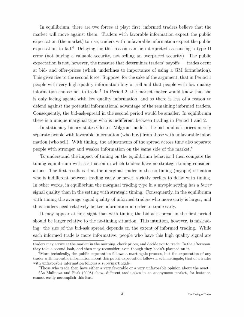
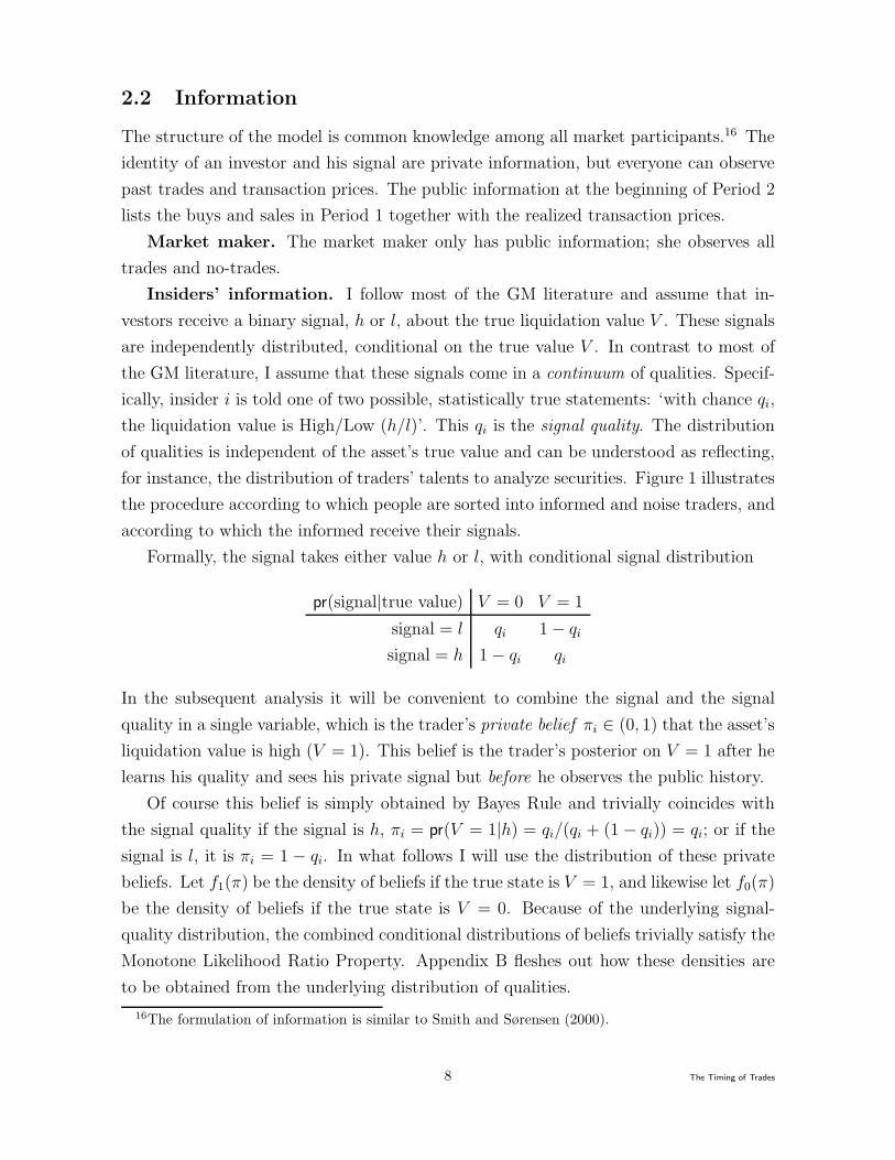
for instance, the distribution of traders’ talents to analyze securities. Figure 1 illustrates
the procedure according to which people are sorted into informed and noise traders, and
according to which the informed receive their signals.
Formally, the signal takes either value h or l, with conditional signal distribution
pr(signal|true value) V = 0 V = 1
signal = l qi 1 − qi
signal = h 1 − qi qi
In the subsequent analysis it will be convenient to combine the signal and the signal
quality in a single variable, which is the trader’s private belief πi ∈ (0, 1) that the asset’s
liquidation value is high (V = 1). This belief is the trader’s posterior on V = 1 after he
learns his quality and sees his private signal but before he observes the public history.
Of course this belief is simply obtained by Bayes Rule and trivially coincides with
the signal quality if the signal is h, πi = pr(V = 1|h) = qi/(qi + (1 − qi)) = qi; or if the
signal is l, it is πi = 1 − qi. In what follows I will use the distribution of these private
beliefs. Let f1(π) be the density of beliefs if the true state is V = 1, and likewise let f0(π)
be the density of beliefs if the true state is V = 0. Because of the underlying signal-
quality distribution, the combined conditional distributions of beliefs trivially satisfy the
Monotone Likelihood Ratio Property. Appendix B fleshes out how these densities are
to be obtained from the underlying distribution of qualities.
16The formulation of information is similar to Smith and Sørensen (2000).
8 The Timing of Trades
informed
noise
V = 1
V = 0
V = 1
V = 0
signal = h
signal = l
signal = h
signal = l
buy in 1
buy in 2
sell in 2
sell in 1
buy in 1
buy in 2
sell in 2
sell in 1
µ
1 − µ
signal qualitydistribution
signal qualitydistribution
1
2
1
2
qi
1− qi
1−qi
qi
1
2
1
2
1
4
1
4
1
4
1
4
1
4
1
4
1
4
1
4
signalquality
q i
Figure 1: Illustration of signals and noise. This figure illustrates how signals are distributed toinvestors: first, for each investor it is determined whether or not this trader is informed (probability µ)or noise (probability 1−µ). If informed, each trader i receives a draw of the signal quality is determinedaccording to the signal quality distribution. Depending on whether the state is high or low, the investorreceives the correct signal with probability qi and the wrong signal with probability 1− qi. (Of course,the draw of the state V is identical for all agents.) If the trader is a noise trader, then he will buy orsell with equal probability in either period.
9 The Timing of Trades
2
1
f1
f0
1
1
F1
F0
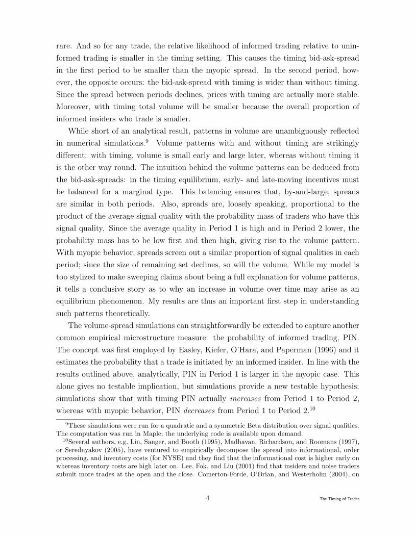
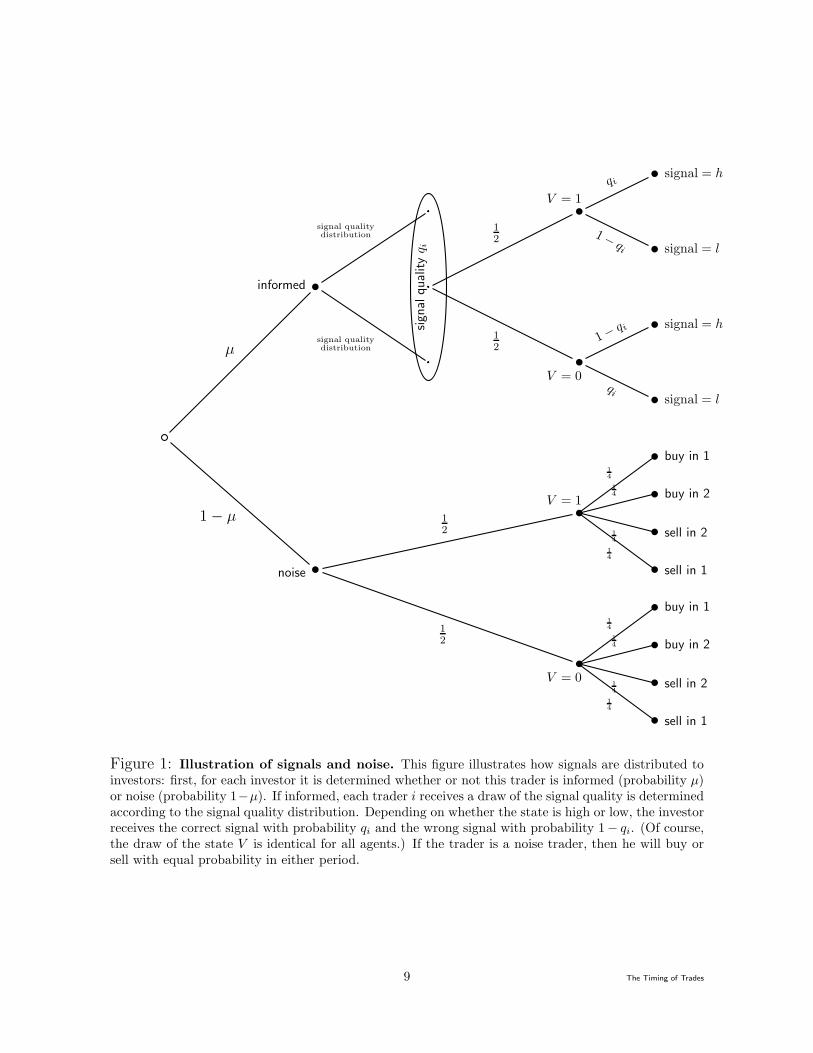
Figure 2: Plots of belief densities and distributions. Left Panel: The densities of beliefs for anexample with uniformly distributed qualities. The densities for beliefs conditional on the true state beingV = 1 and V = 1 respectively are f1(π) = 2π and f0(π) = 2(1 − π); Right Panel: The correspondingconditional distribution functions : F1(π) = π2 and F0(π) = 2π − π2.
Example of private beliefs. Figure 2 depicts an example where the signal
quality q is uniformly distributed. Conditional densities are f1(π) = 2π and f0(π) =
2(1 − π), yielding distributions F1(π) = π2 and F0(π) = 2π − π2. The figure also
illustrates the important principle that signals are informative: recipients in favor of
state V = 0 are more likely to occur in state V = 0 than in state V = 1.
2.3 The Trading Equilibrium
I assume that simultaneously submitted orders clear at the same transaction price, and
that investors who submit orders simultaneously do not observe each other’s actions.
Consequently, as in GM, when posting the order, an investor knows the price at which
his order will transact.
Equilibrium concept. The game played is one of incomplete information, the ap-
propriate equilibrium concept is thus the Perfect Bayesian Nash equilibrium. Henceforth
an equilibrium refers to a profile of actions for each type of insider that constitutes a
Perfect Bayesian equilibrium of the game. The price set by the market maker given
insiders’ action profiles is referred to as the equilibrium price. I will restrict attention to
symmetric equilibria, where all insiders use the same threshold decision rule.
The pricing rule: Market makers are competitive and make zero expected profits.
At each time t they post a bid- and an ask-price; the bid-price bidt is the price at which
they buy one unit of the security, the ask-price askt is the price at which they sell one
unit. With zero expected profits, for that trade it must hold that
askt = E[V |buy at askt, public info at t], bidt = E[V |sale at bidt, public info at t].
10 The Timing of Trades
This equilibrium pricing rule is common knowledge. Since, ex post (upon observing
the transaction price) an insider is better informed than the market maker, the latter
makes an expected loss on trades with informed agents. To break even, she must profit
in expectation on trades with liquidity investors.
The informed investor’s optimal choice: An informed investor receives his
private signal and observes all past trades, and he can only trade in either Period 1
or Period 2. In Period 2 he submits a buy order if he hasn’t traded in Period 1 and
if, conditional on his information, the expected transaction price is at or below his
expectation of the asset’s liquidation value; conversely for a sell order. He abstains from
trading if he expects to make negative trading profits. I assume the tie-breaking rule
that, in the case of indifference, agents always prefer to trade.
For behavior in Period 1 I will look at two settings. In the first, the timing case,
the insider faces two questions: first, is trading at the current price profitable, i.e. is the
current ask-price below his expectation (or the bid-price above it)? Second, if delaying
by a period, would he expect to make a higher profit tomorrow? In the second, myopic
setting the insider asks only whether or it is profitable to trade at the current prices. If
so, then he trades.
For now let me restrict attention to monotone decision rules; in the next section I will
show that this is indeed justified.17 Namely, I assume that an insider uses a ‘threshold’
rule: he buys if his private belief πi is at or above the time-t buy threshold πtb, πi ≥ πt
b.
He sells if πi ≤ πts. And he abstains from trading otherwise.
In the subsequent discussion I will focus mainly on the buying decision; the selling
decision follows analogously. To find the equilibrium, I proceed by backward induction:
Suppose that in Period 1, the marginal buying type was π1
b and the marginal selling type
was π1
s , and suppose that all traders with beliefs higher than π1
b bought in Period 1 and
all with beliefs smaller than π1
s sold. I then find the marginal trading types in Period 2,
π2
b , π2
s ; a trader who holds either of these beliefs is indifferent between trading in Period 2
and not trading at all. Everyone with belief higher than π2
b buys now, everyone with
belief smaller than π2
s sells. The second step differs for the timing and the myopic case.
With timing, given π2
b , π2
s , the marginal types π1
b , π1
s are indifferent between trading in
Period 1, and Period 2, given the Period 2 marginal types and given that bid- and
offer-prices assume that they are the marginal types in Period 1. Without timing, the
anticipated behavior of people in Period 2 is, of course, irrelevant.
I discuss the key assumptions (symmetry, unit lot trades, and the trading mechanism)
17The monotonic outcome is, of course, intuitive because all expectations are monotonic in signals,irrespective of equilibrium behavior.
11 The Timing of Trades
and the robustness of the results to changes in these assumptions in Section 8.
Numerical Simulations. While some results on spreads and volume can be obtained
analytically, others can only be obtained through simulations.18 These simulations I
present in what follows are based on two classes of quality distributions.19 The first has
a quadratic quality density:20
gquadratic(q) = θ
(
q −1
2
)2
−θ
12+ 1, q ∈ [0, 1]. (1)
The feasible parameter space for θ is [−6, 12].21 Note that this class includes the uniform
density (θ = 0). The second distribution is the symmetric Beta distribution:
gBeta(q) =Γ(2θ)
Γ(θ)2(q(1 − q))θ−1, q ∈ (0, 1), θ > 0. (2)
For θ = 1 this is the uniform distribution; for 0 < θ < 1 the density is U-shaped, for
θ > 1 it is hill-shaped.
The quadratic quality distribution is either convex or concave on its support, whereas
the Beta distribution is either convex-concave-convex (for θ > 1 for Beta) or concave-
convex-concave (for θ < 1).
3 Equilibrium Analysis
The equilibrium will be described by the marginal types that buy and sell in each
period. To construct the equilibrium, I proceed by backward induction: I first describe
the trading equilibrium in Period 2, conditional on behavior in Period 1. I then use
the anticipated Period 2 equilibrium prices to describe behavior in Period 1. In what
follows, I will focus on the ‘buy’ decision; the ‘sell’ decision is analogous.
I will identify the marginal trading types for the timing case by a superscript T,
and those for the myopic case by a superscript M. If superscripts are omitted, then the
18An analytical result could be obtained, for, say uniformly distributed qualities, but this special caseis subsumed by the simulations provided here.
19I ran further simulations with a third class of distributions, power-4 polynomials. Since the insightscoincided with those from the quadratic and Beta distribution, I am only reporting results from themost salient distributions here.
20It is computationally convenient to use a quality distribution over [0, 1] instead of [.5, 1]; details arein Appendix B.
21This parameter set is exhaustive for quadratic distributions on [0, 1] that are also symmetric around1/2. See Appendix B for a detailed description of the theory behind the signal distributions.
12 The Timing of Trades
respective variable refers to a marginal trading type, irrespective of the timing setting.
The probability of a buy in period t = 1, 2 and state i ∈ {0, 1} will be denoted by βti ;
similarly for σti which signifies a sale and γt
i for holds. Since we are considering threshold
rules, these probabilities will depend on the marginal buying and selling types, but to
simplify the exposition, I shall omit identifiers.
For now assume that everyone with private belief larger than π1
b buys in Period 1, and
that everyone with private belief larger than π2
b and smaller than π1
b buys in Period 2. For
the probability of the high value, I will write pt = pr(V = 1|public information at time t).
Consider investor i with private belief πi = π. This investor will buy in Period 2
if he has not traded in Period 1 and if his expectation exceeds the Period 2 ask price.
The marginal trader who is indifferent between buying and abstaining in Period 2, must
have the buy-threshold private belief π2
b that solves
E[
V |π2
b , public information at time t = 2]
= ask2(π2
b is the marginal buying type). (3)
Note that the Period 2 reasoning for the myopic and the timing case coincide.
In Period 1 in the myopic case an investor with belief π will buy if his expectation
exceeds the Period 1 ask price. The marginal trader who is indifferent between buying
and abstaining in Period 1 must have belief π1,Mb which solves
E
[
V |π1,Mb , public information at time t = 1
]
= ask1(π1,Mb is the marginal buying type). (4)
In Period 1 in the timing case, the marginal buyer in Period 1 must be indifferent
between buying in Period 1 at the Period 1 offer price and delaying and then buying at
the Period 2 offer price.22 Threshold π1,Tb must then solve
E[V |π1,Tb ]−ask(π1,T
b ) = E
[
E[V |π1,Tb , public information at time t = 2] − ask2(π
2
b (π1,Tb ))
∣
∣
∣π1,T
b
]
.
This can be simplified immediately by applying the Law of Iterated Expectations, which
yields E[V |π] = E[E[V |π, public information at time t = 2]|π] so that private expecta-
22In my setting a buyer would never change from buying to selling. The reason is that with twovalues, there always exists a ‘neutral news’ signal, which thus coincides with the public expectation.Moreover, in the signal quality setup, expectations are ordered in signals, so that one’s expectation iseither always above or always below the public expectation. And this precludes a switch from buyingto selling.
13 The Timing of Trades
tions can be dropped from the above equation. Thus π1
b solves
ask1(π1,Tb is the marginal buying type) = E
[
ask2(π2
b (π1,Tb ) is the marginal buying type)
∣
∣
∣π1,T
b
]
.
(5)
In what follows I first argue for the existence of a unique threshold for the Period 2
problem, equation (3). I then show the existence of a solution for the myopic case for
Period 1, equation (4), and finally for the timing case for Period 1, equation (5).
Step 1: The Insider’s Trading Decision in Period 2.
The Period 2 ask price is given by
ask2 =β2
1p2
β2
1p2 + β2
0(1 − p2)
. (6)
In contrast to standard sequential trading models, the probabilities of noise trading and
informed trading change between periods. If a trader did not act in Period 1, then the
conditional probability that this trader buys in Period 2 is
β2
i =[
λ + µ(Fi(π1
b ) − Fi(π2
b ))]
/γ1
i .
Assuming for now that thresholds in Period 1 are symmetric (I will show this below),
it follows that γ1
1= γ1
0, and so these γ1
i cancel in the ask price in (6). Moreover, the
probabilities of holds, γi, cancel from public beliefs.
Consider investor i with private belief πi = π. He computes expectations of the asset’s
value conditional on the public and his private information. First note that the market
maker and an informed trader i who delays interpret the behavior of the other trader −i
in the same way. The reason is that signals are conditionally independent and thus condi-
tional on the true value, pr(−i action in Period 1|V, Si) = pr(−i action in Period 1|V ).
When forming the Period 2 public belief p2, the market maker also has to account
for the information that is revealed by i not trading. Here trader i has an informational
advantage — but since the probability of holds, γi, cancels from public beliefs, this
will not affect the solution. In other words, after the first period, all of trader i’s
informational advantage over the market maker is contained in i’s private belief π. One
can now expand and simplify equation (3) to
π2
bp2
π2
bp2 + (1 − π2
b )(1 − p2)=
β2
1p2
β2
1p2 + β2
0(1 − p2)
⇔ π2
b =β2
1
β2
1+ β2
0
. (7)
14 The Timing of Trades
Hence, in any equilibrium in Period 2, the threshold decision rules are independent of
the public belief about the asset’s liquidation value, p2. In other words, actions in Period
1 do not affect actions in Period 2 — however, the marginal trader threshold π2
b does
depend on the marginal trader threshold π1
b .
Solving for the thresholds. Symmetry ensures that an investor is equally likely
to buy when the liquidation value is high as he is to sell when the liquidation value is
low: β2
1= σ2
0, and β2
0= σ2
1. For fixed π1
b , one can then solve the second equation in (7)
for π2
b .
Monotonicity of the insider’s decision rule. Thus far I have focused on the
indifference thresholds. I will now argue that an insider’s optimal action indeed increases
in his private belief. Namely, for a given pair of marginal trading types πs ≤ πb any
investor with private beliefs above πb prefers to post a buy order, any investor with
private beliefs below πs prefers to post a sell order, and any investor with private belief
in (πs, πb) refrains from trading.
The argument is, of course, quite simple. The signal quality setup trivially en-
sures that beliefs satisfy the monotone likelihood ratio property (and thus First Or-
der Stochastic Dominance; see Appendix B). Expectations are then monotonic in be-
liefs: for πi > πtb, Et[V |πi] > Et[V |πb] = askt, and consequently profits from buying,
Et[V − askt|π, i buys], increase in π. Analogously for π < πts.
Existence and Uniqueness. Trades in this setting are always informative23 and
so a buy order is a signal in favour of the high liquidation value V = 1, and a sell order
is a signal in favour of the low liquidation value V = 0. I can now state the existence
and uniqueness theorem for Period 2 equilibrium prices.
Theorem 1 (Symmetric Equilibrium in Period 2: Existence and Uniqueness)
Assuming thresholds are symmetric in Period 1, there exists a unique symmetric equi-
librium with monotone decision rules in Period 2. Namely, for any π1
s , π1
b ∈ (0, 1), there
exist unique {π2
s , π2
b} such that 0 ≤ π1
s < π2
s ≤ π2
b < π1
b ≤ 1, any investor with pri-
vate belief π ≥ π2
b buys, any investor with private belief π ≤ π2
s sells, any investor with
π ∈ (π2
s , π2
b ) does not trade, and thresholds are symmetric, π2
b = 1 − π2
s .
The intuition for existence is as follows: the ask-price is a function of the threshold
belief, and it is hill-shaped, whereas the private expectation of agents is monotonic. If,
23To see that any trade is informative, consider the following argument: A trade is only uninformativeif the marginal traders’ beliefs would be either 0 or 1 for both buying and selling. So suppose thatπs = πb = 0 in which case all insiders buy. A trade then reveals no information, and the market makerwould set the price to equal the prior expectation 1/2. But then any insider with a private belief below1/2 would post a sell-order, a contradiction. The same argument applies when πs = πb = 1.
15 The Timing of Trades
hypothetically, the buying threshold were 1/2, then the ask-price is still bounded away
from 1/2 whereas the private threshold expectation is 1/2. Likewise, if, hypothetically,
the threshold were 1, then the ask price would be 1/2 (it is uninformative) whereas the
private expectation of the marginal buying type is 1. Given continuity, the two intersect.
The case for symmetry was made already, and uniqueness straightforwardly stems from
the monotone likelihood ratio property of the underlying distributions. The remaining
details are in the appendix.
Step 2a: Establishing a Myopic Benchmark for Period 1.
The decision in Period 2 is not affected by timing considerations because the game ends
after that period. Consequently, a holder of the threshold belief is indifferent between
trading immediately or never.
The same reasoning applies to a myopic trader in Period 1: In a myopic equilibrium
he is indifferent between trading immediately and never. The market maker is aware
of this behavior and sets prices accordingly. Equation (4) can now be reformulated
analogously to equation (7)
π1,Mb =
β1
1
β1
1+ β1
0
. (8)
Theorem 2 (Existence of a Symmetric Myopic Equilibrium in Period 1)
There exists a unique symmetric myopic equilibrium with monotone decision rules in
Period 1. Namely, there exist unique (π1,Ms , π1,M
b ) such that 0 ≤ π1,Ms ≤ π1,M
b ≤ 1, any
myopic investor with private belief π ≥ π1,Mb buys, any myopic investor with private belief
π ≤ π1,Ms sells, any investor with π ∈ (π1,M
s , π1,Mb ) does not trade, and π1,M
b = 1 − π1,Ms .
The proof and its intuition is analogous to that of Theorem 1 and omitted.
Step 2b: The Insider’s Period 1 Trading Decision with Timing.
I now determine the marginal buyer in Period 1 when people take into account that they
can trade at either time 1 or 2. Since private expectations are monotonic in the private
belief π, it holds for π > π1,Tb that ask1(π
1,Tb ) < E[ask2(π
2
b (π1,Tb ))|π] and the reverse
inequality is true for π < π1,Tb . The task is thus to find π1,T
b that solves (5). For now let
me assume again that the threshold rule in Period 1 is indeed symmetric (so that I can
employ the solution for Period 2, which is based upon symmetry in Period 1).
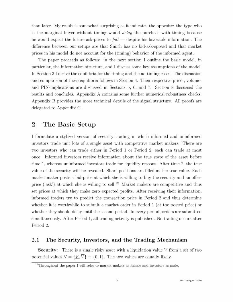
From the perspective of a trader, between today and tomorrow, one of three events
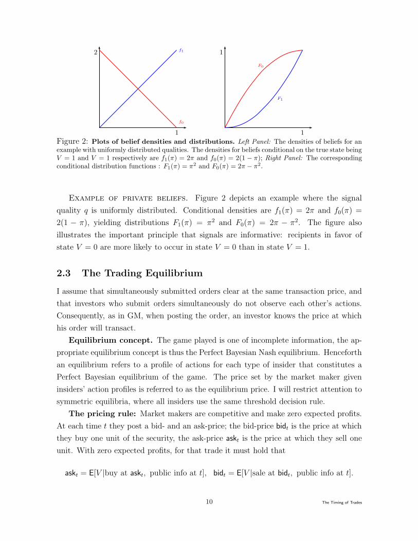
happens: the other trader either buys, or sells, or does not trade. Figure 3 illustrates
16 The Timing of Trades
t = 1 t = 2
ask1
E[V ]
bid1
ask2
E[V |buy]
bid2
t = 1 t = 2
ask1
E[V ]
bid1
ask2
E[V |sale]
bid2
t = 1 t = 2
ask1
E[V ]
bid1
ask2
E[V |hold]
bid2
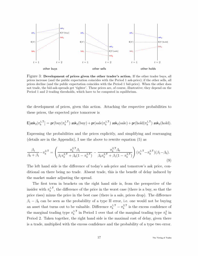
other buys other sells other holds
Figure 3: Development of prices given the other trader’s action. If the other trader buys, allprices increase (and the public expectation coincides with the Period 1 ask-price); if the other sells, allprices decline (and the public expectation coincides with the Period 1 bid-price). When the other doesnot trade, the bid-ask-spreads get ‘tighter’. These prices are, of course, illustrative; they depend on thePeriod 1 and 2 trading thresholds, which have to be computed in equilibrium.
the development of prices, given this action. Attaching the respective probabilities to
these prices, the expected price tomorrow is
E[ask2|π1,Tb ] = pr(buy|π1,T
b ) ask2(buy)+pr(sale|π1,Tb ) ask2(sale)+pr(hold|π1,T
b ) ask2(hold).
Expressing the probabilities and the prices explicitly, and simplifying and rearranging
(details are in the Appendix), I use the above to rewrite equation (5) as
β1
β0 + β1
−π2,Tb =
(
π2,Tb β1
β1π2,Tb + β0(1 − π2,T
b )−
π2,Tb β0
β0π2,Tb + β1(1 − π2,T
b )
)
(π1,Tb −π2,T
b )(β1−β0).
(9)
The left hand side is the difference of today’s ask-price and tomorrow’s ask price, con-
ditional on there being no trade. Absent trade, this is the benefit of delay induced by
the market maker adjusting the spread.
The first term in brackets on the right hand side is, from the perspective of the
insider with π1,Tb , the difference of the price in the worst case (there is a buy, so that the
price rises) minus the price in the best case (there is a sale, prices drop). The difference
β1 − β0 can be seen as the probability of a type II error, i.e. one would not be buying
an asset that turns out to be valuable. Difference π1,Tb − π2,T
b is the excess confidence of
the marginal trading type π1,Tb in Period 1 over that of the marginal trading type π2
b in
Period 2. Taken together, the right hand side is the maximal cost of delay, given there
is a trade, multiplied with the excess confidence and the probability of a type two error.
17 The Timing of Trades
The equation for sales is analogous.
Theorem 3 (Existence of the Period 1 Timing Thresholds)
There exist thresholds π1,Tb , π1,T
s that solve (9) and π1,Tb = 1 − π1,T
s .
To prove this theorem one needs to show that there exists a solution to equation (9).
The proof then first argues that when setting π1,Tb ≡ π1,M
b , then the left hand side of (9)
is larger than the right hand side. Likewise, when π1,Tb ≡ 1, then the right hand side is
larger than the left hand side (it is 0, the LHS is negative). Since both the left and the
right hand sides are continuous functions of π1,Tb , a solution exists.
4 Comparison of Marginal Trading Types
To compare the marginal trading types I will first derive two useful properties of the
second period thresholds. First, the buy-threshold maximizes the ask price24 and second,
the Period 2 buy-threshold is an increasing function of the Period 1 buying threshold.
Together these results are used to show that the timing buy-thresholds are always larger
than the myopic ones; by analogy the opposite holds for the sell-threshold.
Proposition 1 (Thresholds maximize the Bid-Ask-Spread)
The Period 2 ask-price as a function of the marginal buying type is maximized at the
equilibrium buying threshold π2
b . The same holds for the myopic Period 1 ask-price which
is maximized by the equilibrium buy-threshold π1,Mb .
The above result is quite intuitive: The ask price is set so that it averages signal qual-
ities over a range. The trader who is indifferent between trading and abstaining is the
marginal buying trader. So intuitively, in equilibrium the average quality (plus noise)
must coincide with the marginal quality; and as in many economic problems this occurs
when the average (i.e. the ask price as a function of the marginal trader’s belief) is
maximal.
Proposition 2 (Period 2 Bid-Ask-Spread Increases in Period 1 Thresholds)
The second period ask-price ask2 increases in the first-period buying threshold; the second
period bid-price bid2 decreases in the first-period selling threshold.
24This result is similar to one in Herrera and Smith (2006) who derive it in a different context; theydo not use it to study trade-timing. They kindly allowed me to study their private notes; I attempted aproof for my setting after I observed their result and I do not claim novelty; the proof techniques differ.The intuition for their result and mine coincides.
18 The Timing of Trades
This proposition implies that the larger the fraction of informed traders who delay in
Period 1, the larger the bid-ask-spread in Period 2; this result is irrespective of whether
or not behavior is myopic.
I will now proceed to compare the marginal trading types and I will focus on the
buy-side of the market. The marginal myopic buying threshold types in Period 1 and 2
are labeled π1,Mb , π2,M
b , the timing ones π1,Tb , π2,T
b .
Proposition 3 (Timing Marginal Trading Types are Larger)
Compared to the myopic scenario, with timing,
(a) the Period 1 buying-threshold is larger, π1,Tb ≥ π1,M
b ,
(b) the Period 2 buying-threshold is larger, π2,Tb ≥ π2,M
b .
To see the first point, observe that when employing threshold π1,Mb in expression (9), the
left hand side of (9) becomes π1,Mb − π2,T
b . In the Proof of Theorem 3 I then argue that
π1,Mb − π2,T
b >
(
π2,Tb β1
β1π2,Tb + β0(1 − π2,T
b )−
π2,Tb β0
β0π2,Tb + β1(1 − π2,T
b )
)
(β1 − β0)(π1,Mb − π2,T
b ).
To see the inequality indeed goes this way, observe that the term π1,Mb −π2,T
b cancels, and
the first and second terms on the right hand side are smaller than 1; so the direction of
the inequality is true. Applying the same interpretation as before, the price advantage of
delay (the left hand side) is larger than the cost (measured by the worst case-best case
price difference multiplied with the probability of a type-II error, adjusted for excess
confidence). This implies that when taking the delay option into account, the marginal
myopic buying type strictly prefers to delay.
Part (b) follows immediately from Proposition 2.
5 Bid-Ask Spreads and Price Variability
A major objective of Glosten-Milgrom type sequential trading models is to understand
the role and the size of bid-ask-spreads, askt − bidt. As the above analysis indicates, the
equilibrium buying threshold with timing is always larger than without timing. At first
sight, it appears that this should lead to larger bid-ask-spreads, because market makers
are now dealing with informed traders that on average have better information than in
a myopic equilibrium. Trading with people who have better information is costly, and
so to defend themselves, one might think, market makers need to increase the spread.
It turns out, that this intuition is incomplete.
19 The Timing of Trades
marginalmyopic
buyer
marginaltimingbuyer
myopic ask1
timing ask1
private expectation|signal&quality
ask1|marginal quality
signalquality Period 1 Period 2
ask1
bid1
ask2
bid2
Period 1 Period 2
ask1
bid1
ask2
bid2
ask price with timing vs. myopic myopic prices in Periods 1 and 2 timing prices in Periods 1 and 2
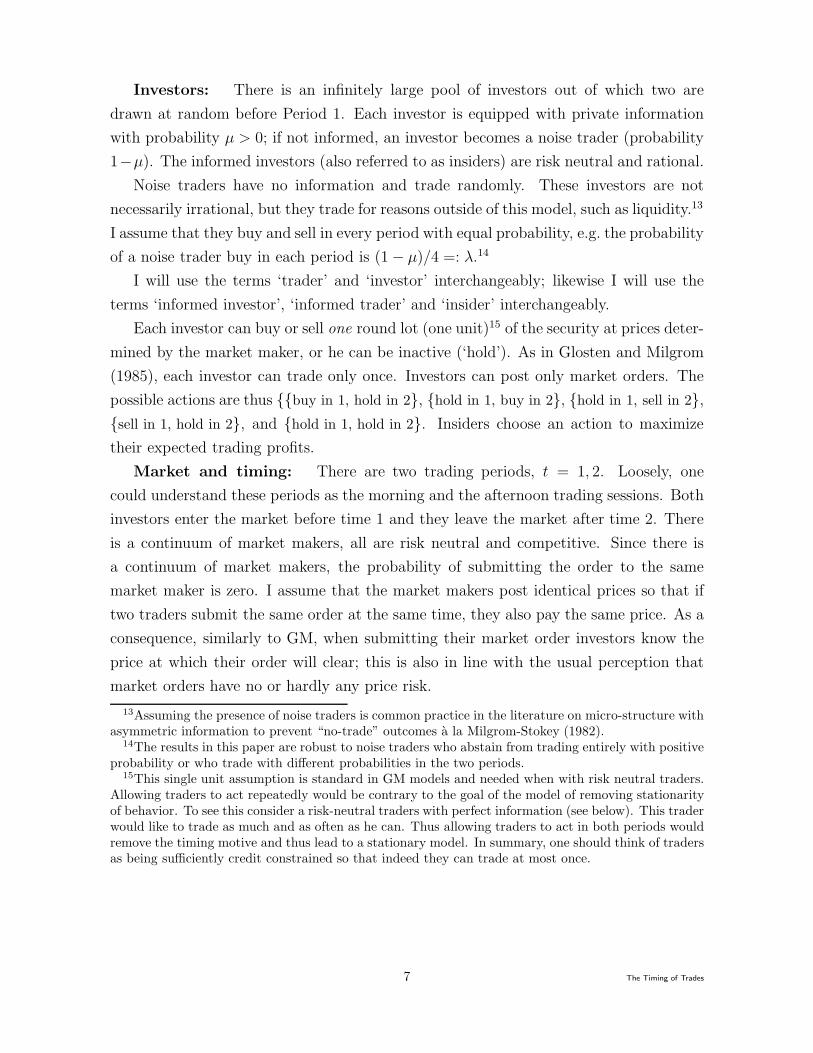
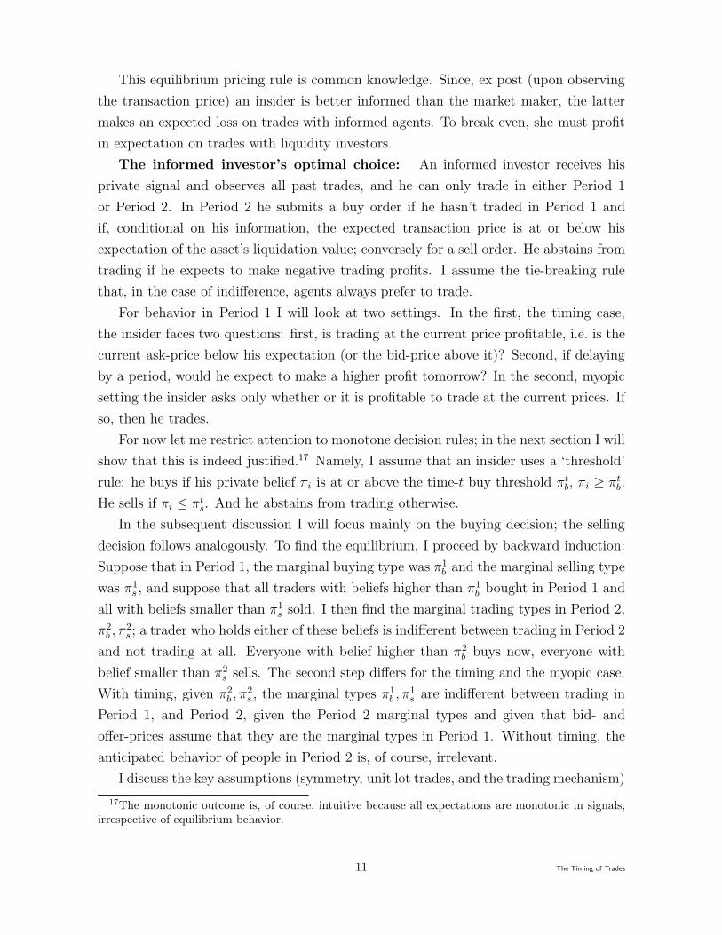
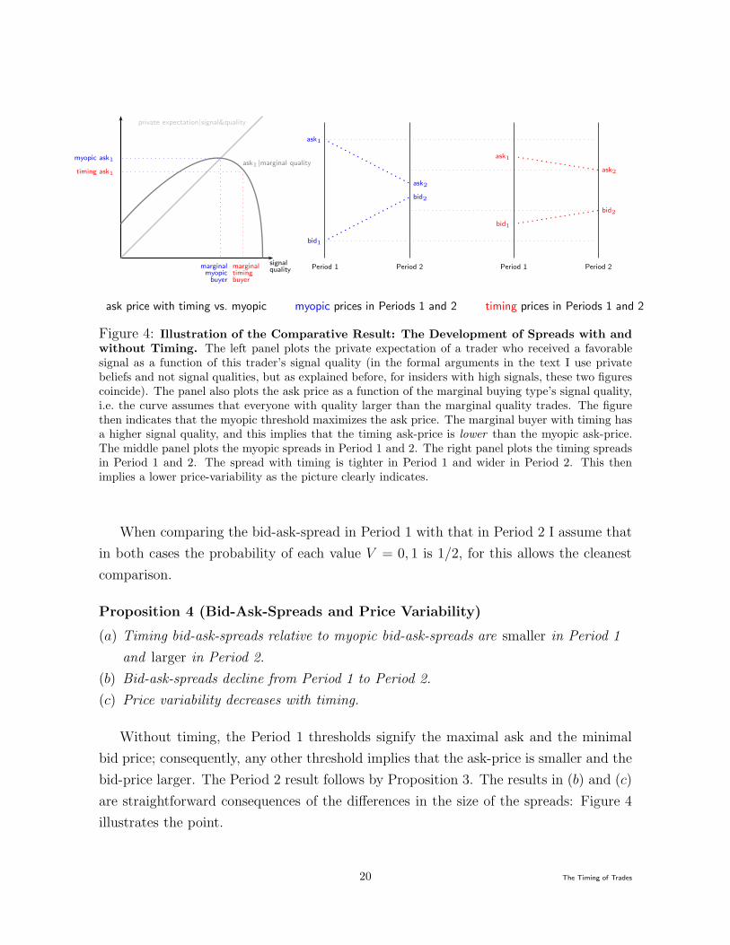
Figure 4: Illustration of the Comparative Result: The Development of Spreads with and
without Timing. The left panel plots the private expectation of a trader who received a favorablesignal as a function of this trader’s signal quality (in the formal arguments in the text I use privatebeliefs and not signal qualities, but as explained before, for insiders with high signals, these two figurescoincide). The panel also plots the ask price as a function of the marginal buying type’s signal quality,i.e. the curve assumes that everyone with quality larger than the marginal quality trades. The figurethen indicates that the myopic threshold maximizes the ask price. The marginal buyer with timing hasa higher signal quality, and this implies that the timing ask-price is lower than the myopic ask-price.The middle panel plots the myopic spreads in Period 1 and 2. The right panel plots the timing spreadsin Period 1 and 2. The spread with timing is tighter in Period 1 and wider in Period 2. This thenimplies a lower price-variability as the picture clearly indicates.
When comparing the bid-ask-spread in Period 1 with that in Period 2 I assume that
in both cases the probability of each value V = 0, 1 is 1/2, for this allows the cleanest
comparison.
Proposition 4 (Bid-Ask-Spreads and Price Variability)
(a) Timing bid-ask-spreads relative to myopic bid-ask-spreads are smaller in Period 1
and larger in Period 2.
(b) Bid-ask-spreads decline from Period 1 to Period 2.
(c) Price variability decreases with timing.
Without timing, the Period 1 thresholds signify the maximal ask and the minimal
bid price; consequently, any other threshold implies that the ask-price is smaller and the
bid-price larger. The Period 2 result follows by Proposition 3. The results in (b) and (c)
are straightforward consequences of the differences in the size of the spreads: Figure 4
illustrates the point.
20 The Timing of Trades
Proposition 4 outlines the dynamic behavior of the bid-ask spread: myopic spreads
are larger early on and smaller later-on than timing spreads. With timing the market
maker sets a spread that makes one type (π1,Tb ) indifferent between trading in Period 1
and 2. Thus with timing spreads should not vary dramatically between periods.
The following observations are based on numerical computations for the quality dis-
tribution in expressions (1) and (2) confirm this intuition.
Numerical Observation 1 (Spreads) Without timing the change in the size of the
spreads is larger than with timing.
Figure 5 plots these Period 1 and Period 2 spreads for both the myopic (right panels)
and the timing case (left panels). The top row plots spreads for the quadratic quality
the feasible parameter space for θ; the middle row for hill-shaped Beta quality (θ ≥ 1);
and the bottom row for U-shaped Beta-quality (θ < 1). With the quadratic quality
distribution, the timing spreads are almost identical for both periods. With the Beta
distribution timing spreads are not as similar across period as with the quadratic dis-
tribution, but the change in timing-spreads between periods is still much smaller than
with myopic-spreads.
Bid-ask spreads are the most basic form of transaction costs. Their size typically
depends on market liquidity — the more liquid the market, the smaller the spread.
Thus empirically one usually measures liquidity by the size of bid-ask-spreads.25 Ceteris
paribus, a smaller spread indicates that there is an absolute increase in liquidity trading.
The above result highlights a second feature: changes in the size of the bid-ask spread
can also account for a change in the relative importance of liquidity trading, i.e. in
the ratio of informed to uninformed trading. While with timing, ‘early’ on the average
quality of informed trading is larger than in the myopic case, the probability that the
market maker actually encounters such an informed trader is smaller.
6 The Dynamics of Volume
With two players a natural proxy for (average) volume is the probability that a given
market participant trades, i.e. the probability of a buy plus the probability of a sale.
Since the model is symmetric, this is, of course, the same as Vt = βt1+βt
0, where in abuse
of notation I shall use β2
i = λ + µ(Fi(π1
b ) − Fi(π2
b )). I can then show:
25Aitken and Comerton-Forde (2003) contains an extensive literature review on measures of liquidity.
21 The Timing of Trades
Proposition 5 (Total Volume) Compared to the myopic scenario, with timing,
(a) Period 1 volume is lower and
(b) total average volume measured across both periods is lower.
This follows because total volume depends on the fraction of informed investors who
trade and if thresholds are more extreme, as is the case with timing, then volume is
smaller.
To understand intraday volume patterns it is useful to understand how volume
changes from Period 1 to Period 2. Simplifying and rearranging it is straightforward
to see that
V1 − V2 has the same sign as 1 − G(π1
b ) − (G(π1
b ) − G(πb2)). (10)
In other words, the difference of volume in Period 1 and 2 is proportional to the difference
of the probability that an informed investor trades in Period 1 or 2. For instance, when
quality is uniformly distributed, the change in volume between periods from (10) depends
on the sign of (1+π2
b )/2−π1
b . Consequently, volume in Period 1 is larger than in Period
2 if and only if the average belief of all people who trade exceeds the marginal belief of
people trading in Period 1.
The bid-ask-spread in each period is proportional to the average signal quality of
trading agents multiplied with the probability that traders with this signal quality are
actually present, since
β1
1= λ+µ · (1−F1(π
1
b )) has the same sign as
∫
1
π1b
q · g(q) dq = (1−G(π1
b )) E[q|q ≥ π1
b ].
With timing, the market maker sets prices to ensure that the spread does not change
dramatically between periods. Since the average signal quality between Period 1 and 2
must decline, the probability of someone trading must increase in Period 2 relative to
Period 1. As a consequence, volume increases in from Period 1 to Period 2.
In the myopic case, on the other hand, the spread intuitively screens out a, loosely,
equally large proportion of the remaining quality types in every period. Since there is
simply a larger fraction of types in Period 1 than in Period 2, volume will be decreasing
from Period 1 to Period 2.
Numerical Observation 2 (Early vs. Late Volume) In the myopic case volume de-
creases from Period 1 to 2, whereas with timing volume rises from Period 1 to 2.
22 The Timing of Trades
Figure 6 has six panels: the left panels plot the Period 1 and Period 2 volume
proxy for the timing case, the right panels plot the Period 1 and Period 2 volume for
the myopic case. The top row uses the quadratic quality distribution from (1) over
the feasible parameter space for θ, with the level of insider trading µ ∈ [0.1, 0.9]; the
middle row plots volumes for the beta-distribution from (2) for parameter θ ∈ [1, 10]
and µ ∈ [.25, .75];26 and the bottom row plots volume for beta-distribution from (2) for
parameter θ ∈ [1/10, 1] and µ ∈ [.25, .75]. In all cases, with timing the Period 1 volume
is smaller than the Period 2 volume, and the reverse holds without timing.
Empirically, the pattern of volume differs across markets. For NYSE and Nasdaq
volume is usually said to be U- or reverse J-shaped.27 On London Stock Exchange,
on the other hand, recent evidence shows that volume is reverse L-shaped, with two
small humps, one in the morning and the other in the early afternoon.28 Other world
markets, for instance, the Taiwan and the Singapore Stock exchanges have reverse L-
shaped volume/number of transactions.29 Spreads are L-shaped on most markets.30
The patterns of volume and spreads that my model predicts would intuitively remain
consistent even if there would be more periods or more traders, i.e. myopic spreads would
fall stronger than timing spreads and volume would be increasing with and decreasing
without timing. So since my formulation predicts monotonic volume and thus cannot
possibly capture U-shaped volume, what is it that it can say? First one should note that
public information that appears overnight is usually reflected in the behavior during the
opening sessions. Markets then react to the information revealed by the behavior in
the opening sessions and this leads to active behavior early in the day. This reaction
to the opening session is nicely documented by the behavior on the LSE where around
the opening of the North American exchanges on the East Coast there is a ‘hump’ of
activity. Most information that affects the opening session, however, is public, whereas
information that spreads throughout the trading day is probably private or at least
has a private component (otherwise, with public information, there would be a trading
halt). Arguably, my model is applicable to exactly these situations, where information
is obtained during the day and after the opening session.
26For smaller and larger µ the rounding error gets too large for the Beta distribution.27See, for instance, Jain and Joh (1988), Brock and Kleidon (1992), McInish and Wood (1992), Lee,
Mucklow, and Ready (1993), or Brooks, Hinich, and Patterson (2003), for Nasdaq see, for instance,Chan, Christie, and Schultz (1995).
28The classic reference is Kleidon and Werner (1996), the more recent one Cai, Hudson, and Keasey(2004).
29For Taiwan, see Lee, Fok, and Liu (2001); for Singapore see Ding and Lau (2001).30Earlier papers find that spreads are U-shaped on NYSE, but recent evidence (Serednyakov (2005))
suggests that the pattern of spreads has morphed to an L-shape after decimalization.
23 The Timing of Trades
My analysis is thus consistent with the volume and spread declines that occur towards
the end of the trading day. Importantly my GM-model with timing displays these
patterns without having to assume that certain types of traders exogenously cluster at
specific times of the day. A GM model with timing thus reconciles that informed agents
would trade early, inducing an equilibrium separation of better and less-well informed
traders that leads to precisely the volume-spread-patterns that are observed on most
exchanges towards the end of the trading day. Since behavior in GM models is fully
rational, the volume-spreads patterns towards the end of the trading day should no
longer be considered surprising or puzzling.
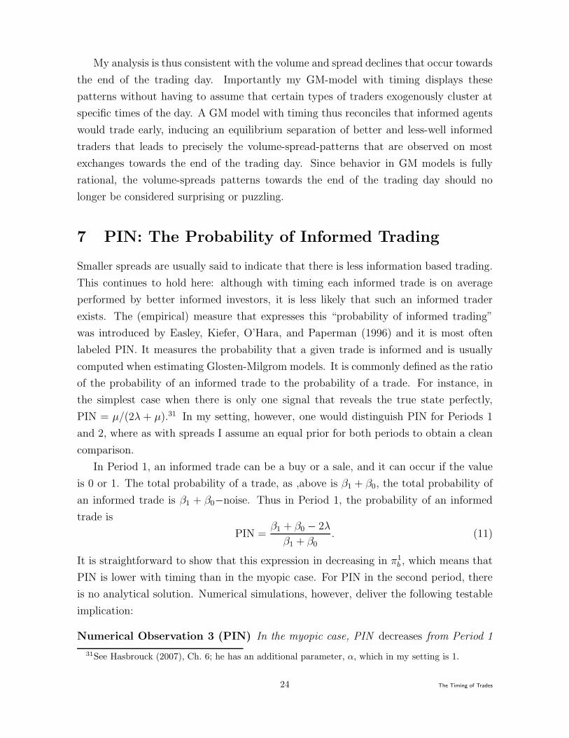
7 PIN: The Probability of Informed Trading
Smaller spreads are usually said to indicate that there is less information based trading.
This continues to hold here: although with timing each informed trade is on average
performed by better informed investors, it is less likely that such an informed trader
exists. The (empirical) measure that expresses this “probability of informed trading”
was introduced by Easley, Kiefer, O’Hara, and Paperman (1996) and it is most often
labeled PIN. It measures the probability that a given trade is informed and is usually
computed when estimating Glosten-Milgrom models. It is commonly defined as the ratio
of the probability of an informed trade to the probability of a trade. For instance, in
the simplest case when there is only one signal that reveals the true state perfectly,
PIN = µ/(2λ + µ).31 In my setting, however, one would distinguish PIN for Periods 1
and 2, where as with spreads I assume an equal prior for both periods to obtain a clean
comparison.
In Period 1, an informed trade can be a buy or a sale, and it can occur if the value
is 0 or 1. The total probability of a trade, as ,above is β1 + β0, the total probability of
an informed trade is β1 + β0−noise. Thus in Period 1, the probability of an informed
trade is
PIN =β1 + β0 − 2λ
β1 + β0
. (11)
It is straightforward to show that this expression in decreasing in π1
b , which means that
PIN is lower with timing than in the myopic case. For PIN in the second period, there
is no analytical solution. Numerical simulations, however, deliver the following testable
implication:
Numerical Observation 3 (PIN) In the myopic case, PIN decreases from Period 1
31See Hasbrouck (2007), Ch. 6; he has an additional parameter, α, which in my setting is 1.
24 The Timing of Trades
to Period 2; with timing, PIN increases from Period 1 to 2.
Figure 5 plots PIN for Period 1 and Period 2 for both the myopic (right panels) and
the timing case (left panels). The top row plots PIN for the quadratic quality over the
feasible parameter space for θ; the middle row plots PIN for the hill-shaped Beta quality
(θ ≥ 1); and the bottom row plots PIN for the U-shaped Beta-quality (θ < 1).
One could loosely interpret the first period in my setting as the morning session, and
the second period as the afternoon session. If timing does occur as outlined in my model,
then PIN should be higher in the afternoon than in the morning — despite the fact the
better informed traders move in the morning. With myopic trading, the situation is
reversed.
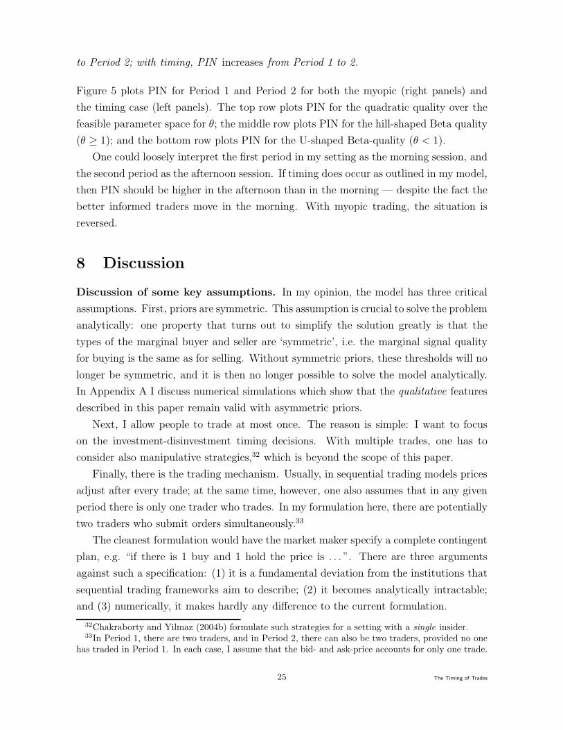
8 Discussion
Discussion of some key assumptions. In my opinion, the model has three critical
assumptions. First, priors are symmetric. This assumption is crucial to solve the problem
analytically: one property that turns out to simplify the solution greatly is that the
types of the marginal buyer and seller are ‘symmetric’, i.e. the marginal signal quality
for buying is the same as for selling. Without symmetric priors, these thresholds will no
longer be symmetric, and it is then no longer possible to solve the model analytically.
In Appendix A I discuss numerical simulations which show that the qualitative features
described in this paper remain valid with asymmetric priors.
Next, I allow people to trade at most once. The reason is simple: I want to focus
on the investment-disinvestment timing decisions. With multiple trades, one has to
consider also manipulative strategies,32 which is beyond the scope of this paper.
Finally, there is the trading mechanism. Usually, in sequential trading models prices
adjust after every trade; at the same time, however, one also assumes that in any given
period there is only one trader who trades. In my formulation here, there are potentially
two traders who submit orders simultaneously.33
The cleanest formulation would have the market maker specify a complete contingent
plan, e.g. “if there is 1 buy and 1 hold the price is . . . ”. There are three arguments
against such a specification: (1) it is a fundamental deviation from the institutions that
sequential trading frameworks aim to describe; (2) it becomes analytically intractable;
and (3) numerically, it makes hardly any difference to the current formulation.
32Chakraborty and Yilmaz (2004b) formulate such strategies for a setting with a single insider.33In Period 1, there are two traders, and in Period 2, there can also be two traders, provided no one
has traded in Period 1. In each case, I assume that the bid- and ask-price accounts for only one trade.
25 The Timing of Trades

To elaborate, GM frameworks are the purest formulations of quote-driven markets;
a complete contingent plan, however, more closely resembles a market which is usually
described as order-driven. Moreover, in such an order-driven market, it would no longer
be possible to describe a meaningful bid-ask-spread, because there would be no unique
quotes for bid- and ask-prices.34 Traders also would not know at which price their market
orders clear, and so such a setting would rather resemble a batch auction.
The complete-contingent plan setting is also analytically far less tractable: first,
since traders do not know at which price their order will clear, they have to compute
their expectation of the Period 1 transaction price. Next, when computing the Period 2
expected (ask- or bid-) price, if there is a hold, then, again, in Period 2 one has to
compute the expected transaction price. Conceptually, this is not a problem, but there
is no analytical solution. Finally, comparing numerical simulations of the complete-
contingent price-plan with single-price settings, it turns out that the numerical difference
in the thresholds is minor.
Another way to think about the formulation that I propose is to suppose that market
makers first post their limit orders (i.e. their bid and offer prices) simultaneously and that
in doing so, several will post identical orders, so that there will be standing limit orders at
identical prices.35 With a fast electronic trade-through system, simultaneously submitted
orders would then be cleared so quickly that the limit orders cannot be adjusted.
The purpose of this study is to understand the timing decision of informed traders
who potentially face ‘informational’ competition. I choose the simplest possible for-
mulation that allows insights into this problem. The key element is the anticipated
information content of present and future trades and its impact on prices. The results
do not hinge on the assumptions of symmetry or a single price for simultaneous orders.
What would happen if there are ‘strategic’ noise traders? Suppose some
fraction of the 1 − µ noise traders can choose when to trade. Such people would be
uninformed traders who have to trade for liquidity reasons but who can choose when to
trade. So when would they? Let me start with making an out-of-equilibrium observation:
Having no information is equivalent to receiving a signal of quality 1/2; the corresponding
belief is π = 1/2. By monotonicity, traders with belief below π1
b delay in Period 1 because
they believe that ‘things will get better’ in Period 2. Thus delaying is a dominant strategy
34In particular, there would be a price for ‘matched’ trades, i.e. when the number of simultaneousbuys and sales coincide.
35This is commonly observed; Level 2 views of the Market Book offered by stock exchanges (e.g. theTSX) usually provide views based on orders (“market-by-order”) and price (“market-by-price”). Thelatter view aggregates all limit orders for identical prices, and usually there are multiple orders for suchprices.
26 The Timing of Trades

for this uninformed (liquidity) trader. If there are strategic delays of noise traders then
there would an equilibrium effect on the marginal trading types. The reason is that
when the fraction of noise traders who act in Period 1 declines, ceteris paribus, then
spreads widen. By the same token, when there are more noise traders in Period 2, then
the spread tighten. Yet despite these two effects, in equilibrium spreads must still shrink
between periods because of the belief monotonicity. As a consequence, strategic noise
traders would always trade in Period 2.
Discussion of the Results. In ‘classic’ models of sequential trade, agents cannot
choose the time of market entry. In such models private and public beliefs converge,
thus the bid-ask spread gets smaller. While in my model spreads also decrease between
periods, the trajectory with timing is flatter (with the reservation that, obviously, a two
period model is not fit to project limit arguments).
Furthermore, as Smith (2000) points out, an investor with a favorable signal expects
transaction prices to increase (for him it is a sub-martingale). Casual intuition then
suggests, that profits from speculation are largest early – thus investors should invest
rather earlier than later. My result is somewhat surprising as it indicates the opposite:
the type who is the marginal buyer without timing would delay the purchase with timing
because he would expect future ask-prices to fall — despite his favorable information.
My model is, of course, very restrictive; in real markets, it is quite possible that there
are combinations of myopic and timing behavior. For instance, the large volume at and
just after the open may result from traders who act on new information that arrived
during the night, and these traders may act myopically. At the same time, the volume
upswing towards the close could be forced by strategic timers who receive information
during the day. The restriction to two periods and two traders, however, is not a strong
one: the intuition for behavior would carry through to settings with more trading periods
and more traders.
A Appendix: Numerical Robustness
with Asymmetric Priors
The numerical computations presented in this appendix employ the example from Sec-
tion 2 with signal densities f1(π) = 2π, f0(π) = 2(1 − π) as plotted in Figure 2. Recall
that these distributions together lead to an ex-ante uniform distribution of beliefs.
Asymmetric Priors. For the main results of this paper I have assumed an equal
prior for the liquidation values V . I did this, because it simplifies the exposition and
allows analytical results. Moreover, the prior actually does affect the computation of
27 The Timing of Trades
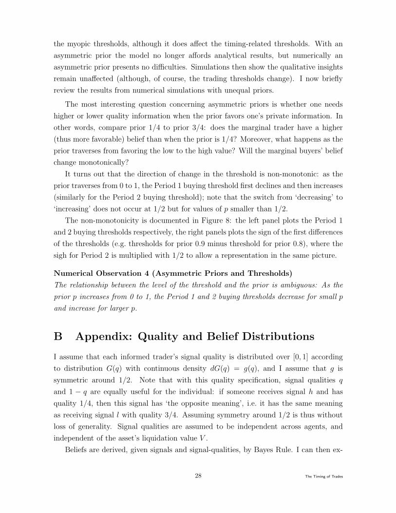
the myopic thresholds, although it does affect the timing-related thresholds. With an
asymmetric prior the model no longer affords analytical results, but numerically an
asymmetric prior presents no difficulties. Simulations then show the qualitative insights
remain unaffected (although, of course, the trading thresholds change). I now briefly
review the results from numerical simulations with unequal priors.
The most interesting question concerning asymmetric priors is whether one needs
higher or lower quality information when the prior favors one’s private information. In
other words, compare prior 1/4 to prior 3/4: does the marginal trader have a higher
(thus more favorable) belief than when the prior is 1/4? Moreover, what happens as the
prior traverses from favoring the low to the high value? Will the marginal buyers’ belief
change monotonically?
It turns out that the direction of change in the threshold is non-monotonic: as the
prior traverses from 0 to 1, the Period 1 buying threshold first declines and then increases
(similarly for the Period 2 buying threshold); note that the switch from ‘decreasing’ to
‘increasing’ does not occur at 1/2 but for values of p smaller than 1/2.
The non-monotonicity is documented in Figure 8: the left panel plots the Period 1
and 2 buying thresholds respectively, the right panels plots the sign of the first differences
of the thresholds (e.g. thresholds for prior 0.9 minus threshold for prior 0.8), where the
sigh for Period 2 is multiplied with 1/2 to allow a representation in the same picture.
Numerical Observation 4 (Asymmetric Priors and Thresholds)
The relationship between the level of the threshold and the prior is ambiguous: As the
prior p increases from 0 to 1, the Period 1 and 2 buying thresholds decrease for small p
and increase for larger p.
B Appendix: Quality and Belief Distributions
I assume that each informed trader’s signal quality is distributed over [0, 1] according
to distribution G(q) with continuous density dG(q) = g(q), and I assume that g is
symmetric around 1/2. Note that with this quality specification, signal qualities q
and 1 − q are equally useful for the individual: if someone receives signal h and has
quality 1/4, then this signal has ‘the opposite meaning’, i.e. it has the same meaning
as receiving signal l with quality 3/4. Assuming symmetry around 1/2 is thus without
loss of generality. Signal qualities are assumed to be independent across agents, and
independent of the asset’s liquidation value V .
Beliefs are derived, given signals and signal-qualities, by Bayes Rule. I can then ex-
28 The Timing of Trades

press the belief densities as follows: in state V = 1, the generalized density of individuals
with private belief π is f1(π) = π[dG(π) + dG(1 − π)], while analogously, in the ‘low’
state, V = 0, it is f0(π) = (1 − π)[dG(π) + dG(1 − π)].
Smith and Sørensen (2000) prove the following property of private beliefs:
Lemma 1 (Symmetric beliefs, Smith and Sørensen (2000))
With the above the signal quality structure, private belief distributions satisfy F1(π) =
1 − F0(1 − π) for all π ∈ (0, 1).
The signal densities satisfy the monotone likelihood ratio property. This is straight-
forward to see because the likelihood ratio, expressed through the ratio of the belief
densities,f1(π)
f0(π)=
π[dG(π) + dG(1 − π)]
(1 − π)[dG(π) + dG(1 − π)]=
π
1 − π
is increasing in π.
C Omitted Proofs
Proof of Theorem 1 (Existence, Uniqueness, and Symmetry)
We have already argued the symmetry of Period 2 thresholds, monotonicity of trading
rules and informativeness of trades. I have shown that the Period 2 threshold, π2
b , is
π2
b =β2
1
β2
1+ β2
0
⇔ π2
b =λ + µ(F1(π
1
b ) − F1(π2
b ))
λ + µ(F1(π1
b ) − F1(π2
b )) + λ + µ(F0(π1
b ) − F0(π2
b )). (12)
Trade informativeness immediately implies that π2
b must be at least 1/2. What
remains to show is existence and uniqueness of π2
b ∈ [1/2, π1
b ).
From equation (12) we know that the threshold quality for buying depends on the
relative probability of high correct to high wrong beliefs. We will now reformulate (12)
to obtain a more manageable relation: First,
F1(π) =
∫ π
0
f1(s) ds =
∫ π
0
s · (g(s) + g(1 − s)) ds = 2
∫ π
0
s · g(s) ds,
where the last step follows from the symmetry of g around 1/2. Performing integration
by parts, we obtain
F1(π) = 2
∫ π
0
s · g(s) ds = 2sG(s)|π0− 2
∫ π
0
G(s) ds = 2πG(π) − 2
∫ π
0
G(s) ds.
29 The Timing of Trades
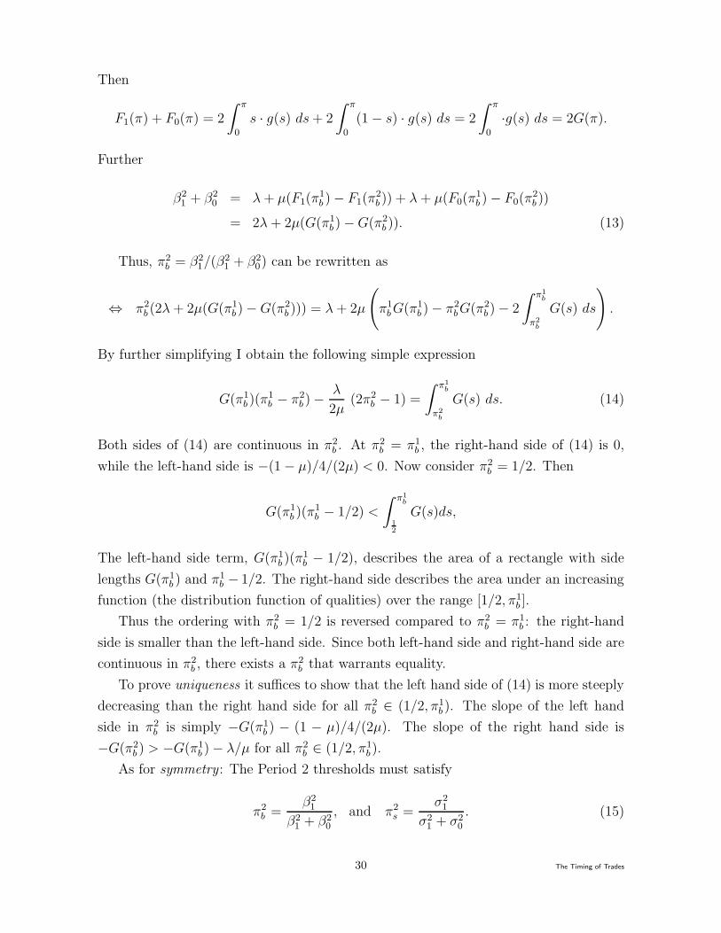
Then
F1(π) + F0(π) = 2
∫ π
0
s · g(s) ds + 2
∫ π
0
(1 − s) · g(s) ds = 2
∫ π
0
·g(s) ds = 2G(π).
Further
β2
1+ β2
0= λ + µ(F1(π
1
b ) − F1(π2
b )) + λ + µ(F0(π1
b ) − F0(π2
b ))
= 2λ + 2µ(G(π1
b ) − G(π2
b )). (13)
Thus, π2
b = β2
1/(β2
1+ β2
0) can be rewritten as
⇔ π2
b (2λ + 2µ(G(π1
b ) − G(π2
b ))) = λ + 2µ
(
π1
bG(π1
b ) − π2
bG(π2
b ) − 2
∫ π1b
π2b
G(s) ds
)
.
By further simplifying I obtain the following simple expression
G(π1
b )(π1
b − π2
b ) −λ
2µ(2π2
b − 1) =
∫ π1b
π2b
G(s) ds. (14)
Both sides of (14) are continuous in π2
b . At π2
b = π1
b , the right-hand side of (14) is 0,
while the left-hand side is −(1 − µ)/4/(2µ) < 0. Now consider π2
b = 1/2. Then
G(π1
b )(π1
b − 1/2) <
∫ π1b
12
G(s)ds,
The left-hand side term, G(π1
b )(π1
b − 1/2), describes the area of a rectangle with side
lengths G(π1
b ) and π1
b − 1/2. The right-hand side describes the area under an increasing
function (the distribution function of qualities) over the range [1/2, π1
b ].
Thus the ordering with π2
b = 1/2 is reversed compared to π2
b = π1
b : the right-hand
side is smaller than the left-hand side. Since both left-hand side and right-hand side are
continuous in π2
b , there exists a π2
b that warrants equality.
To prove uniqueness it suffices to show that the left hand side of (14) is more steeply
decreasing than the right hand side for all π2
b ∈ (1/2, π1
b ). The slope of the left hand
side in π2
b is simply −G(π1
b ) − (1 − µ)/4/(2µ). The slope of the right hand side is
−G(π2
b ) > −G(π1
b ) − λ/µ for all π2
b ∈ (1/2, π1
b ).
As for symmetry : The Period 2 thresholds must satisfy
π2
b =β2
1
β2
1+ β2
0
, and π2
s =σ2
1
σ2
1+ σ2
0
. (15)
30 The Timing of Trades

The probabilities of trades are computed as follows: Suppose for now that monotonicity
of decisions holds and let πb, πs denote the threshold values so that traders in Period
2 with private beliefs above πb buy and those with private beliefs below πs sell if they
have not traded in Period 1. Then
β2
i =λ + µ(Fi(π
1
b ) − Fi(πb))
γ1
i
, σ2
i =λ + µ(Fi(πs) − Fi(π
1
s))
γ1
i
, γ1
i = 2λ+µ(Fi(π1
b )−Fi(π1
s)).
For now assume that symmetry holds in Period 1, i.e π1
b = 1−π1
s . The quality paradigm
thus yields
F1(π1
b ) = 1 − F0(1 − π1
b ) ⇔ F1(π1
b ) = 1 − F0(π1
s ).
Suppose that also symmetry in Period 2 prevails. Then this ensures consistency
1 − π2
b = 1 −β2
1
β2
1+ β2
0
=β2
0
β2
1+ β2
0
=λ + µ(F0(π
1
b ) − F0(π2
b ))
λ + µ(F1(π1
b ) − F1(π2
b )) + λ + µ(F0(π1
b ) − F0(π2
b ))
=λ + µ(F1(π
2
s) − F1(π1
s))
λ + µ(F1(π2s) − F1(π1
s)) + λ + µ(F0(π2s) − F0(π1
s))=
σ2
1
σ2
1+ σ2
0
= π2
s .
Deriving Equation (9) from equation (5)
With symmetry I can express the probabilities for buys and sales in Period 1 by
β1
i = λ + µ(1 − Fi(π1
b )), σ1
i = λ + µFi(π1
s) = β1
|i−1|,
γ1
i = 2λ + µ(Fi(π1
b ) − Fi(π1
s)) = 1 − (β1
0+ β1
1).
The insider with belief π1
b then assigns the following probabilities to these events:
pr(buy|π1
b ) = π1
bβ1
1+ (1 − π1
b )β1
0, pr(sale|π1
b ) = π1
bβ1
0+ (1 − π1
b )β1
1,
pr(no trade|π1
b ) = 1 − (β1
1+ β1
0).
By symmetry γ1
1= γ1
0, so that the price in Period 2, given π1
b is found by solving the
following for π2
b .β2
1(π1
b , π2
b )
β2
1(π1
b , π2
b ) + β2
0(π1
b , π2
b )= π2
b .
As a consequence, I can expand each ask price in E[ask2|π1
b ] by substituting each β2
1in
Period 2’s price with the threshold π2
b and each β2
0with the threshold 1− π2
b . Omitting
superscripts t = 1 on βi,
ask2(buy) =β1π
2
b
β1π2
b + β0(1 − π2
b ), ask2(sale) =
β0π2
b
β0π2
b + β1(1 − π2
b ), ask2(hold) = π2
b .
31 The Timing of Trades
Since ask1 = β1/(β0 + β1), equation (5) expands to
β1
β1 + β0
=π1
bβ1 + (1 − π1
b )β0
β1π2
b + β0(1 − π2
b )β1π
2
b +π1
bβ0 + (1 − π1
b )β1
β0π2
b + β1(1 − π2
b )β0π
2
b + (1 − (β1 + β0))π2
b . (16)
One can rearrange and simplify this equation to yield equation (9)
⇔β1
β0 + β1
− π2
b =
(
π2
bβ1
β1π2
b + β0(1 − π2
b )−
π2
bβ0
β0π2
b + β1(1 − π2
b )
)
(π1
b − π2
b )(β1 − β0). (17)
Proof of Theorem 3 (Existence of Period 1 Timing Thresholds)
I focus only on the buy-threshold (the sale threshold argument is analogous) and I
proceed constructively: Suppose π1
b = 1. Then β1 = β0 and thus the LHS of (9) is
1/2 − π2
b ≤ 0 whereas the RHS is 0. Next, let π1
b = π1,Mb , where π1,M
b solves the myopic
problem. Then the LHS of (9) is π1
b − π2
b and we can reduce the LHS to 1 and the RHS,
using π1,Mb = β1/(β1 + β0) to
(
π2
bπ1
b
π1
bπ2
b + (1 − π1
b )(1 − π2
b )−
π2
b (1 − π1
b )
(1 − π1
b )π2
b + π1
b (1 − π2
b )
)
(β1 − β0). (18)
Naturally, both terms are smaller than 1 and thus the above expression is smaller than 1.
Since LHS and RHS of (9) are both continuous in π1
b , a solution exists.
Symmetry obtains straightforwardly: reformulate equation (16) for bid-prices, hy-
pothesizing a symmetric threshold. With a symmetric prior, pr(buy|π1
b ) = pr(sale|1−π1
b ),
ask1 = 1 − bid1 etc. Substituting this into (9) immediately yields the desired equality.
Proof of Proposition 1 (Equilibrium Threshold Beliefs Maximize the Spread)
Considering first order conditions, ∂∂π
E[V |Ht, buy with threshold π] = 0 is equivalent to
∂
∂π
β1(π)pt
β1(π)pt + β0(π)(1 − pt)= 0 ⇔
β0(π)
β1(π)=
β ′0(π)
β ′1(π)
. (19)
Now recall that β2
i (π) = (λ + µ(Fi(π1
b ) − Fi(π)))/γi. Thus the right hand side of the
second relation above isβ ′
0(π)
β ′1(π)
=f0(π)
f1(π).
In Appendix B I have argued that f1(π) = π[dG(π) + dG(1 − π)], and f0(π) =
32 The Timing of Trades
(1 − π)[dG(π) + dG(1 − π)]. With this we have
β ′0(π)
β ′1(π)
=1 − π
π. (20)
Next, consider the equilibrium condition Et[V |π] = ask2(π). Rearranging and simplify-
ing, threshold π must satisfyβ0(π)
β1(π)=
1 − π
π. (21)
Combining equations (19) and (20) delivers the same relation as equation (21) and thus
the equilibrium condition is identical to the First Order Condition for the ask price as a
function of threshold π.
Proof of Proposition 2 (Period 2 Spread increases in Period 1 Threshold)
The equilibrium condition for the Period 2 buying-threshold, equation (7), can be refor-
mulated to β1(π1
b , π2
b )/β0(π1
b , π2
b ) = π2
b/(1−π2
b ). To prove the statement of the proposition
it thus suffices to compute the derivative of β1(π1
b , π2
b )/β0(π1
b , π2
b ) with respect to π1
b and
show that it is positive:
∂
∂π1
b
β0(π1
b , π)
β1(π1
b , π)< 0 ⇔ f0(π
1
b )β2
1− f1(π
1
b )β2
0< 0 ⇔
f0(π1
b )
f1(π1
b )<
β2
0
β2
1
.
Using the above insights and the Period 2 equilibrium condition, this relation says that
(1 − π1
b )/π1
b < (1 − π2
b )/π2
b , which certainly holds as π1
b > π2
b .
Proof of Proposition 3 (Benchmark Comparison)
(a): To show π1,Tb > π1,M
b I will argue that π1,Tb 6≤ π1,M
b .
First, one can apply similar arguments as in Theorem 1 to show that π1,Mb is unique;
the proof for this is omitted. Next, recall that π1,Mb maximizes the ask-price. Also,
ask(1) = 1/2 whereas the private expectation for πb = 1 is 1. Consequently, it must hold
that for any π < π1,Mb , π < β1(π)/(β1(π) + β0(π)). So for every π < π1,M
b the left hand
side of (9) satisfiesβ1(π)
β1(π) + β0(π)− π2
b > π − π2
b .
By the same arguments as used in the proof of Theorem 3, the RHS of the above remains
larger than (
π2
bβ1
β1π2
b + β0(1 − π2
b )−
π2
bβ0
β0π2
b + β1(1 − π2
b )
)
(β1 − β0),
33 The Timing of Trades
because both terms in the latter are smaller than 1. Thus there cannot be a solution to
(9) for π < π1,Mb .
(b) follows immediately from (a) and Proposition 2.
(c) follows from (a) and (b) because higher thresholds imply that a smaller fraction
of informed agents trades.
Proof of Proposition 4 (Bid-Ask Spreads and Price Variability)
(a): The result follows from Propositions 1 and 3: without timing, the Period 1 thresholds
signify the maximal ask and the minimal bid price; consequently, any other threshold
implies that the ask-price is smaller and the bid-price larger.
With symmetry, the bid-ask spread in Period 2 with timing can be expressed by
threshold beliefs and it is thus π2,Tb − π2,T
s ; in the myopic case it is π2,Mb − π2,M
s . By
Proposition 3 (b), π2,Tb > π2,M
b and π2,Ts < π2,M
s .
(b): The result is immediately clear in the myopic case. In the timing case, observe
that the marginal buyer expects tomorrow’s ask price to be the same as today’s. Since
beliefs are monotonic, traders with higher beliefs consider tomorrow’s ask price to be
larger (because they consider buys more likely), and traders with beliefs lower than the
Period 1 buying threshold believe that prices will drop. In particular this holds for
traders with belief 1/2, which is the same as the public (unconditional) expectation.
Consequently, the ask price in Period 1 is unconditionally larger than the ask price in
Period 2; a symmetric result applies to the bid-prices. Thus the spread declines.
(c): Variability follows from the spread relation: with timing one moves from a smaller
to a larger spread. At the same time, the overall spread declines (in both cases), and
thus the change in prices is larger for the myopic case.
References
Abreu, D., and M. Brunnermeier (2003): “Bubbles and Crashes,” Econometrica,71(1), 173–204.
Admati, A., and P. Pfleiderer (1988): “A theory of intraday patterns: volume andprice variability,” Review of Financial Studies, 1, 3–40.
Aitken, M., and C. Comerton-Forde (2003): “How should liquidity be mea-sured?,” Pacific-Basin Finance Journal, 11(1), 45–50.
Avery, C., and P. Zemsky (1998): “Multi-Dimensional Uncertainty and Herd Be-havior in Financial Markets,” American Economic Review, 88, 724–748.
Back, K., and S. Baruch (2004): “Information in Securities Markets: Kyle meetsGlosten and Milgrom,” Econometrica, 72(2), 433–466.
34 The Timing of Trades
Brock, W., and A. Kleidon (1992): “Periodic Market Closure and Trading Volume— A Model of Intraday Bids and Asks,” Journal of Economic Dynamics and Control,16, 451–489.
Brooks, C., M. J. Hinich, and D. M. Patterson (2003): “Intraday Patterns inthe Returns, Bid-ask Spreads, and Trading Volume on Stocks Traded on the NewYork Stock Exchange,” Working paper, University of Reading.
Cai, C. X., R. Hudson, and K. Keasey (2004): “Intra Day Bid-Ask Spreads,Trading Volume and Volatility: Recent Empirical Evidence from the London StockExchange,” Journal of Business Finance and Accounting, 31(5), 647–676.
Chakraborty, A., and B. Yilmaz (2004a): “Informed Manipulation,” Journal ofEconomic Theory, 114(1), 132–152.
(2004b): “Manipulation in Market Order models,” Journal of Financial Mar-kets, 7, 187–206.
Chamley, C., and D. Gale (1994): “Information Revelation and Strategic Delay ina Model of Investment,” Econometrica, 62, 1065–1085.
Chan, K. C., W. G. Christie, and P. H. Schultz (1995): “Market Structureand the Intra-day Pattern of Bid-Ask Spreads for NASDAQ Securities,” Journal ofBusiness, 68(1), 35–60.
Chari, V., and P. J. Kehoe (2004): “Financial Crises as Herds: Overturning theCritiques,” Journal of Economic Theory, 119(1), 128–150.
Comerton-Forde, C., M. O’Brian, and P. J. Westerholm (2004): “An Empir-ical Analysis of Strategic Behavior Models,” Working paper, University of Sidney.
Ding, D. K., and S. T. Lau (2001): “An Analysis of Transactions Data for the StockExchange of Singapore: Patterns, Absolute Price Change, Trade Size and Number ofTransactions,” Journal of Business Finance and Accounting, 28(1), 151–174.
Easley, D., N. M. Kiefer, M. O’Hara, and J. B. Paperman (1996): “Liquidity,Information, and Infrequently Traded Stocks,” Journal of Finance, LI(4), 1405–1436.
Easley, D., and M. O’Hara (1987): “Price, Trade Size, and Information in SecuritiesMarkets,” Journal of Financial Economics, 19, 69–90.
Glosten, L., and P. Milgrom (1985): “Bid, Ask and Transaction Prices in a Special-ist Market with Heterogenously Informed Traders,” Journal of Financial Economics,14, 71–100.
Gul, F., and R. Lundholm (1995): “Endogenous Timing and Clustering of Agents’Decisions,” Journal of Political Economy, 103, 1039–1066.
Hasbrouck, J. (2007): Empirical Market Microstructure. Oxford University Press.
35 The Timing of Trades
Herrera, H., and L. Smith (2006): “private notes,” , University of Michigan.
Jain, P., and G. Joh (1988): “The Dependence of Hourly Prices and Trading Volume,”Journal of Financial and Quantitative Analysis, 23(3), 269–284.
Kleidon, A., and I. Werner (1996): “U.K. and U.S. trading of British cross-listedstocks: an intraday analysis of market integration,” Review of Financial Studies, 9,619–664.
Kyle, A. (1985): “Continuous Auctions and Insider Trading,” Econometrica, 53, 1315–1336.
Lee, C., B. Mucklow, and M. Ready (1993): “Spreads, Depth and the Impactof Earnings Information: An Intraday Analysis,” Review of Financial Studies, 6(2),345–374.
Lee, I. H. (1998): “Market Crashes and Informational Avalanches,” Review of Eco-nomic Studies, 65(4), 741–759.
Lee, Y.-T., R. C. Fok, and Y.-J. Liu (2001): “Explaining Intraday Pattern of Trad-ing Volume From Order Flow Data,” Journal of Business Finance and Accounting,28(1), 199–230.
Lin, J., G. Sanger, and G. Booth (1995): “Trade Size Components of the bid-ask-spread,” Review of Financial Studies, 8, 1153–1183.
Madhavan, A., M. Richardson, and M. Roomans (1997): “Why do security priceschange? A transaction-level analysis of NYSE stocks,” Review of Financial Studies,10, 1035–1064.
Malinova, K., and A. Park (2008): “Continuous Trading vs. Batch Auctions,” mi-neo, University of Toronto.
McInish, T., and R. Wood (1992): “An Analysis of Intraday Patterns in Bid-AskSpreads for NYSE Stocks,” Journal of Finance, 47(2), 753–764.
Serednyakov, A. (2005): “A Model of the Components of the Bid-Ask Spread,”Working paper, University of Minnesota.
Smith, L. (2000): “Private Information and Trade Timing,” American Economic Re-view, 90, 1012–1018.
Smith, L., and P. Sørensen (2000): “Pathological Outcomes of Observational Learn-ing,” Econometrica, 68, 371–398.
36 The Timing of Trades
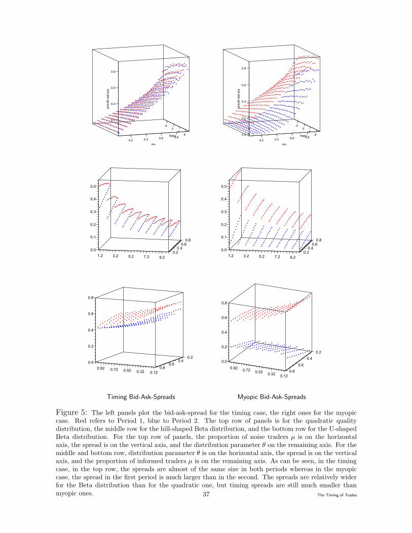
-40
theta4
80.80.6
mu
0.40.2
0.2
0.4
bid-ask-spread
0.6
0.8
-40
theta4
80.80.6
mu
0.40.2
0.0
0.2
0.4
bid-ask-spread
0.6
0.8
0.80.6
0.40.01.2
0.1
3.2
0.2
5.2
0.3
7.2
0.4
9.2
0.5
0.2
0.80.6
0.40.01.2
0.1
3.2
0.2
5.2
0.3
7.2
0.4
9.2
0.5
0.2
0.20.40.0
0.2
0.92
0.4
0.6
0.720.6
0.8
0.52 0.32 0.120.8
0.2
0.40.0
0.92
0.2
0.720.6
0.4
0.52
0.6
0.32
0.8
0.120.8
Timing Bid-Ask-Spreads Myopic Bid-Ask-Spreads
Figure 5: The left panels plot the bid-ask-spread for the timing case, the right ones for the myopiccase. Red refers to Period 1, blue to Period 2. The top row of panels is for the quadratic qualitydistribution, the middle row for the hill-shaped Beta distribution, and the bottom row for the U-shapedBeta distribution. For the top row of panels, the proportion of noise traders µ is on the horizontalaxis, the spread is on the vertical axis, and the distribution parameter θ on the remaining axis. For themiddle and bottom row, distribution parameter θ is on the horizontal axis, the spread is on the verticalaxis, and the proportion of informed traders µ is on the remaining axis. As can be seen, in the timingcase, in the top row, the spreads are almost of the same size in both periods whereas in the myopiccase, the spread in the first period is much larger than in the second. The spreads are relatively widerfor the Beta distribution than for the quadratic one, but timing spreads are still much smaller thanmyopic ones. 37 The Timing of Trades
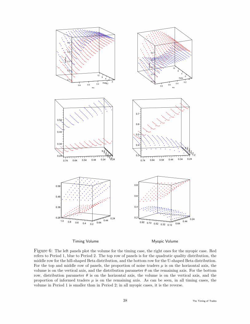
128
4
theta0
-40.20.4
mu
0.60.8
0.1
0.2
0.3
volume
0.4
0.5
128
4
theta0
-4
0.20.4
mu0.6
0.8
0.2
0.3
0.4volume
0.5
0.6
9.27.25.23.21.20.240.340.440.540.640.74
0.24
0.34
0.44
0.54
9.27.25.23.21.2
0.240.340.440.540.640.74
0.3
0.4
0.5
0.6
0.7
0.240.44
0.281.0
0.38
0.48
0.8
0.58
0.6 0.640.4 0.2
0.240.44
0.2
0.4
0.92
0.6
0.8
0.72 0.52 0.640.32 0.12
Timing Volume Myopic Volume
Figure 6: The left panels plot the volume for the timing case, the right ones for the myopic case. Redrefers to Period 1, blue to Period 2. The top row of panels is for the quadratic quality distribution, themiddle row for the hill-shaped Beta distribution, and the bottom row for the U-shaped Beta distribution.For the top and middle row of panels, the proportion of noise traders µ is on the horizontal axis, thevolume is on the vertical axis, and the distribution parameter θ on the remaining axis. For the bottomrow, distribution parameter θ is on the horizontal axis, the volume is on the vertical axis, and theproportion of informed traders µ is on the remaining axis. As can be seen, in all timing cases, thevolume in Period 1 is smaller than in Period 2; in all myopic cases, it is the reverse.
38 The Timing of Trades
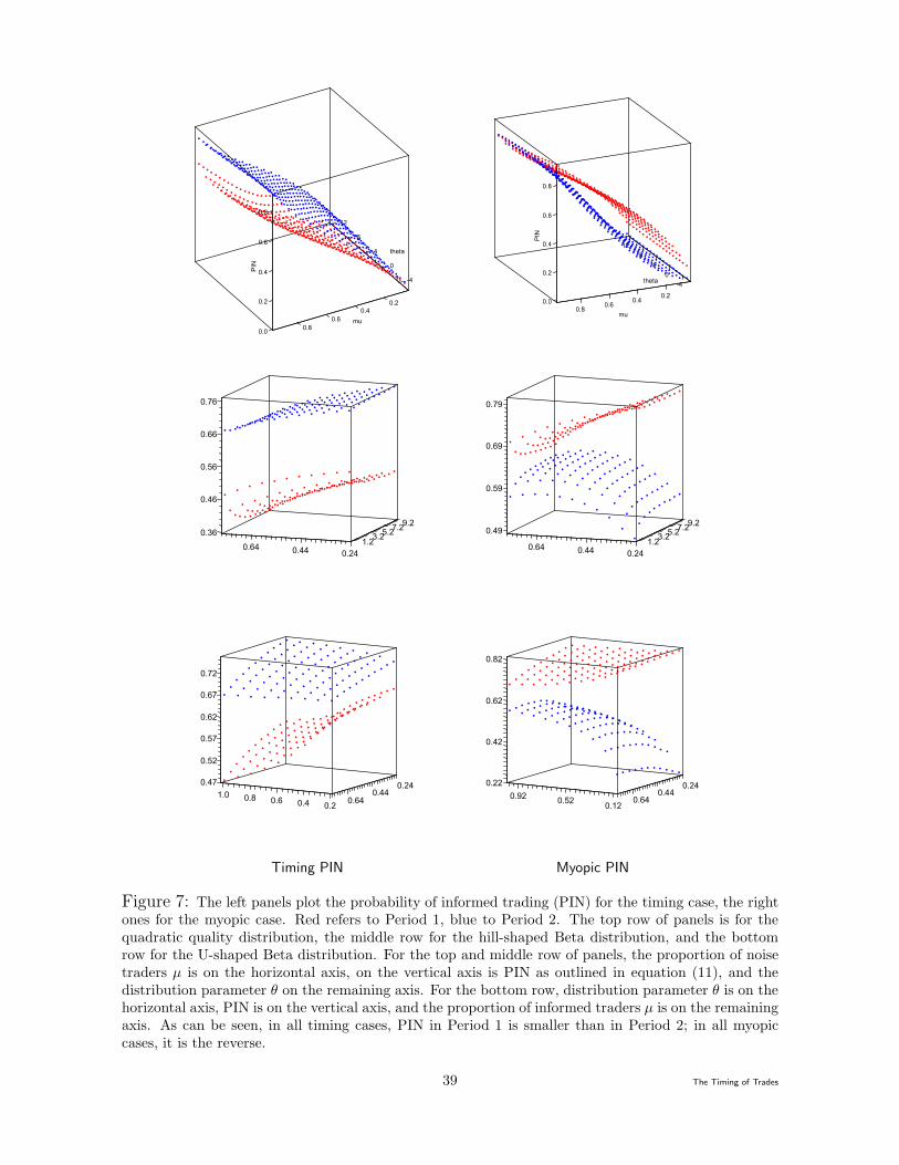
12
8
4 theta
0
-4
0.20.4
0.6 mu0.80.0
0.2
0.4PIN
0.6
0.8
128
4
theta0
-4
0.20.4
mu0.6
0.80.0
0.2
0.4
PIN
0.6
0.8
9.27.25.20.36
0.46
0.64
0.56
0.66
3.2
0.76
0.441.2
0.24
9.27.25.20.49
0.59
0.64
0.69
3.2
0.79
0.441.2
0.24
0.240.44
0.471.0
0.52
0.57
0.62
0.67
0.8
0.72
0.6 0.640.4 0.2
0.240.44
0.22
0.42
0.92
0.62
0.82
0.52 0.640.12
Timing PIN Myopic PIN
Figure 7: The left panels plot the probability of informed trading (PIN) for the timing case, the rightones for the myopic case. Red refers to Period 1, blue to Period 2. The top row of panels is for thequadratic quality distribution, the middle row for the hill-shaped Beta distribution, and the bottomrow for the U-shaped Beta distribution. For the top and middle row of panels, the proportion of noisetraders µ is on the horizontal axis, on the vertical axis is PIN as outlined in equation (11), and thedistribution parameter θ on the remaining axis. For the bottom row, distribution parameter θ is on thehorizontal axis, PIN is on the vertical axis, and the proportion of informed traders µ is on the remainingaxis. As can be seen, in all timing cases, PIN in Period 1 is smaller than in Period 2; in all myopiccases, it is the reverse.
39 The Timing of Trades
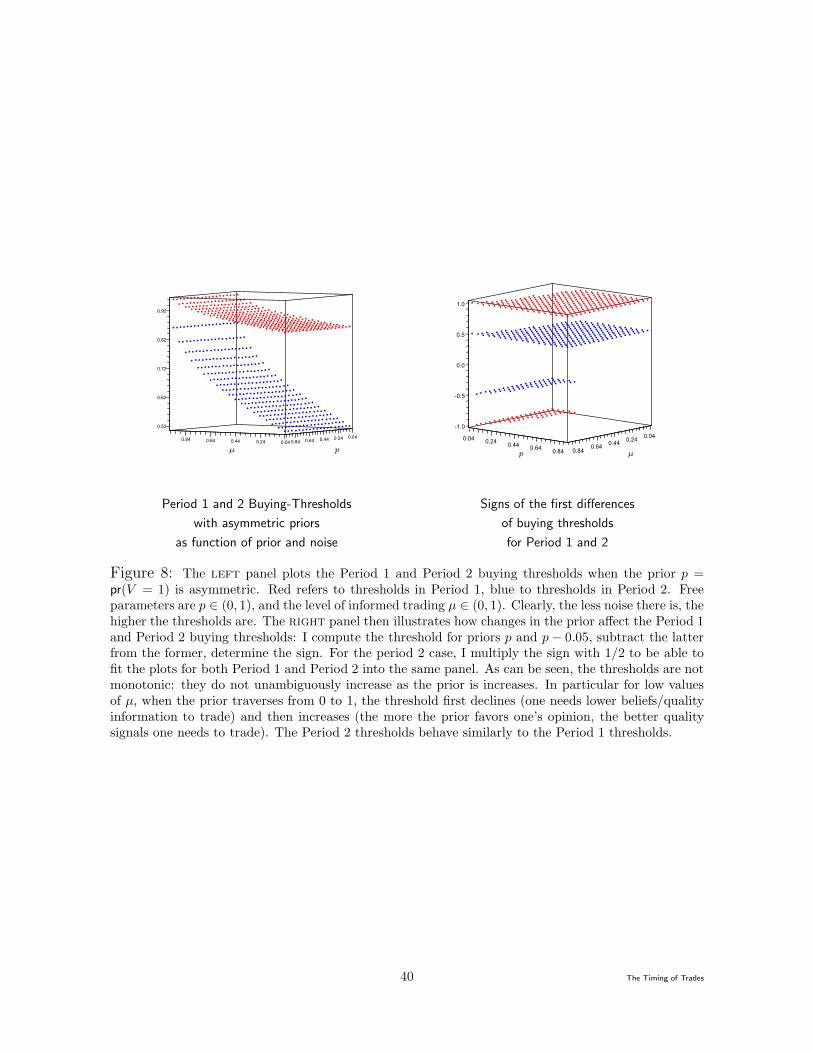
0.040.24
π
0.52
0.62
0.72
0.44
0.82
0.92
ρ
0.84 0.64 0.64
µ0.44 0.840.24 0.04
pµ
0.040.04
-1.0
0.24
-0.5
0.0
0.24
0.5
π
1.0
0.44
µ
0.44
ρ
0.640.64 0.840.84 µp
Period 1 and 2 Buying-Thresholds
with asymmetric priors
as function of prior and noise
Signs of the first differences
of buying thresholds
for Period 1 and 2
Figure 8: The left panel plots the Period 1 and Period 2 buying thresholds when the prior p =pr(V = 1) is asymmetric. Red refers to thresholds in Period 1, blue to thresholds in Period 2. Freeparameters are p ∈ (0, 1), and the level of informed trading µ ∈ (0, 1). Clearly, the less noise there is, thehigher the thresholds are. The right panel then illustrates how changes in the prior affect the Period 1and Period 2 buying thresholds: I compute the threshold for priors p and p − 0.05, subtract the latterfrom the former, determine the sign. For the period 2 case, I multiply the sign with 1/2 to be able tofit the plots for both Period 1 and Period 2 into the same panel. As can be seen, the thresholds are notmonotonic: they do not unambiguously increase as the prior is increases. In particular for low valuesof µ, when the prior traverses from 0 to 1, the threshold first declines (one needs lower beliefs/qualityinformation to trade) and then increases (the more the prior favors one’s opinion, the better qualitysignals one needs to trade). The Period 2 thresholds behave similarly to the Period 1 thresholds.
40 The Timing of Trades


