
f
Vitaly Golubev
Biofuel quality control by portable XRF-analyser
Bachelor’s Thesis Environmental Engineering
May 2015
DESCRIPTION
Date of the bachelor's thesis
May 11th, 2015
Author(s)
Vitaly Golubev (email: [email protected])
Degree programme and option
Environmental Engineering (B Eng)
Name of the bachelor's thesis
Biofuel quality control by portable XRF-analyser Abstract
The objective of this thesis project was to find out feasibility of using a handheld XRF-analyser in solid biofuel quality control, particularly for recovered wood. Global biomass supply is estimated to grow rapidly, creating demand for automatic quality control systems. X-ray fluorescent technology brings about quick, accurate and non-destructive elemental analysis. Recovered wood fuel is challenging for combustion due to high levels of contaminants. During this work a list of challenging chemical elements in recovered wood fuel was created after reviewing relevant EU standards. XRF technology has its limitations. Effects of limitations that are dependent on analysed samples were practically examined with an experimental XRF set-up built in a laboratory. As a result of the tests, it was found that increasing the XRF analysis time did not considerably improve the detected elemental concentrations. However an air gap between the analyser and a sample significantly decreased measured concentrations. Wood moisture also reduced detected concentrations although it could be possible to mathematically correct this effect if knowing the moisture content level. Another important finding was that analysing wooden matrix by hand with a handheld XRF-analyser posed health risks even if a backscatter shield was used, due to high dose rates of radiation scattered off the sample into surroundings. In the conclusion, a handheld XRF-analyser can be utilised in solid biofuel quality control. Its accuracy can be further increased by compensating negative effects of known limitations. Subject headings, (keywords)
XRF, analysis, biofuel, recovered wood, quality control, limitations, testing. Pages Language URN
51
English
Remarks, notes on appendices
Tutor
Aila Puttonen
Employer of the bachelor's thesis
Mika Muinonen
Inray Oy Ltd (www.inray.fi)
CONTENTS
LIST OF ABBREVIATIONS ..................................................................................................... 1
1 INTRODUCTION ............................................................................................................ 2
2 GLOBAL BIOFUEL PRODUCTION ............................................................................. 3
3 RECOVERED WOOD FUEL ......................................................................................... 4
3.1 Characteristics ......................................................................................................... 4
3.2 EN classification ..................................................................................................... 5
3.3 Challenging chemical elements ............................................................................ 10
4 XRF TECHNOLOGY .................................................................................................... 12
4.1 X-Ray Fluorescence principle ............................................................................... 12
4.2 Handheld XRF-analyser ........................................................................................ 13
4.3 Limitations of XRF analysis ................................................................................. 14
4.4 Online XRF applications in wood fuel processing ............................................... 18
5 METHODS USED IN THIS STUDY ............................................................................ 19
6 PRACTICAL TEST RESULTS ..................................................................................... 24
6.1 Particle size and chemical composition ................................................................ 24
6.2 Measurement time ................................................................................................ 26
6.3 Measurement distance........................................................................................... 28
6.4 Wood moisture...................................................................................................... 37
6.5 Radiation safety .................................................................................................... 44
7 CONCLUSIONS ............................................................................................................ 46
REFERENCES ......................................................................................................................... 48

1
LIST OF ABBREVIATIONS
CCA Chromated Copper Arsenate
DIY Do It Yourself
EDXRF Energy Dispersive X-Ray Fluorescence
GOLDD Geometrically Optimized Large Drift Detector
LOD Limits of Detection
MDF Medium Density Fibreboard
OSB Oriented Strand Board
PAS Publicly Available Specification
RWW Recovered Waste Wood
SDD Silicon Drift Detector
SRF Solid Recovered Fuel
WDXRF Wavelength Dispersive X-Ray Fluorescence
WRAP Waste and Resources Action Programme in United Kingdom
XRF X-Ray Fluorescence
2
1 INTRODUCTION
Biomass has long been used for global heating. Combustion of biomass produces fewer
emissions compared to fossil fuels, and it poses less ecological impacts. It can also be argued
that biomass can be seen as a renewable source of energy. Understandably, biomass is
increasingly becoming an important part of energy supply, especially for industrial uses.
In 2009, biomass shared 10,2 % of global energy supply, of which 13,5 % were used in
industrial production of heat and power (Vakkilainen et al. 2013). It is estimated that by 2030
the demand for biomass will double (International renewable energy agency 2014). Therefore,
more trade of biofuels will take place, and consequently, there will be a greater need for
technologies to assess biomass quality.
Suppliers of solid biofuel are bound to provide specifications of their product. However, often
fuel is sold for a higher price than its actual market value, for example, due to a greater
concentration of pollutants than provided in the specifications. Therefore, there is a great
interest and demand for equipment that could provide a fast and reliable fuel quality control.
An existing technology for solid fuel quality control is to send fuel samples to a laboratory for
analysis. It is time-consuming and may be expensive in a long term. The X-ray Fluorescence
(XRF) technology brings about high quality, fast and non-destructive measurements of fuel
samples on site.
This thesis project was a preliminary study on feasibility of using a handheld XRF-analyser
for solid biofuel quality control, particularly for recovered demolition wood. The thesis
consisted of theory and practical work. The theory covered an overview of global bioenergy
production, properties of recovered wood fuel and its classifications, description of the XRF
technology, its limitations and current applications in solid biofuel quality control. The theory
was obtained from previous publications and research as well as from different public web-
resources of XRF-equipment manufacturers. The practical work was done with a handheld
XRF-analyser in a laboratory at Mikkeli University of Applied Sciences, Finland. The aim
was to test how measurement time, distance to a sample, and wood moisture affected the
results of XRF analysis. The radiation rate doses during the testing were checked, and
radiation safety was ensured. The thesis was commissioned by Inray Oy Ltd company.
3
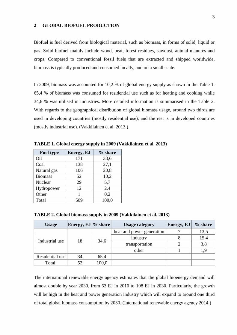
2 GLOBAL BIOFUEL PRODUCTION
Biofuel is fuel derived from biological material, such as biomass, in forms of solid, liquid or
gas. Solid biofuel mainly include wood, peat, forest residues, sawdust, animal manures and
crops. Compared to conventional fossil fuels that are extracted and shipped worldwide,
biomass is typically produced and consumed locally, and on a small scale.
In 2009, biomass was accounted for 10,2 % of global energy supply as shown in the Table 1.
65,4 % of biomass was consumed for residential use such as for heating and cooking while
34,6 % was utilised in industries. More detailed information is summarised in the Table 2.
With regards to the geographical distribution of global biomass usage, around two thirds are
used in developing countries (mostly residential use), and the rest is in developed countries
(mostly industrial use). (Vakkilainen et al. 2013.)
TABLE 1. Global energy supply in 2009 (Vakkilainen et al. 2013)
Fuel type Energy, EJ % share
Oil 171 33,6
Coal 138 27,1
Natural gas 106 20,8
Biomass 52 10,2
Nuclear 29 5,7
Hydropower 12 2,4
Other 1 0,2
Total 509 100,0
TABLE 2. Global biomass supply in 2009 (Vakkilainen et al. 2013)
Usage Energy, EJ % share Usage category Energy, EJ % share
Industrial use 18 34,6
heat and power generation 7 13,5
industry 8 15,4
transportation 2 3,8
other 1 1,9
Residential use 34 65,4
Total: 52 100,0
The international renewable energy agency estimates that the global bioenergy demand will
almost double by year 2030, from 53 EJ in 2010 to 108 EJ in 2030. Particularly, the growth
will be high in the heat and power generation industry which will expand to around one third
of total global biomass consumption by 2030. (International renewable energy agency 2014.)
4
3 RECOVERED WOOD FUEL
Recovered wood fuel is defined as wood material received from different categories of waste
as fuel for heat or electricity generation. Wood waste sources may be grouped into 3 sectors:
domestic sector, construction and demolition sector, and commercial and industrial sector
(wooden packaging, wood products manufacture, treated timber products). (PAS 111:2012.)
3.1 Characteristics
Solid recovered fuel (SRF) includes all material mixes that can be incinerated and are certified
according to the EN 15359 standard “Solid recovered fuels – specifications and classes”. The
source of SRF is mainly municipal solid waste, commercial and industrial wastes. Typical
composition of SRF is as follows (in wet weight %): paper: 40-50 %, plastics: 25-35 %, and
textiles: 10-14 %. In literature, solid recovered fuel category often includes recovered wood
fuels. (Bankiewicz 2012; Jones 2013.)
Recovered waste wood (RWW) is all wood-based material which originates from waste and is
intended to be processed for further use. It mainly comes from construction and demolition
processes. In addition to wood material, RWW typically contains metal parts (nails, wires),
plastics (flooring, electrical wires), paints and wood preservation treatments (CCA, creosote).
The Table 3 below summaries different contaminants found in recovered waste wood.
(Bankiewicz 2012; Jones 2013.)
TABLE 3. Recovered waste wood contaminants (Bankiewicz 2012)
Contaminant Share, wet weight %
Surface treated wood 15
Preservative treated wood 3,5
Soil 0,6
Plastics 0,1
Iron, steel 0,5
Concrete 0,05
With regards to the chemical composition, RWW is problematic due to the high concentration
of heavy metals, particularly Cr, Cu, Zn, Cd, Hg, Pb. Paints, lacquers, binders and
preservatives contribute to the problem of heavy metals the most. SRF is reported to be high
in chlorine and bromine because of plastics present in the fuel made from municipal waste.
(Bankiewicz 2012, Vainikka 2011; Jones 2013.)
5
3.2 EN classification
This chapter is divided into 3 parts where each part is a review of a standard for solid biofuel
classification. Firstly, EN ISO 17225-1:2014 focuses on classification and specification of
biofuel with amount of halogenated organic compounds and heavy metals not exceeding the
values of virgin wood. Secondly, EN 15359 gives classification for solid recovered fuel.
Lastly, a specification PAS 111:2012 (UK) is also described.
EN ISO 17225-1:2014
The recent standard EN ISO 17225-1:2014 on specifications and classes of solid biofuels is
binding for the European Committee for Standardization (CEN) members to adopt it to their
national legislation. The standard is only intended for solid biofuels, including chemically
treated wood, that do not contain halogenated organic compounds or heavy metals in amounts
greater than those of typical virgin wooden material or virgin wooden material of a place of
wood origin. If these elements exceed the norm, then the standard EN 15359 should be used
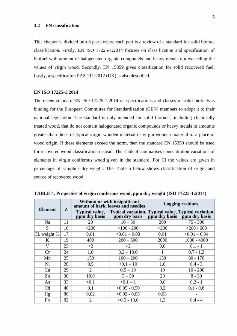
for recovered wood classification instead. The Table 4 summarises concentration variations of
elements in virgin coniferous wood given in the standard. For Cl the values are given in
percentage of sample’s dry weight. The Table 5 below shows classification of origin and
source of recovered wood.
TABLE 4. Properties of virgin coniferous wood, ppm dry weight (ISO 17225-1:2014)
Element Z
Without or with insignificant amount of bark, leaves and needles
Logging residues
Typical value, ppm dry basis
Typical variation, ppm dry basis
Typical value, ppm dry basis
Typical variation, ppm dry basis
Na 11 20 10 – 50 200 75 - 300
S 16 <200 <100 - 200 <200 <200 - 600
Cl, weight % 17 0,01 <0,01 – 0,03 0,01 <0,01 – 0,04
K 19 400 200 – 500 2000 1000 - 4000
V 23 <2 <2 0,6 0,1 - 1
Cr 24 1,0 0,2 – 10,0 1 0,7 - 1,2
Mn 25 150 100 – 200 130 80 - 170
Ni 28 0,5 <0,1 – 10 1,6 0,4 - 3
Cu 29 2 0,5 – 10 10 10 - 200
Zn 30 10,0 5 – 50 20 8 - 30
As 33 <0,1 <0,1 – 1 0,6 0,2 - 1
Cd 48 0,1 <0,05 - 0,50 0,2 0,1 - 0,8
Hg 80 0,02 <0,02 - 0,05 0,03 -
Pb 82 2 <0,5 - 10,0 1,3 0,4 - 4

6
According to the EN ISO 17225-1:2014, specification of solid biofuels includes normative
(compulsory) and informative (voluntary) properties. There are several criteria to specify solid
biofuels:
1. origin;
2. traded form;
3. properties such as dimensions, moisture and ash contents.
Normative properties to be stated depend on the origin and traded form.
TABLE 5. Classification of origin and sources of recovered wood (ISO 17225-1:2014)
Origin Source Sub-source
1.2. By-products
and residues
from wood
processing
industry
1.2.1. Chemically untreated
wood by-products and
residues
1.2.1.1 Broad-leaf with bark
1.2.1.2 Coniferous with bark
1.2.1.3 Broad-leaf with bark
1.2.1.4 Coniferous with bark
1.2.1.5. Bark (from industry operation)
1.2.2. Chemically treated
wood by-products, residues,
fibres and wood constitutes
1.2.2.1. Without bark
1.2.2.2. With bark
1.2.2.3. Bark (from industry operation)
1.2.2.4. Fibres and wood constituents
1.2.3. Blends and mixtures
1.3. Used wood
1.3.1 Chemically untreated
used wood
1.3.1.1 Without bark
1.3.1.2. With bark
1.3.1.3. Bark
1.3.2. Chemically treated
used wood
1.3.2.1. Without bark
1.3.2.2. With bark
1.3.2.3. Bark
1.3.3. Blends and mixtures
The EN ISO 17225-1:2014 gives 21 major traded forms of solid biofuels and their typical
particle sizes. Among them are wood chips (5 mm – 100 mm), hog fuel (varying size),
logwood (50 cm – 100 cm), firewood (5 cm – 100 cm) and sawdust (1 mm – 5 mm).
However, other forms which are not included in the standard are also possible to be used.
Specification of fuel properties is dependent on fuel’s origin and traded form. For example,
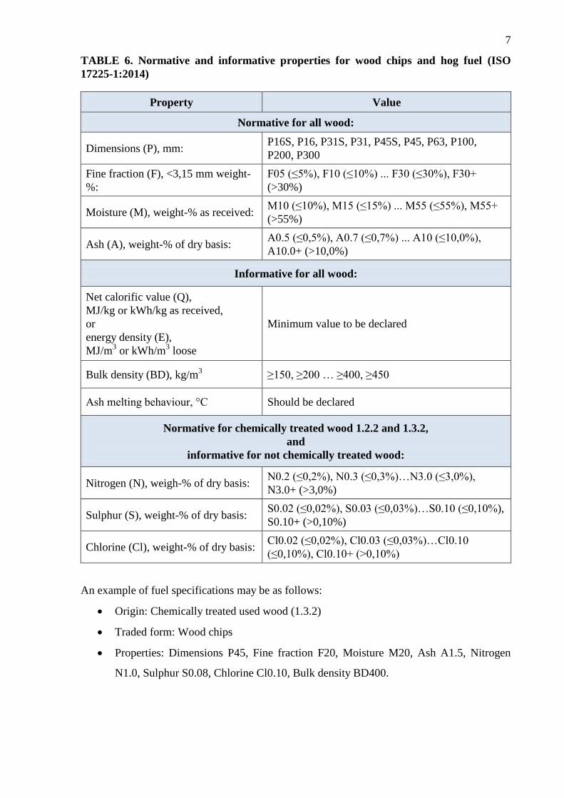
properties for wood chips and hog fuel are listed in the Table 6 below.
7
TABLE 6. Normative and informative properties for wood chips and hog fuel (ISO
17225-1:2014)
Property Value
Normative for all wood:
Dimensions (P), mm: P16S, P16, P31S, P31, P45S, P45, P63, P100,
P200, P300
Fine fraction (F), <3,15 mm weight-
%:
F05 (≤5%), F10 (≤10%) ... F30 (≤30%), F30+
(>30%)
Moisture (M), weight-% as received: M10 (≤10%), M15 (≤15%) ... M55 (≤55%), M55+
(>55%)
Ash (A), weight-% of dry basis: A0.5 (≤0,5%), A0.7 (≤0,7%) ... A10 (≤10,0%),
A10.0+ (>10,0%)
Informative for all wood:
Net calorific value (Q),
MJ/kg or kWh/kg as received,
or
energy density (E),
MJ/m3 or kWh/m
3 loose
Minimum value to be declared
Bulk density (BD), kg/m3 ≥150, ≥200 … ≥400, ≥450
Ash melting behaviour, °C Should be declared
Normative for chemically treated wood 1.2.2 and 1.3.2,
and
informative for not chemically treated wood:
Nitrogen (N), weigh-% of dry basis: N0.2 (≤0,2%), N0.3 (≤0,3%)…N3.0 (≤3,0%),
N3.0+ (>3,0%)
Sulphur (S), weight-% of dry basis: S0.02 (≤0,02%), S0.03 (≤0,03%)…S0.10 (≤0,10%),
S0.10+ (>0,10%)
Chlorine (Cl), weight-% of dry basis: Cl0.02 (≤0,02%), Cl0.03 (≤0,03%)…Cl0.10
(≤0,10%), Cl0.10+ (>0,10%)
An example of fuel specifications may be as follows:
Origin: Chemically treated used wood (1.3.2)
Traded form: Wood chips
Properties: Dimensions P45, Fine fraction F20, Moisture M20, Ash A1.5, Nitrogen
N1.0, Sulphur S0.08, Chlorine Cl0.10, Bulk density BD400.
8
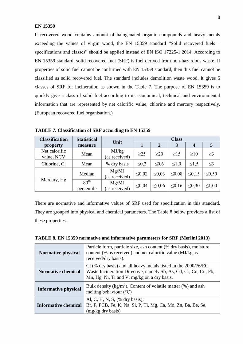
EN 15359
If recovered wood contains amount of halogenated organic compounds and heavy metals
exceeding the values of virgin wood, the EN 15359 standard “Solid recovered fuels –
specifications and classes” should be applied instead of EN ISO 17225-1:2014. According to
EN 15359 standard, solid recovered fuel (SRF) is fuel derived from non-hazardous waste. If
properties of solid fuel cannot be confirmed with EN 15359 standard, then this fuel cannot be
classified as solid recovered fuel. The standard includes demolition waste wood. It gives 5
classes of SRF for incineration as shown in the Table 7. The purpose of EN 15359 is to
quickly give a class of solid fuel according to its economical, technical and environmental
information that are represented by net calorific value, chlorine and mercury respectively.
(European recovered fuel organisation.)
TABLE 7. Classification of SRF according to EN 15359
Classification
property
Statistical
measure Unit
Class
1 2 3 4 5
Net calorific
value, NCV Mean
MJ/kg
(as received) ≥25 ≥20 ≥15 ≥10 ≥3
Chlorine, Cl Mean % dry basis ≤0,2 ≤0,6 ≤1,0 ≤1,5 ≤3
Mercury, Hg
Median Mg/MJ
(as received) ≤0,02 ≤0,03 ≤0,08 ≤0,15 ≤0,50
80th
percentile
Mg/MJ
(as received) ≤0,04 ≤0,06 ≤0,16 ≤0,30 ≤1,00
There are normative and informative values of SRF used for specification in this standard.
They are grouped into physical and chemical parameters. The Table 8 below provides a list of
these properties.
TABLE 8. EN 15359 normative and informative parameters for SRF (Merlini 2013)
Normative physical
Particle form, particle size, ash content (% dry basis), moisture
content (% as received) and net calorific value (MJ/kg as
received/dry basis).
Normative chemical
Cl (% dry basis) and all heavy metals listed in the 2000/76/EC
Waste Incineration Directive, namely Sb, As, Cd, Cr, Co, Cu, Pb,
Mn, Hg, Ni, Ti and V, mg/kg on a dry basis.
Informative physical Bulk density (kg/m
3), Content of volatile matter (%) and ash
melting behaviour (°C)
Informative chemical
Al, C, H, N, S, (% dry basis);
Br, F, PCB, Fe, K, Na, Si, P, Ti, Mg, Ca, Mo, Zn, Ba, Be, Se,
(mg/kg dry basis)

9
PAS 111:2012
PAS 111:2012 is a Publicly Available Specification (PAS) designed to provide producers and
end-users of waste wood in the United Kingdom with a tool to classify wood into several
categories based on its quality. Waste wood is defined as any type of wood that has been
discarded or is intended to be discarded. It should be noted that the PAS 111 is not a British
standard, and other restrictions may apply such as from the 2000/76/EC Waste Incineration
Directive. The Table 9 below summarises information on how to give a grade to waste wood.
According to PAS 111:2012, there are 4 classification grades of waste wood:
“grade A” Clean recycled wood,
“grade B” Industrial feedstock,
“grade C” Fuel,
“grade D” Hazardous waste.
TABLE 9. Grades of waste wood (PAS 111:2012)
Grade Description
A
Solid softwood and hardwood. Packaging waste, scrap pallets, packing cases and
cable drums. Residues from the production of untreated product.
May contain nails and metal fixings. Minor amounts of paint, and surface coatings.
B
May have 60 % of grade “A” material, plus building and demolition material and
domestic furniture made from solid wood.
May contain nails and metal fixings. Some paints, plastics, glass, grit, coatings,
binders and glues. Limits on treated or coated materials as defined by the Waste
Incineration Directive.
C
All materials given in “A” and “B” grades, plus fencing products, flat pack
furniture made from board products and DIY materials. High content of panel
products such as chipboard, MDF, plywood, OSB and fibreboard.
May contain nails and metal fixings. Paints coatings and glues, paper, plastics and
rubber, glass, grit as well as coated and treated timber (but non CCA or creosote)
D
Fencing, transmission poles, railway sleepers, cooling towers.
Contains material with CCA treatment and creosote.
The following abbreviations are used the Table 9:
DIY – Do It Yourself
MDF - Medium Density Fibreboard
OSB - Oriented Strand Board
CCA - Chromated Copper Arsenate

10
3.3 Challenging chemical elements
Totally 19 elements of interest have been identified. Of those, 4 elements (Na, K, Br and Zn)
are included due to their corrosive effect during combustion as found on literature reviews,
and the other 15 elements are mandatory for solid biofuel quality assessment based on
recovered wood classifications from the previous chapter. The Table 10 lists the identified
elements and their source of information. Negative effects of several elements on combustion
reactors are also discussed below.
TABLE 10. Elements of interest for recovered wood fuel quality control
# Symbol Element name Atomic
number, Z Source of information
1 N Nitrogen 7 EN ISO 17225-1
2 Na Sodium 11 Bankiewicz 2012; Sandberg 2011
3 S Sulphur 16 EN ISO 17225-1
4 Cl Chlorine 17 EN 15359, EN ISO 17225-1
5 K Potassium 19 Bankiewicz 2012; Sandberg 2011
6 V Vanadium 23 EN 15359
7 Cr Chromium 24 EN 15359, PAS 111:2012
8 Mn Manganese 25 EN 15359
9 Co Cobalt 27 EN 15359
10 Ni Nickel 28 EN 15359
11 Cu Copper 29 EN 15359, PAS 111:2012
12 Zn Zinc 30 Bankiewicz 2012; Sandberg 2011
13 As Arsenic 33 EN 15359, PAS 111:2012
14 Br Bromine 35 Bankiewicz 2012; Vainikka 2011
15 Cd Cadmium 48 EN 15359
16 Sb Antimony 51 EN 15359
17 Hg Mercury 80 EN 15359
18 Tl Thallium 81 EN 15359
19 Pb Lead 82 EN 15359
Chlorine
Chlorine is considered to be the most dangerous element for combustion reactors. Chlorine is
common in biomass and present in relatively high concentration. At the superheated
temperature zone (600 – 700 °C) chlorine forms gaseous compounds such as HCl and Cl2
which react with iron and chromium in the reactor’s steel causing it to corrode. (Viklund
2013; Valmari 2000.)
11
Potassium and sodium
Potassium, being an important plant nutrient, is a dominant alkali metal in biomass followed
by sodium. In combustion reactor, they can react with chlorine to form very low melting
temperature compounds thus creating favourable conditions for ash and soot formation at
lower superheated temperatures. Ash causes fouling and corrosion of reactor’s surface.
(Bankiewicz 2012; Sandberg 2011.)
Bromine
Deposits of bromine compounds (KBr and NaBr) develop corrosion of boiler steel. Bromides
may cause high temperature corrosion of furnace’s steel as well corrosion of boiler surface at
low temperatures more extensively than caused by chlorides. (Bankiewicz 2012; Vainikka
2011.)
Lead and zinc
Lead and zinc are both heavy metals, and they can react with chlorine and sulphur in a
combustion reactor forming salt mixtures that have a low melting temperature. Due to the low
melting temperature, they deposit on the boiler’s heat exchanging surfaces inducing fouling
and slagging as well as corrosive effects already at 300 – 400 °C. (Bankiewicz 2012;
Sandberg 2011.)
12
4 XRF TECHNOLOGY
X-ray Fluorescence (XRF) is widely used for a non-destructive elemental analysis. Compared
to other analytical techniques, XRF is fast and reliable, and it does not require sample
preparation. Samples do not need to be dissolved or destroyed in other ways. There are Energy
Dispersive and Wavelength Dispersive XRF-analysers, and they differ considerably in their
properties. However, the XRF technology has its limitations, and thus it is essential to know
when and how an XRF analysis may give incorrect measurement results.
4.1 X-Ray Fluorescence principle
X-ray fluorescence is a phenomenon observed when an X-ray shines on material and generates
a secondary X-ray, called fluorescent. The Figure 1 below schematically illustrates the XRF
principle. A primary X-ray originated from an X-ray source is beamed at the material sample
and accidentally hits an electron in an atom, e.g. on the K-shell. This electron is ejected from
its electron shell creating a vacant place which is immediately occupied by an electron from a
higher energy shell, e.g. L-shell or M-shell. When the electron makes the transition between
the shells, a photon is emitted forming electromagnetic radiation, namely fluorescent X-
radiation. The fluorescent X-ray carries energy unique to each chemical element, therefore by
examining the energy level it is possible to understand the elemental composition of the
sample. The XRF technology utilises such principle to analyse materials. (Amptek Inc.)
FIGURE 1. X-ray fluorescence principle
Na
K L M
X-ray source
Primary X-ray
Fluorescent X-ray
Ejected electron
13
Additional letters alpha (α), beta (β) and gamma (γ) are used to classify the originating
electron shell of fluorescent X-rays. An X-ray Kα is formed during the electron transition
from the L-shell to the K-shell. An X-ray Kβ is created during the electron transition from the
M-shell to the K-shell. Similarly, an X-ray Lα is emitted during transition from the M-shell to
the L-shell. Moreover, there are several sub-levels in each electron shell, and every sub-level
is distinguished by numbering. Therefore, X-rays are given labels such as Kα1 and Lβ2 for
more detailed information on their origin. (Amptek Inc.)
4.2 Handheld XRF-analyser
The Niton XL3t 980 GOLDD+ is a handheld Energy Dispersive XRF-analyser (EDXRF)
manufactured by Thermo Fisher Scientific Inc. It features an X-ray tube of 50 kV and 200 μA
as an X-ray source as well as a large area Silicon Drift Detector (SDD) with resolution of less
than 185 eV at 60 000 counts per second (Thermo Fisher Scientific Inc). Its analytical range of
elements is from Mg to U. This portable XRF-analyser can be controlled either directly with a
touch screen or remotely with computer software. The Figure 2 below illustrates the location
of the X-ray tube and detector inside the analyser. Its software allows several analytical modes
by default, of which TestAll Geo was used in this study.
FIGURE 2. Handheld XRF detection principle (left), and Niton XL3t 980 (right)
CPU
X-ray source
Detector
Sample
14
Analyser’s radiation safety
In Finland, according to the guide on the “use of control and analytical X-ray apparatus”
available from the Finnish radiation and nuclear safety authority, the effective annual radiation
dose should not exceed 0,3 mSv. A human presence in the area with the dose rate over 1,5
μSv/h must be limited to one hour per day. Additionally, if the work is done in the area with
the dose rate over 5 μSv/h, special safety procedure should be made to restrict the annual
radiation dose to 0,3 mSv. (Finnish radiation and nuclear safety authority 2008.)
According to X-ray tube radiation survey certificate which is shipped along with the analyser,
maximum radiation dose rates measured for a steel sample are as follows: at 5 cm distance it
is 1,23 μSv/h while at 10 cm it is 0,36 μSv/h (Thermo Fisher Scientific Inc 2014).
4.3 Limitations of XRF analysis
Technologically, the XRF analysis gives different measurement results due to its limitations.
There are several aspects that should be taken into consideration when measuring a
concentration of particular elements.
Resolution of XRF equipment
The resolution of an XRF detector is a numerical value, measured in eV, which represents a
difference between the nearest spectra peaks (K or L shells) of elements that the detector can
recognise in a sample. For example, sodium has Kα = 1,040 keV and magnesium has Kα =
1,254 keV energies (Bruker). Their spectra peak difference is (1,254 - 1,040) keV = 0,214
keV, or 214 eV. If XRF equipment has a detector with a resolution greater than 214 eV, it will
be problematic to distinguish between these two elements. (US Environmental Protection
Agency 2004.)
There are 2 main types of XRF equipment architecture: Energy Dispersive XRF (EDXRF) and
Wavelength Dispersive XRF (WDXRF). Their difference lies in the structure, accuracy and
measurement time. The EDXRF is able to analyse the whole spectrum which is fast while the
WDXRF focuses only on one element at a time which is very time consuming. After
reviewing multiple XRF-analyser specifications from different manufacturers, it can be
summarised that regarding the resolution, EDXRF ranges from 150 eV to 300 eV and above,
while WDXRF has a resolution as low as 5 eV to 20 eV.

15
Elemental range
There is a range of elements that can be traced using the XRF technology. A typical EDXRF-
analyser can identify elements from sodium to uranium (Bruker 2012). In comparison, a
WDXRF-analyser is capable of distinguishing very light elements, from boron to uranium
(Bruker 2012). Using the EDXRF technology, elements lighter than sodium are not detectable
(Fellin et al. 2014), and elements lighter than argon are very difficult to detect because the
energy levels of their fluorescent X-rays are low and fluorescent photons are weakened by the
air gap between the sample and detector (Thermo Fisher Scientific Inc 2013). Because of
these low energies, the fluorescent photons can be ejected from the sample only if the targeted
atoms are close to the surface (Bruker 2008). Moreover, detectability of elements depends on
other factors such as matrix composition, sample moisture and duration of measurements.
Measurement time
The measurement time is a crucial limit of the XRF technology. The longer the analysis time
is, the more accurate the results are, because it produces more counts per second.
Mathematically, if the measurement time is n-times longer, then the limit of detection (LOD)
is improved SQRT(n)-times (Thermo Fisher Scientific Inc 2010). If a sample is analysed 4
times longer, the LOD will increase 2 times. Such dependence is also seen in the research
made by Fellin at el. (2014) on wooden matrix using an Oxford Instruments X-MET 5100
EDXRF-analyser with an X-ray source of 45 kV 40 μA. The Table 11 below shows minimum
detection limits of relevant to this study elements acquired from their work.
TABLE 11. Minimum detection limits (ppm) of elements in wood (Fellin et al. 2014)
Element Atomic
number, Z
Time, second
5 10 15 20 30 60 120 180 600
Cl 17 23000 16000 13000 11000 9000 7000 5000 4000 2000
K 19 20000 14000 12000 10000 8000 6000 4000 3000 2000
V 23 30 19 15 13 11 8 5 4 2
Cr 24 20 16 13 11 9 6 5 4 2
Mn 25 19 13 11 9 8 5 4 3 2
Co 27 15 11 9 8 6 4 3 3 1
Ni 28 15 10 8 7 6 4 3 2 1
Cu 29 23 16 13 11 9 7 5 4 2
Zn 30 20 14 12 10 8 6 4 3 2
As 33 12 9 7 6 5 4 3 2 1
Cd 48 29 21 17 15 12 8 6 5 3
Sb 51 59 42 34 29 24 17 12 10 5
Hg 80 3 2 2 1 1 0,8 0,6 0,5 0,3
Pb 82 2 2 1 1 1 0,7 0,5 0,4 0,2

16
Depth of analysis
There are 3 main variables that affect how deep X-rays penetrate a sample: energy of X-rays,
density of the sample material, and energy level of analysed element. Firstly, the greater the
energy of an X-ray photon from analyser is, the greater the measurement depth is.
Secondly, low density material matrix such as wood and plastic allow for a deeper X-ray
screening, compared to denser material. Low-energy X-rays are not able to enter a high-
density matrix and excite elements, while high-energy X-rays penetrate a low-density sample
much deeper (Wobrauschek et al. 2010; Anzelmo et al. 2014). For example, in the mining
industry, depending on a sample density, a typical range for XRF analysis is from several
microns to 9,5 mm (Thermo Fisher Scientific Inc 2009).
Thirdly, the analysis depth is different for each element due to the elemental excitation energy.
The higher the atomic energy of an element, the deeper it can be traced within a sample
(Guthrie 2012; Anzelmo et al. 2014). With regards to the thickness of wood analysis, Fellin et
al (2014) reported a maximum detection depth of copper (Cu) from 15 mm to 24 mm
depending on wooden matrix.
Distance to sample
The distance between an XRF-analyser and sample attenuates the number of fluorescent X-ray
photons (Wobrauschek et al. 2010). For the best performances it is suggested to have a direct
contact with tested material (US Environmental Protection Agency 2004; Thermo Fisher
Scientific Inc 2010). Naturally, having such a distance is crucial for online sorting systems
where wood comes in different shapes and sizes. Therefore there must be a gap between the
XRF-analyser and conveyer. In research on XRF analysis of CCA-treated wood conducted by
Solo-Gabriele et al (2003) it was recommended mounting the analyser at a most practical
distance of 19 mm above the belt, with the maximum distance for XRF being 30 mm.
Moisture
If the moisture of a sample is greater than 20 %, then it can negatively affect XRF-analysis
results. The reason is water contained in the sample, or on its surface, which serves as an
extra-barrier for X-rays. It is possible to calibrate an XRF analyser for more accurate analysis
after correction factors are determined with help of a dried sample in a laboratory. (US
Environmental Protection Agency 2004; Glanzman & Closs 2007.)
17
On the other hand, for CCA-treated wood, Solo-Gabriele et al. (2003) suggest that there was
no significant difference in detecting arsenic in a wet sample after 30 minutes of soaking it in
water compared to a dry sample (during 3 second test with a 19 mm air gap).
Particle size
Firstly, in natural matrix elements are not distributed equally, therefore large particles do not
represent the whole sample. Secondly, heterogeneous matrix scatters fluorescent X-rays away
from the XRF-detector which lowers the quantitative results of analysis. Graining to fine
particles and making a homogeneous sample is highly recommended in order to acquire more
accurate results. In case of fine homogeneous matrix, the X-rays could reach particles that are
hidden behind the top particles’ layer therefore making a more representative analysis.
(Thermo Fisher Scientific Inc 2013; Anzelmo et al. 2014; Glanzman & Closs 2007.)
Spectral matrix effect
In addition to the above described limitations, there are 3 more that can cause false XRF-
analyser’s readings. Namely, those effects are overlapping, enhancement and absorption.
Overlapping of spectral lines occurs when analysed elements emit fluorescent photons of
similar wavelength. For example, lead L-peak overlaps with arsenic K-peak. Moreover, if a
proportion of lead to arsenic is at least 10:1, then concentration of arsenic cannot be measured
adequately due to a complete overlap. (US Environmental Protection Agency 2004.)
During the enhancement, an XRF-analyser can show a higher concentration of several
elements because their binding elemental energies are less than those of fluorescent X-rays of
other elements present in a sample. In addition to the analyser’s X-ray source, these
fluorescent X-rays become a secondary source of X-rays for the elements with lower
elemental energies. An example of this can be chromium enhanced by iron. (Thermo Fisher
Scientific Inc 2013; US Environmental Protection Agency 2004.)
Lastly, there are several elements that absorb or scatter fluorescent X-rays of other elements,
as it is in the case of iron absorbing copper fluorescent X-rays. The absorption causes an XRF-
analyser to show lower concentration values of elements than there really are in the sample.
Computer software of the analyser is designed to effectively correct these limitations.
(Thermo Fisher Scientific Inc 2013; US Environmental Protection Agency 2004.)
18
4.4 Online XRF applications in wood fuel processing
Online XRF-systems are widely used in mining industry for quality assessment of extracted
ores (Nakhaei et al. 2012). However, full-scale working implementations of online XRF-
systems in wood fuel processing have not been found. There is a limited number of studies on
online wood fuel XRF-analysis. Notably, a pilot project carried out by Solo-Gabriele et al
(2001) for the Sarasota county, USA, looked at XRF-analysis for sorting of CCA-treated
wood. It was found that XRF technology can be effectively used to detect CCA-treated wood
from other types of wood pieces on a moving conveyer. One limitation of online measurement
is that an XRF-analyser should be mounted above the belt at a distance thus reducing the
quality of results. Moreover, a slow speed of XRF-analysis is also a limit because it slows
down the conveyer and minimises the amount of analysed wood per given time. As a result,
the optimal height above a belt was 19 mm, and the minimum sufficient time was 3 seconds.
The measurement time can be dramatically reduced to milliseconds if the XRF-analyser is
built specifically for online measurement and its shatter is constantly open. In addition,
although paints, coating and stains on wood pieces were found to reduce number of As
fluorescent X-ray counts, CCA-treated wood was still detectable. (Solo-Gabriele et al. 2001.)
Another field trial research on online sorting of treated wood was done in cooperation of
Pöyry Forest Industry Consulting Ltd and Waste and Resources Action Programme in the UK,
2009. In online analysis, XRF technology was capable of identifying Cu in Tanalith treated
wood with concentration above 40 mg/kg at 2,7 seconds on average. For CCA-treated wood,
it was found that As and Cr will be easily traced with XRF while Cu analysis gave too high
uncertainties for conclusive results at 6,2 second measurement time. Detection of clean wood
takes long time duration (up to 30 seconds). As the concentration of elements increases, the
analysis time decreases. In the end, as the report suggests, it is questionable if XRF technology
can be effectively applied to an online recovered wood sorting of recovered wood due to the
distance between an XRF-analyser and wood on a conveyer, different shapes of wood pieces
and a long analysis time required. (Waste and Resources Action Programme 2009.)
19
5 METHODS USED IN THIS STUDY
The practical tests formed a preliminary study on XRF-analysis of recovered wood with
emphasis on simulating conditions for an on-line XRF system. The limitations of the XRF
technology were tested and observed, particularly, how length of analysis, measurement
distance to a sample, and wood moisture affect results of the XRF-analyses.
The Niton XL3t 980 GOLDD+ analyser was fixed on a laboratory stand which allowed
moving the device vertically with a 2 mm step. A backscatter shield was attached to the
analyser. The analyser was remotely controlled with software on a laptop. In the beginning of
the practical work radiation levels near the XRF-analyser were measured with a radiation
detection meter because, being low-density material, wood did not absorb X-rays very well,
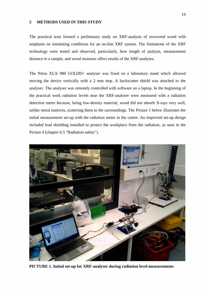
unlike metal matrices, scattering them to the surroundings. The Picture 1 below illustrates the
initial measurement set-up with the radiation meter in the centre. An improved set-up design
included lead shielding installed to protect the workplace from the radiation, as seen in the
Picture 4 (chapter 6.5 “Radiation safety”).
PICTURE 1. Initial set-up for XRF-analyser during radiation level measurements
20
For the radiation measurement, oven-dried wood chips in a plastic bag were chosen as a
sample. The plastic bag was used because it was noticed that most of XRF analyses in the
laboratory were done with plastic bags. The radiation check points were at 1 cm, 40 cm, 80
cm, and 120 cm distance to the analyser. The radiation detection meter was placed on a
laboratory jack stand at the same height as the analysed sample, as seen in the Picture 1 above.
Two sets of measurement were performed: when the analyser contacted the sample and when
it was 2 cm above the sample. The analysis mode of the XRF analyser was set to “Soil” as soil
is closer to wood by density than metal alloys. The radiation dose rate was observed to be the
highest when the analyser worked in the “Main” elemental range of the chosen mode. The
analysis time for this range was set to 1 minute to measure radiation in the vicinity.
During the practical work, performance of the handheld XRF-analyser was tested with wood
samples that were in a form of recovered wood chips. They originated from a building
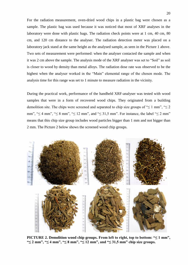
demolition site. The chips were screened and separated to chip size groups of “≤ 1 mm”, “≤ 2
mm”, “≤ 4 mm”, “≤ 8 mm”, “≤ 12 mm”, and “≤ 31,5 mm”. For instance, the label “≤ 2 mm”
means that this chip size group includes wood particles bigger than 1 mm and not bigger than
2 mm. The Picture 2 below shows the screened wood chip groups.
PICTURE 2. Demolition wood chip groups. From left to right, top to bottom: “≤ 1 mm”,
“≤ 2 mm”, “≤ 4 mm”, “≤ 8 mm”, “≤ 12 mm”, and “≤ 31,5 mm” chip size groups.
21
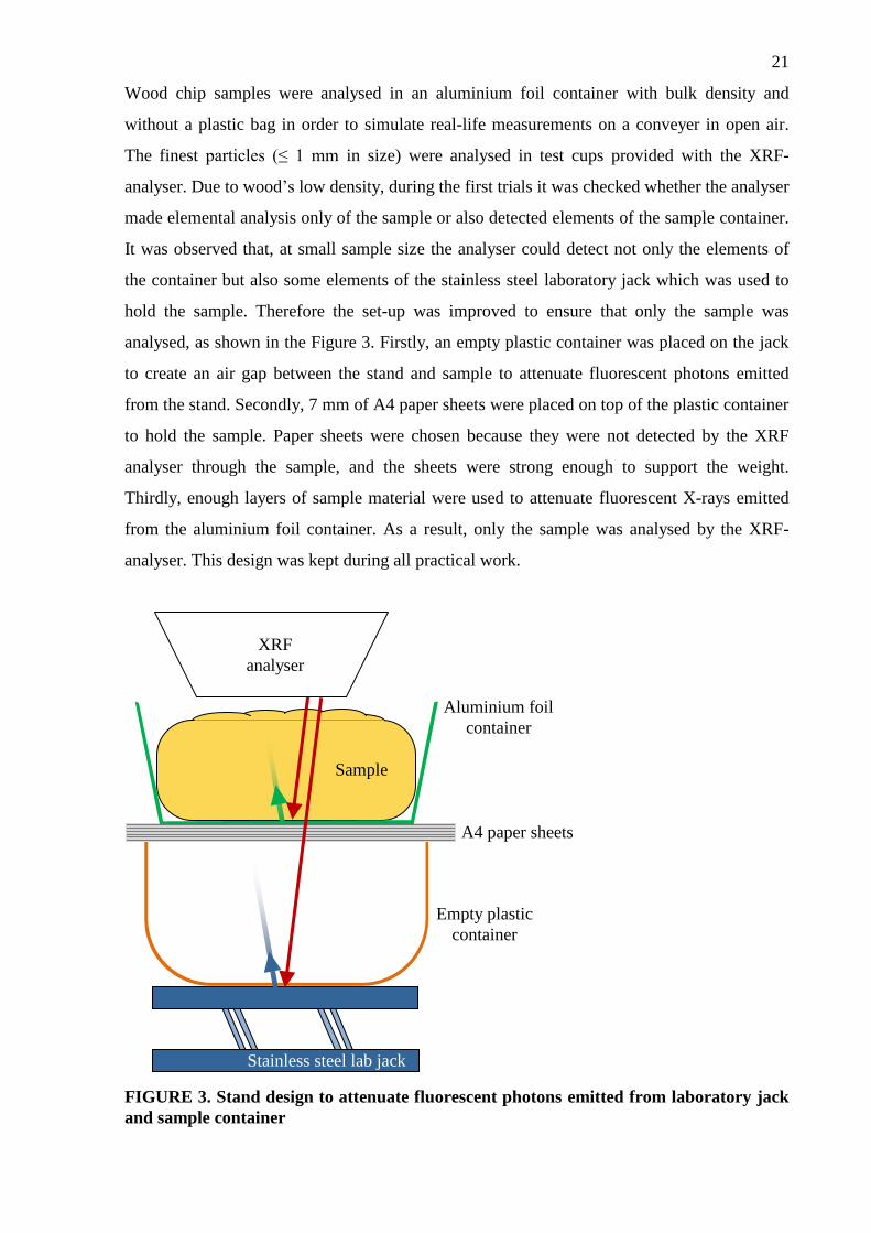
Wood chip samples were analysed in an aluminium foil container with bulk density and
without a plastic bag in order to simulate real-life measurements on a conveyer in open air.
The finest particles (≤ 1 mm in size) were analysed in test cups provided with the XRF-
analyser. Due to wood’s low density, during the first trials it was checked whether the analyser
made elemental analysis only of the sample or also detected elements of the sample container.
It was observed that, at small sample size the analyser could detect not only the elements of
the container but also some elements of the stainless steel laboratory jack which was used to
hold the sample. Therefore the set-up was improved to ensure that only the sample was
analysed, as shown in the Figure 3. Firstly, an empty plastic container was placed on the jack
to create an air gap between the stand and sample to attenuate fluorescent photons emitted
from the stand. Secondly, 7 mm of A4 paper sheets were placed on top of the plastic container
to hold the sample. Paper sheets were chosen because they were not detected by the XRF
analyser through the sample, and the sheets were strong enough to support the weight.
Thirdly, enough layers of sample material were used to attenuate fluorescent X-rays emitted
from the aluminium foil container. As a result, only the sample was analysed by the XRF-
analyser. This design was kept during all practical work.
FIGURE 3. Stand design to attenuate fluorescent photons emitted from laboratory jack
and sample container
Sample
A4 paper sheets
XRF
analyser
Stainless steel lab jack
Aluminium foil
container
Empty plastic
container

22
Another challenging part was to evaluate raw measurement data received from the XRF-
analyser as Microsoft Excel spreadsheet files. The spreadsheet size was too big for convenient
analysis as it had the detected concentration values of 43 elements. Because typically during
the practical work, there were only 10 detected elements of interest for this study, their values
had to be copied from the original Excel file to another file for further analysis. Considering
the fact that manual copying of data was inconvenient, very slow, and it could lead to copying
wrong values, a data copying application was developed within Microsoft Excel in order to
ease working with the raw XRF data. The application interface is shown in the Picture 3
below. This application made 100 % accuracy during the copying, and it dramatically
increased the data processing speed.
PICTURE 3. MS Excel application designed to extract XRF analysis data
With regards to the demolition wood chips, they had a very strong odour and high
concentration of harmful elements. Therefore a breath mask and rubber gloves were worn all
the time, and goggles were additionally used when working with small size particles (“≤ 1
mm”, “≤ 2 mm"). The laboratory room was constantly ventilated during the practical work.
23
The XRF-analyser allowed working in different pre-set testing modes. For this study the mode
“TestAll Geo” was chosen because in this mode the analyser could detect all elements,
including light elements. Other available modes focused on analyses for specific applications,
leaving out several elements from the analysis. The working principle of the analyser was that
it divided all elements into ranges and sequentially measured elements of each range. In the
“TestAll Geo” mode, there were 4 element ranges: light, low, main, and high range. It was
possible to adjust duration of measurement for each range. All element ranges were set to
equal analysis time. For convenience in this study, for example, in figures and tables, the
measurement time corresponds to the analysis time per element range. For instance, a 15
second measurement time is a time that the XRF-analyser needs to analyse a range. In this
case the total measurement time needed to analyse all elements is 15 seconds x 4 ranges = 60
seconds. The analyser took about 0,25 second to switch between the ranges.
With regards to limitations of this study, the most important one is that there were no other
means of checking elemental concentrations found with the XRF analysis. However, the
analyser was periodically controlled with a Standard Reference Material 2709a available from
the US National Institute of Standards and Technology. This standard was dry soil, and all the
control tests were within the standard deviation range given by the manufacturer. Therefore, it
is confident to say that XRF analysis performed on recovered wood samples is accurate. The
latest factory quality control of the analyser prior this study was performed on 11 November
2014.

24
6 PRACTICAL TEST RESULTS
In the tables below the results are expressed in ppm (parts per million). An empty cell means
that an element was not detected by the XRF-analyser. The colours indicate an elemental
concentration, where red colour is the highest value and green colour is the lowest value.
Other colours highlight concentration values between the highest and lowest values.
The XRF analysis results are given with a measurement error, which is two standard
deviations, also known as two-sigma. The result with this error is at around 95 % confidence
level. It means that, for instance, if a concentration of Cl was measured to be 1500 ppm with
the two-sigma error of ±30 ppm, there is a 95 % probability that the true Cl concentration
value is between 1470 ppm and 1530 ppm. All XRF measurements errors in this study
correspond to the two-sigma error. (Thermo Fisher Scientific Inc 2010.)
6.1 Particle size and chemical composition
Around 0,5 kg of sample were screened during 5 minutes for size distribution. This sample
material was used for all following XRF-analyses. The results are presented in the Figure 4.
The most common chip size is between 8 mm and 12 mm accounting for around 23 % of wet
weight. The moisture content of the whole batch was 16,3 %.
16,0
9,4
13,6
23,2
17,5
11,3
4,44,60
5
10
15
20
25
≤31,5≤20≤16≤12≤8≤4≤2≤1
Sh
are
, %
Particle size, mm
FIGURE 4. Particle size distribution of recovered wood sample by wet weight
For XRF analyses, all particles over 12 mm were combined together to form a group ≤ 31,5
mm. Totally, there were 6 size groups. The Table 12 shows the bulk density of each group,
and moisture of selected groups. The “original mix” corresponds to the unsorted raw sample.
The particles with the highest bulk density were the finest particles (≤ 1 mm).
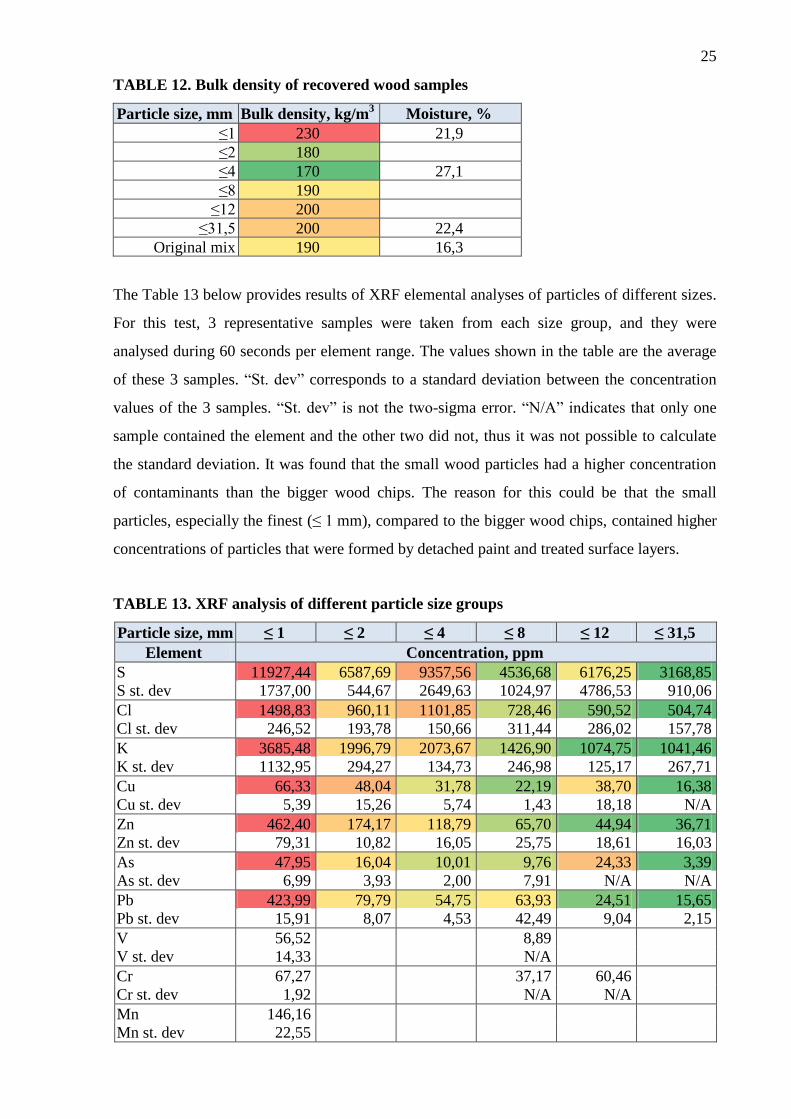
25
TABLE 12. Bulk density of recovered wood samples
Particle size, mm Bulk density, kg/m3 Moisture, %
≤1 230 21,9
≤2 180
≤4 170 27,1
≤8 190
≤12 200
≤31,5 200 22,4
Original mix 190 16,3
The Table 13 below provides results of XRF elemental analyses of particles of different sizes.
For this test, 3 representative samples were taken from each size group, and they were
analysed during 60 seconds per element range. The values shown in the table are the average
of these 3 samples. “St. dev” corresponds to a standard deviation between the concentration
values of the 3 samples. “St. dev” is not the two-sigma error. “N/A” indicates that only one
sample contained the element and the other two did not, thus it was not possible to calculate
the standard deviation. It was found that the small wood particles had a higher concentration
of contaminants than the bigger wood chips. The reason for this could be that the small
particles, especially the finest (≤ 1 mm), compared to the bigger wood chips, contained higher
concentrations of particles that were formed by detached paint and treated surface layers.
TABLE 13. XRF analysis of different particle size groups
Particle size, mm ≤ 1 ≤ 2 ≤ 4 ≤ 8 ≤ 12 ≤ 31,5
Element Concentration, ppm
S 11927,44 6587,69 9357,56 4536,68 6176,25 3168,85
S st. dev 1737,00 544,67 2649,63 1024,97 4786,53 910,06
Cl 1498,83 960,11 1101,85 728,46 590,52 504,74
Cl st. dev 246,52 193,78 150,66 311,44 286,02 157,78
K 3685,48 1996,79 2073,67 1426,90 1074,75 1041,46
K st. dev 1132,95 294,27 134,73 246,98 125,17 267,71
Cu 66,33 48,04 31,78 22,19 38,70 16,38
Cu st. dev 5,39 15,26 5,74 1,43 18,18 N/A
Zn 462,40 174,17 118,79 65,70 44,94 36,71
Zn st. dev 79,31 10,82 16,05 25,75 18,61 16,03
As 47,95 16,04 10,01 9,76 24,33 3,39
As st. dev 6,99 3,93 2,00 7,91 N/A N/A
Pb 423,99 79,79 54,75 63,93 24,51 15,65
Pb st. dev 15,91 8,07 4,53 42,49 9,04 2,15
V 56,52 8,89
V st. dev 14,33 N/A
Cr 67,27 37,17 60,46
Cr st. dev 1,92 N/A N/A
Mn 146,16
Mn st. dev 22,55
26
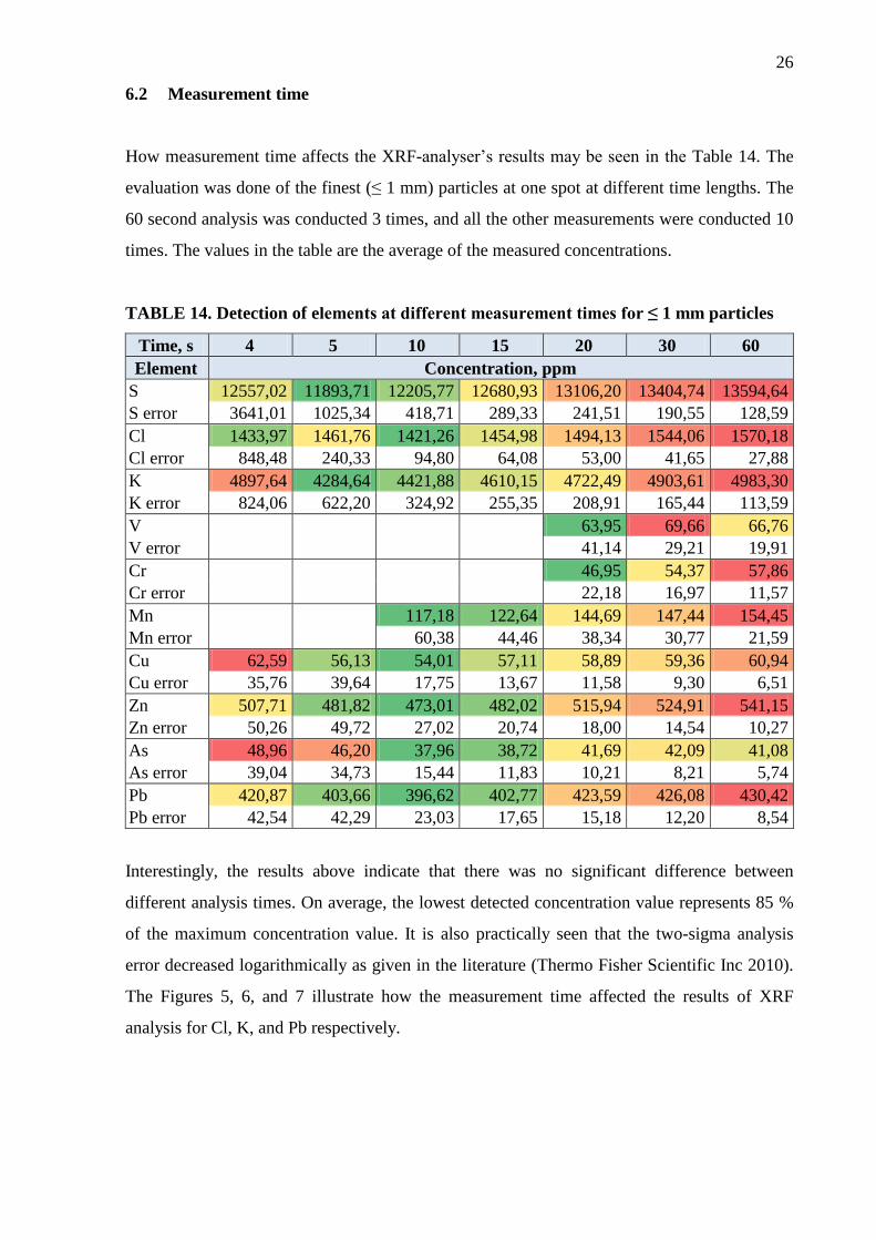
6.2 Measurement time
How measurement time affects the XRF-analyser’s results may be seen in the Table 14. The
evaluation was done of the finest (≤ 1 mm) particles at one spot at different time lengths. The
60 second analysis was conducted 3 times, and all the other measurements were conducted 10
times. The values in the table are the average of the measured concentrations.
TABLE 14. Detection of elements at different measurement times for ≤ 1 mm particles
Time, s 4 5 10 15 20 30 60
Element Concentration, ppm
S 12557,02 11893,71 12205,77 12680,93 13106,20 13404,74 13594,64
S error 3641,01 1025,34 418,71 289,33 241,51 190,55 128,59
Cl 1433,97 1461,76 1421,26 1454,98 1494,13 1544,06 1570,18
Cl error 848,48 240,33 94,80 64,08 53,00 41,65 27,88
K 4897,64 4284,64 4421,88 4610,15 4722,49 4903,61 4983,30
K error 824,06 622,20 324,92 255,35 208,91 165,44 113,59
V 63,95 69,66 66,76
V error 41,14 29,21 19,91
Cr 46,95 54,37 57,86
Cr error 22,18 16,97 11,57
Mn 117,18 122,64 144,69 147,44 154,45
Mn error 60,38 44,46 38,34 30,77 21,59
Cu 62,59 56,13 54,01 57,11 58,89 59,36 60,94
Cu error 35,76 39,64 17,75 13,67 11,58 9,30 6,51
Zn 507,71 481,82 473,01 482,02 515,94 524,91 541,15
Zn error 50,26 49,72 27,02 20,74 18,00 14,54 10,27
As 48,96 46,20 37,96 38,72 41,69 42,09 41,08
As error 39,04 34,73 15,44 11,83 10,21 8,21 5,74
Pb 420,87 403,66 396,62 402,77 423,59 426,08 430,42
Pb error 42,54 42,29 23,03 17,65 15,18 12,20 8,54
Interestingly, the results above indicate that there was no significant difference between
different analysis times. On average, the lowest detected concentration value represents 85 %
of the maximum concentration value. It is also practically seen that the two-sigma analysis
error decreased logarithmically as given in the literature (Thermo Fisher Scientific Inc 2010).
The Figures 5, 6, and 7 illustrate how the measurement time affected the results of XRF
analysis for Cl, K, and Pb respectively.
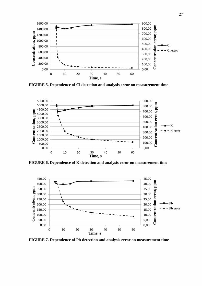
27
0,00
100,00
200,00
300,00
400,00
500,00
600,00
700,00
800,00
900,00
0,00
200,00
400,00
600,00
800,00
1000,00
1200,00
1400,00
1600,00
0 10 20 30 40 50 60
Co
nce
ntr
ati
on
err
or,
pp
m
Co
nce
ntr
ati
on
, p
pm
Time, s
Cl
Cl error
FIGURE 5. Dependence of Cl detection and analysis error on measurement time
0,00
100,00
200,00
300,00
400,00
500,00
600,00
700,00
800,00
900,00
0,00
500,00
1000,00
1500,00
2000,00
2500,00
3000,00
3500,00
4000,00
4500,00
5000,00
5500,00
0 10 20 30 40 50 60C
on
cen
tra
tio
n e
rro
r, p
pm
Co
nce
ntr
ati
on
, p
pm
Time, s
K
K error
FIGURE 6. Dependence of K detection and analysis error on measurement time
0,00
5,00
10,00
15,00
20,00
25,00
30,00
35,00
40,00
45,00
0,00
50,00
100,00
150,00
200,00
250,00
300,00
350,00
400,00
450,00
0 10 20 30 40 50 60
Co
nce
ntr
ati
on
err
or,
pp
m
Co
nce
ntr
ati
on
, p
pm
Time, s
Pb
Pb error
FIGURE 7. Dependence of Pb detection and analysis error on measurement time
28
6.3 Measurement distance
The depths of analysis in recovered wood (for ≤ 12 mm particles) at different distances above
a sample are summarised in the Table 15. It was found using a plastic bag filled with pure iron
powder under the recovered wood sample. Multiple 15 second measurements were carried out
in order to identify Fe at a contact with the sample, at 1 cm and 2 cm above it. Wood particles
were added to increase the analysis depth if Fe was still identified during the measurements.
TABLE 15. Depth of XRF analysis of Fe at different distances to sample
Air gap, mm Analysis depth, mm
0 25
10 20
20 15
For an online XRF measurement system over a belt, it is necessary to have a distance between
the analyser and moving materials. Therefore, an influence of an air gap between the XRF-
analyser and a sample (the ≤ 4 mm particles) was studied. The same spot was tested 4 times at
different time durations and distances. The average values are available in the Table 16 below.
TABLE 16. Detection of elements at different measurement distances to sample and
analysis times, for ≤ 4 mm particles
Time, s 5 s 10 s 15 s
Air gap 0 mm 10 mm 20 mm 0 mm 10 mm 20 mm 0 mm 10 mm 20 mm
Element Concentration, ppm
S 2308,20 1437,42 511,34 6595,26 642,26 399,75 6902,11 618,69 455,22
S error 894,95 539,83 227,32 338,78 194,76 122,97 254,56 137,21 98,51
Cl 1721,95
1387,04 671,86 1447,77 669,91
Cl error 2129,69 103,29 1491,05 76,98 2137,95
K 2617,34 937,21 745,43 2768,71 1030,57 720,73 2868,25 982,25 764,98
K error 382,74 166,08 110,67 230,48 94,93 65,00 163,24 66,76 50,60
Zn 121,11 83,63 128,04 73,96 125,52 78,41
Zn error 33,11 70,45 17,79 32,55 13,26 23,79
Pb 53,45 56,86 54,19 59,00 54,03 53,03 48,87
Pb error 19,13 29,67 10,15 20,96 7,62 14,86 24,09
Cu
44,30
42,58
Cu error 20,37 15,24
As 10,67
As error 6,22
V
V error
Cr 20,71 20,20 16,72 20,29
Cr error 10,44 6,18 7,41 4,68
29
(continues)
TABLE 16. Detection of elements at different measurement distances to sample and
times for ≤ 4 mm particles (continues)
Time, s 20 s 30 s 60 s
Air gap 0 mm 10 mm 20 mm 0 mm 10 mm 20 mm 0 mm 10 mm 20 mm
Element Concentration, ppm
S 6890,40 613,91 373,46 7681,12 645,04 417,29 7234,20 634,83 435,52
S error 212,18 114,82 79,22 164,38 92,05 65,72 106,55 62,36 45,25
Cl 1467,25 703,87 1633,80 661,29 1541,81 722,37
Cl error 64,54 1591,83 49,04 1995,27 32,06 1242,60
K 2956,30 1002,04 787,10 3412,40 1009,71 782,36 3150,55 1012,00 747,08
K error 137,28 56,33 44,68 112,66 44,51 35,33 76,48 30,35 23,42
Zn 136,97 80,49 71,80 139,80 91,16 66,73 134,32 89,94 61,74
Zn error 11,22 20,53 37,77 9,31 17,10 17,66 5,99 11,48 20,36
Pb 57,21 62,00 54,54 56,84 59,75 66,73 55,08 60,09 68,03
Pb error 6,37 13,42 21,58 5,22 10,58 17,66 3,39 7,16 12,54
Cu 37,79
35,95
36,92
Cu error 12,27 10,06 6,59
As 10,95 13,39 12,53
As error 5,19 4,32 2,79
V 5,04 6,12 5,61
V error 2,57 2,97 1,76
Cr 15,05 23,02 17,14 22,07 16,47 22,10
Cr error 6,18 4,16 4,91 3,28 3,33 2,23
In this test, the most accurate result was acquired during a 60 second measurement at a 0 mm
distance to the sample because the analysis error logarithmically decreased with time and
there was no air gap that attenuated fluorescent X-rays. It was not possible to measure above
20 mm because there were not enough counts per second for the XRF-analyser to detect
elements. It produced an error and caused the analyser to stop the tests.
Analysing the above given results, it can be concluded that the air gap changed the detected
elemental concentration very much, especially for light elements. For example, for a 60
second measurement if the XRF-analyser was lifted 10 mm above the sample, it measured S
concentration to be 1/11 of the value acquired during the contact measurement. Cl was not
identified at 20 mm distance at all. However, V and Cr were detected at 10 mm and 20 mm
distances even though the analyser did not identify these elements at the contact measurement.
It probably occurred because at these distances the detection errors were too high and the
analyser misanalysed the concentration of these elements. Elements Cu and As were not
identified at any of the tested air gaps, probably due to their low concentrations.
30
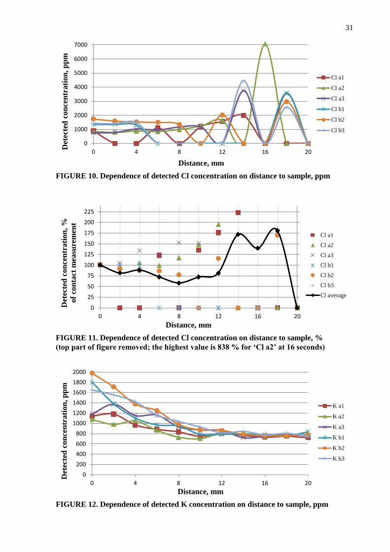
A more extensive testing was conducted in order to find any possible dependence of element
detection on the elevation distance. Two samples were analysed: oven-dried ≤ 8 mm particles,
labelled “a”, and oven-dried 6 mm particles received by grinding the ≤ 31,5 mm particles,
labelled “b”. Three different spots of each sample were analysed, labelling the spots, for
example, as “a1” or “b2”. The XRF-analyser was elevated above the samples with a step of 2
mm. The measurement time was set to 5 seconds per element range. 2 measurements were
taken at each elevation distance, and their average value was used for the calculation. Because
the analysis results were received in ppm, in order to compare all the measurements regardless
of their real elemental concentration and find a possible trend, the data was converted to per
cent. 100 % was set to be the concentration value detected at a 0 mm distance to the wood
samples. The results of data analysis are presented in the following Figures 8 - 24 below.
0
1000
2000
3000
4000
5000
6000
7000
8000
9000
10000
0 4 8 12 16 20
Det
ecte
d c
on
cen
trati
on
, p
pm
Distance, mm
S a1
S a2
S a3
S b1
S b2
S b3
FIGURE 8. Dependence of detected S concentration on distance to sample, ppm
0
20
40
60
80
100
120
0
20
40
60
80
100
120
0 4 8 12 16 20
Det
ecte
d c
on
cen
trati
on
, %
of
con
tact
mea
sure
men
t
Distance, mm
S a1
S a2
S a3
S b1
S b3
S b2
S average
FIGURE 9. Dependence of detected S concentration on distance to sample, %
31
0
1000
2000
3000
4000
5000
6000
7000
0 4 8 12 16 20
Det
ecte
d c
on
cen
trati
on
, p
pm
Distance, mm
Cl a1
Cl a2
Cl a3
Cl b1
Cl b2
Cl b3
FIGURE 10. Dependence of detected Cl concentration on distance to sample, ppm
0
25
50
75
100
125
150
175
200
225
0
25
50
75
100
125
150
175
200
225
0 4 8 12 16 20
Det
ecte
d c
on
cen
trati
on
, %
of
con
tact
mea
sure
men
t
Distance, mm
Cl a1
Cl a2
Cl a3
Cl b1
Cl b2
Cl b3
Cl average
FIGURE 11. Dependence of detected Cl concentration on distance to sample, %
(top part of figure removed; the highest value is 838 % for ‘Cl a2’ at 16 seconds)
0
200
400
600
800
1000
1200
1400
1600
1800
2000
0 4 8 12 16 20
Det
ecte
d c
on
cen
trati
on
, p
pm
Distance, mm
K a1
K a2
K a3
K b1
K b2
K b3
FIGURE 12. Dependence of detected K concentration on distance to sample, ppm

32
0
20
40
60
80
100
120
0
20
40
60
80
100
120
0 4 8 12 16 20
Det
ecte
d c
on
cen
trati
on
, %
of
con
tact
mea
sure
men
t
Distance, mm
K a1
K a2
K a3
K b1
K b2
K b3
K average
FIGURE 13. Dependence of detected K concentration on distance to sample, %
0
40
80
120
160
200
240
280
320
360
400
440
0 4 8 12 16 20
Det
ecte
d c
on
cen
trati
on
, p
pm
Distance, mm
Cu a1
Cu a2
Cu a3
FIGURE 14. Dependence of detected Cu concentration on distance to sample, ppm
0
20
40
60
80
100
120
0
20
40
60
80
100
120
0 4 8 12 16 20
Det
ecte
d c
on
cen
trati
on
, %
of
con
tact
mea
sure
men
t
Distance, mm
Cu a1
Cu a2
Cu a3
Cu average
FIGURE 15. Dependence of detected Cu concentration on distance to sample, %

33
0
20
40
60
80
100
120
140
160
180
200
220
0 4 8 12 16 20
Det
ecte
d c
on
cen
trati
on
, p
pm
Distance, mm
Zn a1
Zn a2
Zn a3
Zn b1
Zn b2
Zn b3
FIGURE 16. Dependence of detected Zn concentration on distance to sample, ppm
0
20
40
60
80
100
120
140
0
20
40
60
80
100
120
140
0 4 8 12 16 20
Det
ecte
d c
on
cen
trati
on
, %
of
con
tact
mea
sure
men
t
Distance, mm
Zn a1
Zn a2
Zn a3
Zn b1
Zn b2
Zn b3
Zn average
FIGURE 17. Dependence of detected Zn concentration on distance to sample, %
0
25
50
75
100
125
150
175
200
225
250
275
300
0 4 8 12 16 20
Det
ecte
d c
on
cen
trati
on
, p
pm
Distance, mm
As a1
As a2
As a3
FIGURE 18. Dependence of detected As concentration on distance to sample, ppm
34
0
20
40
60
80
100
120
140
160
180
200
0
20
40
60
80
100
120
140
160
180
200
0 4 8 12 16 20
Det
ecte
d c
on
cen
trati
on
, %
of
con
tact
mea
sure
men
t
Distance, mm
As a1
As a2
As a3
As average
FIGURE 19. Dependence of detected As concentration on distance to sample, %
0
20
40
60
80
100
120
140
160
180
0 4 8 12 16 20
Det
ecte
d c
on
cen
trati
on
, p
pm
Distance, mm
Pb a2
Pb a3
Pb b1
Pb b2
Pb b3
FIGURE 20. Dependence of detected Pb concentration on distance to sample, ppm
0
25
50
75
100
125
150
175
200
225
0
25
50
75
100
125
150
175
200
225
0 4 8 12 16 20
Det
ecte
d c
on
cen
trati
on
, %
of
con
tact
mea
sure
men
t
Distance, mm
Pb a2
Pb a3
Pb b1
Pb b2
Pb b3
Pb average
FIGURE 21. Dependence of detected Pb concentration on distance to sample, %

35
0
75
150
225
300
375
450
525
600
675
750
0 4 8 12 16 20
Det
ecte
d c
on
cen
trati
on
, p
pm
Distance, mm
Cr a1
Cr a2
Cr a3
FIGURE 22. Dependence of detected Cr concentration on distance to sample, ppm
0
20
40
60
80
100
120
0
20
40
60
80
100
120
0 4 8 12 16 20
Det
ecte
d c
on
cen
trati
on
, %
of
con
tact
mea
sure
men
t
Distance, mm
Cr a1
Cr a2
Cr a3
Cr average
FIGURE 23. Dependence of detected Cr concentration on distance to sample, %
y = -3,0195x + 99,347R² = 0,903
0
10
20
30
40
50
60
70
80
90
100
0 4 8 12 16 20
Det
ecte
d c
on
cen
trati
on
, %
of
con
tact
mea
sure
men
t
Distance, mm
Average of all presented
elements
Linear (Average of all
presented elements)
FIGURE 24. Dependence of detected elemental concentration on distance to sample,
average of all presented elements (S, Cl, K, Cu, Zn, As, Pb, Cr)

36
Analysing the Figures 8 – 23 presented above, it can be seen that as a general trend, the
detected concentrations fluctuated considerably between the measurements of same elements.
The variations increased with increasing distance, especially above 6 mm. However, K and Cr
had smooth trend lines. For As and Pb, at low original concentration value (at 0 mm distance)
the detected concentrations increased with increasing distance; however at high original
concentration values, their detected concentrations decreased with increasing distance. The
average trend of all presented elements is illustrated in the Figure 24. It indicates that,
generally from 0 mm to 12 mm, detected concentrations were proportional to the distance.
However, detection of elements at a distance greater than 12 mm did not follow the trend.
FIGURE 25. XRF analysis at different distances to sample
The observed fluctuations in the detected concentration values may be explained by several
mechanisms that occurred during the conducted tests. Firstly, the increased air gap attenuated
fluorescent photons, and it led to a reduced number of counts per second on the XRF detector,
and thus, the detected concentrations. Secondly, compared to long analysis time, the short
measurement time used in these tests produced greater errors. Moreover, even those
concentration values received from the measurements taken for 5 seconds at the same distance
sometimes differed considerably. Thirdly, because the demolition wood samples were highly
heterogeneous, when the analyser was moved vertically, its primary X-ray beam could analyse
a different particle inside the sample, as schematically shown in the Figure 25 above. Due to
the fact that the X-ray source tube is fixed at an angel inside the analyser, moving the analyser
vertically created a small displacement at the horizontal level of the initial measurement.
Sample
XRF
analyser
Sample
XRF
analyser
37
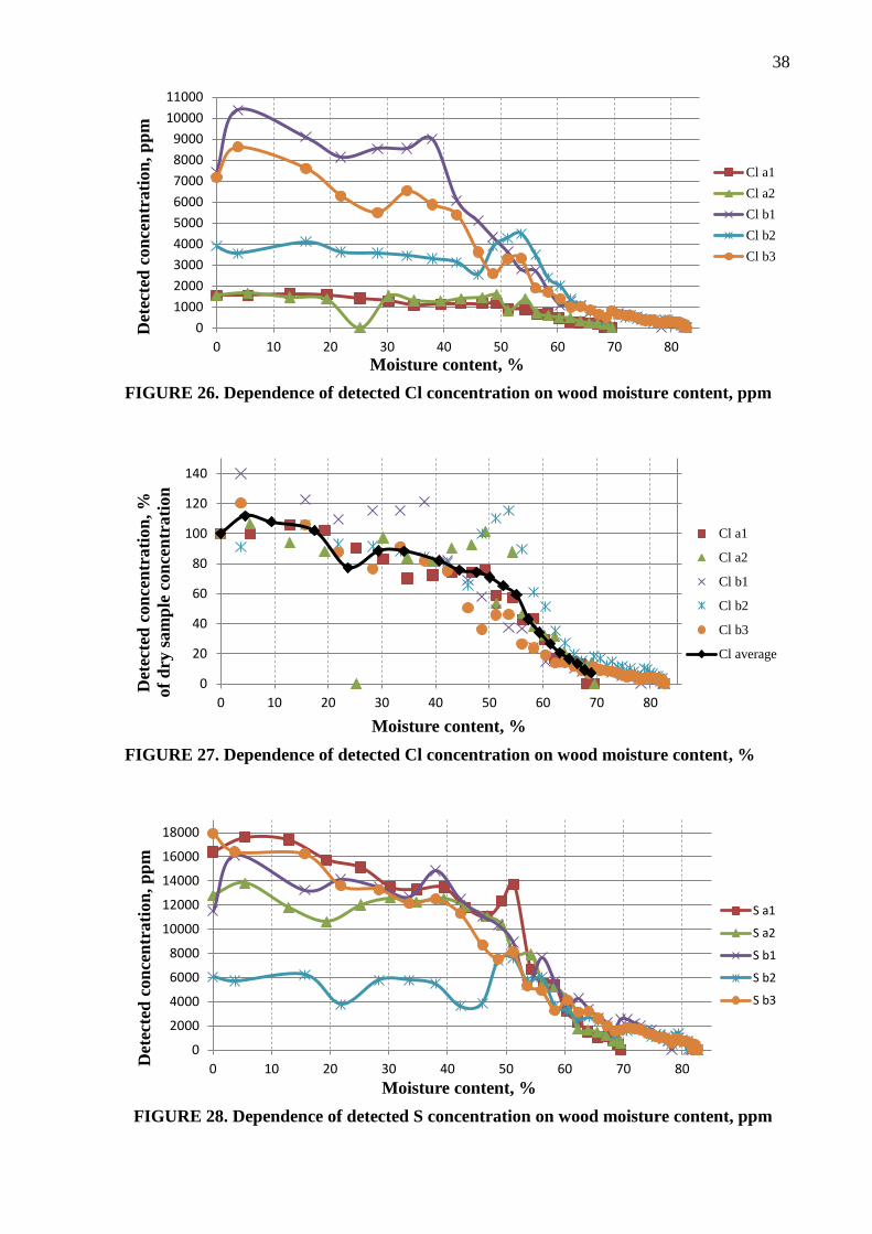
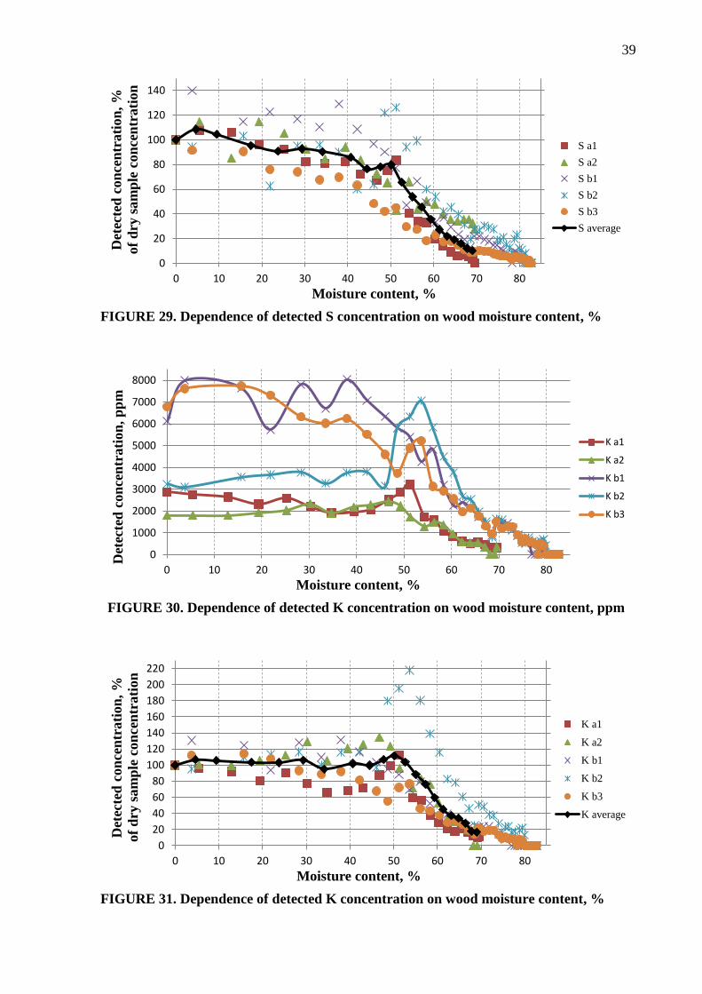
6.4 Wood moisture
The aim of this test was to find out if there was any possible correlation between the measured
and real elemental concentrations in recovered wood and observe at what wood moisture
levels the XRF-analyser stopped identifying elements. Two recovered wood samples of
roughly 50 grams (dry mass) were prepared and soaked in distilled water for 10 days. The first
sample labelled “a” was the ≤ 8 mm particles, and the second sample labelled “b” was the ≤
31,5 mm particles grinded to particles of 6 mm in size. The moisture contents in the samples
were raised to around 70 % and 80 % for the sample “a” and “b” respectively. The samples
were dried in an oven at 105 °C and periodically taken for the XRF analysis.
Different spots (a1, a2, b1, b2, b3) of the samples were analysed during 5 seconds per element
range. Two XRF measurements were taken per a spot. The samples were weighed before the
XRF analysis and immediately after it. The average of these two mass values was used for
calculating the moisture content. On average, 1 g of water evaporated during the analyses. A
paper sheet with marked coordinates of the spots was used in order to constantly place the
XRF-analyser above the spots.
The detected elemental concentrations were in ppm. However, the concentrations varied
between the samples and spots considerably, as the example of Cl shows in the Figure 26
below. Because the aim of the test was to evaluate how moisture affected the XRF readings,
all result values were converted to per cents of the measured concentration at 0 % moisture
content. Therefore the detected elemental concentration at the 0 % moisture level was set to a
100 % elemental concentration, and the other measured elemental concentrations at different
moisture levels were calculated as proportions to it.
This data presentation method allows easier comparison of the results regardless of their
actual concentrations. For instance, the Figure 27 represents the same Cl values as the Figure
26 but in percentage. As a result, the relationship between the detected Cl concentration and
the wood moisture content can be clearly seen regardless of the measured concentrations.
Such a representation also helped to create the average dependence across all the XRF
element measurements using statistical methods. The average trend was calculated up to 70 %
of moisture level as it was the highest common moisture value for the samples “a” and “b”.
38
0
1000
2000
3000
4000
5000
6000
7000
8000
9000
10000
11000
0 10 20 30 40 50 60 70 80
Det
ecte
d c
on
cen
tra
tio
n,
pp
m
Moisture content, %
Cl a1
Cl a2
Cl b1
Cl b2
Cl b3
FIGURE 26. Dependence of detected Cl concentration on wood moisture content, ppm
0
20
40
60
80
100
120
140
0
20
40
60
80
100
120
140
0 10 20 30 40 50 60 70 80
Det
ecte
d c
on
cen
trati
on
, %
of
dry
sam
ple
con
cen
trati
on
Moisture content, %
Cl a1
Cl a2
Cl b1
Cl b2
Cl b3
Cl average
FIGURE 27. Dependence of detected Cl concentration on wood moisture content, %
0
2000
4000
6000
8000
10000
12000
14000
16000
18000
0 10 20 30 40 50 60 70 80Det
ecte
d c
on
cen
tra
tio
n,
pp
m
Moisture content, %
S a1
S a2
S b1
S b2
S b3
FIGURE 28. Dependence of detected S concentration on wood moisture content, ppm
39
0
20
40
60
80
100
120
140
0
20
40
60
80
100
120
140
0 10 20 30 40 50 60 70 80
Det
ecte
d c
on
cen
tra
tio
n,
%
of
dry
sa
mp
le c
on
cen
tra
tio
n
Moisture content, %
S a1
S a2
S b1
S b2
S b3
S average
FIGURE 29. Dependence of detected S concentration on wood moisture content, %
0
1000
2000
3000
4000
5000
6000
7000
8000
0 10 20 30 40 50 60 70 80
Det
ecte
d c
on
cen
tra
tio
n,
pp
m
Moisture content, %
K a1
K a2
K b1
K b2
K b3
FIGURE 30. Dependence of detected K concentration on wood moisture content, ppm
0
20
40
60
80
100
120
140
160
180
200
220
0
20
40
60
80
100
120
140
160
180
200
220
0 10 20 30 40 50 60 70 80
Det
ecte
d c
on
cen
tra
tio
n,
%
of
dry
sa
mp
le c
on
cen
tra
tio
n
Moisture content, %
K a1
K a2
K b1
K b2
K b3
K average
FIGURE 31. Dependence of detected K concentration on wood moisture content, %
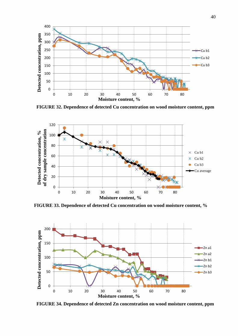
40
0
50
100
150
200
250
300
350
400
0 10 20 30 40 50 60 70 80
Det
ecte
d c
on
cen
tra
tio
n,
pp
m
Moisture content, %
Cu b1
Cu b2
Cu b3
FIGURE 32. Dependence of detected Cu concentration on wood moisture content, ppm
0
20
40
60
80
100
120
0
20
40
60
80
100
120
0 10 20 30 40 50 60 70 80
Det
ecte
d c
on
cen
tra
tio
n,
%
of
dry
sa
mp
le c
on
cen
tra
tio
n
Moisture content, %
Cu b1
Cu b2
Cu b3
Cu average
FIGURE 33. Dependence of detected Cu concentration on wood moisture content, %
0
50
100
150
200
0 10 20 30 40 50 60 70 80
Det
ecte
d c
on
cen
tra
tio
n,
pp
m
Moisture content, %
Zn a1
Zn a2
Zn b1
Zn b2
Zn b3
FIGURE 34. Dependence of detected Zn concentration on wood moisture content, ppm

41
0
20
40
60
80
100
120
0
20
40
60
80
100
120
0 10 20 30 40 50 60 70 80
Det
ecte
d c
on
cen
tra
tio
n,
%
of
dry
sa
mp
le c
on
cen
tra
tio
n
Moisture content, %
Zn a1
Zn a2
Zn b1
Zn b2
Zn b3
Zn average
FIGURE 35. Dependence of detected Zn concentration on wood moisture content, %
0
50
100
150
200
250
300
350
400
450
0 10 20 30 40 50 60 70 80
Det
ecte
d c
on
cen
tra
tio
n,
pp
m
Moisture content, %
As b1
As b2
As b3
FIGURE 36. Dependence of detected As concentration on wood moisture content, ppm
0
20
40
60
80
100
120
0
20
40
60
80
100
120
0 10 20 30 40 50 60 70 80
Det
ecte
d c
on
cen
tra
tio
n,
%
of
dry
sa
mp
le c
on
cen
tra
tio
n
Moisture content, %
As b1
As b2
As b3
As average
FIGURE 37. Dependence of detected As concentration on wood moisture content, %

42
0
20
40
60
80
100
120
0 10 20 30 40 50 60 70 80
Det
ecte
d c
on
cen
tra
tio
n,
pp
m
Moisture content, %
Pb a1
Pb a2
Pb b1
Pb b2
Pb b3
FIGURE 38. Dependence of detected Pb concentration on wood moisture content, ppm
0
20
40
60
80
100
120
140
0
20
40
60
80
100
120
140
0 10 20 30 40 50 60 70 80
Det
ecte
d c
on
cen
tra
tio
n,
%
of
dry
sa
mp
le c
on
cen
tra
tio
n
Moisture content, %
Pb a1
Pb a2
Pb b1
Pb b2
Pb b3
Pb average
FIGURE 39. Dependence of detected Pb concentration on wood moisture content, %
0
100
200
300
400
500
600
700
800
0 10 20 30 40 50 60 70 80
Det
ecte
d c
on
cen
trati
on
, p
pm
Moisture content, %
Cr b1
Cr b2
FIGURE 40. Dependence of detected Cr concentration on wood moisture content, ppm
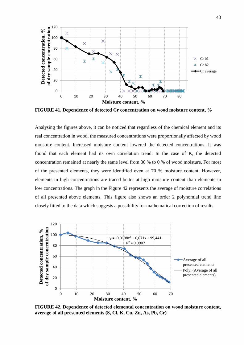
43
0
20
40
60
80
100
120
0
20
40
60
80
100
120
0 10 20 30 40 50 60 70 80
Det
ecte
d c
on
cen
trati
on
, %
of
dry
sam
ple
con
cen
trati
on
Moisture content, %
Cr b1
Cr b2
Cr average
FIGURE 41. Dependence of detected Cr concentration on wood moisture content, %
Analysing the figures above, it can be noticed that regardless of the chemical element and its
real concentration in wood, the measured concentrations were proportionally affected by wood
moisture content. Increased moisture content lowered the detected concentrations. It was
found that each element had its own correlation trend. In the case of K, the detected
concentration remained at nearly the same level from 30 % to 0 % of wood moisture. For most
of the presented elements, they were identified even at 70 % moisture content. However,
elements in high concentrations are traced better at high moisture content than elements in
low concentrations. The graph in the Figure 42 represents the average of moisture correlations
of all presented above elements. This figure also shows an order 2 polynomial trend line
closely fitted to the data which suggests a possibility for mathematical correction of results.
y = -0,0198x2 + 0,071x + 99,441R² = 0,9907
0
20
40
60
80
100
120
0 10 20 30 40 50 60 70
Det
ecte
d c
on
cen
trati
on
, %
of
dry
sam
ple
con
cen
trati
on
Moisture content, %
Average of all
presented elements
Poly. (Average of all
presented elements)
FIGURE 42. Dependence of detected elemental concentration on wood moisture content,
average of all presented elements (S, Cl, K, Cu, Zn, As, Pb, Cr)
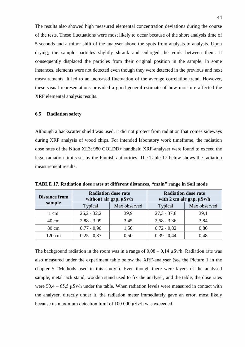
44
The results also showed high measured elemental concentration deviations during the course
of the tests. These fluctuations were most likely to occur because of the short analysis time of
5 seconds and a minor shift of the analyser above the spots from analysis to analysis. Upon
drying, the sample particles slightly shrank and enlarged the voids between them. It
consequently displaced the particles from their original position in the sample. In some
instances, elements were not detected even though they were detected in the previous and next
measurements. It led to an increased fluctuation of the average correlation trend. However,
these visual representations provided a good general estimate of how moisture affected the
XRF elemental analysis results.
6.5 Radiation safety
Although a backscatter shield was used, it did not protect from radiation that comes sideways
during XRF analysis of wood chips. For intended laboratory work timeframe, the radiation
dose rates of the Niton XL3t 980 GOLDD+ handheld XRF-analyser were found to exceed the
legal radiation limits set by the Finnish authorities. The Table 17 below shows the radiation
measurement results.
TABLE 17. Radiation dose rates at different distances, “main” range in Soil mode
Distance from
sample
Radiation dose rate
without air gap, µSv/h
Radiation dose rate
with 2 cm air gap, µSv/h
Typical Max observed Typical Max observed
1 cm 26,2 - 32,2 39,9 27,3 - 37,8 39,1
40 cm 2,88 - 3,09 3,45 2,58 - 3,36 3,84
80 cm 0,77 - 0,90 1,50 0,72 - 0,82 0,86
120 cm 0,25 - 0,37 0,50 0,39 - 0,44 0,48
The background radiation in the room was in a range of 0,08 – 0,14 µSv/h. Radiation rate was
also measured under the experiment table below the XRF-analyser (see the Picture 1 in the
chapter 5 “Methods used in this study”). Even though there were layers of the analysed
sample, metal jack stand, wooden stand used to fix the analyser, and the table, the dose rates
were 50,4 – 65,5 µSv/h under the table. When radiation levels were measured in contact with
the analyser, directly under it, the radiation meter immediately gave an error, most likely
because its maximum detection limit of 100 000 µSv/h was exceeded.

45
PICTURE 4. Experimental set-up for XRF-analyser with lead shielding
In order to illuminate the unwanted radiation which was scattered from samples during
analyses, the test equipment was shielded with several 2 mm lead plates as seen in the Picture
4 above. As a result, the radiation was completely absorbed, and at any distance from the
shielding the radiation meter showed only the background radiation dose. This set-up was
used for all measurements of recovered wood samples.
46
7 CONCLUSIONS
The results of the practical tests during this thesis project showed consistency with previous
studies on XRF analysis, particularly, that moisture, air gap and short measurement time
negatively affected the detected elemental concentrations. However, the literature review
provided only general information, for example, that moisture reduced XRF detectability of
elements without any given correlations. This thesis presented valuable and more detailed
information on the limitations of XRF analysis. Moreover, now the data is available for
specific challenging elements in recovered wood fuel.
The literature review and practical work showed that analysis of wood with XRF equipment
was challenging due to its limitations, however it was practically feasible. Understanding of
limiting conditions and their effects on the XRF analysis results should improve accuracy of
solid fuel quality control with a handheld XRF-analyser. Recommendations for better
measurements are provided below. This study was made with a Niton XL3t 980 GOLDD+.
Firstly, the shortest and yet accurate analysis time for wood samples is 30 seconds per element
range, or 2 minutes per full analysis. Secondly, a contact measurement with a sample is most
desirable. Thirdly, wood moisture lowers detected elemental concentrations, however it is
possible to mathematically correct the measured values when knowing the moisture content.
Lastly, it was found that the small recovered wood particles (4 mm and less) contained high
concentrations of contaminating elements. Therefore, it is advisable to illuminate them prior
combustion.
It should be noted that results of XRF analysis represent only a very small part of a sample.
One way to improve the accuracy is to make more measurements. Ultimately, an online XRF
measurement system could be a solution to this issue as it would scan wood chips
continuously on a moving conveyor.
With regards to an online XRF system, it should be able to analyse all ranges of elements,
including light and heavy elements, without the need to switch between the element ranges. It
would increase the processing speed and thus the amount of analysed material on a conveyer.
The XRF detector of the online measurement system should not be located further than 12
mm above the sample as the air gap attenuates XRF photons and drastically reduces the
47
detected elemental concentration. Also, this system should have a cooling system because the
XRF-analyser overheats during long measurements and does not allow working until it has
cooled down.
Lastly, further studies should be organised for more detailed research on XRF performance in
recovered wood quality control. Particularly for an online XRF system, a high number of tests
is needed to create accurate correlation formulas for effects of wood moisture on the XRF
analysis results. Dependence of measured elemental concentrations on elevation distance
above wood samples should be further explored for possible usable correlation formulas.
Finally, performance of the XRF-analyser over moving samples should be studied as a
simulation of a working conveyer belt.
In the conclusion, the studied XRF analyser can be used in solid biofuel quality control. It is
capable of identifying the elements listed in the EU biofuel standards and specifications,
except for N and Na. The XRF analysis is fast and accurate, and its precision can be further
increased with mathematical corrections of negative effects of known limitations. The
elemental XRF analysis with the handheld XRF-analyser can be performed by personnel
without a background in physics or chemistry. However, personal radiation safety must be
ensured when analysing wood samples due to high radiation dose rates near the analyser.
48
REFERENCES
Amptek Inc. What is XRF?. WWW-document. http://www.amptek.com/xrf/. No update
information. Referred 22.4.2015.
Anzelmo, John, Bouchard, Mathieu & Provencher Marie-Eve 2014. X-ray fluorescence
spectroscopy, part II: sample preparation. Spectroscopy magazine. Volume 29 Number 7. PDF
document. http://images2.advanstar.com/PixelMags/spectroscopy/pdf/2014-07.pdf. No update
information. Referred 22.4.2015.
Bankiewicz, Dorota 2012. Corrosion behaviour of boiler tube materials during combustion of
fuels containing Zn and Pb. Academic dissertation. PDF document. https://www.doria.fi/
bitstream/handle/10024/77050/bankiewicz_dorota.pdf?sequence=2. No update information.
Referred 22.4.2015.
Bruker 2008. Draft Bruker XRF spectroscopy user guide: spectral interpretation and sources
of interference. PDF document. http://www.ifuap.buap.mx/Workshop-XRF/XRF-theory/
Bruker_Tracerand_Artax_XRF_Raw_Spectrum_Analysis_User_.pdf. Updated 11.11.2008.
Referred 22.4.2015.
Bruker 2012. EDX vs WDX: Head to Head. PDF document. http://www.bruker.com/
fileadmin/user_upload/8-PDF-Docs/X-rayDiffraction_ElementalAnalysis/XRF/Webinars/
Bruker_AXS_EDX_vs_WDX_Webinar_Slides.pdf. Updated 18.4.2012. Referred 22.4.2015.
Bruker. Periodic table of elements and X-ray energies. PDF document. http://www.bruker
.com/fileadmin/user_upload/8-PDF-Docs/X-rayDiffraction_ElementalAnalysis/HH-XRF
/Misc/Periodic_Table_and_X-ray_Energies.pdf. No update information. Referred 22.4.2015.
European recovered fuel organisation. Information document on EN 15359 “Solid recovered
fuels – specifications and classes”. PDF document. http://erfo.info/fileadmin/user_upload
/erfo/documents/reports/Information_document_EN15359.pdf. No update information.
Referred 22.4.2015.
49
Fellin, Marco, Negri, Martino, Mazzei, Federico & Zanuttini, Roberto 2014. Characterization
of ED-XRF technology applied to wooden matrix. Wood research. PDF document.
http://www.centrumdp.sk/wr/201404/02.pdf. No update information. Referred 22.4.2015.
Finnish radiation and nuclear safety authority 2008. Use of control and analytical X-ray
apparatus. PDF document. http://www.finlex.fi/data/normit/35279-ST5-2e.pdf. No update
information. Referred 22.4.2015.
Glanzman, R. & Closs, L. 2007. Field portable X-ray fluorescence geochemical analysis – its
contribution to onsite real-time project evaluation. PDF document. http://www.dmec.ca/ex07-
dvd/E07/pdfs/15.pdf. No update information. Referred 22.4.2015.
Guthrie, James 2012. Overview of X-ray fluorescence. WWW-document. http://archaeometry.
missouri.edu/xrf_overview.html. Updated 21.11.2014. Referred 22.4.2015.
International renewable energy agency 2014. Global bioenergy: supply and demand
projections. PDF document. http://irena.org/remap/IRENA_REmap_2030_Biomass_
paper_2014.pdf. No update information. Referred 22.4.2015.
ISO 17225-1:2014. Solid biofuels. Fuel specifications and classes. Part 1: general
requirements. International standard.
Jones, Frida 2013. Characterisation of waste for combustion – with special reference to the
role of zinc. Doctoral thesis. PDF document. https://www.doria.fi/bitstream/handle/
10024/93783/jones_frida.pdf?sequence=2. No update information. Referred 22.4.2015.
Merlini, Mattia 2013. Classification and specification of SRF according to EN 15359 and
overview of the European standards developed by CEN/TC 343 “Solid recovered fuels” PDF
document. http://www.ieabioenergytask36.org/vbulletin/attachment.php?attachmentid
=357&d=1385465332. No update information. Referred 22.4.2015.
Nakhaei F., Sam A. & Mosavi MR 2012. Prediction of XRF analyzers error for elements on-
line assaying using Kalman filter. WWW-document. http://www.sciencedirect.com/science
/article/pii/S2095268612001371. No update information. Referred 22.4.2015.

50
PAS 111:2012. Specification for the requirements and test methods for processing waste
wood. Waste and Resources Action Programme. PDF document.
http://www.woodrecyclers.org/PAS111.pdf. No update information. Referred 22.4.2015.
Sandberg, Jan 2011. Fouling in biomass fired boilers. Doctoral thesis. PDF document.
http://www.diva-portal.org/smash/get/diva2:452326/FULLTEXT02. No update information.
Referred 22.4.2015.
Solo-Gabriele, Helena, Townsend, Timothy, Hahn, David, Hosein, Naila, Jacobi, Gary,
Jambeck, Jenna, Moskal, Tom & Kenjiro, Iida 2001. On-line sorting technologies for CCA-
treated wood. PDF document. http://www.dep.state.fl.us/waste/quick_topics/publications
/shw/recycling/InnovativeGrants/IGyear3/finalreports/sarasota.pdf. No update information.
Referred 22.4.2015.
Solo-Gabriele, Helena, Townsend, Timothy, Hahn, David, Moskal, Thomas, Hosein, Naila,
Jambeck, Jenna & Jacobi, Gary 2003. Evaluation of XRF and LIBS technologies for on-line
sorting of CCA-treated wood waste. WWW-document. http://www.sciencedirect.com/science
/article/pii/S0956053X03002058. No update information. Referred 22.4.2015.
Thermo Fisher Scientific Inc 2009. Mining FAQ. PDF document. http://www.us-tech.co.za/
downloads/thermo/Mining%20FAQs%202009Sept.pdf. No update information. Referred
22.4.2015.
Thermo Fisher Scientific Inc 2010. XL3 analyzer. User guide. PDF document. http://www.
tttenviro. com/wp-content/uploads/Manual-XL3-Series-v7.0.11.pdf. No update information.
Referred 22.4.2015.
Thermo Fisher Scientific Inc 2013. XRF technology for non-scientists. PDF document.
http://www.thermoscientific.com/content/dam/tfs/ATG/CAD/CAD%20Marketing%20Materia
l/CAD%20Marketing%20Documents/PAI%20Documents/TS-eBook-XRF-Technology-in-
the-Field.pdf. No update information. Referred 22.4.2015.
Thermo Fisher Scientific Inc 2014. X-ray tube radiation survey certificate.

51
Thermo Fisher Scientific Inc. Thermo Scientific Niton XL3t GOLDD+ Specifications. PDF
document. http://www.niton.com/docs/literature/Niton_XL3t_GOLDD_Spec_Sheet.pdf
?sfvrsn=2. No update information. Referred 22.4.2015.
US Environmental Protection Agency 2004. X-ray fluorescence instruments - frequently asked
questions. PDF document. http://www.epa.gov/superfund/health/contaminants/lead
/products/xrffaqs.pdf. Updated 25.5.2004. Referred 22.4.2015.
Vainikka, Pasi 2011. Occurrence of bromine in fluidised bed combustion of solid recovered
fuel. Academic dissertation. PDF document. http://www2.vtt.fi/inf/pdf/publications
/2011/P778.pdf. No update information. Referred 22.4.2015.
Vakkilainen, Esa, Kuparinen, Katja & Heinimö, Jussi 2013. Large industrial users of energy
biomass. Report for IEA Bioenergy Task 40. PDF document. http://www.bioenergytrade.org/
downloads/t40-large-industrial-biomass-users.pdf. No update information. Referred
22.4.2015.
Valmari, Tuomas 2000. Potassium behaviour during combustion of wood in circulating
fluidised bed power plants. Academic dissertation. PDF document. http://lib.tkk.fi/Diss/2000/
isbn9513855708/isbn9513855708.pdf. No update information. Referred 22.4.2015.
Viklund, Peter 2013. Superheater corrosion in biomass and waste fired boilers.
Characterisation, causes and prevention of chlorine-induced corrosion. Doctoral thesis. PDF
document. http://www.diva-portal.org/smash/get/diva2:614735/INSIDE01.pdf. No update
information. Referred 22.4.2015.
Waste and Resources Action Programme 2009. Automated sorting of treated wood waste.
PDF document. http://www2.wrap. org.uk/downloads/MDD015_Final_Report_
11.03.10.7afca182.9756.pdf. No update information. Referred 22.4.2015.
Wobrauschek, Peter, Streli Christina & Lindgren, Eva Selin 2010. Energy Dispersive, X-ray
Fluorescence Analysis. Encyclopedia of Analytical Chemistry R.A. Meyers. PDF document.
http://publik.tuwien.ac.at/files/PubDat_187656.pdf. No update information. Referred
22.4.2015.


