Download - Bo otstrap - Rice University

Bootstrap Unit Root Tests in Panels
with Cross-Sectional Dependency1
Yoosoon Chang
Department of Economics
Rice University
Abstract
We apply bootstrap methodology to unit root tests for dependent panels with N
cross-sectional units and T time series observations. More speci�cally, we let each
panel be driven by a general linear process which may be di�erent across cross-
sectional units, and approximate it by a �nite order autoregressive integrated pro-
cess of order increasing with T . As we allow the dependency among the innovations
generating the individual series, we construct our unit root tests from the estima-
tion of the system of the entire N cross-sectional units. The limit distributions of
the tests are derived by passing T to in�nity, with N �xed. We then apply boot-
strap method to the approximated autoregressions to obtain critical values for the
panel unit root tests, and establish the asymptotic validity of such bootstrap panel
unit root tests under general conditions. The proposed bootstrap tests are indeed
quite general covering a wide class of panel models. They in particular allow for
very general dynamic structures which may vary across individual units, and more
importantly for the presence of arbitrary cross-sectional dependency. The �nite
sample performance of the bootstrap tests is examined via simulations, and com-
pared to that of commonly used panel unit root tests. We �nd that our bootstrap
tests perform relatively well, especially when N is small.
This version: January 24, 2002.
JEL Classi�cation: C12, C15, C32, C33.
Key words and phrases: Panels with cross-sectional dependency, unit root tests, sieve bootstrap, AR
approximation.
1I am very grateful to an Associate Editor for encouragement and helpful suggestions, and to two anonymous
referees for their constructive comments. This paper was written while I was visiting the Cowles Foundation for
Research in Economics at Yale University during the fall of 1999. I would like to thank Don Andrews, Bill Brown,
Joon Park, Peter Phillips and Donggyu Sul for helpful discussions and comments. My thanks also go to the seminar
participants at Yale, the Texas Econometrics Camp 2000, the 9th International Panel Data Conference and the 8th
World Congress. This research was supported in part by the CSIV fund from Rice University. Correspondence address
to: Yoosoon Chang, Department of Economics - MS 22, Rice University, 6100 Main Street, Houston, TX 77005-1892,
Tel: 713-348-2796, Fax: 713-348-5278, Email: [email protected].

1. Introduction
Recently, nonstationary panels have drawn much attention in both theoretical and empirical re-
search, as a number of panel data sets covering relatively long time periods have become available.
Various statistics for testing unit roots and cointegration for panel models have been proposed, and
frequently used for testing growth convergence theories, purchasing power parity hypothesis and
for estimating long-run relationships among many macroeconomic and international �nancial series
including exchange rates and spot and future interest rates. Such panel data based tests appeared
attractive to many empirical researchers, since they o�er alternatives to the tests based only on
individual time series observations that are known to have low discriminatory power. A number of
unit roots and cointegration tests have been developed for panel models by many authors. See Levin
and Lin (1992,1993), Quah (1994), Im, Pesaran and Shin (1997) and Maddala and Wu (1996) for
some of the panel unit root tests, and Pedroni (1996,1997) and McCoskey and Kao (1998) for the
panel cointegration tests available in the current literature. Banerjee (1999) gives a good survey on
the recent developments in the econometric analysis of panel data whose time series component is
nonstationary.2
Since the work by Levin and Lin (1992), a number of unit root tests for panel data have been
proposed. Levin and Lin (1992,1993) consider unit root tests for homogeneous panels, which are
simply the usual t-statistics constructed from the pooled estimator with some appropriate modi�-
cations. Such unit root tests for homogeneous panels can therefore be represented as a simple sum
taken over i = 1; : : : ;N and t = 1; : : : ; T . They show under cross-sectional independency that the
sequential limit of the standard t-statistics for testing the unit root is the standard normal distri-
bution.3 For heterogeneous panels, the unit root test can no longer be represented as a simple sum
since the pooled estimator is inconsistent for such heterogeneous panels as shown in Pesaran and
Smith (1995). Consequently the second stage N -asymptotics in the above sequential asymptotics
does not work here. Im, Pesaran and Shin (1997) look at the heterogeneous panels and propose unit
root tests which are based on the average of the independent individual unit root tests, t-statistics
and LM statistics, computed from each individual unit. They show that their tests also converge
to the standard normal distribution upon taking sequential limits. Though they allow for the het-
erogeneity, their limit theory is still based on the cross-sectional independency, which can be quite
a restrictive assumption for most of the economic panel data we encounter.
The tests suggested by Levin and Lin (1993) and Im, Pesaran and Shin (1997) are not valid in the
presence of cross-correlations among the cross-sectional units. The limit distributions of their tests
are no longer valid and unknown when the independency assumption is violated. Indeed, Maddala
and Wu (1996) show through simulations that their tests have substantial size distortions when used
for cross-sectionally dependent panels. As a way to deal with such inferential diÆculty in panels
with cross-correlations, they suggest to bootstrap the panel unit root tests, such as those proposed
by Levin and Lin (1993), Im, Pesaran and Shin (1997) and Fisher (1933), for cross-sectionally
dependent panels. They show through simulations that the bootstrap versions of such tests perform
much better, but do not provide the validity of using bootstrap methodology.
In this paper, we apply bootstrap methodology to unit root tests for cross-sectionally dependent
panels. More speci�cally, we let each panel be driven by a general linear process which may di�er
2Stationary panels have a much longer history and have been intensely investigated by many researchers. The
readers are referred to the books by Hsiao (1986), Matyas and Sevestre (1996) and Baltagi (1995) for the literature
on the econometric analysis of panel data.3The sequential limit is taken by �rst passing T to in�nity with N �xed and subsequently let N tend to in�nity.
Regression limit theory for nonstationary panel data is developed rigorously by Phillips and Moon (1999). They show
that the limit of the double indexed processes may depend on the way N and T tend to in�nity. They formally
develop the asymptotics of sequential limit, diagonal path limit (N and T tend to in�nity at a controlled rate of the
type T = T (N )) and joint limits (N and T tend to in�nity simultaneously without any restrictions imposed on the
divergence rate). Their limit thoery, however, assumes cross-sectional independence.
1

across cross-sectional units, and approximate it by a �nite order autoregressive integrated process
of order increasing with T . As we allow the dependency among the innovations generating the
individual series, we construct our unit root tests from the estimation of the system consisting of
the entire N cross-sectional units. The limit distributions of the tests are derived by passing T to
in�nity, with N �xed. We then apply the bootstrap method to the approximated autoregressions to
obtain the critical values for the panel unit root tests based on the original sample, and establish
the asymptotic validity of such bootstrap panel unit root tests under general conditions.
The rest of the paper is organized as follows. Section 2 introduces the unit root tests for cross-
sectionally dependent panels based on the original sample, and constructs the bootstrap tests by
applying the sieve bootstrap methodology to the sample tests. Also discussed in Section 2 are
the practical issues arising from the implementation of the sieve bootstrap methodology and the
extension of our method to models with deterministic trends. Section 3 derives the limit theories
for the asymptotic tests and establishes asymptotic validity of the sieve bootstrap unit root tests.
In Section 4, we conduct simulations to investigate �nite sample performance of the bootstrap unit
root tests. Section 5 concludes, and mathematical proofs are provided in an Appendix.
2. Unit Root Tests for Dependent Panels
We consider a panel model generated as the following �rst order autoregressive regression:
4yit = �iyi;t�1 + uit; i = 1; : : : ;N ; t = 1; : : : ; T : (1)
As usual, the index i denotes individual cross-sectional units, such as individuals, households, in-
dustries or countries, and the index t denotes time periods. We are interested in testing the unit
root null hypothesis, �i = 0 for all yit given as in (1), against the alternative, �i < 0 for some
yit, i = 1; : : : ;N . Thus, the null implies that all yit's have unit roots, and is rejected if any one of
yit's is stationary with �i < 0. The rejection of the null therefore does not imply that the entire
panel is stationary. The initial values (y10; : : : ; yN0) of (y1t; : : : ; yNt) do not a�ect our subsequent
asymptotic analysis as long as they are stochastically bounded, and therefore we set them at zero
for expositional brevity.
It is assumed that the error term (uit) in the model (1) is given by a general linear process
speci�ed as
uit = �i(L)"it (2)
where L is the usual lag operator and �i(z) =P
1
k=0 �i;kzk; for i = 1; : : : ;N . Note that we let �i(z)
vary across i, thereby allowing heterogeneity in individual serial correlation structures. We also allow
for the cross-sectional dependency through the cross-correlation of the innovations "it; i = 1; : : : ;N
that generate the errors uit. To de�ne the cross-sectional dependency more explicitly, we de�ne the
time series innovation ("t)T
t=1 by
"t = ("1t; : : : ; "Nt)0 (3)
and denote by j � j the Euclidean norm: for a vector x = (xi), jxj2 =P
i x2i , and for a matrix
A = (aij); jAj =P
i;j a2ij . For the development of the asymptotics for the sample statistics and the
bootstrapped tests, we assume
Assumption 1 Let ("t) be a sequence of iid random variables such that E"t = 0, E"t"0
t = � and
Ej"tjr <1 for some r � 4.
Assumption 2 Let �i(z) 6= 0 for all jzj � 1, andP
1
k=0 jkjsj�i;k j < 1 for some s � 1, for all
i = 1; : : : ;N .
2

Under Assumptions 1 and 2, we may write the linear process given in (2) as an in�nite order
autoregressive (AR) process �i(L)uit = "it with �i(z) = 1�P1
k=1 �i;kzk, and approximate (uit) by
a �nite order AR process
uit = �i;1ui;t�1 + � � �+ �i;piui;t�pi + "piit (4)
where "piit = "it+
P1
k=pi+1 �i;kui;t�k. The error in approximating (uit) by a �nite order AR process
can be made negligible if we increase pi with T . See Chang and Park (2001) for details. For the
order pi in the AR approximation (4), we assume
Assumption 3 Let pi !1 and pi = o((T= log T )1=2) as T !1, for all i = 1; : : : ;N .
Some of the limit theories in the paper can be obtained under weaker conditions. In particular, the
iid assumption in Assumption 1 is made to make the usual bootstrap procedure meaningful. All our
asymptotics here go through for more general models with martingale di�erence innovations. See
Chang and Park (2001). Assumption 3 is suÆcient to establish the consistency of our subsequent
bootstrap tests in the weak form, i.e., the convergence of conditional bootstrap distributions in
probability. To establish the strong consistency or the a.s. convergence of conditional bootstrap
distributions, we need to assume that pi=n(1=rs)+Æ !1 with some Æ > 0 for all i = 1; : : : ;N .4 The
reader is referred to Chang and Park (1999) for further details.
Using the AR approximation of (uit) given in (4), we write the model (1) as
4yit = �iyi;t�1 +
piXk=1
�i;k4yi;t�k + "piit (5)
since4yit = uit under the null hypothesis. This can be seen as an autoregression of4yit augmented
by yi;t�1. Our unit root tests will be based on the above approximated autoregression.5 For prac-
tical implementations, we may choose pi's using the usual order selection criteria such as Schwartz
information criterion (BIC) or Akaike information criterion (AIC).6 The order selection can be based
either on the regression (5) with no restriction on �i's, or on the approximated AR regression in (4)
where �i's are restricted to be zero. This will not a�ect our subsequent limit theory.
The augmented autoregression (5) can be written in the following matrix form by taking the
individual units, with all their T observations, one after another, viz.0B@4y1...
4yN
1CA =
0B@y`;1 0
. . .
0 y`;N
1CA0@ �1
...
�N
1A+
0B@X
p11 0
. . .
0 XpNN
1CA0B@
�p11
...
�pNN
1CA+
0B@
"p11
...
"pNN
1CA
or more compactly
4y = Y`�+Xp�p + "p (6)
where for all i = 1; : : : ;N , y`;i = (y0i;0; : : : ; y0
i;T�1)0, �pii = (�i;1; : : : ; �i;pi)
0 and Xpii = (xpii1 ; : : : ; x
piiT )
0
with xpi0it = (4yi;t�1; : : : ;4yi;t�pi).
We now present our panel unit root tests based on the original sample, and subsequently construct
their bootstrap versions later in this section. Their limit theories will be derived in the next section.
4However, the presence of this lower bound for pi's would prelude using an information criterion to select the order
for the approximating AR.5Our regression (5) here may be viewed as an extension of the unit root regression considered in Said and Dickey
(1984) to the panel models. However, our assumption on the AR order pi is substantially weaker than the one used
by Said and Dickey (1984), due to the result in Chang and Park (2001).6As for the choice among the selection criteria, BIC might be preferred if (uit) is believed to be generated by a
�nite autoregression, since it yields a consistent estimator for pi. If not, AIC may be a better choice, since it leads
to an asymptotically eÆcient choice for the optimal order of some projected in�nite order autoregressive process. See
Chang and Park (1999) for more discussions on this issue.
3

2.1 Panel Unit Root Tests
For testing the null hypothesis of the unit roots in yt = (y1t; : : : ; yNt)0 generated by (1) and (2), we
�rst consider the tests based on the system GLS and OLS estimation of the augmented autoregression
(6). The F -type test based on the feasible system GLS estimator �̂GT of � in (6) for testing the null
� = 0 is constructed as
FGT = �̂0GT(var(�̂GT ))
�1�̂GT = A0GTB�1GTAGT (7)
where �̂GT = B�1GTAGT ,
AGT = Y 0
` (~��1 IT )"p � Y 0
` (~��1 IT )Xp
�X 0
p(~��1 IT )Xp
��1
X 0
p(~��1 IT )"p
BGT = Y 0
` (~��1 IT )Y` � Y 0
` (~��1 IT )Xp
�X 0
p(~��1 IT )Xp
��1
X 0
p(~��1 IT )Y`
and ~� is a consistent estimator of the covariance matrix �. The limit distribution for the test FGTis easily derived from the asymptotic behaviors of the components AGT and BGT constituting FGT ,
and is given in Theorem A.1 in the next section.
On the other hand, the system OLS estimator of � in (6) is given by �̂OT = B�1OTAOT , and the
OLS-based F -type test for testing � = 0 is de�ned similarly as
FOT = �̂0OT(var(�̂OT ))
�1�̂OT = A0OTM�1
FOTAOT (8)
where
AOT = Y 0
` "p � Y 0
`Xp(X0
pXp)�1X 0
p"p; BOT = Y 0
`Y` � Y 0
`Xp(X0
pXp)�1X 0
pY`;
MFOT = Y 0
` (~� IT )Y` � Y 0
`Xp(X0
pXp)�1X 0
p(~� IT )Y` � Y 0
` (~� IT )Xp(X
0
pXp)�1X 0
pY`
+ Y 0
`Xp(X0
pXp)�1X 0
p(~� IT )Xp(X
0
pXp)�1X 0
pY`:
The OLS estimator �̂OT is less eÆcient than the GLS estimator �̂GT in our context. The OLS-based
test FOT in (8) is thus expected to be less powerful than the GLS-based test FGT given in (7).
However, we observe in our simulations that FOT often performs better than FGT in �nite samples,
especially when N is large, i.e., when the dimension of the covariance matrix � is large.
To construct a consistent estimator for the covariance matrix �, we may estimate the regression
uit = ~�pii;1ui;t�1 + � � �+ ~�
pii;pi
ui;t�pi + ~"piit (9)
by single-equation OLS for i = 1; : : : ;N , with the unit root restriction �i=0 imposed. The estimates
~�pii;k are uniformly close to �i;k for 1 � k � pi, and (�i;k) become negligible for k > pi in the limit as
long as we let pi !1.7 As a result, we may consistently estimate variance and covariance estimates
of ("it) using (~"piit ). This is shown in Park (1999, Lemma 3.1). Of course, one may obtain consistent
�tted residuals by estimating the unrestricted regession (5). This again will not a�ect our limit
theory. From (~"piit ), form the time series residual vectors
~"pt = (~"
p11t ; : : : ; ~"
pNNt )
0 (10)
for t = 1; : : : ; T . We then estimate � by ~� = T�1P
T
t=1 ~"pt ~"
p0t : Notice that
~� =1
T
TXt=1
"pt "
p0t + op(1) =
1
T
TXt=1
"t"0
t + op(1) = E"t"0
t + op(1)
7Under Assumptions 1{3, we have max1�k�pi j~�pii;k��i;k j = O((log T=T )1=2)+ o(p�s
i) a.s., and
P1
k=pi+1�i;k =
o(p�si ).
4

where the second equality follows from Lemma A1 (c) in Appendix. We use (~�IT ) as an estimator
for the variance of the regression error in (6).
The F -type tests FGT and FOT considered here are two-tailed tests which reject the null �i = 0
for all i when �i 6= 0 for some i. Hence, they reject the null of the unit roots not only against the
stationarity �i < 0 but also against the explosive cases with �i > 0 for some i. This will have a
negative e�ect on the powers of the tests.
The framework within which we may e�ectively deal with the aforementioned problem has been
recently developed by Andrews (1999).8 To deal with the problem, we may replace zeros for the
members of �̂GT and �̂OT which have positive values. This can be easily carried out by multiplying
element by element the estimators �̂GT = (�̂GT ;1; : : : ; �̂GT ;N)0 and �̂OT = (�̂OT ;1; : : : ; �̂OT ;N)
0 respec-
tively by the N-dimensional indicator functions 1f�̂GT � 0g and 1f�̂OT � 0g. Denote by :� the
element by element multiplication, and use this to modify the estimators �̂GT and �̂OT as follows
�̂GT :� 1f�̂GT � 0g=
0B@
�̂GT ;11f�̂GT ;1 � 0g...
�̂GT ;N1f�̂GT ;N � 0g
1CA ; �̂OT :� 1f�̂OT � 0g=
0B@
�̂OT ;11f�̂OT;1 � 0g...
�̂OT ;N1f�̂OT;N � 0g
1CA :
We now de�ne new statistics, which we call K-statistics. From the modi�ed GLS estimator
above, we de�ne the GLS-based K-statistic KGT as follows
KGT = (�̂GT :� 1f�̂GT � 0g)0 (var(�̂GT ))�1 (�̂GT :� 1f�̂GT � 0g)= (AGT :� 1f�̂GT � 0g)0B�1
GT(AGT :� 1f�̂GT � 0g) (11)
and similarly construct the OLS-based K-statistic KOT from the modi�ed OLS estimator as
KOT = (�̂OT :� 1f�̂OT � 0g)0 (var(�̂OT ))�1 (�̂OT :� 1f�̂OT � 0g)= (AOT :� 1f�̂OT � 0g)0M�1
FOT(AOT :� 1f�̂OT � 0g) : (12)
The K-statistics constructed as above are essentially one-sided tests, since they e�ectively eliminate
the probability of rejecting the null against the explosive alternatives. Therefore they are expected
to improve the power properties of the corresponding two-tailed F -type tests for testing of the unit
root null against the one-way stationary alternatives.
For the test of the unit root, we are testing �i = 0 for all i. Therefore, we are essentially looking
at a homogeneous panel, as far as testing of the null hypothesis is concerned. If the AR coeÆcients
�i's in our original model (1) are homogeneous, i.e., �1 = � � � = �N = �, then the corresponding
augmented AR in matrix form is given by
4y = y`�+Xp�p + "p (13)
which is the same as the augmented AR in matrix form for the original heterogeneous model (6),
except that here we have an (NT�1)-vector y` = (y0`;1; : : : ; y0
`;N)0 in the place of the (NT�N)-matrix
Y` and the parameter � is now a scalar instead of an (N � 1)-vector.
It is natural to consider the t-statistics for testing the null hypothesis of the unit roots in the
homogeneous model (13), since the parameter � to be tested is now a scalar. Here we do not allow
for the heterogeneity of the AR coeÆcient, as in Levin and Lin (1992,1993). Obviously, the unit root
test based on the homogeneous panel (13) is valid, since the model is correctly speci�ed under the
null hypothesis of the unit roots. The homogeneous panel, however, may not provide appropriate
modellings under the alternative hypothesis, and this may have an adverse e�ect on the power of
8Here we consider testing �i = 0 against �i < 0, and the parameter set is given by �i � 0 for each cross-sectional
unit i = 1; : : : ;N . The value of �i under the null hypothesis is therefore on the boundary of the parameter set.
5

the tests. However, if the panel under consideration is believed to be homogeneous, we may use the
one-sided t-type tests, which have a clear advantage over the two-tailed F -type tests constructed
from the heterogeneous panels.
The OLS and GLS based t-statistics are constructed from the GLS and OLS estimators of the
scalar parameter � in the homogeneous augmented AR (13) and are given by
tGT = aGT b�1=2GT ; tOT = aOTM
�1=2tOT (14)
where
aGT = y0`(~��1 IT )"p � y0`(
~��1 IT )Xp(X0
p(~��1 IT )Xp)
�1X 0
p(~��1 IT )"p
bGT = y0`(~��1 IT )y` � y0`(
~��1 IT )Xp(X0
p(~��1 IT )Xp)
�1X 0
p(~��1 IT )y`
aOT = y0`"p � y0`Xp(X0
pXp)�1X 0
p"p
MtOT = y0`(~� IT )y` � 2y0`Xp(X
0
pXp)�1X 0
p(~� IT )y`
+ y0`Xp(X0
pXp)�1X 0
p(~� IT )Xp(X
0
pXp)�1X 0
py`:
Our analysis can be easily extended to the models with heterogeneous �xed e�ects and individual
deterministic trends. Suppose the series (zit) with a nonzero heterogeneous �xed eÆect is given by
zit = �i + yit (15)
or with an individual linear time trend by
zit = �i + Æit+ yit (16)
where the stochastic component (yit) is generated as in our earlier model (1). Then for testing the
presence of the unit roots in (y1t; : : : ; yNt) we may construct the panel unit root tests similarly from
the regression (5) de�ned with the �tted values, (y�it) or (y
�it), of yit obtained from the preliminary
regressions (15) or (16) for i = 1; : : : ;N .
As we show in Section 3.1, the limit distributions of the panel unit root tests developed here
depend on various nuisance parameters that represent cross-correlations among the individual cross-
sectional units. Hence, the inference based directly on such tests are not possible. In the following
section, we now propose bootstrapping the tests developed here to deal with the nuisance parameter
problems in their limit distributions and to provide a valid basis for inference based on the panel
unit root tests for dependent panels.
2.2 Bootstrap Panel Unit Root Tests
In this section, we consider the sieve bootstraps for the various panel unit root tests, FGT , FOT , KGT ,
KOT , tGT and tOT considered in Section 2.1. Throughout the paper we use the conventional notation
� to signify the bootstrap samples, and use P� and E� to denote, respectively, the probability
and expectation conditional upon the realization of the original sample. While constructing the
bootstrapped tests, we also discuss various issues and problems arising in practical implementation
of the sieve bootstrap methodology.
To construct the bootstrapped tests, we �rst generate the bootstrap samples ("�it), (u�
it) and
(y�it). For the generation of ("�it), we need to make sure that the dependence structure among cross-
sectional units, i = 1; : : : ;N , is preserved. To do so, we generate the N -dimensional vector ("�t ) =
("�1t; : : : ; "�
Nt)0 by resampling from the centered residual vectors (~"
pt ) de�ned in (10) from the �tted
autoregression (9). That is, obtain ("�t ) from the empirical distribution of (~"pt � T
�1P
T
t=1 ~"pt ); t =
6

1; : : : ; T : The bootstrap samples ("�t ) constructed as such will, in particular, satisfy E�
"�t = 0 and
E�"�t "�
t =~�.9
Next, we generate (u�it) recursively from ("�it) as
u�it = ~�pii;1u
�
i;t�1 + � � �+ ~�pii;pi
u�i;t�pi + "�it (17)
where (~�pii;1; : : : ; ~�
pii;pi
) are the coeÆcient estimates from the �tted regression (9). Initialization of
(u�it) is unimportant for our subsequent theoretical development, though it may play an important
role in �nite samples.10 The coeÆcient estimates (~�pii;1; : : : ; ~�
pii;pi
) used in (17) may be obtained from
estimating (9) by the Yule-Walker method instead of the OLS. The two methods are asymptotically
equivalent. However, in small samples the Yule-Walker method may be preferred to the OLS, since
it always yields an invertible autoregression, thereby ensuring the stationarity of the process (u�it).
See Brockwell and Davis (1991, Sections 8.1 and 8.2). However, the probability of having the
noninvertibility problem in the OLS estimation becomes negligible as the sample size increases.
Finally, obtain (y�it) by taking partial sums of (u�it), viz., y�
it = y�i0 +Pt
k=1 u�
ik with some initial
value y�i0. Notice that the bootstrap samples (y�it) are generated with the unit root imposed. The
samples generated according to the unrestricted regression (1) will not necessarily have the unit root
property, and this will make the subsequent bootstrap procedure inconsistent as shown in Basawa
et al (1991). The choice of the initial value y�i0 does not a�ect the asymptotics as long as it is
stochastically bounded. Therefore, we simply set it equal to zero for the subsequent analysis in this
section.
To construct the bootstrapped tests, we consider the following bootstrap version of the augmented
autoregression (5) which was used to construct the sample test statistics
4y�it = �iy�
i;t�1 +
piXk=1
�i;k4y�i;t�k + "�it (18)
and write this in matrix form as
4y� = Y �
` �+X�
p�p + "� (19)
where the variables, y�, Y �
` , X�
p and "�, are de�ned with the bootstrapped samples in the exactly
same manner as their original sample counterparts y, Y`, Xp and " given below (6).
We test for the unit root hypothesis �= 0 in (19), using the bootstrap versions of the F -type
tests that are de�ned analogously as the sample F -type tests considered earlier in (7) and (8). The
bootstrap GLS and OLS based F -tests are constructed from the GLS and OLS estimators of � in
the bootstrap augmented AR regression (19), and are given explicitly as
F �
GT= A�0
GTB��1GT
A�GT; F �
OT= A�0
OTM��1
FOTA�OT
(20)
where the components, A�GT, B�
GT, A�
OT, andM�
FOT, are de�ned analogously as their sample counter-
parts, AGT , BGT , AOT and MFOT , given below (7) and (8). They are exactly the same except that
the bootstrap samples, Y �
` , X�
p and "�, are used in the places of their original sample counterparts,
Y`, Xp and ".
9Of course, we may resample "�it's individually from the ~"piit's for i = 1; : : : ;N and t = 1; : : : ;T . In this case,
preserving the original correlation structure among the cross-sectional units needs more care. We basically need to pre-
whiten ~"piit 's before resampling, and then re-color the resamples to recover the correlation structure. More speci�cally,
we �rst pre-whiten ~"piit 's by pre-multiplying ~��1=2 to ~"
pt = (~"
p11t ; : : : ; ~"
pNNt )
0, for t = 1; : : : ;T . Next, generate "�it's by
resampling from the pre-whitened ~"piit 's, and then re-color them by pre-multiplying ~�1=2 to "
�t = ("�
1t; : : : ; "�Nt)
0 to
restore the original dependence structure.10We may use the �rst pi-values of (uit) as the initial values of (u
�it). The bootstrap samples (u�it) generated as
such, however, may not be stationary processes. Alternatively, we may generate a larger number, say T +M , of (u�it)
and discard �rst M-values of (u�it). This will ensure that (u�it) become more stationary. In this case the initialization
becomes unimportant, and we may therefore simply choose zeros for the initial values.
7

We note that the bootstrap F -statistics F �
GTand F �
OTgiven in (20) also involve the covariance
matrix estimator ~�, which is de�ned below (10). The estimate ~� is the population parameter for the
bootstrap samples ("�t ), which corresponds to � for the original samples ("t). We may of course use
the bootstrap estimate ~��, say, for the construction of the statistics F �
GTand F �
OTfor each bootstrap
iteration. The two versions of the bootstrap tests are asymptotically equivalent at least for the �rst
order asymptotics, and we use ~� in the construction of the bootstrap tests for convenience.11
The bootstrap K-statistics are constructed from the bootstrap samples in the analogous manner
in which the sample K-statistics are de�ned in (11) and (12). They are de�ned as
K�
GT= (A�
GT:� 1f�̂�
GT� 0g)0B��1
GT(A�
GT:� 1f�̂�
GT� 0g) (21)
K�
OT= (A�
OT:� 1f�̂�
OT� 0g)0M��1
FOT(A�
OT:� 1f�̂�
OT� 0g) (22)
where �̂�GT
= B��1GT
A�GT
and �̂�OT
= B��1OT
A�OT
are the bootstrap counterparts to the GLS and OLS
estimators �̂GT and �̂OT estimated from the sample regression (6).
The bootstrap t-statistics are also constructed in an analogous manner as we constructed the
sample t-statistics, tGT and tOT , in Section 2.1. Thus, we consider the homogeneous panel of the
bootstrap samples, with �1 = � � � = �N = � imposed, and compute the t-statistics from the corre-
sponding bootstrap augemented AR, which is written in matrix form as
4y� = y�`�+X�
p�p + "� (23)
The variables appearing in the above regression are de�ned in the same way as in the augmented AR
in matrix form for the bootstrap heterogeneous model (19), except that here we have an (NT � 1)-
vector y�` = (y�0`;1; : : : ; y�0
`;N)0 in the place of the (NT � N)-matrix Y �
` and the parameter � is now a
scalar instead of an (N � 1)-vector.
The bootstrapped GLS and OLS based t-statistics are based on the GLS and OLS estimator of
� in the homogeneous augmented AR (23), and are given by
t�GT
= a�GTb��1=2GT ; t�
OT= a�
OTM
��1=2tOT (24)
where a�GT, b�
GT, a�
OT, and M�
tOTare constructed from the bootstrap samples y�` , X
�
p and "�, and
de�ned in the same manner as their sample counterparts, aGT , bGT , aOT andMtOT , given below (14).
We now outline how our bootstrap tests can be implemented in practice. For illustration, we
consider the boostrap test F �
GT. To implement the test, we repeat the bootstrap sampling for the
given original sample and obtain c�T(�) such that P� fF �
GT� c�
T(�)g = � for any prescribed size level
�. The bootstrap test F �
GTrejects the unit root null hypothesis if FGT � c�
T(�): In Section 3.2 below,
it will be shown under appropriate conditions that the bootstrap panel unit root tests considered
here are asymptotically valid, i.e., they have asymptotic size �.
3. Statistical Theories
3.1 Limit Theories for Panel Unit Root Tests
It is well known that an invariance principle holds for a partial sum process of ("t) de�ned in (3)
under Assumption 1. That is,
1pT
[T �]Xt=1
"t !d B (25)
11The bootstrap tests based on the bootstrap estimate ~�� may be better for higher order asymptotics, since they
more closely mimic the sample statistics than the bootstrap tests based on the population parameter ~�. The statistics
considered in the paper are, however, non-pivotal and therefore the higher order asymptotics are irrelevant here.
8

as T!1, where B = (B1; : : : ; BN)0 is an N-dimensional Brownian motion with covariance matrix
�, and [x] denotes the maximum integer which does not exceed x.
For the development of our asymptotics, we may conveniently use the Beveridge-Nelson repre-
sentation for (uit) given in (2) as
uit = �i(1)"it + (�ui;t�1 � �uit) (26)
where �uit =P
1
k=0 ��i;k"i;t�k with ��i;k =P
1
j=k+1 �i;j . Under our condition in Assumption 2, we
haveP
1
k=0 j��i;k j < 1 [see Phillips and Solo (1992)] and therefore (�uit) is well de�ned both in a.s.
and Lr sense [see Brockwell and Davis (1991, Proposition 3.1.1)].
Under the unit root hypothesis �1= � � �=�N = 0, we may now write
yit = �i(1)wit + (�ui0 � �uit) (27)
where wit =Pt
k=1 "ik. Consequently, (yit) behaves asymptotically as the constant �i(1) multiple of
(wit). Note that (�uit) is stochastically of smaller order of magnitude than (wit), and therefore will
not contribute to our limit theory.
Let �ij and �ij denote, respectively, the (i; j)-elements of the covariance matrix � and its inverse
��1. The limit theories for the F -type tests, FGT and FOT de�ned in (7) and (8), are given in
Theorem A.1 Under Assumptions 1 { 3, we have
(a) FGT !d Q0
AGQ�1BG
QAG (b) FOT !d Q0
AOQ�1MFO
QAO
as T !1, where
QAG =
0BBBBBBB@
�1(1)
NXj=1
�1jZ 1
0
B1dBj
...
�N(1)
NXj=1
�NjZ 1
0
BNdBj
1CCCCCCCA; QAO =
0BBBBB@
�1(1)
Z 1
0
B1dB1
...
�N(1)
Z 1
0
BNdBN
1CCCCCA
QBG =
0BBBBB@
�11�1(1)2
Z 1
0
B21 : : : �1N�1(1)�N(1)
Z 1
0
B1BN
......
...
�N1�N(1)�1(1)
Z 1
0
BNB1 : : : �NN�N(1)2
Z 1
0
B2N
1CCCCCA
and
QMFO=
0BBBBBBB@
�11�1(1)2
Z 1
0
B21 : : : �1N�1(1)�N(1)
Z 1
0
B1BN
......
...
�N1�N(1)�1(1)
Z 1
0
BNB1 : : : �NN�N(1)2
Z 1
0
B2N
1CCCCCCCA
We note that the limit theories provided in Theorem A.1 and all of our subsequent asymptotic results
are derived for non-random pi's which increase with the sample size. In practice, however, we have
to estimate pi from the data using an order selection criteria such as AIC or BIC. The AIC (BIC)
9

rule selects pi which minimizes the quantity log �̂2T+2pi=T (log �̂2
T+ pi log T=T ). Following the lines
in Park (1999), we may indeed show that our limit theories, including the bootstrap consistency
results in the next section, continue to hold even for the estimated lag order pi via AIC or BIC, if
we modify our Assumption 3 as pi = o((T= log(T ))1=2).
The limit distributions of the FGT and FOT are nonstandard and depend heavily on the nuisance
parameters that de�ne the cross-sectional dependency and the heterogeneous serial dependence.
Therefore, it is impossible to perform inference based directly on the tests FGT and FOT .
The limit distributions of the K-statistics can be easily obtained in a manner similar to that
used to derive the limit theories for the F -type tests, and are given in
Corollary A.1 Under Assumptions 1 { 3, we have
(a) KGT !d (QAG :� 1fQ�1BG
QAG � 0g)0Q�1BG
(QAG :� 1fQ�1BG
QAG � 0g)(b) KOT !d (QAO :� 1fQ�1
BOQAO � 0g)0Q�1
MFO(QAO :� 1fQ�1
BOQAO � 0g)
as T !1, where
QBO =
0BBBBB@
�1(1)2
Z 1
0
B21 : : : �1(1)�N(1)
Z 1
0
B1BN
......
...
�N(1)�1(1)
Z 1
0
BNB1 : : : �N(1)2
Z 1
0
B2N
1CCCCCA
and the terms QAG ; QBG ; QAO and QMFOare de�ned in Theroem A.1.
As can be seen clearly from the above Corollary, the limit distributions of the K-tests are also
nonstandard and depend heavily on the nuisance parameters.
In the following theorem we present the limit theories for the tGT and tOT tests.
Theorem A.2 Under Assumptions 1 { 3, we have
(a) tGT !d QaGQ�1=2
bG(b) tOT !d QaOQ
�1=2
MtO
as T !1, where
QaG =
NXi=1
NXj=1
�ijZ 1
0
BidBj ; QbG =
NXi=1
NXj=1
�ijZ 1
0
BiBj
and
QaO =
NXi=1
�i
Z 1
0
BidBi; QMtO=
NXi=1
NXj=1
�ij�i�j
Z 1
0
BiBj
The limit processes QaG , QbG , QaO QMtOappearing in the limit distributions of tGT and tOT are the
sums of the individual elements in the corresponding limit processes QAG , QBG , QAO and QMFO
de�ned in Theorem A.1 for the limit distributions of the tests FGT and FOT that are developed for the
heterogenous panels.12 The limit distributions of the t-statistics tGT and tOT are also nonstandard
12Levin and Lin (1992,1993) considers t-statistics for homogeneous panels under cross-sectional independency. Con-
sequently, they can applyN -asymptotics after the limit as T tends to in�nity is taken, and derive the limit distribution
that is the standard normal. Their theory, however, does not extend to our statistics, since we allow for dependency
across cross-sectional units.
10

and su�er from nuisance parameter dependency, as in the cases with the F -tests and K-statistics.
Hence it is not possible to use these statistics for inference as they stand.
The limit theories for the tests given in Theorem A.1, Corollary A.1 and Theorem A.2 extend
easily to the models with heterogeneous �xed e�ects and individual time trends such as those given
in (15) and (16), and are given similarly with the following demeaned and detrended Brownian
motions
B�i (s) = Bi(s)�
Z 1
0
Bi(t)dt
and
B�i (s) = Bi(s) + (6s� 4)
Z 1
0
Bi(t)dt� (12s� 6)
Z 1
0
tBi(t)dt
in the places of the Brownian motions Bi(s) for i = 1; : : : ;N .
3.2 Limit Theories for Bootstrap Panel Unit Root Tests
Here, we establish the consistency of the bootstrapped tests introduced earlier in Section 2.2 and
show the asymptotic validity of the tests based on bootstrapped critical values. We will use the
symbol o�p(1) to signify the bootstrap convergence in probability. For a sequence of bootstrapped
random variables Z�
T, for instance, Z�
T= o�p(1) in P imply that
P�fjZ�
Tj > Æg ! 0 in P
for any Æ > 0, as T !1. Similarly, we will use the symbol O�
p(1) to denote the bootstrap version of
the boundedness in probability. Needless to say, the de�nitions of o�p(1) and O�
p(1) naturally extend
to o�p(cT ) and O�
p(cT ) for some nonconstant numerical sequence (cT ).
To develop our bootstrap asymptotics, it is convenient to obtain the Beveridge-Nelson represen-
tations for the bootstrapped series (u�it) and (y�it) similar to those for (uit) and (yit) given in (26)
and (27) in the previous section. Let ~�i(1) = 1�Ppik=1 ~�
pii;k. Then it is indeed easy to get
u�it =1
~�i(1)"�it +
piXk=1
Ppij=k ~�
pii;j
~�i(1)(u�i;t�k � u�i;t�k+1) = ~�i(1)"
�
it + (�u�i;t�1 � �u�it)
where ~�i(1) = 1=~�i(1) and �u�it = ~�i(1)Ppi
k=1(Ppi
j=k ~�pii;j)u
�
i;t�k+1, and therefore,
y�it =
tXk=1
u�ik = ~�i(1)w�
it + (�u�i0 � �u�it)
where w�it =Pt
k=1 "�
ik. From this we may easily derive the limit theories given in the following
lemma and Lemma B2 in Appendix that are required for the derivation of the limit distributions
for our sieve bootstrap panel unit root tests.
Lemma B1 Under Assumptions 1 { 3, we have
(a)1
T
TXt=1
y�i;t�1"�
jt = ~�i(1)1
T
TXt=1
w�i;t�1"�
jt + o�p(1)
(b)1
T2
TXt=1
y�i;t�1y�
j;t�1 = ~�i(1)~�j(1)1
T2
TXt=1
w�i;t�1w�
j;t�1 + o�p(1)
We introduce the notation !d� for bootstrap asymptotics. For a sequence of bootstrapped
statistic (Z�
T), we write
Z�
T!d� Z a.s.
11

if the conditional distribution of (Z�
T) weakly converges to that of Z a.s. as T ! 1. Here it
is assumed that the limiting random variable Z has a distribution which does not depend on the
original sample realization. We now present the limit theories for the bootstrap tests. The limit
theories for the bootstrapped F -tests (F �
GT,F �
OT), K-tests (K�
GT,K�
OT) and t-tests (t�
GT,t�OT) are given
respectively in Theorem B.1, Corollary B.1 and Theorem B.2 below.
Theorem B.1 Under Assumptions 1 { 3, we have as T !1,
(a) F �
GT!d� Q
0
AGQ�1BG
QAG (b) F �
OT!d� Q
0
AOQ�1MFO
QAO
in P, where QAG , QBG , QAO and QMFOare de�ned in Theorem A.1.
Corollary B.1 Under Assumptions 1 { 3, we have as T !1,
(a) K�
GT!d� (QAG :� 1fQ�1
BGQAG � 0g)0Q�1
BG(QAG :� 1fQ�1
BGQAG � 0g)
(b) K�
OT!d� (QAO :� 1fQ�1
BOQAO � 0g)0Q�1
MFO(QAO :� 1fQ�1
BOQAO � 0g)
in P, where QAG , QBG , QAO , QMFOand QBO are de�ned in Theorem A.1 and Corollary A.1.
Theorem B.2 Under Assumptions 1 { 3, we have as T !1,
(a) t�GT!d� QaGQ
�1=2
bG(b) t�
OT!d� QaOQ
�1=2
MtO
in P, where QaG , QbG , QaO and QMtOare de�ned in Theorem A.2.
The results in Theorem B.1, Corollary B.1 and Theorem B.2 show that the bootstrap tests, (F �
GT,
F �
OT), (K�
GT,K�
OT), and (t�
GT,t�OT) have the same limit distributions as their sample counterparts,
(FGT ,FOT ), (KGT ,KOT ) and (t�GT,t�OT), which are given respectively in Theorem A.1, Corollary A.1
and Theorem A.2 in Section 3.1. This establishes the asymptotic validity of the boostrap tests F �
GT,
F �
OT, K�
GT, K�
OT, t�
GTand t�
OT. We refer to Chang and Park (1999) for a detailed discussion on the
issue of asymptotic validity of bootstrap tests in general.
Our bootstrap theories developed here easily extend to the panel unit root tests in models with
heterogeneous �xed e�ects and individual time trends, such as those introduced in (15) and (16). It
is straightforward to establish the bootstrap consistency for the tests constructed from the demeaned
and detrended series, using the results obtained in this section. The bootstrap tests are therefore
valid and applicable also for the models with heterogeneous �xed e�ects and individual deterministic
trends.
4. Simulations
We conduct a set of simulations to investigate the �nite sample performance of the bootstrap panel
unit root tests, F �
GT, F �
OT, K�
GT, K�
OT, t�
GTand t�
OT, proposed in the paper. For the simulations, we
consider two classes of models: (M) the models with heterogeneous �xed e�ects only and (T) the
models with individual time trends as well as �xed e�ects. More speci�cally, we consider the models
given in (15) and (16) with the series (yit) de�ned by (1). For each class of models, errors (uit) in
(1) are generated as either AR(1) or MA(1) processes, viz.,
(AR) uit = �iui;t�1 + "it (MA) uit = "it + �i"i;t�1
The innovations "t = ("1t; : : : ; "Nt)0 that generate ut = (u1t; : : : ; uNt)
0 are drawn from an N-
dimensional multivariate normal distribution with mean zero and covariance matrix �, which will
be speci�ed below. The simulation model for case (MA) is generated from an MA(1) process (uit),
12
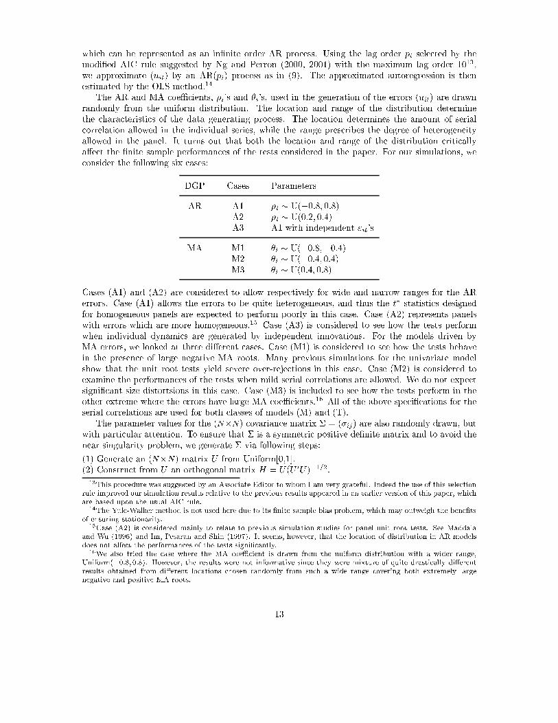
which can be represented as an in�nite order AR process. Using the lag order pi selected by the
modi�ed AIC rule suggested by Ng and Perron (2000, 2001) with the maximum lag order 1013,
we approximate (uit) by an AR(pi) process as in (9). The approximated autoregression is then
estimated by the OLS method.14
The AR and MA coeÆcients, �i's and �i's, used in the generation of the errors (uit) are drawn
randomly from the uniform distribution. The location and range of the distribution determine
the characteristics of the data generating process. The location determines the amount of serial
correlation allowed in the individual series, while the range prescribes the degree of heterogeneity
allowed in the panel. It turns out that both the location and range of the distribution critically
a�ect the �nite sample performances of the tests considered in the paper. For our simulations, we
consider the following six cases:
DGP Cases Parameters
AR A1 �i � U(�0:8; 0:8)A2 �i � U(0:2; 0:4)
A3 A1 with independent "it's
MA M1 �i � U(�0:8;�0:4)M2 �i � U(�0:4; 0:4)M3 �i � U(0:4; 0:8)
Cases (A1) and (A2) are considered to allow respectively for wide and narrow ranges for the AR
errors. Case (A1) allows the errors to be quite heterogeneous, and thus the t� statistics designed
for homogeneous panels are expected to perform poorly in this case. Case (A2) represents panels
with errors which are more homogeneous.15 Case (A3) is considered to see how the tests perform
when individual dynamics are generated by independent innovations. For the models driven by
MA errors, we looked at three di�erent cases. Case (M1) is considered to see how the tests behave
in the presence of large negative MA roots. Many previous simulations for the univariate model
show that the unit root tests yield severe over-rejections in this case. Case (M2) is considered to
examine the performances of the tests when mild serial correlations are allowed. We do not expect
signi�cant size distortsions in this case. Case (M3) is included to see how the tests perform in the
other extreme where the errors have large MA coeÆcients.16 All of the above speci�cations for the
serial correlations are used for both classes of models (M) and (T).
The parameter values for the (N�N) covariance matrix � = (�ij) are also randomly drawn, but
with particular attention. To ensure that � is a symmetric positive de�nite matrix and to avoid the
near singularity problem, we generate � via following steps:
(1) Generate an (N�N) matrix U from Uniform[0,1].
(2) Construct from U an orthogonal matrix H = U(U 0U)�1=2.
13This procedure was suggested by an Associate Editor to whom I am very grateful. Indeed the use of this selection
rule improved our simulation results relative to the previous results appeared in an earlier version of this paper, which
are based upon the usual AIC rule.14The Yule-Walker method is not used here due to its �nite sample bias problem, which may outweigh the bene�ts
of ensuring stationarity.15Case (A2) is considered mainly to relate to previous simulation studies for panel unit root tests. See Maddala
and Wu (1996) and Im, Pesaran and Shin (1997). It seems, however, that the location of distribution in AR models
does not a�ect the performances of the tests signi�cantly.16We also tried the case where the MA coeÆcient is drawn from the uniform distribution with a wider range,
Uniform(�0:8;0:8). However, the results were not informative since they were mixture of quite drastically di�erent
results obtained from di�erent locations chosen randomly from such a wide range covering both extremely large
negative and positive MA roots.
13

(3) Generate a set of N eigen values, �1; : : : ; �N . Let �1=r > 0 and �N=1 and draw �2; : : : ; �N�1from Uniform[r,1].
(4) Form a diagonal matrix � with (�1; : : : ; �N) on the diagonal.
(5) Construct the covariance matrix � as a spectral representation � = H�H 0.
The covariance matrix constructed this way will surely be symmetric and nonsingular with eigen-
values taking values from r to 1. We set the maximum eigenvalue at 1 since the scale does not
matter. The ratio of the minimum eigenvalue to the maximum is therefore determined by the same
parameter r. The covariance matrix becomes singular as r tends to zero, and becomes spherical as
r approaches to 1. For the simulations, we set r at r = 0:1.17
For the test of the unit root hypothesis, we set �i = 0 for all i = 1; : : : ;N , and investigate
the �nite sample sizes in relation to the corresponding nominal test sizes. To examine the rejec-
tion probabilities of the tests under the alternative of stationarity, we generate �i's randomly from
Uniform(�0:8; 0). The model is thus heterogenous under the alternative. The �nite sample perfor-mance of the bootstrap tests are compared with that of the t-bar statistic by Im, Pesaran and Shin
(1997), which is based on the average of the individual t-statistics computed from the sample ADF
regressions (5) with mean and variance modi�cations. More explicitly, the t-bar statistic is de�ned
as
t-bar =
pN(�tN �N
�1P
N
i=1E(ti; pi; �i;1; : : : ; �i;pi))qN�1P
N
i=1 var(ti; pi; �i;1; : : : ; �i;pi)
where ti is the t-statistic for testing �i = 0 for the i-th sample ADF regression (5), and �tN =
N�1P
N
i=1 ti. The values of the expectation and variance, E(ti) and var(ti), for each individ-
ual ti depend on T , the lag order pi and the coeÆcients on the lagged di�erences �i;k 's, and
are computed via simulations from independent normal samples assuming �i;1 = � � � = �i;pi =
0. Table 2 in Im, Pesaran and Shin (1997) tabulates the values of E(ti) and var(ti) for T =
5; 10; 15; 20; 25; 30; 40; 50; 60; 70; 100 and for pi = 1; : : : ; 8. When the AR order pi chosen by the
selection rule is greater than 8, we replace it by 8 for the construction of the t-bar test since the
mean and variance modi�cations are available only for pi's upto 8. However, for the construction of
our bootstrap tests, we use the original order selected by the rule.
The panels with the cross-sectional dimensions N= 5; 10 and the time series dimension T = 100
are considered for the 5% size test. Since we are using random parameter values, we simulate 20
times for each case and report the ranges of the �nite sample performances of the tests. Each
simulation run is carried out with 1,000 simulation iterations, each of which uses bootstrap critical
values computed from 500 bootstrap repetitions. The simulation results for the t-bar statistic and
our bootstrap tests F �
OT, F �
GT, K�
OT, K�
GT, t�
OTand t�
GTfor the models (M) with heterogeneous �xed
e�ects are reported in Tables MS.A1-MP.M3. Tables MS.A1(A2,A3) and MP.A1(A2,A3) report,
respectively, the �nite sample sizes and powers of the tests for case A1(A2,A3) with the AR errors
generated by the DGP de�ned with the parameters given in A1(A2,A3). Tables MS.M1(M2,M3)
and MP.M1(M2,M3) report the �nite sample sizes and powers for case M1(M2,M3) with the MA
errors generated by the DGP M1(M2,M3). Similarly, Tables TS.A1-TP.M3 report the �nite sample
sizes and powers of the tests for the models (T) with individual time trends. For each statistic, we
report the minimum, mean, median and maximum of the rejection probabilities under the null and
under the alternative hypotheses.
In general, the t-bar test su�ers from serious size distortions for both models (M) and (T)
and for all speci�cations of serial correlations considered with cross-sectional dependency. The size
distortions in the models driven by MA errors or with time trends are much more severe than those
17Our bootstrap tests do not seem to depend on the the value of r, but the t-bar statistic does. Though we do
not report the details, we observe from a set of simulations that the t-bar tends to have higher rejection probabilities
when r is close to 0, relative to the case where � is nearly spherical with r = 0:99.
14

in the models driven by AR errors or with �xed e�ects only.18 In particular, it su�ers from huge
upward size distortions for case (M1) with large negative MA roots. As can be seen from Table
MS.M1 for the models (M) with heterogeneous �xed e�ects, the average size of the t-bar tests for
the 5% test is 45% for N=5, and increases to 66% for the larger N=10. For cases (M2) and (M3),
the t-bar continues to over-reject for both N=5,10, though the magnitude of the distortions is much
smaller than in case (M1). See Tables MS.M2 and MS.M3. The t-bar has similar patterns of size
distortions for the models (T) with time trends. However, the degree of distortions are noticeably
magni�ed in this case, especially for the cases generated by MA errors. For instance, as can be
seen from Table TS.M1, the upward distortion in case (M1) is now enormous, and it gets worse as
N increases. For the 5% test, the average size of the t-bar test is 76% for the smaller N=5 and
increases to 94% when the larger N = 10 is used.
On the other hand, the �nite sample sizes of the bootstrap tests are overall quite close to the
nominal test sizes in most of the cases. For the cases with AR errors, all bootstrap tests have very
good size properties for both classes of models (M) and (T), as can be seen from Tables MS.A1(A2)
and TS.A1(A2). Our bootstrap tests also have reasonably good sizes for the cases with MA errors,
except for case (M1). In this case, all bootstrap tests also su�er from upward size distortions;
however, the degree of the distortions in our bootstrap tests is not comparable to that of the t-bar
test. Ours is much less severe than theirs.19 See Tables MS.M1 and TS.M1.
We now turn to �nite sample powers of the tests. In general, it seems that our bootstrap tests
perform satisfactorily in all cases we consider in the paper. It is, however, not easy to directly
compare power performances of our tests with those of the t-bar using the computed rejection
probabilities, since in many cases the t-bar test has signi�cant size distortions. Nonetheless, we can
make straightforward comparisons in some cases. As can be seen from Tables MS.A and MP.A for
cases A1 and A2 for the models with �xed e�ects, the GLS-based bootstrap tests, F �
GTand K�
GT,
perform clearly better than the t-bar test even in the presence of the upward size distortions in the
t-bar test. The bootstrap tests appear to perform quite well relative to the t-bar test also for all
other cases, once we take into account the upward size distortions in the t-bar test. Our bootstrap
tests F � and K� seem to yield better powers than the t-bar test in most of the cases. There are,
however, cases where the t� tests appear less powerful than the t-bar. The performance of the t�
tests varies with the degree of heterogeneity allowed in the model. The �nite sample powers of
all tests are lower for the models (T) with time trends, compared with the models (M) with �xed
e�ects only. We expect that the eÆcient GLS-detrending suggested by Elliot, Rothenberg and Stock
(1996) improves the power properties of our bootstrap tests in both models. However, it is not used
here to give a fair ground to the t-bar test, whose critical values are available only for the usual
OLS-detrending.
We now discuss the relative performances among our bootstrap tests. The GLS-based tests
generally perform better than their OLS counterparts in terms of both sizes and powers. The GLS-
based tests F �
GTand K�
GThave better sizes for all cases except (M1) and are more powerful than
their OLS counterparts F �
OTand K�
OT. This is even more evident for the models (T) with individual
time trends. For the t� tests, however, this is not always the case. The t�GT
seems to have better
sizes than t�OT
in most of the cases, but it is more powerful than t�OT
only for the smaller N . See
the discussion on the t� test below. Overall, the F � and K� tests perform better than the t� test in
terms of both sizes and powers, except for the cases described below.
18In the models with independent AR errors as in case A3, the t-bar performs quite well as expected. However,
even in such cases with cross-sectional independence, the t-bar test starts to over-reject as we introduce time trends
and the upward distortions become more obvious as N increases.19The poor size performances of the tests in case (M1) for both models with �xed e�ects and time trends go in line
with the well known size problems of the univariate unit root tests in models with large negative MA roots. It is also
observed that bootstrap tests reduce, though not completely, the size distortions in such cases. See Chang and Park
(1999).
15

The t-type tests are one-sided tests constructed for homogenous panels. Hence, for our simulation
models with the alternatives drawn heterogeneously for each individual unit, it is well expected that
the t� tests will be less powerful than the F � and K� tests that are designed for heterogeneous
panels. Indeed, when the models allow substantial amount of heterogeneity, as in cases (A1) and
(A3), the t� tests have lower power and exhibit larger variability. However, when the models are
modestly heterogeneous, as in case (A2), the t� tests become much less variable and more powerful,
almost comparable to the F � and K� tests. For the cases with MA errors, the models considered
here are not drastically heterogeneous, and consequently the powers of the t� tests are reasonably
good. We also note that the OLS based t-statistic t�OT
is more powerful than its GLS couterpart t�GT
when the larger N=10 is used, which is not observed for the F � and K� tests.
The K-statistics are proposed as an alternative to the two-sided F -type test to come up with
more powerful tests for the unit roots against the one-way alternative of stationarity. The simulation
results in Tables MP and TP, however, show that the improvement the K-statistics make over
the F -type tests are insigni�cant. The �nite sample distributions of �̂GT and �̂OT , upon which
the modi�cations for the K-statistics are made, are indeed skewed to the left so much that the
modi�cations do not have actual e�ect. For better results, we thus need to correct the biases in
the distributions of �̂GT and �̂OT before applying the modi�cations given in the equation preceding
(11). This can be implemented in practice by carrying out a nested bootstrap, the �rst step of
which involves the bootstrap corrections for the biases in �̂GT and �̂OT . We do not pursue this in
the present paper due to the computation time, but will report in a future work.
5. Conclusion
There has been much recent empirical and theoretical econometric work on models with nonstation-
ary panel data. In particular, much attention has been paid to the development and implementation
of the panel unit root tests which have been used frequently to test for various covergence theories,
such as growth covergence theories and purchasing power parity hypothesis. A variety of tests have
been proposed, including the tests proposed by Levin and Lin (1993) and Im, Pesaran and Shin
(1997) that appear to be most commonly used. All the existing tests, however, assume the inde-
pendence across cross-sectional units, which is quite restrictive for most of economic panel data we
encounter. Cross-sectional dependency seems indeed quite apparent for most of interesting panel
data.
In the paper, we investigate various unit root tests for panel models which explicitly allow for the
cross-correlation across cross-sectional units as well as heterogeneous serial dependence. The limit
theories for the panel unit root tests are derived by passing the number of time series observations
T to in�nity with the number of cross-sectional units N �xed. As expected the limit distributions of
the tests are nonstandard and depend heavily on the nuisance parameters, rendering the standard
inferential procedure invalid. To overcome the inferential diÆculty of the panel unit root tests in
the presence of cross-sectional dependency, we propose to use the bootstrap method. Limit theories
for the bootstrap tests are developed, and in particular their asymptotic validity is established by
proving the consistency of the boostrap tests. The simulations show that the bootstrap panel unit
root tests perform well in �nite samples relative to the t-bar statistic by Im, Pesaran and Shin
(1997).
6. Appendix: Mathematical Proofs
The following lemmas provide asymptotic results for the sample moments appearing in the sample
test statistics FGT , FOT , KGT , KOT , tGT and tOT de�ned in (7), (8), (11), (12) and (14).
16

Lemma A1 Under Assumptions 1 { 3, we have
(a)1
T
NXt=1
yi;t�1"pjjt = �i(1)
1
T
TXt=1
wi;t�1"jt + op(1), for all i; j = 1; : : : ;N
(b)1
T2
TXt=1
yi;t�1yj;t�1 = �i(1)�j(1)1
T2
TXt=1
wi;t�1wj;t�1 + op(1), for all i; j = 1; : : : ;N
(c)1
T
TXt=1
"pt "
p0t =
1
T
TXt=1
"t"0
t + op(1)
Proof of Lemma A1
Part (a) The stated results follow immediately if we apply the results in Lemma 3.1 (a) of Chang
and Park (2001) to each (i; j) pair, for i; j = 1; : : : ;N .
Part (b) The stated result follows directly from Phillips and Solo (1992).
Part (c) Let QT = T�1P
T
t=1 "pt "
p0t � T
�1P
T
t=1 "t"0
t. Then for each (i; j)-element of Q, we have
QT;ij =1
T
TXt=1
("piit � "it)"
pjjt +
1
T
TXt=1
"it("pjjt � "jt) = op(p
�si ) + op(p
�sj )
due to Lemma 3.1 (c) in Chang and Park (2001). Now the stated result is immediate.
Lemma A2 Under Assumptions 1 { 3, we have
(a)
1
T
TXt=1
xpiit x
pi0it
!�1 = Op(1), for all pi and i = 1; : : : ;N
(b)
�����TXt=1
xpiit yj;t�1
����� = Op(Tp1=2i ), for all i; j = 1; : : : ;N
(c)
�����TXt=1
xpiit "
pjjt
����� = Op(T1=2p
1=2i ) + op(Tp
1=2i p�sj ), for all i; j = 1; : : : ;N .
Proof of Lemma A2 The stated result in Part (a) follows directly from the application of the
result in Lemma 3.2 (a) of Chang and Park (2001) for each i = 1; : : : ;N , and those in Parts (b) and
(c) are easily obtained using the results in Lemma 3.2 (b) and (c) of the aforementioned reference for
each (i; j) pair for i; j = 1; : : : ;N , with some obvious modi�cations with respect to the heterogeneous
orders pi's of the AR approximations involved.
Proof of Theorem A.1
Part (a) We begin by examining the stochastic orders of the component sample moments appearing
in AGT and BGT de�ned below (8). Let �(�) denote eigenvalues of a matrix. We have
�min(~��1 IT )X
0
pXp � X 0
p(~��1 IT )Xp
Notice that �min(~��1 IT ) = �min(~�
�1) and �min(~��1) = 1=�max(~�). Then we have
X 0
p(~��1 IT )Xp
T
!�1
� �max(~�)
�X 0
pXp
T
��1= Op(1) (28)
17

since �max(~�) !p �max(�) < 1 and (T�1X 0
pXp)�1 = Op(1) due to Lemma A2 (a). Moreover it
follows from Lemma A2 (b) that
X 0
p(~��1 IT )Y` = Op(T �p
1=2) (29)
where �p = max1�i�N
pi, and from Lemma A2 (c) that
X 0
p(~��1 IT )"p = Op(T
1=2�p1=2) + op(T �p1=2p�s) (30)
where p = min1�i�N
pi. Notice that �p = p = o(T 1=2) as T!1 under Assumption 3.
It follows from (28), (29) and (30) that����Y 0
` (~��1 IT )Xp
�X 0
p(~��1 IT )Xp
��1
X 0
p(~��1 IT )"p
�����
���Y 0
` (~��1 IT )Xp
��� �X 0
p(~��1 IT )Xp
��1 ���X 0
p(~��1 IT )"p
���= op(T �pp
�s) +Op(T1=2�p)
which implies
AGT
T=
Y 0
` (~��1 IT )"p
T+ op(1) = QAGT + op(1) (31)
due to Lemma A1 (a), where
QAGT =
0BBBBBBBB@
NXj=1
~�1j�1(1)1
T
TXt=1
w1;t�1"jt
...NXj=1
~�Nj�N(1)1
T
TXt=1
wN;t�1"jt
1CCCCCCCCA
where ~�ij denotes (i; j)-element of the covariance matrix estimate ~�.
Moreover, we have from (28) and (29) that����Y 0
` (~��1 IT )Xp
�X 0
p(~��1 IT )Xp
��1
X 0
p(~��1 IT )Y`
�����
���Y 0
` (~��1 IT )Xp
��� �X 0
p(~��1 IT )Xp
��1 ���X 0
p(~��1 IT )Y`
��� = Op(T �p)
which, together with Lemma A1 (b) gives
BGT
T2
=Y 0
` (~��1 IT )Y`
T2
+ op(1) = QBGT + op(1) (32)
where
QBGT =
0BBBBBBBB@
~�11�1(1)2 1
T2
TXt=1
w21;t�1 � � � ~�1N�1(1)�N(1)
1
T2
TXt=1
w1;t�1wN;t�1
......
...
~�N1�N(1)�1(1)1
T2
TXt=1
wN;t�1w1;t�1 � � � ~�NN�N(1)2 1
T2
TXt=1
w2N;t�1
1CCCCCCCCA
18

Using the asymptotic results in (31) and (32), we write
FGT =
�AGT
T
�0�BGT
T2
��1�
AGT
T
�= Q0
AGTQ�1BGT
QAGT + op(1)
Then the limit distribution of FGT follows immediately from the invariance principle given in (25).
Part (b) We have from Lemma A2 (b) and (c) that
X 0
pY` = Op(T �p1=2); X 0
p"p = Op(T1=2�p1=2) + op(T �p
1=2p�s) (33)
These together with (28) give��Y 0
`Xp(X0
pXp)�1X 0
p"p�� � jY 0
`Xpj (X 0
pXp)�1 ��X 0
p"p�� = op(T �pp
�s) +Op(T1=2�p)
which in turn givesAOT
T=
Y 0
` "p
T+ op(1) = QAOT + op(1) (34)
due to Lemma A1 (a), where
QAOT =
0BBBBBBBB@
�1(1)1
T
TXt=1
w1;t�1"1t
...
�N(1)1
T
TXt=1
wN;t�1"Nt
1CCCCCCCCA
We have from (28) that
X 0
p(~� IT )Xp � �max(~�)(X
0
pXp) = Op(T ) (35)
Also it follows from Lemma A2 (b) that X 0
p(~� IT )Y` = Op(T �p
1=2).
Then we have���Y 0
`Xp(X0
pXp)�1X 0
p(~� IT )Y`
��� = Op(T �p) and���Y 0
`Xp(X0
pXp)�1X 0
p(~� IT )Xp(X
0
pXp)�1X 0
pY`
��� = Op(T �p)
which in turn give
MFOT
T2
=Y 0
` (~� IT )Y`
T2
+ op(1) = QMFOT+ op(1) (36)
due to Lemma A1 (b), where
QMFOT=
0BBBBBBBB@
~�11�1(1)2 1
T2
TXt=1
w21;t�1 � � � ~�1N�1(1)�N(1)
1
T2
TXt=1
w1;t�1wN;t�1
......
...
~�N1�N(1)�1(1)1
T2
TXt=1
wN;t�1w1;t�1 � � � ~�NN�N(1)2 1
T2
TXt=1
w2N;t�1
1CCCCCCCCA
We now have from the results in (34) and (36) that
FOT =
�AOT
T
�0�MFOT
T2
��1�
AOT
T
�= Q0
AOTQ�1MFOT
QAOT + op(1)
19

from which the stated result follows immediately.
Proof of Corollary A.1
Part (a) It follows from (31) and (32) that
T �̂GT =
�BGT
T2
��1�
AGT
T
�= Q�1
BGTQAGT + op(1)
which implies
1
T
�AGT :� 1f�̂GT � 0g
�=
�AGT
T:� 1��̂GT
T� 0
��=�QAGT :� 1
�Q�1BGT
QAGT � 0�
+ op(1)
Due to the above result and (32), we may write the KGT statistic given in (11) as
KGT =
�1
T
�AGT :� 1f�̂GT � 0g
��0�BGT
T2
��1�
1
T
�AGT :� 1f�̂GT � 0g
��
=�QAGT :� 1
�Q�1BGT
QAGT � 0�
0
Q�1BGT
�QAGT :� 1
�Q�1BGT
QAGT � 0�
+ op(1)
Now the stated result follows immediately from (25).
Part (b) From (28) and (33), we have��Y 0
`Xp(X0
pXp)�1X 0
pY`�� = Op(T �p); which together with
Lemma A1 (b) givesBOT
T2
=Y 0
`Y`
T2
+ op(1) = QBOT + op(1)
where
QBOT =
0BBBBBBBB@
�1(1)2 1
T2
TXt=1
w21;t�1 � � � �1(1)�N(1)
1
T2
TXt=1
w1;t�1wN;t�1
......
...
�N(1)�1(1)1
T2
TXt=1
wN;t�1w1;t�1 � � � �N(1)2 1
T2
TXt=1
w2N;t�1
1CCCCCCCCA
(37)
It follows from (34) and the above result that
T �̂OT =
�BOT
T2
��1�
AOT
T
�= Q�1
BOTQAOT + op(1)
and1
T
�AOT :� 1f�̂OT � 0g
�=�QAOT :� 1
�Q�1BOT
QAOT � 0�
+ op(1)
From this and the result in (36), we may express the statistic KOT given in (12) as
KOT =
�1
T
�AOT :� 1f�̂OT � 0g
��0�MFOT
T2
��1�
1
T
�AOT :� 1f�̂OT � 0g
��
=�QAOT :� 1
�Q�1BOT
QAOT � 0�
0
Q�1MFOT
�QAOT :� 1
�Q�1BOT
QAOT � 0�
+ op(1)
which is required for the stated result.
20

Proof of Theorem A.2 The limit theories for the GLS and OLS based t-statistics tGT and tOTde�ned in (14) can be derived in the similar manner as we did for the F -type tests FGT and FOT in
the proof of Theorem A.1. We just have to take into account that the lagged level variables come
in as an (NT � 1)-vector y` instead of the (NT � N)-matrix Y`.
Part (a) We begin by examining the sample moments appearing in aGT and bGT , de�ned below
(14). Since X 0
p(~��1 IT )y` = Op(T �p
1=2) due to Lemma A2 (b), it follows from (28) and (30) that
����y0`(~��1 IT )Xp
�X 0
p(~��1 IT )Xp
��1
X 0
p(~��1 IT )"p
���� = op(T �pp�s) +Op(T
1=2�p)
and ����y0`(~��1 IT )Xp
�X 0
p(~��1 IT )Xp
��1
X 0
p(~��1 IT )y`
���� = Op(T �p)
Then from the above results and Lemma A1 (a) and (b), it follows that
aGT
T=
y0`(~��1 IT )"p
T+ op(1) =
NXi=1
NXj=1
~�ij1
T
TXt=1
yi;t�1"pjjt + op(1) = QaGT + op(1)
bGT
T2
=y0`(
~��1 IT )y`
T2
+ op(1) =
NXi=1
NXj=1
~�ij1
T2
TXt=1
yi;t�1yj;t�1 + op(1) = QbGT + op(1)
where
QaGT =
NXi=1
NXj=1
~�ij�i(1)1
T
TXt=1
wi;t�1"jt
QbGT =
NXi=1
NXj=1
~�ij�i(1)�j(1)1
T2
TXt=1
wi;t�1wj;t�1
We may now write tGT de�ned in (14) as follows
tGT =aGT
T
�bGT
T2
��1=2
= QaGTQ�1=2
bGT+ op(1)
and the limit theory for tGT is directly obtained from applying the invariance principle in (25) to
QaGT and QbGT .
Part (b) Again, we �rst analyze the components aOT andMtOT , de�ned below (14), that constitute
the OLS based t-statistic tOT given in (14). Since
X 0
py` = Op(T �p1=2) and X 0
p(~� IT )y` = Op(T �p
1=2)
by Lemma A2 (b), we have from (35) that��Y 0
`Xp(X0
pXp)�1X 0
p"p�� = op(T �pp
�s) +Op(T1=2�p)���Y 0
`Xp(X0
pXp)�1X 0
p(~� IT )Y`
��� = Op(T �p)���Y 0
`Xp(X0
pXp)�1X 0
p(~� IT )Xp(X
0
pXp)�1X 0
pY`
��� = Op(T �p)
21

We now deduce from Lemma A1 (a) and (b) that
aOT
T=
y0`"p
T+ op(1) =
NXi=1
1
T
TXt=1
yi;t�1"piit + op(1) = QaOT + op(1)
MtOT
T2
=y0`(
~� IT )y`
T2
+ op(1) =
NXi=1
NXj=1
~�ij1
T2
TXt=1
yi;t�1yj;t�1 + op(1) = QMtOT+ op(1)
where
QaOT =
NXi=1
�i(1)1
T
TXt=1
wi;t�1"it
QMtOT=
NXi=1
NXj=1
~�ij�i(1)�j(1)1
T2
TXt=1
wi;t�1wj;t�1
Then we have
tOT =aOT
T
�MtOT
T2
��1=2
= QaOTQ�1=2
MtOT+ op(1)
from which the stated result follows immediately.
Proofs for the Bootstrap Asymptotics
In the following lemma, we use an operator norm for matrices: if C = (cij) is a matrix, then we
let kCk = maxx jCxj=jxj.Lemma B2 Let x
�piit = (4y�i;t�1; : : : ;4y�i;t�pi)
0. Then we have
(a) E�
1
T
TXt=1
x�piit x
�pi0it
!�1 = Op(1), for all i = 1; : : : ;N .
(b) E�
�����TXt=1
x�piit y�j;t�1
����� = O(Tp1=2i ) a:s:, for all i; j = 1; : : : ;N .
(c) E�
�����TXt=1
x�piit "�jt
����� = O(T 1=2p1=2i ) a:s:, for all i; j = 1; : : : ;N .
under Assumptions 1 { 3.
Proofs of Lemmas B1 and B2 The stated results follow directly from Lemmas 3.2 and 3.3 of
Chang and Park (1999), and thus omitted.
Proof of Theorem B.1 The proof here follows closely the lines of the proof of Theorem A.1,
using the bootstrap asymptotics established in Lemmas 1 and 2.
Part (a) From Lemma 2 (a), we have X�0
p (~��1 IT )X
�
p
T
!�1
� �max(~�)
�X�0
p X�
p
T
��1= O�
p(1) (38)
which along with the results in Lemma B1 (b) and Lemma B2 (b) and (c) gives
A�GT
T= Y �0
` (~��1 IT )"� + o�p(1) = QA�
GT+ o�p(1) (39)
22

in P under Assumptions 1 { 3, where QA�
GTis de�ned similarly as QAGT in (31) with ~�i(1); w
�
it and
"�it in the places of �i(1); wit and "it. Similarly, we have from (38), Lemma B1 (b) and Lemma 2
(b) thatB�
GT
T2
= Y �0
` (~��1 IT )Y�
` + o�p(1) = QB�
GT+ o�p(1) (40)
in P under Assumptions 1 { 3, analogously as before, where QB�
GTis de�ned similarly as QBGT
given below (32) with ~�i(1) and w�it in the places of �i(1) and wit, respectively.
We now write the bootstrapped statistic F �
GTas
F �
GT=
�A�GT
T
�0�B�
GT
T2
��1�
A�GT
T
�= Q0
A�
GTQ�1B�
GT
QA�
GT+ o�p(1)
due to (39) and (40). It is shown in Park (1999) that
~�i(1)!a:s: �i(1) (41)
and, using the multivariate bootstrap invariance principle developed in Chang, Park and Song (2000),
we have1
T
TXt=1
w�t�1"�0
t !d�
Z 1
0
BdB0 a:s:;1
T2
TXt=1
w�t�1w�0
t�1 !d�
Z 1
0
BB0 a:s: (42)
under Assumptions 1 { 3. Now, the limiting distribution of the F �
GTfollows immediately.
Part (b) It follows from Lemma 2 (b) and (c) that
X�0
p Y�
` = O�
p(T �p1=2); X�0
p "� = O�
p(T1=2�p1=2) (43)
which together with (38) and Lemma B1 (a) implies that
A�OT
T=
Y �0
` "�
T+ o�p(1) = QA�
OT+ o�p(1) (44)
where QA�
OTis de�ned similarly as QAOT in (34) with the bootstrap samples and ~�(1).
Next, we deduce from (38) and Lemma 2 (b) that
X�0
p (~� IT )X
�
p = O�
p(T�1); X�0
p (~� IT )Y
�
` = O�
p(T �p1=2) (45)
and this together with (43) gives
M�
FOT
T2
=Y �0
` (~� IT )Y�
`
T2
+ o�p(1) = QM�
FOT+ o�p(1) (46)
due to Lemma B1 (b), where QM�
FOTis the bootstrap counterpart of QMFOT
given in (36).
Finally, we have from the results in (45) and (46)
F �
OT=
�A�OT
T
�0�M�
FOT
T2
��1�
A�OT
T
�= Q0
A�
OTQ�1M�
FOT
QA�
OT+ o�p(1)
and the stated result now follows immediately from (41) and (42).
Proof of Corollary B.1 The proof is analogous to the proof of Corollary A.1.
Part (a) We have from the bootstrap asymptotic results established in (39) and (40) that
23

T �̂�GT
=
�B�
GT
T2
��1�
A�GT
T
�= Q�1
B�
GT
QA�
GT+ o�p(1)
Then we may write the K�
GTstatistic given in (22) as
K�
GT=
�1
T
�A�GT
:� 1f�̂�GT� 0g
��0�B�
GT
T2
��1�
1
T
�A�GT
:� 1f�̂�GT� 0g
��
=�QA�
GT:� 1nQ�1B�
GT
QA�
GT� 0o�
0
Q�1B�
GT
�QA�
GT:� 1nQ�1B�
GT
QA�
GT� 0o�
+ o�p(1)
Now the stated result follows immediately from (41) and (42).
Part (b) Using the bootstrap asymptotic results in (38), (43) and Lemma B1 (b), we derive
B�
OT
T2
=Y �0
` Y �
`
T2
+ op(1) = QB�
OT+ op(1)
where QB�
OTis the bootstrap counterpart of QBOT de�ned in (37). Similarly as in the proof of
Corollary A.1 (b), we may write the test K�
OTgiven in (22) as
K�
OT=
�1
T
�A�OT
:� 1f�̂�OT� 0g
��0�M�
FOT
T2
��1�
1
T
�A�OT
:� 1f�̂�OT� 0g
��
=�QA�
OT:� 1nQ�1B�
OT
QA�
OT� 0o�
0
Q�1M�
FOT
�QA�
OT:� 1nQ�1B�
OT
QA�
OT� 0o�
+ o�p(1)
using the result in (46). The stated result now follows immediately from (41) and (42).
Proof of Theorem B.2 The limit distributions of the bootstrap GLS and OLS based t-statistics,
t�GT
and t�OT, de�ned in (24) are derived analogously as we did for the sample t-statistics tGT and
tOT in the proof of Theorem A.2, using the bootstrap asymptotics established in Lemmas 1 and 2.
Part (a) It follows from Lemmas 1 and 2, and the result in (38) that
a�GT
T=
y�0` (~��1 IT )"
�
T+ o�p(1) = Qa�
GT+ o�p(1)
b�GT
T2
=y�0` (
~��1 IT )y�
`
T2
+ o�p(1) = Qb�GT
+ o�p(1)
where Qa�GT
and Qb�GT
are the bootstrap counterparts of QaGT and QbGT de�ned in the proof of
Theorem A.2 (a). We may now write t�GT
as
t�GT
=a�GT
T
�b�GT
T2
��1=2
= Qa�GTQ�1=2
b�GT
+ o�p(1)
and the limit theory for t�GT
is directly obtained from (41) and (42).
Part (b) We have
X�0
p y�
` = O�
p(T �p1=2); X�0
p (~� IT )y
�
` = O�
p(T �p1=2)
by Lemma A2 (b). Then we may deduce from Lemma B1 and (45) that
a�OT
T=
y�0` "�
T+ o�p(1) = Qa�
OT+ o�p(1)
M�
tOT
T2
=y�0` (
~� IT )y�
`
T2
+ o�p(1) = QM�
tOT+ o�p(1)
24

where Qa�OT
and QM�
tOTare the bootstrap counterparts to QaOT and QMtOT
given in the proof of
Theorem A.2 (b). Then we have
t�OT
=a�OT
T
�M�
tOT
T2
��1=2
= Qa�OTQ�1=2
M�
tOT
+ o�p(1)
The stated result now follows immediately from (41) and (42).
7. References
Andrews, D.W.K. (1999). \Estimation when a parameter is on a boundary," Econometrica, 67,
1341-1383.
Baltagi, B.H. (1995). Econometric Analysis of Panel Data. Wiley: Chichester.
Basawa, I.V., A.K. Mallik, W.P. McCormick, J.H. Reeves and R.L. Taylor (1991). \Bootstrapping
unstable �rst-order autoregressive processes," Annals of Statistics, 19, 1098-1101.
Banerjee, A. (1999). \Panel data unit roots and cointegration: An Overview," Oxford Bulletin of
Economics & Statistics, 61, 607-629.
Brillinger, D.R. (1975). Time Series: Data Analysis and Theory. Holt, Rinehart and Winston:
New York.
Brockwell, P.J. and R.A. Davis (1991). Time Series: Theory and Methods. Springer-Verlag: New
York.
Chang, Y. and J.Y. Park (1999). \A sieve bootstrap for the test of a unit root," forthcoming in
Journal of Time Series Analysis.
Chang, Y. and J.Y. Park (2001). \On the asymptotics of ADF tests for unit roots," mimeographed,
Department of Economics, Rice University.
Chang, Y., J.Y. Park and K.M. Song (2000). \Bootstrapping cointegrating regressions," mimeographed,
Department of Economics, Rice University.
Chang, Y., R. Sickles and W. Song (2000). \Bootstrapping unit root tests with covariates,"
mimeographed, Department of Economics, Rice University.
Elliot, G., T.J. Rothenberg and J.H. Stock (1992). \EÆcient tests for an autoregressive unit root,"
Econometrica, 64, 813-836.
Fisher, R.A. (1933). Statistical Methods for Research Workers. Oliver and Boyd, Edinburgh, 4th
Edition.
Hsiao, C. (1986). Analysis of Panel Data. Cambridge University Press: Cambridge.
Im, K.S., M.H. Pesaran and Y. Shin (1997). \Testing for unit roots in heterogeneous panels,"
mimeographed.
Pesaran, M.H. and R. Smith (1995). \Estimating long-run relationship from dynamic heterogeneous
panels," Journal of Econometrics, 68, 79-113.
Levin, A. and C.F. Lin (1992). \Unit root tests in panel data: Asymptotic and �nite sample
properties," University of California, San Diego, mimeographed.
25

Levin, A. and C.F. Lin (1993). \Unit root tests in panel data: New results," University of California,
San Diego, mimeographed.
McCoskey, S. and C. Kao (1998). \A residual based test for the null of cointegration in panel
data," Econometric Reviews, 17, 57-84.
Maddala, G.S. and S. Wu (1996). \A comparative study of unit root tests with panel data and a new
simple test: Evidence from siulations and bootstrap". Ohio State University, mimeographed.
Matyas, L. and P. Sevestre (eds.) (1996). The Econometrics of Panel Data, Kluwer Academic
Publishers: Boston.
Ng, S. and P. Perron (2000). \Lag length selection and the construction of unit root tests with
good size and power," forthcoming in Econometrica.
Ng, S. and P. Perron (2001). \A note on the selection of time series models," mimeographed,
Boston College.
Park, J.Y. (1999). \An invariance principle for sieve bootstrap in time series". Forthcoming in
Econometric Theory.
Pedroni, P. (1996). \Fully modi�ed OLS for heterogeneous cointegrated panels and the case of
purchasing power parity," Indiana University, mimeographed.
Pedroni, P. (1997). \Panel cointegration: Asymptotic and �nite sample properties of pooled time
series tests with an application to the PPP hypothesis, New results," University of Indiana,
mimeographed.
Phillips, P.C.B. and H.R. Moon (1999). \Linear regression limit theory for nonstationary panel
data," Econometrica, 67, 1057-1111.
Phillips, P.C.B. and V. Solo (1992). \Asymptotics for linear processes," Annals of Statistics, 20,
971-1001.
Quah, D. (1994). \Exploiting cross-section variations for unit root inference in dynamic data,"
Economics Letters, 7, 175-189.
Said, S.E. and D.A. Dickey (1984). \Testing for unit roots in autoregressive-moving average models
of unknown order," Biometrika, 71, 599-608.
Shao, Q.-M. (1995). \Strong approximation theorems for independent random variables and their
applications," Journal of Multivariate Analysis, 52, 107-130.
26

Table MS.A: Finite Sample Sizes for AR Errors, Demeaned Case
(A1) �i �U(�0:8; 0:8) (A2) �i �U(0:2; 0:4) (A3) �i �U(�0:8; 0:8), ID
N T tests min mean med max min mean med max min mean med max
5 100 t-bar 0.052 0.069 0.070 0.082 0.055 0.070 0.070 0.085 0.040 0.053 0.052 0.074
F �GT
0.042 0.054 0.054 0.072 0.042 0.054 0.052 0.070 0.036 0.051 0.051 0.065
F �OT 0.041 0.054 0.055 0.067 0.043 0.054 0.054 0.069 0.040 0.055 0.055 0.064
K�GT 0.041 0.054 0.055 0.074 0.041 0.053 0.052 0.071 0.036 0.051 0.051 0.065
K�OT
0.040 0.055 0.055 0.067 0.043 0.054 0.055 0.068 0.040 0.055 0.055 0.065
t�GT 0.037 0.050 0.050 0.061 0.039 0.049 0.049 0.064 0.037 0.051 0.053 0.062
t�OT 0.036 0.051 0.050 0.066 0.040 0.053 0.054 0.068 0.039 0.054 0.055 0.069
10 100 t-bar 0.061 0.073 0.074 0.086 0.054 0.072 0.072 0.084 0.046 0.056 0.056 0.070
F �GT 0.044 0.054 0.054 0.064 0.037 0.054 0.053 0.068 0.045 0.053 0.051 0.064
F�OT 0.042 0.058 0.059 0.070 0.047 0.057 0.057 0.066 0.050 0.061 0.061 0.074
K�GT 0.044 0.055 0.055 0.065 0.036 0.054 0.054 0.069 0.044 0.054 0.052 0.065
K�OT 0.045 0.058 0.058 0.070 0.045 0.057 0.057 0.068 0.050 0.061 0.061 0.074
t�GT
0.037 0.053 0.053 0.071 0.048 0.057 0.058 0.069 0.039 0.058 0.058 0.075
t�OT
0.039 0.056 0.057 0.071 0.043 0.059 0.060 0.074 0.044 0.064 0.067 0.078
Table MP.A: Finite Sample Powers for AR Errors, Demeaned Case
(A1) �i �U(�0:8; 0:8) (A2) �i �U(0:2; 0:4) (A3) �i �U(�0:8; 0:8), ID
N T tests min mean med max min mean med max min mean med max
5 100 t-bar 0.549 0.856 0.885 0.992 0.522 0.842 0.901 0.989 0.568 0.873 0.913 0.997
F �GT
0.479 0.863 0.929 0.998 0.447 0.844 0.907 0.992 0.457 0.833 0.888 0.993
F �OT 0.354 0.726 0.723 0.952 0.326 0.695 0.701 0.928 0.462 0.842 0.900 0.997
K�GT 0.480 0.863 0.929 0.998 0.448 0.845 0.909 0.993 0.462 0.834 0.889 0.993
K�OT 0.357 0.728 0.724 0.952 0.326 0.697 0.702 0.930 0.464 0.843 0.901 0.997
t�GT 0.066 0.558 0.562 0.994 0.346 0.727 0.747 0.996 0.103 0.633 0.663 0.992
t�OT
0.093 0.584 0.580 0.911 0.231 0.655 0.635 0.961 0.144 0.664 0.711 0.991
10 100 t-bar 0.949 0.987 0.994 1.000 0.939 0.983 0.993 1.000 0.963 0.992 0.997 1.000
F �GT
0.917 0.989 0.999 1.000 0.900 0.985 0.997 1.000 0.897 0.976 0.990 1.000
F �OT
0.801 0.945 0.963 0.998 0.770 0.930 0.958 0.992 0.918 0.982 0.993 1.000
K�GT 0.917 0.989 0.999 1.000 0.901 0.986 0.997 1.000 0.901 0.977 0.991 1.000
K�OT
0.806 0.946 0.964 0.998 0.775 0.932 0.960 0.992 0.921 0.982 0.993 1.000
t�GT
0.121 0.584 0.669 0.964 0.495 0.836 0.856 0.993 0.250 0.732 0.813 0.993
t�OT
0.347 0.770 0.837 0.985 0.722 0.910 0.907 0.992 0.359 0.796 0.873 0.995
27

Table MS.M: Finite Sample Sizes for MA Errors, Demeaned Case
(M1) �i �U(�0:8;�0:4) (M2) �i �U(�0:4; 0:4) (M3) �i �U(0:4; 0:8)
N T tests min mean med max min mean med max min mean med max
5 100 t-bar 0.290 0.450 0.434 0.638 0.087 0.107 0.103 0.152 0.091 0.100 0.100 0.115
F �GT 0.117 0.179 0.174 0.275 0.046 0.057 0.057 0.071 0.046 0.056 0.053 0.067
F �OT 0.090 0.142 0.139 0.219 0.047 0.064 0.065 0.084 0.045 0.057 0.057 0.068
K�GT
0.116 0.180 0.175 0.276 0.046 0.057 0.057 0.069 0.045 0.056 0.053 0.068
K�OT 0.090 0.142 0.139 0.217 0.048 0.064 0.065 0.084 0.045 0.057 0.057 0.069
t�GT 0.125 0.172 0.161 0.258 0.052 0.060 0.059 0.074 0.046 0.058 0.058 0.068
t�OT 0.105 0.139 0.137 0.200 0.051 0.063 0.061 0.074 0.049 0.059 0.059 0.073
10 100 t-bar 0.505 0.663 0.651 0.812 0.102 0.130 0.134 0.161 0.099 0.121 0.121 0.142
F �GT 0.176 0.268 0.268 0.343 0.045 0.059 0.059 0.071 0.041 0.054 0.053 0.067
F�OT 0.173 0.228 0.230 0.291 0.061 0.074 0.075 0.089 0.056 0.066 0.067 0.077
K�GT 0.179 0.269 0.269 0.345 0.044 0.059 0.058 0.072 0.043 0.053 0.052 0.068
K�OT
0.178 0.230 0.232 0.295 0.062 0.074 0.074 0.089 0.055 0.066 0.067 0.078
t�GT
0.190 0.251 0.245 0.322 0.049 0.067 0.070 0.080 0.041 0.069 0.068 0.089
t�OT
0.153 0.203 0.200 0.246 0.044 0.070 0.072 0.082 0.047 0.068 0.069 0.087
Table MP.M: Finite Sample Powers for MA Errors, Demeaned Case
(M1) �i �U(�0:8;�0:4) (M2) �i �U(�0:4; 0:4) (M3) �i �U(0:4; 0:8)
N T tests min mean med max min mean med max min mean med max
5 100 t-bar 0.960 0.994 0.998 1.000 0.629 0.896 0.936 0.995 0.581 0.824 0.845 0.957
F �GT
0.885 0.976 0.986 1.000 0.573 0.880 0.921 0.990 0.467 0.789 0.819 0.951
F �OT 0.764 0.945 0.968 0.999 0.443 0.777 0.792 0.961 0.363 0.671 0.661 0.891
K�GT 0.885 0.976 0.986 1.000 0.574 0.881 0.923 0.990 0.467 0.791 0.820 0.951
K�OT 0.766 0.946 0.968 0.999 0.444 0.779 0.796 0.961 0.367 0.673 0.661 0.894
t�GT 0.653 0.940 0.984 1.000 0.315 0.761 0.821 0.999 0.418 0.719 0.721 0.969
t�OT 0.461 0.900 0.949 1.000 0.241 0.714 0.734 0.961 0.280 0.645 0.592 0.937
10 100 t-bar 1.000 1.000 1.000 1.000 0.964 0.993 0.998 1.000 0.851 0.961 0.972 0.998
F �GT 0.997 1.000 1.000 1.000 0.931 0.989 0.996 1.000 0.833 0.948 0.969 0.995
F �OT
0.991 0.999 1.000 1.000 0.844 0.966 0.984 0.998 0.727 0.890 0.913 0.981
K�GT 0.997 1.000 1.000 1.000 0.932 0.989 0.996 1.000 0.835 0.949 0.970 0.995
K�OT 0.991 0.999 1.000 1.000 0.847 0.967 0.984 0.998 0.734 0.893 0.917 0.982
t�GT 0.878 0.984 0.998 1.000 0.474 0.860 0.951 0.994 0.560 0.828 0.856 0.994
t�OT
0.942 0.991 0.999 1.000 0.735 0.929 0.946 0.996 0.571 0.871 0.875 0.989
28

Table TS.A: Finite Sample Sizes for AR Errors, Detrended Case
(A1) �i �U(�0:8; 0:8) (A2) �i �U(0:2; 0:4) (A3) �i �U(�0:8; 0:8), ID
N T tests min mean med max min mean med max min mean med max
5 100 t-bar 0.076 0.086 0.084 0.102 0.068 0.087 0.085 0.108 0.054 0.066 0.068 0.076
F �GT 0.034 0.049 0.049 0.060 0.037 0.050 0.050 0.060 0.039 0.050 0.050 0.060
F �OT 0.041 0.053 0.052 0.075 0.043 0.053 0.052 0.070 0.042 0.054 0.056 0.063
K�GT
0.034 0.049 0.049 0.060 0.037 0.050 0.050 0.060 0.039 0.050 0.050 0.060
K�OT 0.041 0.053 0.052 0.075 0.043 0.053 0.052 0.070 0.042 0.055 0.056 0.063
t�GT 0.033 0.045 0.045 0.059 0.039 0.052 0.051 0.062 0.039 0.047 0.048 0.058
t�OT 0.034 0.048 0.049 0.059 0.038 0.052 0.052 0.067 0.032 0.050 0.050 0.064
10 100 t-bar 0.080 0.095 0.092 0.118 0.074 0.097 0.099 0.115 0.061 0.075 0.076 0.095
F �GT 0.039 0.053 0.053 0.061 0.038 0.053 0.055 0.065 0.036 0.052 0.052 0.063
F�OT 0.047 0.064 0.065 0.076 0.052 0.065 0.065 0.080 0.063 0.073 0.073 0.084
K�GT 0.039 0.053 0.053 0.061 0.038 0.053 0.055 0.065 0.036 0.052 0.052 0.063
K�OT
0.047 0.064 0.066 0.076 0.052 0.064 0.065 0.080 0.063 0.073 0.073 0.084
t�GT
0.037 0.050 0.049 0.068 0.046 0.058 0.058 0.083 0.043 0.052 0.051 0.071
t�OT
0.038 0.058 0.057 0.078 0.058 0.069 0.069 0.084 0.046 0.063 0.064 0.079
Table TP.A: Finite Sample Powers for AR Errors, Detrended Case
(A1) �i �U(�0:8; 0:8) (A2) �i �U(0:2; 0:4) (A3) �i �U(�0:8; 0:8), ID
N T tests min mean med max min mean med max min mean med max
5 100 t-bar 0.335 0.651 0.655 0.911 0.324 0.633 0.670 0.875 0.313 0.663 0.672 0.928
F �GT
0.240 0.626 0.677 0.899 0.225 0.599 0.633 0.857 0.224 0.580 0.609 0.866
F �OT 0.176 0.485 0.471 0.777 0.169 0.453 0.445 0.723 0.247 0.612 0.637 0.894
K�GT 0.240 0.626 0.677 0.899 0.225 0.599 0.633 0.857 0.224 0.580 0.609 0.866
K�OT 0.176 0.485 0.471 0.777 0.169 0.453 0.445 0.723 0.247 0.612 0.638 0.894
t�GT 0.038 0.331 0.282 0.874 0.199 0.487 0.459 0.852 0.059 0.391 0.342 0.867
t�OT 0.052 0.342 0.338 0.672 0.146 0.419 0.410 0.759 0.080 0.430 0.392 0.879
10 100 t-bar 0.707 0.884 0.899 0.980 0.682 0.864 0.883 0.968 0.720 0.897 0.918 0.993
F �GT 0.636 0.877 0.895 0.984 0.586 0.847 0.863 0.963 0.580 0.815 0.825 0.965
F �OT
0.534 0.778 0.804 0.958 0.499 0.739 0.772 0.895 0.636 0.865 0.887 0.988
K�GT 0.636 0.877 0.895 0.984 0.586 0.847 0.863 0.963 0.580 0.815 0.825 0.965
K�OT 0.534 0.778 0.804 0.957 0.499 0.739 0.772 0.895 0.636 0.865 0.887 0.988
t�GT 0.062 0.280 0.293 0.710 0.331 0.604 0.626 0.872 0.165 0.422 0.425 0.755
t�OT
0.248 0.501 0.508 0.767 0.495 0.714 0.699 0.905 0.248 0.537 0.548 0.841
29

Table TS.M: Finite Sample Sizes for MA Errors, Detrended Case
(M1) �i �U(�0:8;�0:4) (M2) �i �U(�0:4; 0:4) (M3) �i �U(0:4; 0:8)
N T tests min mean med max min mean med max min mean med max
5 100 t-bar 0.599 0.755 0.732 0.906 0.135 0.183 0.182 0.235 0.164 0.179 0.178 0.208
F �GT 0.120 0.159 0.159 0.192 0.051 0.071 0.072 0.089 0.046 0.063 0.064 0.078
F �OT 0.085 0.112 0.110 0.143 0.058 0.080 0.082 0.099 0.047 0.069 0.067 0.084
K�GT
0.120 0.159 0.159 0.192 0.051 0.071 0.072 0.089 0.046 0.063 0.064 0.078
K�OT 0.085 0.112 0.110 0.143 0.058 0.080 0.082 0.099 0.047 0.069 0.067 0.084
t�GT 0.176 0.225 0.218 0.315 0.061 0.071 0.071 0.085 0.057 0.070 0.070 0.087
t�OT 0.124 0.162 0.161 0.219 0.054 0.074 0.070 0.097 0.052 0.067 0.068 0.083
10 100 t-bar 0.857 0.937 0.948 0.988 0.228 0.262 0.255 0.325 0.228 0.246 0.249 0.265
F �GT 0.171 0.219 0.227 0.281 0.060 0.072 0.071 0.092 0.051 0.063 0.061 0.076
F�OT 0.152 0.193 0.195 0.229 0.088 0.104 0.102 0.119 0.079 0.088 0.087 0.102
K�GT 0.171 0.219 0.227 0.281 0.060 0.072 0.071 0.092 0.051 0.063 0.061 0.076
K�OT
0.152 0.194 0.196 0.229 0.088 0.104 0.102 0.119 0.079 0.088 0.087 0.102
t�GT
0.293 0.354 0.356 0.416 0.077 0.091 0.090 0.108 0.080 0.095 0.097 0.110
t�OT
0.263 0.299 0.290 0.344 0.082 0.109 0.108 0.136 0.084 0.097 0.098 0.109
Table TP.M: Finite Sample Powers for MA Errors, Detrended Case
(M1) �i �U(�0:8;�0:4) (M2) �i �U(�0:4; 0:4) (M3) �i �U(0:4; 0:8)
N T tests min mean med max min mean med max min mean med max
5 100 t-bar 0.954 0.991 0.997 1.000 0.489 0.788 0.825 0.965 0.466 0.694 0.708 0.865
F �GT
0.568 0.834 0.867 0.963 0.326 0.680 0.710 0.905 0.268 0.544 0.554 0.780
F �OT 0.412 0.757 0.760 0.932 0.296 0.581 0.576 0.832 0.235 0.459 0.443 0.681
K�GT 0.568 0.834 0.867 0.963 0.326 0.680 0.710 0.905 0.268 0.544 0.554 0.780
K�OT 0.412 0.757 0.760 0.932 0.296 0.581 0.576 0.832 0.235 0.459 0.443 0.682
t�GT 0.468 0.842 0.910 0.995 0.214 0.576 0.592 0.954 0.275 0.506 0.475 0.831
t�OT 0.362 0.770 0.814 0.974 0.195 0.524 0.542 0.828 0.203 0.436 0.400 0.727
10 100 t-bar 0.999 1.000 1.000 1.000 0.840 0.956 0.972 0.996 0.796 0.911 0.927 0.972
F �GT 0.891 0.963 0.976 0.999 0.674 0.902 0.940 0.982 0.527 0.780 0.821 0.911
F �OT
0.874 0.969 0.982 0.998 0.640 0.869 0.903 0.978 0.527 0.749 0.768 0.887
K�GT 0.891 0.963 0.976 0.999 0.674 0.902 0.940 0.982 0.527 0.780 0.821 0.911
K�OT 0.874 0.969 0.982 0.998 0.640 0.869 0.903 0.978 0.528 0.749 0.768 0.887
t�GT 0.783 0.942 0.984 0.996 0.370 0.691 0.778 0.920 0.464 0.679 0.663 0.916
t�OT
0.914 0.967 0.983 0.999 0.612 0.806 0.827 0.964 0.600 0.750 0.748 0.907
30


