
Can the Limitations of Panel Datasets be Overcome by Using Pseudo-Panels to Estimate Income Mobility?
Gary Fields Cornell University and IZA
Mariana Viollaz
CEDLAS-CONICET Universidad Nacional de La Plata
April, 2013
Abstract This paper analyzes whether pseudo panels are suitable substitutes for true panels for estimating income mobility. We obtain evidence using Chilean panel data for the period 1996-2006 and constructing pseudo panels treating each round of the panel as if it were an independent cross-section survey. We consider three different pseudo-panel methods: the mean-based approach that identifies cohorts and follows cohort means over time, the method developed by Bourguignon, Goh and Kim (2004) that was designed to estimate vulnerability-to-poverty measures, and the method of Dang, Lanjouw, Luoto and McKenzie (2011) that predicts a lower and upper bound for the joint probabilities of poverty status in t=1 and t=2. The empirical evidence leads us to conclude that pseudo-panel methodologies do not perform well in this task. Our results indicate that pseudo panels fail in two respects when trying to predict the income mobility pattern observed in Chile. First, they do not give good results for the mobility concept each pseudo-panel method seeks to measure. Second, they also perform poorly in predicting a broader set of income mobility measures. We complete the analysis making a final point about the calculation of poverty transition rates using pseudo panels.

1
1. Introduction The analysis of income mobility and poverty dynamics entails the identification of the same
economic unit through time. This feature imposes a data requirement –longitudinal data that
tracks individuals or households over time- that is difficult to meet in many cases. This data
limitation has been of particular relevance for developing countries, suggesting that there is
no direct way to analyze these issues. However, new methodologies based on cross-sectional
data have been proposed and used in the last years in order to overcome this difficulty. These
methodological innovations are commonly known as ‘pseudo-panel approaches’ or, less
commonly, ‘synthetic panels’. Recent developments on pseudo-panel analysis include
Bourguignon, Goh, and Kim (2004), Antman and McKenzie (2007), and Dang, Lanjouw,
Luoto, and McKenzie (2011). These pseudo-panel methods differ in several respects such as
in their data demands, in the assumptions about structural parameters and functional forms,
and more importantly, in the income mobility question they attempt to answer.
In this context, the main goal of this paper is to obtain evidence and give an answer to
the question: are pseudo panels a suitable substitute for true panels for estimating income
mobility? To this end, we work with Chilean panel data for the period 1996-2006 and
compare “true” estimates of mobility –arising from the panel dataset- against mobility
estimates from the three pseudo-panel methods implemented by treating the three rounds of
the Chilean panel as if they were repeated cross-sectional surveys rather than a panel.
We organize the analysis proceeding in three steps. First, we distinguish various
macro-mobility, micro-mobility, and poverty dynamics concepts and then calculate measures
of each in the true panel. Second, we evaluate how the pseudo-panel methods perform in
answering the specific income mobility question each was intended to answer. And third, for
the full set of income mobility concepts and measures, we compute a broader set of income
mobility measures and determine how close or far these methods come in approximating the
“true” measures.
The structure of the paper is as follows. In the next section we present a broad set of
income mobility concepts and measures of them calculated with Chilean panel data. In
Section 3 we detail three pseudo-panel methodologies, while in Section 4 we put these
methods into action. First, for the case of Chile, we compute income mobility measures to

2
answer the specific question each method sought to answer when it was developed. Second,
we calculate how much income mobility is found when the true panel is used to answer the
same question. And third, using the constructed pseudo panels we compute other income
mobility measures and analyze how close or far these pseudo-panel data sets come in
approximating the true panel results. In Section 5 we focus on poverty dynamics, comparing
true panel and pseudo-panel estimates of joint and conditional poverty probabilities. In
Section 6 we conclude with final comments.
2. Chilean income mobility using true panel data
In this paper we analyze Chilean income mobility for the period 1996-2006. Over the last
two decades, Chile has recorded high growth rates and a decreasing poverty trend. Despite
the varied episodes of crises experienced by most Latin American countries, Chile has shown
a stable macroeconomic situation. The per capita GDP annual growth rate averaged 3.6%
from 1990 to 2010 while the official poverty rate fell from 38.6% in 1990 to 15.1% in 2009;1
see Figure 1.
Figure 1: Economic performance of Chile
1990-2010
Source: World Development Indicators (World Bank).
1 World Development Indicators, 2012 (The World Bank).
0
5
10
15
20
25
30
35
40
45
50
0
2000
4000
6000
8000
10000
12000
14000
16000
Pove
rty r
ate
(%)
Per c
aita
GD
P - U
SD a
t 200
5 PP
P
GDP pc (USD at 2005 PPP) Official poverty rate

3
We use the 1996 and 2006 waves of the Chilean Panel Casen conducted by Fundación
para la Superación de la Pobreza (FSP), Ministerio de Planificación (Mideplan) and
Observatorio Social de la Universidad Alberto Hurtado (OSUAH). This survey is
representative of only four of the thirteen regions in Chile (Metropolitan region and regions
III, VII and VIII) and it is of great importance from the developing countries perspective due
to its size and time span. A recent study using this dataset is Castro (2011), which also
includes references to the Chilean income mobility literature.
Our income measure is the household per capita income (expressed in1996 prices) of
household heads that reported valid data in 1996 and 2006. In order to control, at least
partially, for the measurement error problem of income variables, we withdraw outliers from
the data using the Mahalanobis distance measure as in Grimm (2007).2 Applying this
procedure, 1.8% of the households were excluded from the sample.
Our first interest is in macro-mobility. Thus, we ask how much mobility there was in
Chile between 1996 and 2006 for six macro-mobility concepts: mobility as time-
independence, positional movement, share movement, non-directional income movement,
directional income movement, and mobility as an equalizer of longer-term incomes relative
to initial.3
Estimates of one measure for each of the six concepts are shown in the first block of
table 1. Mobility as time independence is gauged by the computation of one minus Pearson’s
correlation coefficient. The panel data result shows that per capita household income in 2006
was only vaguely determined by its value in 1996, the linear association between the two
variables being only 0.2. Our measure of positional movement -mean absolute value of decile
change- shows that household heads moved, on average, two deciles in this period. Share
movement, computed as the mean absolute value of change in normalized income share, also
reveals significant mobility, the change in normalized average income share having changed
2 An observation is discarded if the Mahalanobis distance between the logarithms of per capita income exceeds a critical value equal to the mean plus two times the standard deviation of the distribution of the Mahalanobis distances in the sample. 3For a detailed description of the income mobility measures used in the case of Chile as well as other Latin American countries, see Fields et al. (2007).

4
by 0.63.4 Non-directional income movement shows an average value of 58,548 pesos;
compared to the mean income of 83,164 pesos in 1996, income mobility was significant
according to this measure. Economy-side directional income movement was only one-third
as large, indicating a large number of offsetting income gains and losses. While around 65%
of the households moved upward between 1996 and 2006, the average income gains of
upward movers were only somewhat larger than the average income losses of downward
movers. Finally, Fields’ index exhibits a positive value, which indicates that income mobility
in Chile equalized longer-term income relative to initial income.
The second block of table 1 presents the results from several micro-mobility
regressions. The question we seek to answer here is whether mobility was convergent or
divergent in Chile. Income convergence is defined as a situation where the lower-income
groups experience larger income gains than do higher-income groups. Likewise, income
divergence occurs when the lower-income groups gain less than the higher-income groups.
We test for two alternative hypotheses, weak and strong income convergence. Weak
convergence is defined as a situation where the lower-income groups experience larger
income gains than do higher-income groups in percentages. Weak convergence is analyzed
using the change in the log of per capita income as the dependent variable and the log of
initial income as the explanatory variable. By contrast, strong convergence occurs when the
lower-income groups gain more than the higher-income groups in pesos. To test for strong
convergence, the change in per capita income in pesos is regressed on the initial reported
level of income in pesos. In times of economic growth, which characterized the analyzed
decade in Chile, strong convergence implies weak convergence but not the other way around.
Our findings in the second block of table 1 show that lower-income groups had larger
income gains than do higher-income groups both in percentages and in pesos. Thus, income
mobility had a highly significant pattern of weak and strong convergence in Chile. The
convergent pattern holds both unconditionally (that is, in a simple regression of income
change on initial income) and conditionally (in which income change is regressed on initial
income, age of household head and its square, years of education and its square, and region
of residence). 4 The share is normalized with respect to average income, so a value of 1.00 signifies going from having no income to have the mean income.

5
Finally, in the last block of table 1 we present some estimates of poverty dynamics.
Here, we measure the probabilities of crossing the poverty line conditional on starting below
or above the poverty line respectively. The results reveal that most of the Chilean households
who were poor in 1996 escaped from poverty by 2006 (70.8%), and very few of those who
were non-poor in 1996 fell into poverty by 2006 (5.9%).
To sum up, using true panel data for Chile for the period 1996-2006, we found 1)
significant mobility for each of the macro-mobility concepts, 2) a clear pattern of income
convergence conditionally and unconditionally, and 3) substantially more movement out of
poverty than into poverty.
3. Pseudo-panel methodologies
Recent methodological developments provide us with different pseudo-panel approaches to
analyze income mobility using repeated cross-sectional surveys. The use of repeated cross-
sections allows some of the limitations associated with longitudinal data to be overcome.
Non-random attrition is not an issue with pseudo panels since each individual or household is
only observed once. A further advantage of pseudo panels is the wide availability of cross-
sectional data that allows the construction of pseudo panels covering substantially longer
periods than what can be covered by true panels.
In the next paragraphs we describe the principal pseudo-panel approaches available in
the literature on income mobility. These techniques differ in data demands, in the
assumptions about structural parameters and functional forms, and in the mobility question
they attempt to answer. According to these characteristics we group pseudo-panel
methodologies in those applying a mean–based approach and methodologies using a
dispersion-based approach.
3.1. Mean-based approaches
Mean-based pseudo-panel approaches track cohorts of individuals or households over
repeated cross-sectional surveys. A cohort is defined as “a group with fixed membership,

6
individuals of which can be identified as they show up in the surveys” (Deaton, 1985). Some
examples include birth cohorts, birth-education cohorts and birth-gender cohorts.
As well as the advantages associated with the use of repeated cross-sections, mean-
based pseudo panels suffer less from problems related to measurement error at the individual
level because they follow cohort means. However, this feature also imposes some limitations.
First, mean-based pseudo panels do not provide information on intra-cohort mobility. Thus,
changes in incomes, income shares, or positions among income recipients within a given
cohort are simply averaged out. Second, estimates at the cohort level may be a potential
source of bias if events like migration or death affect cohorts’ sizes and composition
(Antman and McKenzie, 2007). Last but not least, the construction of a pseudo panel
involves a trade-off between the number of cohorts and the number of observations in each
cohort. If the number of cohorts is large, estimations will suffer less from small sample
problems. However, if the size of each cohort is not large enough, average characteristics per
cohort will estimate true cohort population means with large sampling error (Deaton, 1985).
Building on the earlier work of Moffitt (1993), Collado (1997), McKenzie (2001, 2004), and
Verbeek and Vella (2005), Antman and McKenzie (2007) propose the following model of
income at the individual level:5
𝑌𝑖,𝑡 = 𝛼 + 𝛽𝑌𝑖,𝑡−1 + 𝑢𝑖,𝑡. (1)
The authors interpret the coefficient 𝛽 in (1) as a measure of (im)mobility. Taking cohort
averages of equation (1) over the Nc individuals observed in cohort c at time t the model
becomes:
𝑌�𝑐(𝑡),𝑡 = 𝛼 + 𝛽𝑌�𝑐(𝑡),𝑡−1 + 𝑢�𝑐(𝑡),𝑡 , (2)
Where Ȳc(t),t denotes the sample mean of Y over the individuals in cohort c observed at time t.
With repeated cross-sections, different individuals are observed each time period. As a result,
the lagged mean Ȳc(t),t-1, representing the mean income in period t −1 of the individuals in
cohort c at time t, is not observed. Therefore, the unobserved term is replaced with the
sample means over the individuals who are observed at time t −1, leading to the following
regression for cohorts c = 1, 2, ...,C and time periods t = 2, ..., T: 5The next paragraphs rely heavily on Antman and McKenzie (2007). The interested reader is referred to the original paper for additional details.

7
𝑌�𝑐(𝑡),𝑡 = 𝛼 + 𝛽𝑌�𝑐(𝑡−1),𝑡−1 + 𝑢�𝑐(𝑡),𝑡 + 𝜆𝑐(𝑡),𝑡 , (3)
where
𝜆𝑐(𝑡),𝑡 = 𝛽�𝑌�𝑐(𝑡),𝑡−1 − 𝑌�𝑐(𝑡−1),𝑡−1�.
As the number of individuals in each cohort becomes large, λc(t),t converges to zero and this
term can be ignored (McKenzie, 2004).
The precise method for estimating equation (3) depends on the assumptions
concerning the individual-level shocks to earnings, ui,t, and on the dimensions of the pseudo
panel. For instance, if the ui,t contain individual fixed effects but no time-varying cohort level
component, β can be consistently estimated by OLS on the cohort average equation (3) with
the inclusion of cohort dummies. This will be consistent as the number of individuals per
cohort gets large (Nc). If the individual-level shocks to earnings contain a common cohort
component, then in addition to a large number of individuals per cohort, a large number of
cohorts or a large number of time periods is also needed for consistency. Moffitt (1993) and
Collado (1997) propose instrumental variables methods to deal with a situation with many
cohorts and fewer individuals per cohort, using lagged cohort means as instruments
The most basic specification assumes that there are no individual fixed effects, in
which case the pseudo panel is used to estimate β in the following equation:
𝑌�𝑐(𝑡),𝑡 = 𝛼 + 𝛽𝑌�𝑐(𝑡−1),𝑡−1 + 𝑢�𝑐(𝑡),𝑡 . (4)
A value of β in the range 0 <β < 1 represents a situation of income convergence –that is,
households with relatively low income in period t−1 are likely to experience more rapid
income growth than initially richer households. A value of β equal to 1 represents a situation
of no income convergence, meaning that final incomes equal initial incomes on average,
while β equal to zero signifies that all cohorts’ final incomes equal one another.
If the data generating process contains individual fixed effects, the previous model can
be estimated including cohort fixed effects:
𝑌�𝑐(𝑡),𝑡 = 𝛼𝑐 + 𝛽𝑌�𝑐(𝑡−1),𝑡−1 + 𝑢�𝑐(𝑡),𝑡 . (5)
In this case, an estimate of β which is less than unity in equation (5) can be interpreted as
saying that a household which is below its own mean income grows faster. Thus, the models

8
given by (4) and (5) answer different questions: in (4), cohorts are compared to the grand
mean, while in (5) they are compared to the cohort’s own mean.
Equations (4) and (5) estimate the degree of income convergence as a function of
initial income alone. When models are expanded to include other covariates that may affect
initial income, these models provide estimates of conditional income convergence. Mean-
based pseudo-panel models of the type of (4) or (5) in which 𝛽 is the object of interest have
been estimated for Latin American countries by Calónico (2006), Navarro (2006), Antman
and McKenzie (2007) and Cuesta et al. (2011), among others.
3.2. Dispersion-based approaches
Other pseudo-panel approaches rely on second order moments of error distributions to
construct mobility estimates using repeated cross-sections. In next paragraphs we provide
some details on the methodology developed by Bourguignon, Goh and Kim (2004) (hereafter
BGK) and Dang, Lanjouw, Luoto and McKenzie (2011) (hereafter DLLM).6
Bourguignon, Goh and Kim methodology
These authors propose to use the parameters of individual earnings dynamics to obtain
estimates of the vulnerability to poverty. They assume that the earnings of individual i
belonging to cohort group j at time t can be represented by the following equation:
ln𝑤𝑖𝑡𝑗 = 𝑋𝑖𝑡
𝑗 𝛽𝑡𝑗 + 𝜉𝑖𝑡 ,
𝑗 (6)
where Xit is a set of individual characteristics and ξit stands for unobserved permanent and
transitory earnings determinants. This residual term follows an autoregressive process AR(1):
𝜉𝑖𝑡𝑗 = 𝜌𝑗𝜉𝑖𝑡−1
𝑗 + 𝜀𝑖𝑡,𝑗 (7)
where εit is the innovation in earnings with variance σ2εjt.
The model given by (6) and (7) cannot be estimated with repeated cross-sections. But
some information can be extracted on the basic dynamic parameters ρj and σ2εjt. Under the
6 The interested reader is referred to the original publications for additional details on these methodologies.

9
assumption that individuals enter and exit the labor force randomly between two successive
periods, the variance of 𝜉 (that is, σ2ξjt) behaves according to the following process:
𝜎𝜉𝑗𝑡2 = 𝜌𝑗2𝜎𝜉𝑗𝑡−1
2 + 𝜎𝜀𝑗𝑡2 . (8)
Equation (8) is used to recover the dynamic parameters ρ j and σ2εjt. To this end, equation (6)
is estimated by OLS separately for each period t to get estimates of the residual variance σ2ξjt.
Then ρj is obtained from equation (8) and the residuals of this model provide estimates of the
variance of the innovation term σ2εjt.
The question asked by BGK is how vulnerable are the individuals observed in cross-
section t to poverty in t+1. Some additional assumptions are needed to estimate the answer.
First, the authors assume that the innovation term has a normal distribution with mean 0 and
variance 𝜎�𝜀𝑗𝑡2 . Thus, earnings are distributed as a log-normal variable, conditional on
individual characteristics X. The second assumption states predictions are available for future
individual characteristics 𝑋�𝑖𝑡+1𝑗 . The same applies to future earning coefficients �̂�𝑖𝑡+1
𝑗 , and the
variance of the innovation 𝜎�𝜀𝑗𝑡+12 .
Under these assumptions and denoting 𝜉𝑖𝑡𝑗 the estimated residual of the earning
equation (6) in period t, the probability of earning less than a poverty threshold 𝑤� at time t+1
is:
𝜈𝑖𝑡𝑗 = 𝑝𝑟�𝑙𝑛𝑤𝑖𝑡+1
𝑗 < 𝑙𝑛𝑤��𝑋𝑖𝑡𝑗 ,𝑋�𝑖𝑡+1
𝑗 , �̂�𝑡+1𝑗 ,𝜎�𝜀𝑗𝑡+12 � = Φ�
lnw� − 𝑋�𝑖𝑡+1𝑗 �̂�𝑡+1
𝑗 − 𝜌�𝑗𝜉𝑖𝑡𝑗
σ�εjt+1j � ,
(9)
where Φ(.) denotes the cumulative density of the standard normal. Thus, �̂�𝑖𝑡𝑗 is the probability
of individual i belonging to cohort j and observed at time t, being in poverty at time t+1.
The authors evaluated this methodology using Korean panel data and obtain
satisfactory results in the sense that the parameters of earnings dynamics obtained using
repeated cross-sections do not significantly differ from the true parameters obtained from
panel data. Moreover, vulnerability-to-poverty measures are very close to each other.

10
Dang, Lanjouw, Luoto and McKenzie methodology
These authors explore an alternative statistical methodology for analyzing movements in and
out of poverty based on two or more rounds of cross-sectional data. Briefly, a model of
income is estimated in the first round of cross-section data, using a specification which
includes only time-invariant covariates. Parameter estimates from this model are then applied
to the same time-invariant regressors in the second survey round to provide an estimate of the
(unobserved) first period’s income for the individuals surveyed in that second round.
Analysis of mobility can then be based on the actual income observed in the second round
along with this estimated income from the first round. These observations make up the
pseudo panel or, according to the authors’ words, the “synthetic panel”.
The authors consider the case of two rounds of cross-sectional surveys, denoted round
1 with a sample of N1 households and round 2 with a sample of N2 households. The vector xi1
contains characteristics of household i in survey round 1 which are observed (for different
households) in both the round 1 and round 2 surveys. This will include time-invariant
characteristics (language, religion, ethnicity), time-invariant characteristics of the household
head if his identity remains constant across rounds (sex, education, place of birth, parental
education as well as deterministic characteristics such as age), time-varying characteristics of
the household that can be easily recalled for round 1 in round 2 (whether or not the
household head was employed in round 1, the place of residence in round 1).
For the population as a whole, the linear projection of round 1 income (yi1) onto xi1is
given by:
𝑦𝑖1 = 𝛽1′𝑥𝑖1 + 𝜀𝑖1 . (10)
Similarly, letting xi2 denote the set of household characteristics in round 2 that are observed
in both the round 1 and round 2 surveys, the linear projection of round 2 income (yi2) onto xi2
is given by:
𝑦𝑖2 = 𝛽2′𝑥𝑖2 + 𝜀𝑖2 . (11)
Let z1 and z2 denote the poverty line in period 1 and period 2 respectively. The objective is to
estimate the joint distribution of poverty-non poverty in t1 and t2. For instance:

11
𝑃(𝑦𝑖1 < 𝑧1𝑎𝑛𝑑𝑦𝑖2 > 𝑧2) , (12)
which represents the probability of being poor in t1 and not being poor in t2.
The identification of the point-estimate in (12) is not possible without imposing a lot
of structure on the data generating processes. Considering that the probability in (12) depends
on the joint distribution of the two error terms, the estimation of bounds is easier:
𝑃(𝜀𝑖1 < 𝑧1 − 𝛽1′𝑥𝑖1𝑎𝑛𝑑𝜀2 > 𝑧2 − 𝛽2′𝑥𝑖2) . (13)
The correlation between the two error terms captures the correlation of those parts of
household income in the two periods which are unexplained by the household characteristics
xi1 and xi2. Intuitively, more people will cross the poverty line the smaller is the correlation
between εi1 and εi2. One extreme case thus occurs when the two error terms are completely
independent of each other. Another extreme case occurs when these two error terms are
perfectly correlated.
Some assumptions are needed by this methodology. One of them requires the
underlying population sampled to be the same in survey round 1 and survey round 2. This
assumption will not be satisfied if the underlying population changes through births, deaths,
or migration out of sample. The second assumption restricts the correlation of εi1 and εi2 to be
non-negative. This assumption is to be expected in most applications using household survey
data for at least three reasons: (i) if the error term contains a household fixed effect, then
households which have income higher than predicted based on x variables in round 1 will
also have income higher than predicted based on x variables in round 2; (ii) if shocks to
income have some persistence, and income reacts to these shocks, then income errors will
also exhibit positive autocorrelation; (iii) the kind of factors that can lead to a negative
correlation in incomes over time are unlikely to apply to an entire population at the same
time.
Given these assumptions, the upper bound estimates of poverty mobility are given by
the probability in expression (13) when the two error terms are completely independent of
each other, while the lower bound estimates of poverty mobility are given by the probability
in expression (13) when the two error terms are identical. Two approaches to estimate the
bounds on mobility are possible: a non-parametric approach where no assumptions about the
12
joint distribution for the error terms are needed and a parametric approach where this joint
distribution is assumed to be bivariate normal.
This methodology was applied by Dang et al. (2011) to data from Indonesia and
Vietnam. They found that the estimates of poverty status in t1 and t2 obtained from true panel
data (measured as a four-way variable poor-poor, poor-nonpoor, nonpoor-poor, and nonpoor-
nonpoor) are generally sandwiched between the lower-bound and upper-bound pseudo-panel
estimates. Their analysis also reveals that the width between the upper- and lower-bound
estimates is narrowed as the prediction models are more richly specified. In a follow-up
paper, Cruces et al. (2011) applied the DLLK non-parametric approach in three different
settings where good panel data also exists (Chile, Nicaragua and Peru). There too, the lower-
bound and upper-bound estimates sandwich “true” panel measures, particularly when richer
model specifications were estimated. The technique also passed a set of robustness and
sensitivity tests including changes in the poverty line, changes in the length of the panel,
changes in the welfare measure, and changes in the forecasting direction.
Using the DLLK lower-bound approach, Ferreira et al. (2013) estimated that Latin
America has experienced dramatic mobility in the last two decades. Out of every 100 Latin
Americans, 43 changed their economic status from the beginning to the end of the period.
The study reports considerably more upward than downward mobility: out of the 43 people
changing economic status, 23 exited poverty, 18 entered the middle class, while only 2
experienced a worsening of their status. And despite the large levels of mobility, more than
one in five Latin Americans were poor at both the beginning and the end of the whole period.
The study also concluded that while the poor are moving up, on average they do not enter the
middle class but instead remain vulnerable to poverty. It did not, however, perform a
validation test of the type carried out by Dang et al. or Cruces et al.
4. Chilean income mobility: comparing pseudo panels with true panels
Each of the pseudo-panel methods previously introduced was applied to a specific mobility
question: the mean-based approach to estimate a convergence/divergence parameter 𝛽, the
BGK method to obtain a vulnerability-to-poverty rate, and the DLLM approach to compute
the joint probabilities of poverty/non-poverty in t1 and t2.

13
In this section we calculate income mobility measures applying these pseudo-panel
methodologies to Chilean data, treating each round of the panel dataset as a cross-section
survey. In order to perform this exercise, we start working with the same sample of
household heads from the panel and then apply the pseudo-panel calculations. The main goal
is to compare the performance of the pseudo-panel methods with the “true” mobility
measures –those obtained using the actual panel data. In order to organize the analysis, we
proceed in two steps. First, we evaluate how the pseudo-panel methods perform in answering
the specific income mobility question posed by the authors who devised each of the methods.
Second, we compute a broader set of income mobility measures and focus on how close or
far pseudo-panel methods come in approximating the macro-mobility measures, micro-
mobility regression coefficients, and poverty dynamics estimates presented in table 1.
4.1. Pseudo panels’ performance answering specific questions
We begin by analyzing the question of those studies applying the mean-based pseudo-panel
approach. Papers like Antman and McKenzie (2007) and Cuesta et al. (2011) evaluate the
following question: What are the values of beta unconditionally and conditionally in a model
where the logarithm of income in t=1 is regressed on the logarithm of income in t=0?
Using a mean-based approach these authors estimate a model like equation (4). In
order to estimate the same model we construct cohorts based on year of birth and gender of
the household head.7 We include household heads born in two-year span in order to get a
balance between the number of cohorts and the number of observations in each cohort. We
consider household heads born between 1931 and 1976 or, equivalently, aged 20 to 65 at the
start of the panel in 1996. Table 2 displays the number of observations in each of the birth-
gender cohorts and years. The pseudo panel comprises a total of 5,112 individual
observations that collapse in 92 “synthetic” observations. We then averaged observations in
each birth-gender cohort and year using the expansion factors in each survey. In this way, we
can follow cohort means between 1996 and 2006 for each birth-gender cohort.
7 The use of the gender of the household head as a variable to construct the pseudo-panels is explained by the sustained trend of increasing female participation in labor markets (Cuesta et al., 2011).

14
Our results for the mean-based pseudo-panel approach are shown in the first block of
table 3. The value of β in the log-log version of equation (4), estimated unconditionally, is
predicted correctly by the pseudo panel. The slope coefficient is 0.4 and statistically
significant, indicating a pattern of income convergence in Chile between 1996 and 2006. On
the contrary, when the model is estimated conditionally with other covariates included, the
pseudo panel fails to approximate the value of β in the conditional version of equation (4).8
It bears mention that 𝛽 is often interpreted as answering the question: how much
immobility in the sense of time-dependence is there in a country? See, for example, Cuesta et
al. (2011). As noted by Solon (1999, 2002), 𝛽 also will approximately equal the correlation
between initial and final earnings (if measured in pesos) or log-earnings (if measured in log-
pesos) if and only if the variance (if measured in pesos) or log-variance (if measured in log-
pesos) is about the same in the initial and final distributions. This variance condition tends to
be ignored in the literature.
A more direct measure of correlation is, of course, the correlation coefficient or,
equivalently, R-squared. Cuesta et al. report R-squareds in pseudo-panel data for each of
fourteen Latin American countries on the order of 0.998-0.999. How do R-squareds in
pseudo panels compare with R-squareds in true panels? Answering this question for the case
of Chile, we find R-squareds in our pseudo panel of 0.54-0.69 and R-squareds in the true
panel of 0.26-0.36 (see Table 3). That is, compared to the true panel, the pseudo panel
produces an R-squared that is much too large - that is, much too much time-dependence and
hence too little mobility-as-time-independence. Analysts interested in using pseudo panels to
measure time-dependence/independence are duly forewarned.
Turning now to the Dang et al. (2011) model, the issue of interest to them is poverty
dynamics. More specifically, the question they seek to answer is: what is the joint
distribution of poor-nonpoor in initial and final year?
In order to calculate the upper and lower bounds for the four joint distribution
categories resulting from this method, we followed the steps described in the original paper.
8 We include as control variables some characteristics of the household head like age and its square, gender, years of education and its square and mean number of children at home (12 years old or less).
15
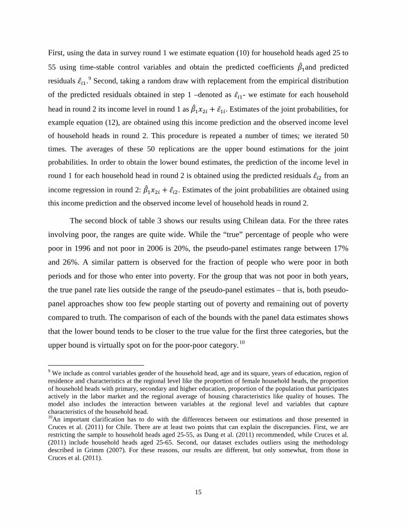
First, using the data in survey round 1 we estimate equation (10) for household heads aged 25 to
55 using time-stable control variables and obtain the predicted coefficients �̂�1and predicted
residuals 𝜀�̂�1.9 Second, taking a random draw with replacement from the empirical distribution
of the predicted residuals obtained in step 1 –denoted as 𝜀�̃�1- we estimate for each household
head in round 2 its income level in round 1 as �̂�1𝑥2𝑖 + 𝜀1̃𝑖. Estimates of the joint probabilities, for
example equation (12), are obtained using this income prediction and the observed income level
of household heads in round 2. This procedure is repeated a number of times; we iterated 50
times. The averages of these 50 replications are the upper bound estimations for the joint
probabilities. In order to obtain the lower bound estimates, the prediction of the income level in
round 1 for each household head in round 2 is obtained using the predicted residuals 𝜀�̂�2 from an
income regression in round 2: �̂�1𝑥2𝑖 + 𝜀�̂�2. Estimates of the joint probabilities are obtained using
this income prediction and the observed income level of household heads in round 2.
The second block of table 3 shows our results using Chilean data. For the three rates
involving poor, the ranges are quite wide. While the “true” percentage of people who were
poor in 1996 and not poor in 2006 is 20%, the pseudo-panel estimates range between 17%
and 26%. A similar pattern is observed for the fraction of people who were poor in both
periods and for those who enter into poverty. For the group that was not poor in both years,
the true panel rate lies outside the range of the pseudo-panel estimates – that is, both pseudo-
panel approaches show too few people starting out of poverty and remaining out of poverty
compared to truth. The comparison of each of the bounds with the panel data estimates shows
that the lower bound tends to be closer to the true value for the first three categories, but the
upper bound is virtually spot on for the poor-poor category.10
9 We include as control variables gender of the household head, age and its square, years of education, region of residence and characteristics at the regional level like the proportion of female household heads, the proportion of household heads with primary, secondary and higher education, proportion of the population that participates actively in the labor market and the regional average of housing characteristics like quality of houses. The model also includes the interaction between variables at the regional level and variables that capture characteristics of the household head. 10An important clarification has to do with the differences between our estimations and those presented in Cruces et al. (2011) for Chile. There are at least two points that can explain the discrepancies. First, we are restricting the sample to household heads aged 25-55, as Dang et al. (2011) recommended, while Cruces et al. (2011) include household heads aged 25-65. Second, our dataset excludes outliers using the methodology described in Grimm (2007). For these reasons, our results are different, but only somewhat, from those in Cruces et al. (2011).

16
The last pseudo-panel methodology is that proposed by Bourguignon et al. (2004) to
compute vulnerability-to-poverty mobility measures. The question these authors seek to
answer is: what is the probability of having an income below a poverty threshold conditional
on initial income and characteristics? We implemented this methodology using Chilean data
and following the procedure described in equations (6)-(9). At least three time periods are
required to be able to estimate the income dynamics coefficients in equation (8). Given that
restriction, we expand our Chilean dataset to include the 2001 round of the panel. However,
BGK point out that with three cross sections it is very likely that the parameter 𝜌𝑗 will be
very imprecisely estimated. In fact, for some of the cohorts –defined by birth and gender as
in the mean-based approach- we obtained values not acceptable for a correlation due to the
reduced sample size.11 In those cases, we impose the coefficient 𝜌𝑗 to be the same across a
number of cohorts using the nearest acceptable value. In order to compute the vulnerability-
to-poverty measure (equation (9)) we assumed stationarity of observable characteristics
𝑋�𝑖,𝑡+1𝑗 , earnings coefficients �̂�𝑡+1
𝑗 ,and variance of the innovation term 𝜎�𝜀𝑗,𝑡+12 .
The comparison of the true panel and pseudo-panel estimates is shown in the last
block of table 3. While the actual frequency of people falling into or remaining in poverty in
2006 is 14.47%, the pseudo-panel method predicts a value almost twice as high as the panel
figure (24.64%). Even though the difference is very large, it is important to consider the
restriction imposed by the small number of cross-section surveys.
To conclude, for the most part, we do not obtain good estimations using pseudo panels
to answer the specific questions each author proposed (where good is close to the true panel
result). The only question for which the pseudo-panel method approximates the true panel
result is the estimate of the unconditional 𝛽 coefficient.
4.2 Pseudo panels’ performance answering general questions
11 OLS estimation of equation (8) does not automatically satisfy the condition that the estimated coefficient must be between zero and one. BGK establish that this might be remedied by imposing some restriction on the parameter ρj across cohorts j.

17
We now compute a broader set of income mobility measures and focus on how close or far
pseudo-panel methods come in approximating the full set of macro-mobility measures,
micro-mobility regression coefficients, and poverty transition rates presented in table 1.
Our results are shown in table 4. As shown in the first block of the table, for the
macro-mobility measures the pseudo-panel estimates are quite far off and tend to
underestimate substantially the true degree of income mobility. They show too much time
dependence, and therefore too little mobility-as-time-independence, with the exception of the
upper bound estimation using the DLLM methodology that is closer to the true value; about
the right amount of positional movement, with the exception of the BGK estimate that shows
too little mobility; too little share movement, although the upper bound is closer to the true
value; too little non-directional income movement– that is, incomes change much more in the
true panel than is seen in the pseudo panels- and again the upper bound is closer to the true
value; about the right amount of directional income movement, especially for the mean-based
approach and the BGK methodology, but this is true only on average, the pseudo panels
show too little of upward and downward movements; the mean-based approach and the upper
bound show too much equalization of longer-term income relative to initial, while the lower
bound and the BGK pseudo panel show too little.
To sum up, none of the pseudo-panel approaches gives good approximations for all of
the macro-mobility concepts. Furthermore, the lower and upper bounds do not contain the
true value for some of the measures, and we cannot conclude that one of the bounds provides
better estimates than the other.
Our findings on the micro-mobility regression coefficients are shown in the second
block of table 4. For the true panel, we find substantial convergence, both in logs (“weak”)
and in pesos (“strong”), both unconditionally and conditionally. The mean-based approach
also predicts a pattern of income convergence both in logs and in pesos, but this approach
underestimates the degree of strong income convergence and overestimates the degree of
weak income convergence. The DLLM lower and upper bounds contain the regression
coefficients estimated using true panel data. However, the width of these bounds is so wide
as to be useless. For instance, the lower bound predicts a pattern of income divergence under
the strong convergence hypothesis, while the upper bound predicts negative coefficients that

18
are larger (in absolute value) than panel data estimations. Finally, the BGK pseudo panel
predicts coefficients with the right sign but they are very far from the true values in a
systematic direction: the BGK method estimates considerably less convergence than the true
panel does. As was mentioned before, we start working with the same sample of household
heads from the panel and then apply the pseudo-panel calculations. The lower number of
observations in DLLM micro-regression coefficients compared with the panel is explained
by the age restriction of the method (it predicts future incomes for household heads between
25 and 55 years old) and the missing values in the explanatory variables used in the income
regressions, while the lower number of observations in BGK micro-regression coefficients
compared with the panel is explained by the birth-cohort construction (people belonging to
some cohort are between 20 and 65 years of age).
In the last block of table 4 we show our poverty dynamics results. The conclusion is
that pseudo-panel methods fail to predict accurately the percentage that crossed the poverty
line. Two of the pseudo-panel methods (the DLLM method and BGK method) substantially
understate the probability of those who were poor in period 1 escaping from poverty by
period 2, and all of the pseudo-panel methods understate the probability of falling into
poverty in period 2 conditional on not being in poverty in period 1. In short, the pseudo-panel
methods reveal way too few poverty transitions compared to the true panel.
In sum, using Chilean data for the period 1996-2006 we conclude that not only do
pseudo panels fail to predict the mobility measures they were intended to estimate (with the
only exception of the mean-based approach estimating beta unconditionally), but also they
perform poorly in predicting a broader set of income mobility measures.
5. Joint probability of poverty status versus poverty dynamics
The pseudo-panel method proposed by DLLM calculates the joint probability of poverty
status in t1 and t2. Even though those estimates provide valuable information about
movements into and out of poverty, they do not represent poverty dynamics, which by
definition is a conditional concept. For instance, the probability of being non-poor in t=2 for
those who were poor in t=1 is a poverty dynamic measure, and likewise for the other
conditional transition rates. In the bottom block of table 4 we reported our poverty dynamics

19
estimates using the DLLM pseudo-panel method applied to our data for Chile. As we
mentioned before, the results are not encouraging. The panel data estimate does not lie
between the lower and upper bound estimates, and none of the bounds gives a good
prediction of the true poverty transition rates.
In this section we reproduce the results obtained by Cruces et al. (2011) for the case of
Chile (top block of table 5) and reformulate them as conditional probabilities (bottom block
of table 5).12 The main objective is to compare how close true panel poverty transition rates
are to the pseudo-panel figures. The findings indicate that “true” poverty transition rates lie
between the lower and upper bounds predicted by the DLLM method. However, the width of
the bounds in the conditional formulation is much greater than in the original calculations as
joint probabilities. For instance, in the top block of the table, we see that the probability of
being poor in 1996 and not being poor in 2006 is predicted to range between 11% and 21%,
i.e., the width of the bounds is 10 percentage points. On the other hand, in the bottom block
of the table, we see that the probability of not being poor in 2006, conditional on being poor
in 1996, ranges between 67.5% and 89.9%, i.e., the width of the bounds is 22 percentage
points. Thus, the width of the bounds when the probability is computed as a poverty dynamic
measure is twice as large as in the joint probability formulation. In this sense, the DLLM
pseudo panel provides only limited information about poverty transition rates.
6. Conclusions
The general question this paper intended to answer was: are pseudo panels a suitable
substitute for true panels for estimating income mobility? In order to obtain evidence and
give an answer to this question we constructed pseudo panels using Chilean panel data and
treating each round of the panel as if it were an independent cross-section survey. We
considered three different pseudo-panel methods available in the literature. First, the mean-
based approach that identifies cohorts, and follows cohort means over time. Second, the
method developed by Bourguignon, Goh and Kim that was designed to estimate
vulnerability-to-poverty measures in the absence of panel data. Third, the pseudo-panel 12 As we mentioned in section 4, results in Cruces et al. (2011) differ from our estimates. These differences are explained by (i) the restriction of the sample to household heads aged 25-55, while Cruces et al. (2011) use a wider age group (25-65); (ii) our dataset excludes outliers as in Grimm (2007).

20
method of Dang, Lanjouw, Luoto and McKenzie that predicts a lower and upper bound for
the joint probabilities of poverty status in t=1 and t=2. These techniques differ from one
another in terms of data demands, assumptions about structural parameters and functional
forms, and in the mobility question they attempt to answer.
In order to organize the analysis, we proceeded in two steps. First, we evaluated how
the pseudo-panel methods perform in answering the specific income mobility question they
were devised to answer. Second, we computed a broader set of income mobility measures
and focused on how close or far pseudo-panel methods come in approximating macro-
mobility measures, micro-mobility regression coefficients, and poverty transition rates.
According to the empirical evidence we have obtained using Chilean panel data for
the period 1996-2006, our conclusion is that pseudo-panel methodologies do not perform
well in this task. Our results indicate that pseudo panels fail in two respects when trying to
predict the income mobility pattern observed in Chile. First, they do not give good results for
the mobility concept each pseudo-panel method sought to measure. The only exception was
the unconditional estimation of the mean-based approach. Second, they also perform poorly
in predicting a broader set of income mobility measures.
Finally, we extended the analysis including a reformulation of the calculations
proposed by Dang, Lanjouw, Luoto and McKenzie. These authors calculated the joint
probabilities of poverty status in t1 and t2. Using the results presented by Cruces et al. (2011)
for the case of Chile, we re-expressed them as poverty dynamics measures, i.e., conditional
probabilities. The results were not encouraging. Even though the “true” poverty transition
rates lie between the lower and upper bounds predicted by the method, the width of the
bounds in the conditional formulation is much greater than in the original calculations as
joint probabilities. In this sense, the DLLM pseudo panel provides only limited information
about poverty transition rates.

21
7. References
Antman, F. and McKenzie, D. (2007): “Earnings Mobility and Measurement Error: A Pseudo-Panel Approach”. Economic Development and Cultural Change, vol. 56(1), pp. 125-161.
Bourguignon, F. Goh, Ch. and Kim, D. (2004): “Estimating Individual Vulnerability to Poverty with Pseudo-Panel Data”. World Bank Policy Research Working Paper No. 3375.
Calónico, S. (2006): “Pseudo-Panel Analysis of Earnings Dynamics and Mobility in Latin America”. Mimeo, Inter-American Development Bank.
Castro, R. (2011): “Getting Ahead, Falling Behind and Standing Still. Income Mobility in Chile”. Estudios de Economía, Vol. 38, N 1, pp. 243-258.
Collado, D. (1997): “Estimating Dynamic Models from Time Series of Independent Cross Sections”. Journal of Econometrics, 82, pp. 37–62.
Cruces, G., Lanjouw, P., Lucchetti, L., Perova, E., Vakis, R. and Viollaz, M. (2011): “Intra-generational Mobility and Repeated Cross-Sections. A Three-country Validation Exercise”. World Bank Policy Research Working Paper No. 5916.
Cuesta, J., Ñopo, H. and Pizzolitto, G. (2011): “Using Pseudo-Panels to Measure Income Mobility in Latin America”. The Review of Income and Wealth, serie 57(2).
Dang, H., Lanjouw, P., Luoto, J. and McKenzie, D. (2011): “Using Repeated Cross-Sections to Explore Movements into and out of Poverty”. World Bank Policy Research Working Paper No. 5550.
Deaton, A.(1985): “Panel Data from Time Series of Cross-Sections”. Journal of Econometrics 30, pp. 109-216.
Ferreira, F., Messina, J., Rigolini, J., López-Calva, L.F., Lugo, M.A. and Vakis, R. (2013): “Economic Mobility and the Rise of the Latin American Middle Class”. Washington, DC: World Bank.
Fields, G., Duval Hernandez, R., Freije Rodriguez, S. and Sanchez Puerta, M.L. (2007): “Intergenerational Income Mobility in Latin America”. Journal of LACEA.Latin American and Caribbean Economic Association.
Grimm, M. (2007): “Removing the Anonymity Axiom in Assessing Pro-Poor Growth”, Journal of Economic Inequality, 5(2), pp 179–197.
McKenzie, D. (2001): “Estimation of AR(1) models with unequally spaced pseudo-panels”. Econometric Journal, Royal Economic Society, vol. 4(1).
McKenzie, D. (2004): “Asymptotic Theory for Heterogeneous Dynamic Pseudo-Panels”. Journal of Econometrics, Elsevier, vol. 120(2), pp. 235-262.
Moffitt, R. (1993): “Identification and Estimation of Dynamic Models with a Time Series of Repeated Cross-Sections”. Journal of Econometrics, vol. 59, pp. 99–124.
Navarro, A. (2006): “Estimating Income Mobility in Argentina with Pseudo-Panel Data”. Mimeo, Universidad de San Andrés.

22
SEDLAC (2012). Socio-Economic database for Latin America and the Caribbean, CEDLAS and The World Bank. http://sedlac.econo.unlp.edu.ar/eng/index.php.
Verbeek, M. and Vella, F. (2005): “Estimating Dynamic Models from Repeated Cross-Sections”. Mimeo, K.U. Leuven Center for Economic Studies.
WDI (2012). World Development Indicators, The World Bank. http://data.worldbank.org/data-catalog/world-development-indicators

23
Tables
Table 1: Income mobility measures using panel data Chile 1996-2006
Source: Own elaboration based on CASEN 1996-2006 and SEDLAC (CEDLAS and World Bank). Notes: Shares are computed as the participation of per capita household income in average national income in each of the years. Conditional regressions include age of the household head and its square, gender, years of education and its square, and region of residence. In the mobility as an equalizer of longer-term incomes a is the vector of average incomes, y1 is the vector of first-year incomes, and I(.) is a Lorenz-consistent inequality measure. We use the Gini coefficient.
Macromobility concept
Time independence
[1 - Pearson's correlation coefficient] 0.810
Positional movement
Mean absolute value of decile change 2.172
Share movements
Mean absolute value of share change 0.628
Non-directional income movement
Mean absolute value of income change 58,548
Directional income movement
Mean income change 17,586 std. desv. 171,935
Percentage of upward movers 64.35 Percentage of downward movers 35.65 Average income gains of the upward movers 59,158 Average income losses of the downward movers -57,447
Mobility as an equalizer of longer-term incomes
ε ≡1-(I(a)/I(y 1 )) 0.168
Micromobility regression
Change in pesos – unconditional regression coefficient -0.628 Standard error [0.057]*** R2 0.10 N 2552
Change in pesos – conditional regression coefficient -0.761 Standard error [0.048]*** R2 0.12 N 2465
Change in log pesos – unconditional regression coefficient -0.579 Standard error [0.030]*** R2 0.40 N 2527
Change in log pesos – conditional regression coefficient -0.709 Standard error [0.034]*** R2 0.48 N 2441
Poverty dynamics and crossing the poverty line measures
Probability of not being poor in t=2, conditional on being poor in t=1 70.83 Probability of being poor in t=2, conditional on not being poor in t=1 5.94

24
Table 2: Definition and size of birth-gender cohorts Chile 1996-2006
Source: Own elaboration based on CASEN 1996-2006 and SEDLAC (CEDLAS and World Bank).
1996 2006 1996 20061931-1932 2 2 4 101 116 2171933-1934 2 2 4 81 91 1721935-1936 2 2 4 79 94 1731937-1938 2 2 4 109 114 2231939-1940 2 2 4 120 129 2491941-1942 2 2 4 121 134 2551943-1944 2 2 4 111 125 2361945-1946 2 2 4 120 137 2571947-1948 2 2 4 127 134 2611949-1950 2 2 4 112 125 2371951-1952 2 2 4 106 135 2411953-1954 2 2 4 117 142 2591955-1956 2 2 4 143 165 3081957-1958 2 2 4 142 168 3101959-1960 2 2 4 152 169 3211961-1962 2 2 4 122 153 2751963-1964 2 2 4 124 160 2841965-1966 2 2 4 97 125 2221967-1968 2 2 4 70 96 1661969-1970 2 2 4 62 98 1601971-1972 2 2 4 41 80 1211973-1974 2 2 4 27 83 1101975-1976 2 2 4 6 49 55Total 46 46 92 2,290 2,822 5,112
Year-birth cohort
Time period Total synthetic individuals
Time period Total household observations

25
Table 3: Pseudo-panel performance answering specific income mobility questions Chile 1996-2006
Source: Own elaboration based on CASEN 1996-2006 and SEDLAC (CEDLAS and World Bank).
Mean-based approachPseudo panel
Panel data
β - unconditional 0.438 0.421 Standard error [0.067]*** [0.030]*** R2 0.54 0.26
β - conditional 0.150 0.291 Standard error [0.129] [0.034]*** R2 0.69 0.36
Dispersion-based approachDLLM methodology
PanelLower bound Upper bound data
Poor - Non Poor 17.41 25.60 20.22Non Poor - Poor 2.70 9.18 4.97Non Poor - Non Poor 62.92 56.31 64.93Poor - Poor 16.96 8.91 9.88
BGK methodology
Pseudo panel Panel data
Predicted rate of poverty in 2006 24.64
Rate of poverty in 2006 14.47
Pseudo - panel

26
Table 4: Pseudo-panel performance answering other income mobility questions Chile 1996-2006
Lower bound Upper bound
Macromobility concept
Time independence
[1 - Pearson's correlation coefficient] 0.810 0.365 0.151 0.766 0.094
Positional movement Mean absolute value of decile change 2.172 1.609 1.061 2.432 0.743
Share movements
Mean absolute value of share change 0.628 0.219 0.278 0.575 0.269
Non-directional income movement
Mean absolute value of income change 58,548 23,508 34,846 60,994 30,808
Directional income movement
Mean income change 17,586 18,905 30,414 37,075 22,709 std. desv. 171,935 25,815 42,490 69,845 36,360
Percentage of upward movers 64.35 89.13 85.97 79.69 88.39 Percentage of downward movers 35.65 10.87 14.03 20.31 11.61 Average income gains of the upward movers 59,158 23,792 37,957 61,534 30,273 Average income losses of the downward movers -57,447 -21,176 -15,791 -58,876 -34,876
Mobility as an equalizer of longer-term incomes
ε ≡1-(I(a)/I(y1)) 0.168 0.202 0.091 0.345 0.123
DLLM methodDispersion based approach
Pseudo-panel
Mean based approach BGK
method
Panel data

27
Table 4: Pseudo-panel performance answering other income mobility questions – cont. Chile 1996-2006
Source: Own elaboration based on CASEN 1996-2006 and SEDLAC (CEDLAS and World Bank). Notes: In the mobility as an equalizer of longer-term incomes a is the vector of average incomes, y1 is the vector of first-year incomes, and I(.) is a Lorenz-consistent inequality measure. We use the Gini coefficient. The lower number of observations in DLLM micro-regression coefficients compared with the panel is explained by the age restriction of the method (it predicts future incomes for household heads between 25 and 55 years old).The lower number of observations in BGK micro-regression coefficients compared with the panel is explained by the birth-cohort construction (people belonging to some cohort are between 20 and 65 years of age).
Lower bound Upper boundMicromobility regression
Change in pesos – unconditional regression coefficient -0.628 -0.409 0.271 -0.751 -0.155 Standard error [0.057]*** [0.158]** [0.052]*** [0.077]*** [0.035]*** R2 0.10 0.23 0.11 0.35 0.13 N 2552 46 1525 1525 2124
Change in pesos – conditional regression coefficient -0.761 -0.627 0.269 -1.043 -0.290 Standard error [0.048]*** [0.202]*** [0.056]*** [0.050]*** [0.024]*** R2 0.12 0.41 0.18 0.57 0.66 N 2465 46 1520 1520 2124
Change in log pesos – unconditional regression coefficient -0.579 -0.613 -0.111 -0.744 -0.224 Standard error [0.030]*** [0.052]*** [0.015]*** [0.037]*** [0.012]*** R2 0.40 0.73 0.05 0.58 0.37 N 2527 46 1525 1525 2124
Change in log pesos – conditional regression coefficient -0.709 -0.891 -0.063 -0.995 -0.385 Standard error [0.034]*** [0.116]*** [0.018]*** [0.027]*** [0.010]*** R2 0.48 0.84 0.18 0.74 0.82 N 2441 46 1520 1520 2124
Poverty dynamics and crossing the poverty line measures
Probability of not being poor in t=2, conditional on being poor in t=1 70.83 75.00 37.51 66.80 56.03 Probability of being poor in t=2, conditional on not being poor in t=1 5.94 0.00 1.76 1.08 0.09
Pseudo-panel
Mean based approach
Dispersion based approachDLLM method BGK
method
Panel data

28
Table 5: DLLM method – Joint and conditional probabilities Chile 1996-2006
Source: Own elaboration based on Cruces et al. (2011).
Joint probabilities
Lower bound Upper boundProbability of being poor in t=1 and t=2 4.64 5.35 2.61 -2.74Probability of being poor in t=1 and not being poor in t=2 19.59 11.09 21.50 10.41Probability of not being poor in t=1 and t=2 72.82 81.31 70.90 -10.41Probability of not being poor in t=1 and being poor in t=2 2.96 2.25 4.98 2.73
Conditional probabilities
Lower bound Upper boundProbability of being poor in t=2, conditional on being poor in t=1 19.15 32.54 10.15 -22.39Probability of not being poor in t=2, conditional on being poor in t=1 80.85 67.46 89.85 22.39Probability of being poor in t=2, conditional on not being poor in t=1 3.91 2.69 6.77 4.08Probability of not being poor in t=2, conditional on not being poor in t=1 96.09 97.31 93.23 -4.08
Panel data DLLM method
Width of the bounds
Width of the bounds
Panel data DLLM method


